$\cal K$  UCP $\cal K$  UCP                                                                                                KUCP-0172 hep-th/0011091  

D-branes on a Noncompact Singular Calabi-Yau Manifold

 

Katsuyuki Sugiyama

Department of Fundamental Sciences, Faculty of Integrated Human Studies, Kyoto University, Yoshida-Nihonmatsu-cho, Sakyo-ku, Kyoto 606-8501, Japan.

E-mail: sugiyama@phys.h.kyoto-u.ac.jp

Satoshi Yamaguchi

Graduate School of Human and Environmental Studies, Kyoto University, Yoshida-Nihonmatsu-cho, Sakyo-ku, Kyoto 606-8501, Japan.

E-mail: yamaguch@phys.h.kyoto-u.ac.jp

Abstract:   We investigate D-branes on a noncompact singular Calabi-Yau manifold by using the boundary CFT description, and calculate the open string Witten indices between the boundary states. The B-type D-branes turn out to be characterized by the properties of a compact positively curved manifold. We give geometric interpretations to these boundary states in terms of coherent sheaves of the manifold.

1 Introduction

D-branes are the key objects by which we can study the nature of various string theories. The Cardy’s boundary CFT method [1] is a very powerful tool to investigate the D-branes in curved spaces.

Recently, there has been great progress[2, 3] in the study of properties of charges, boundary states[4, 1] based on Gepner models[5, 6]. For a large class of Calabi-Yau manifolds, associated boundary states have been constructed and susy cycles have been investigated based on these states in CFTs[7, 8, 9, 10, 11], [2, 3, 12, 13, 14, 15, 16, 17, 18]. These references consider D-branes as the “rational boundary states” , that is, the Cardy states realized as some linear combinations of tensor products of Ishibashi states of each minimal model. There appear many consistency checks about their charges, the intersection form of the homology cycles. However these analyses are restricted to compact Calabi-Yau cases.

In [19], Giveon et al. proposed that a string theory on a noncompact singular Calabi-Yau manifold $X$ represented by a hypersurface $F(z_{1},\dots,z_{n+1})=0\text{ in }{\mathbb{C}}^{n+1}$ can be described by a CFT as ${\mathbb{R}}_{\phi}\times S^{1}\times LG(W=F)$. Here ${\mathbb{R}}_{\phi}$ is a linear dilaton and $LG(W=F)$ is the two dimensional ${\cal N}=2$ Landau-Ginzburg theory with the superpotential $F$.

Also, in [20, 21, 22, 23, 24], the modular invariant partition functions can be constructed in the cases that $LG(W=F)$’s are minimal models or direct products of minimal models, and it is shown that associated string theories on these singular spaces can exist consistently. They are extensions of Gepner models from compact manifolds to noncompact varieties with singularities.

The aim of this paper is to develop a method to construct boundary states of noncompact singular Calabi-Yau manifolds and to investigate their properties in order to understand structures of moduli spaces in the open string channel. In this paper, we explore the “rational” D-branes on a noncompact singular Calabi-Yau manifold by applying the Cardy’s method to the Gepner-like description of the noncompact singular Calabi-Yau manifold.

As a result, the open string Witten index turns out to be factorized into $\theta_{1}(\tau)(=0)$ factor and a nontrivial one, in the same way as the closed string Witten index[22] does. We investigate the nontrivial factor in the open string Witten index and show that they coincide with some pairings of bundles in the manifold $X/{\mathbb{C}}^{\times}$.

To confirm the validity of this claim, we calculate the relative Euler characteristics of the bundles in $X/{\mathbb{C}}^{\times}$ by applying geometrical methods to a special case, where $X/{\mathbb{C}}^{\times}$ is written as a Fermat type hypersurface $z_{1}^{N}+\dots+z_{r}^{N}=0$ in ${\mathbb{C}}P^{r-1}$. We compare it with the result in the CFT calculations.

The paper is organized as follows. In section 2, we review the Gepner-like description of noncompact singular Calabi-Yau manifolds and fix our convention. In section 3, we construct the boundary states of the noncompact manifold in the Gepner-like description and study intersection number between these states. This intersection pairing is understood as a combination of characteristic classes with a pair of boundary bundles and we compare the result in the CFT with the geometrical ones. We give geometrical interpretations to the boundary states in terms of coherent sheaves in section 4. Charges of D-branes wrapped on the susy cycles are realized as characteristic classes of the sheaves. Section 5 is devoted to conclusions and discussions. In appendix A, we summarize several useful properties of theta functions. Periods near the orbifold point are collected in appendix B. Also formulas of periods in the large volume region are shown concretely in appendix C.

2 The closed string theory on a noncompact singular Calabi-Yau manifold

In this section, we summarize the Gepner-like description of the closed string theory on a noncompact singular Calabi-Yau $n$-fold $X$. We mainly use the same conventions as in the paper[22].

We assume that the $X$ is realized as a zero locus $F(z_{1},\dots,z_{n+1})=0$ in ${\mathbb{C}}^{n+1}$, where $F(z)$ is a quasi-homogeneous polynomial, i.e. it satisfies the relation

$$F(\lambda^{r_{1}}z_{1},\dots,\lambda^{r_{n+1}}z_{n+1})=\lambda F(z_{1},\dots,z_{n+1})\qquad\mbox{for}\,\,\,{}^{\exists}r_{j}\in{\mathbb{R}},{}^{\forall}\lambda\in{\mathbb{C}}^{\times}\,.$$

It is proposed in [19] that the string theory on $X$ is described by a model

$${\mathbb{R}}_{\phi}\times S^{1}\times LG(W=F),$$

where ${\mathbb{R}}_{\phi}$ is a real line with a linear dilaton background and $LG(W=F)$ is a scale invariant theory realized in the IR limit of the Landau-Ginzburg theory with the superpotential $F$. In this paper we consider the case where $LG(W=F)$ is described as a direct product of A-type minimal models, namely, the polynomial $F$ is written as a linear combination of constituent minimal models

$$F(z_{1},\dots,z_{n+1})=z_{1}^{N_{1}}+\dots+z_{r}^{N_{r}}+z_{r+1}^{2}+\dots+z_{n+1}^{2}.$$ (2.1)

Here the Landau-Ginzburg theory is composed of $r$ minimal models and the level of the $j$-th minimal model is $N_{j}-2$.

The remaining parts ${\mathbb{R}}_{\phi}\times S^{1}$ also have worldsheet ${\cal N}=2$ superconformal symmetry. We denote the bosonic coordinates of ${\mathbb{R}}_{\phi}$ and $S^{1}$ by $\phi$ and $Y$, respectively, and the fermionic counterparts of ${\mathbb{R}}_{\phi}$ and $S^{1}$ by the free fermions $\psi^{\pm}$. Then the ${\cal N}=2$ superconformal currents are expressed as

$$T=-\frac{1}{2}(\partial Y)^{2}-\frac{1}{2}(\partial\phi)^{2}-\frac{Q}{2}\partial^{2}\phi-\frac{1}{2}(\psi^{+}\partial\psi^{-}-\partial\psi^{+}\psi^{-}),$$

$$G^{\pm}=-\frac{1}{\sqrt{2}}\psi^{\pm}(i\partial Y\pm\partial\phi)\mp\frac{Q}{\sqrt{2}}\partial\psi^{\pm},$$

$$J=\psi^{+}\psi^{-}-Qi\partial Y.$$ (2.2)

The Liouville field $\phi$ has a background charge $Q$ and the associated central charge of this algebra is given as $\hat{c}\;(:=c/3)=1+Q^{2}$. Since we are considering the string theory on a Calabi-Yau $n$-fold, the central charge should satisfy the consistency condition $\hat{c}=n$. When we take into account of the background charge $Q$ of ${\mathbb{R}}_{\phi}$, the condition on the central charge is represented as

$$1+Q^{2}+\sum_{j=1}^{r}\frac{N_{j}-2}{N_{j}}=n.$$

It means that the background charge $Q$ is determined from the parameters of the minimal models $r$, $N_{j}$ through a relation

$$Q^{2}=n-1-r+\sum_{j=1}^{r}\frac{2}{N_{j}}.$$

For simplicity, we concentrate on the case that $n-1-r\equiv 0\mod 2$ in this paper. Then $KQ^{2}$ is an even integer with $K={\rm lcm}(N_{j})$ and we can define an integer $J$ as

$$J:=\frac{KQ^{2}}{2}\in{{\mathbb{Z}}}.$$

Next, let us construct the modular invariant partition function of this model and determine the spectrum. As a consistency condition, we have to pick up only the states with integral $U(1)$ charges since we want a Calabi-Yau CFT. First the linear dilaton $\phi$ does not have any $U(1)$ charge and we can independently consider the partition function $Z_{L}$ of $\phi$ [20]

$$Z_{L}(\tau,\bar{\tau})=\frac{1}{\sqrt{\tau_{2}}|\eta(\tau)|^{2}},$$

where $\eta(\tau)$ is the Dedekind eta function.

The other parts, $Y,\psi^{\pm}$ and fields in the minimal models carry $U(1)$ charges, and we must apply the GSO projection to them. Let us consider first the case of $Y$. If we consider the Verma module with primary field $e^{ipY}$ for a real number $p$, the character of this Verma module is $q^{p^{2}/2}/\eta(\tau)$, where $q=\exp(2\pi i\tau)$. One can see the $U(1)$ charge of the states in this Verma module is $pQ$. We should take the case that $KpQ$ is an integer, since the $U(1)$ charge of the other part is $(\text{integer})/K$ and the total $U(1)$ charge should be an integer. If we write $KpQ=2KJu+m_{0}$ with two integers $u,m_{0}$ and sum up the character for all $u\in{\mathbb{Z}}$, then we obtain the relation

$$\sum_{u\in{\mathbb{Z}}}\frac{q^{\frac{1}{2}p^{2}}}{\eta(\tau)}=\frac{\Theta_{m_{0},KJ}(\tau)}{\eta(\tau)}.$$

Note that the $U(1)$ charges of the states included in these Verma module are $m_{0}/K\mod 2J$.

Next we shall consider fermionic parts. The Verma modules of two fermions $\psi^{\pm}$ are characterized by an integer $s_{0}=0,1,2,3$. The states with $s_{0}=0,2$ belong to the NS sector, and ones with $s_{0}=1,3$ are states in the R sector. The characters of these Verma modules are expressed by using theta functions $\Theta_{s_{0},2}(\tau)/\eta(\tau)$.

Last we study the Verma modules of a minimal model. An arbitrary Verma module in this model is labelled by three integers $(\ell,m,s)$. They take their values in the following ranges

$$\ell=0,1,\dots,N-2,$$

$$m=0,1,\dots,2N-1,$$

$$s=0,1,2,3,$$

$$\ell+m+s\equiv 0\mod 2.$$ (2.3)

The states with $s_{0}=0,2$ belong to the NS sector, and ones with $s_{0}=1,3$ are states in the R-sector. From now on, we denote the character of this Verma module as $\chi_{m}^{\ell,s}(\tau)$

In order to consider the whole Verma module of a set of minimal models, we introduce the following vector notations

$$\vec{\ell}=(\ell_{1},\dots,\ell_{r}),\quad\vec{m}=(m_{0},m_{1},\dots,m_{r}),\quad\vec{s}=(s_{0},s_{1},\dots,s_{r}),\quad{\sf a}=(\vec{\ell},\vec{m},\vec{s})$$

where $(\ell_{j},m_{j},s_{j}),\ j=1,\dots,r$ is a set of indices of the Verma module in the $j$-th minimal model and $m_{0}$ and $s_{0}$ were defined above. By collecting contributions of constituent minimal models, we can write down the character of the Verma module for $(\vec{\ell},\vec{m},\vec{s})$ as

$$f_{{\sf a}}(\tau)=\frac{\Theta_{s_{0},2}(\tau)}{\eta(\tau)}\frac{\Theta_{m_{0},KJ}(\tau)}{\eta(\tau)}\chi_{m_{1}}^{\ell_{1},s_{1}}(\tau)\dots\chi_{m_{r}}^{\ell_{r},s_{r}}(\tau).$$

As a consistency condition, we must impose a modular invariance on the total partition function, and moreover we may use only the states with integral U(1) charges since we want a Calabi-Yau CFT. For this purpose, we will write down the transformation laws of the characters $f_{\sf a}$ under the modular transformations $\tau\rightarrow\tau+1$ and $\tau\rightarrow-1/\tau$

$$f_{\sf a}(\tau+1)=\,{\bf e}\!\left[-\frac{1}{2}(\vec{m}\bullet\vec{m}+\vec{s}\bullet\vec{s})\right]f_{\sf a}(\tau),$$

$$f_{\sf a}(-1/\tau)=\sum_{{\sf a}^{\prime}}^{\rm even}S_{{\sf a}{\sf a}^{\prime}}f_{{\sf a}^{\prime}}(\tau),$$

$$S_{{\sf a}{\sf a}^{\prime}}:=A_{\vec{\ell}\vec{\ell}^{\prime}}\left(\prod_{j}\frac{1}{\sqrt{8N_{j}}}\right)\frac{1}{\sqrt{8KJ}}\,{\bf e}\!\left[\vec{m}\bullet\vec{m}^{\prime}+\vec{s}\bullet\vec{s}^{\prime}\right],$$

$$A_{\vec{\ell}\vec{\ell}^{\prime}}:=\prod_{j=1}^{r}A_{\ell_{j}\ell_{j}^{\prime}}=\prod_{j=1}^{r}\sqrt{\frac{2}{N_{j}}}\sin\pi\frac{(\ell_{j}+1)(\ell_{j}^{\prime}+1)}{N_{j}},$$

$$\vec{m}\bullet\vec{m}^{\prime}:=-\frac{m_{0}m_{0}^{\prime}}{2KJ}+\sum_{j=1}^{r}\frac{m_{j}m_{j}^{\prime}}{2N_{j}},$$

$$\vec{s}\bullet\vec{s}^{\prime}:=-\frac{s_{0}s_{0}^{\prime}}{4}-\sum_{j=1}^{r}\frac{s_{j}s_{j}^{\prime}}{4}.$$

To make a modular invariant partition function with these states, we further introduce a special vector ${\vec{\beta}}$ in the same type of $\vec{m}$

$${\vec{\beta}}=(-2J,2,\dots,2).$$

Then, the charge integrality condition can be expressed as the following “beta constraint”

$$-\frac{m_{0}}{K}+\sum_{j=1}^{r}\frac{m_{j}}{N_{j}}={\vec{\beta}}\bullet\vec{m}\in{\mathbb{Z}}\,.$$ (2.4)

With these notations, we write down the NS-sector partition function as a combination of characters

$$\operatorname*{{\rm Tr}}_{\rm NSNS}\left[q^{L_{0}-\frac{\hat{c}}{8}}\bar{q}^{\bar{L}_{0}-\frac{\hat{c}}{8}}\right]=\frac{1}{\sqrt{\tau_{2}}|\eta(\tau)|^{2}}\sum_{b\in{\mathbb{Z}}_{K}}\sum_{\begin{subarray}{c}\vec{\ell},\vec{m},\\ \vec{s},\vec{\bar{s}}=0,2,\\ \ell_{j}+m_{j}\equiv 0\mod 2,\\ {\vec{\beta}}\bullet\vec{m}\in{\mathbb{Z}}\end{subarray}}f_{(\vec{\ell},\vec{m},\vec{s})}(\tau)\bar{f}_{(\vec{\ell},\vec{m}+b{\vec{\beta}},\vec{\bar{s}})}(\bar{\tau}).$$ (2.5)

Similarly the RR-sector counterpart can also be calculated as

$$\operatorname*{{\rm Tr}}_{\rm RR}\left[(-1)^{F}q^{L_{0}-\frac{\hat{c}}{8}}\bar{q}^{\bar{L}_{0}-\frac{\hat{c}}{8}}\right]$$

$$\qquad=\frac{1}{\sqrt{\tau_{2}}|\eta(\tau)|^{2}}\sum_{b\in{\mathbb{Z}}_{K}}\sum_{\begin{subarray}{c}\vec{\ell},\vec{m},\\ \vec{s},\vec{\bar{s}}=1,3,\\ \ell_{j}+m_{j}\equiv 1\mod 2,\\ {\vec{\beta}}\bullet\vec{m}\in{\mathbb{Z}}\end{subarray}}f_{(\vec{\ell},\vec{m},\vec{s})}(\tau)\bar{f}_{(\vec{\ell},\vec{m}+b{\vec{\beta}},\vec{\bar{s}})}(\bar{\tau})(-1)^{\sum_{j}(s_{j}-\bar{s}_{j})/2+b}.$$

(2.6)

It is nothing but a Witten index of the model and geometrical properties of the target manifolds are encoded in this formula.

We can check that these partition functions actually satisfy the right modular properties and construct consistent string theories propagating in singular target manifolds. The picture in this section is based on the closed strings on the singular manifolds. However D-branes couple with strings only through open strings and it is important to develop a method to describe open strings in these models. The open strings can end on susy cycles of the target manifolds and encode information on homology cycles of the manifolds. In the context of CFT, we are able to analyze properties of these boundaries of the open strings based on the boundary states. In the next section, we will construct boundary states associated with these singular manifolds and investigate their properties.

3 Boundary states and the intersection form

3.1 The open string in the ${\cal N}=2$ Liouville theory

Here we consider D-branes in our model and analyze the properties of the associated open strings. Generally it is known that two types (A-type and B-type) of boundary conditions are possible for ${\cal N}=2$ superconformal currents. These boundary conditions in the open string channel are defined on the worldsheet boundary $z=\bar{z}$;

• A-type boundary condition

  $$T=\bar{T},\ G^{\pm}=\varepsilon\bar{G}^{\mp},\ J=-\bar{J}.$$

• B-type boundary condition

  $$T=\bar{T},\ G^{\pm}=\varepsilon\bar{G}^{\pm},\ J=+\bar{J}.$$

Here, $\varepsilon=1$ in R-sector with $z>0$ and NS-sector, $\varepsilon=-1$ in R-sector with $z<0$ . First we consider the boundary conditions in the ${\cal N}=2$ Liouville sector. Using ${\cal N}=2$ superconformal currents represented by free fields (2.2), we express the boundary conditions for free fields $\phi$, $Y$ and $\psi^{\pm}$;

• A-type

  $$\partial\phi=\bar{\partial}\phi\text{ (Neumann) },\ \partial Y=-\bar{\partial}Y\text{ (Dirichlet) },\ \psi^{\pm}=\varepsilon\bar{\psi}^{\mp}.$$

• B-type

  $$\partial\phi=\bar{\partial}\phi\text{ (Neumann) },\ \partial Y=+\bar{\partial}Y\text{ (Neumann) },\ \psi^{\pm}=\varepsilon\bar{\psi}^{\pm}.$$

We make a remark here; We don’t consider a Dirichlet boundary condition for the linear dilaton field $\phi$ because it has a subtle problem. For an example, if we naively take a boundary condition of $\phi$ as $\partial\phi=-\bar{\partial}\phi$, then, from the form of the current (2.2), we can show that the boundary condition on the stress tensor does not satisfy $T=\bar{T}$. So, we conclude that $\partial\phi=-\bar{\partial}\phi$ is not a good boundary condition.

In the previous section, we consider closed strings on the Calabi-Yau manifold. In that case, modular transformations play essential roles in constructing consistent string theories. In the open string case, important information on modular transformations are encoded in the annulus amplitudes. So we will consider the annulus amplitudes and study modular properties of them.

It is well-known that the annulus amplitude is calculated either as an open string 1-loop partition function or as a closed string transition amplitude from one boundary state to the other. We denote the moduli parameter of the annulus by $\tau_{2}$. It is the radius of the circular direction of the annulus when we normalize the length of the perimeter to $\pi$. We also use the following notations in the open string channel

$$\tau=i\tau_{2},\ q=e^{2\pi i\tau}.$$

On the other hand, we use the following notations in the closed string channel

$$\tilde{\tau}=i\tilde{\tau}_{2}=-1/\tau,\ \tilde{q}=e^{2\pi i\tilde{\tau}}\,,$$

because it is more useful to set the radius of the circle to be $1$ in the closed string case. Then the length of the segment becomes $\pi\tilde{\tau}_{2}=\pi/\tau_{2}$.

Now we introduce a boundary state $|B_{L}\rangle\rangle$ for the linear dilaton. It is determined uniquely because the boundary condition on the linear dilaton is always Neumann type and has no free parameters. We can easily calculate the annulus amplitude by open string channel

$$\operatorname*{{\rm Tr}}_{O}q^{L_{0}^{O}-(1+3Q^{2})/24}=\frac{1}{\sqrt{\tau_{2}}\eta(\tau)}=\langle\langle B_{L}|\tilde{q}^{L_{0}^{C}+\bar{L}_{0}^{C}-(1+3Q^{2})/12}|B_{L}\rangle\rangle\,.$$ (3.1)

Because the linear dilaton sector has no contribution to the U(1) charge, and because we treat it as a free field, it decouples from the other sector , as follows. If we denote the boundary states of the other sectors than linear dilaton, i.e. the free fermions, the $S^{1}$ boson, and the minimal models, $|\alpha\rangle\rangle$, we can write the total boundary state as $|B_{L}\rangle\rangle\otimes|\alpha\rangle\rangle$. The annulus amplitude can be written as

$$(\langle\langle B_{L}|\otimes\langle\langle\tilde{\alpha}|)\tilde{q}^{L^{\text{(total)}}_{0}{}^{C}+\bar{L}^{\text{(total)}}_{0}{}^{C}-c/12}(|B_{L}\rangle\rangle\otimes|\alpha\rangle\rangle)$$

$$\qquad=\langle\langle B_{L}|\tilde{q}^{L^{\text{(linear dilaton)}}_{0}{}^{C}+\bar{L}^{\text{(linear dilaton)}}_{0}{}^{C}-(1+3Q^{2})/12}|B_{L}\rangle\rangle\ \langle\langle\alpha|\tilde{q}^{L^{\text{(other)}}_{0}{}^{C}+\bar{L}^{\text{(other)}}_{0}{}^{C}-c_{\text{other}}/12}|\alpha\rangle\rangle$$

$$\qquad=\frac{1}{\sqrt{\tau_{2}}\eta(\tau)}\langle\langle\alpha|\tilde{q}^{L^{\text{(other)}}_{0}{}^{C}+\bar{L}^{\text{(other)}}_{0}{}^{C}-c_{\text{other}}/12}|\alpha\rangle\rangle.$$

In the rest of this paper, we neglect the linear dilaton factor, but we can always obtain the full amplitude by multiplying the linear dilaton factor $\frac{1}{\sqrt{\tau_{2}}\eta(\tau)}$ .

As a second case, we look at the $S^{1}$ sector. The boundary states in the bosonic $S^{1}$ sector are expressed by ordinary coherent states. For the A-type (Dirichlet) boundary condition, the associated state is expressed as

$$|p\rangle\rangle_{A}:=\exp\left[\sum_{n=1}^{\infty}\frac{1}{n}Y_{n}\bar{Y}_{n}\right]|p,\bar{p}=p\rangle,$$

where $|p,\bar{p}\rangle$ is the closed string Fock vacuum with zero mode eigenvalues $p$ and $\bar{p}$. For the B-type (Neumann) boundary condition, we can obtain the boundary state by changing signs of $\bar{Y}_{n}$, $\bar{p}$ for the A-type case

$$|p\rangle\rangle_{B}:=\exp\left[-\sum_{n=1}^{\infty}\frac{1}{n}Y_{n}\bar{Y}_{n}\right]|p,\bar{p}=-p\rangle.$$

In the following discussions, we sometimes omit the subscripts $A,B$ when the methods of calculations are applicable in both types of states.

With these boundary states, the transition amplitude is evaluated for the $S^{1}$ sector by using the Dedekind eta function

$$\langle\langle p^{\prime}|\tilde{q}^{H^{C}}|p\rangle\rangle=\delta_{p,p^{\prime}}\frac{\tilde{q}^{\frac{1}{2}p^{2}}}{\eta(\tilde{\tau})}.$$

But this amplitude does not have good properties under modular transformations. In order to improve this defect, we take a linear combination of $|p\rangle\rangle$’s in the same manner as that in the closed string “Verma module” case and define a state $|m_{0}\rangle\rangle$

$$|m_{0}\rangle\rangle=\sum_{u\in{\mathbb{Z}}}|p=\frac{2KJu+m_{0}}{KQ}\rangle\rangle.$$

In this case, an associated transition amplitude between $|m_{0}\rangle\rangle$ and $|m_{0}\rangle\rangle^{\prime}$ are expressed as a combination of a theta function and the eta function

$$\langle\langle m_{0}^{\prime}|\tilde{q}^{H^{C}}|m_{0}\rangle\rangle:=\delta^{{\rm mod}\;2KJ}_{m_{0}-m_{0}^{\prime}}\frac{\Theta_{m_{0},KJ}(\tilde{\tau})}{\eta(\tilde{\tau})}.$$

It has nice properties under modular transformations and we take this as a candidate of constituent block of a total boundary state. In the next subsection, we collect results about boundary states of various constituent fields discussed in this section and analyze a total boundary state of the whole theory.

3.2 Total boundary states and the intersection form

In this subsection we consider the whole theory realized as a product of various models

$${\mathbb{R}}_{\phi}\times S^{1}\times M_{N_{1}}\times M_{N_{2}}\times\dots\times M_{N_{r}}$$

and construct associated boundary states.

In order to complete this program, we still have to make boundary states associated with minimal models. It seems difficult to construct full boundary states associated with the tensor product of minimal models. In this paper, we shall concentrate on “rational boundary states”. They are constructed as (linear combinations of) tensor products of boundary states of sub-theories and are expressed as (omitting the ${\mathbb{R}}_{\phi}$ part)

$$|{\sf a}\rangle\rangle:=|s_{0}\rangle\rangle\otimes|m_{0}\rangle\rangle\otimes|\ell_{1},m_{1},s_{1}\rangle\rangle\otimes\dots\otimes|\ell_{r},m_{r},s_{r}\rangle\rangle.$$

Here the index ${\sf a}$ is the same symbol as that used in the section 2, and $|\ell_{j},m_{j},s_{j}\rangle\rangle$’s are ordinary Ishibashi states of minimal models[8].

The choices of boundary types lead to make differences in allowed states. For the A-type boundary state, the U(1) charges of the left and right movers are the same and all the A-type boundary states with the condition (2.4) are available. On the other hand, for the B-type boundary condition, the U(1) charges of the left and right movers have the same absolute values but opposite signs and the allowed states must satisfy a condition

$$\vec{m}=\frac{1}{2}b{\vec{\beta}},\qquad b\in{\mathbb{Z}}.$$

Using above Ishibashi states, we can construct the Cardy states with appropriate coefficients determined by the S matrix under the $S$ modular transformation. In the next two subsections, we construct the Cardy states concretely for A-type and B-type cases.

3.2.1 A-type boundary states

A Cardy state[1] with the A-type boundary condition is labelled by a set of indices $\alpha=(\vec{L},\vec{M},\vec{S})$. Here the $\vec{L},\vec{M},\vec{S}$ are respectively the same type vectors as $\vec{\ell},\vec{m},\vec{s}$. The Cardy state $|\alpha\rangle\rangle$ is defined as a linear combination of Ishibashi states

$$|\alpha\rangle\rangle_{A}=\frac{1}{\kappa^{A}_{\alpha}}\sum_{\sf a}^{\rm beta}B_{\alpha}^{{\sf a}}|{\sf a}\rangle\rangle_{A},$$

$$B_{\alpha}^{{\sf a}}=\frac{S_{\alpha{\sf a}}}{\sqrt{S_{{\sf 0}{\sf a}}}},$$

where the symbol ${\sf 0}:=(\vec{\ell}=0,\vec{m}=0,\vec{s}=0)$ is introduced. The normalization constant $\kappa^{A}_{\alpha}$ is determined so that the states $|\alpha\rangle\rangle_{A}$ satisfy Cardy conditions of the cylinder amplitudes.

First we calculate an NS-sector amplitude between two of the Cardy states, $|\alpha\rangle\rangle_{A}$ and ${{}_{A}}\langle\langle\tilde{\alpha}|$. From the viewpoint of open string channel, this amplitude should be equal to an NS-sector 1-loop partition function of the open string

$$Z^{A}_{\alpha\tilde{\alpha}} ={}_{A}\langle\langle\tilde{\alpha}|\tilde{q}^{H^{C}}|\alpha\rangle\rangle_{A}{}_{\rm\ NS}$$

$$=\frac{1}{\kappa^{A}_{\alpha}\kappa^{A}_{\tilde{\alpha}}}\sum_{{\sf a},\tilde{\sf a}}^{\rm beta,NS}B_{\alpha}^{{\sf a}}B_{\tilde{\alpha}}^{\tilde{\sf a}}{}^{*}\langle\langle\tilde{\sf a}|\tilde{q}^{H^{C}}|{\sf a}\rangle\rangle$$

$$=\frac{1}{\kappa^{A}_{\alpha}\kappa^{A}_{\tilde{\alpha}}}\sum_{a}^{\rm beta,NS}B_{\alpha}^{{\sf a}}B_{\tilde{\alpha}}^{{\sf a}}{}^{*}f_{\sf a}(\tilde{q})$$

$$=\frac{1}{\kappa^{A}_{\alpha}\kappa^{A}_{\tilde{\alpha}}}\sum_{{\sf a}^{\prime}}^{\rm even}\sum_{\sf a}^{\rm beta,NS}B_{\alpha}^{{\sf a}}B_{\tilde{\alpha}}^{{\sf a}}{}^{*}S_{{\sf a}{\sf a}^{\prime}}f_{{\sf a}^{\prime}}(q).$$

The symbol $\displaystyle\sum^{\rm beta}$ means the sum is taken under the beta constraint (2.4) we discussed in the previous section. Also the terms $B_{\alpha}^{{\sf a}}B_{\tilde{\alpha}}^{{\sf a}}{}^{*}S_{{\sf a}{\sf a}^{\prime}}$ are reexpressed as

$$B_{\alpha}^{{\sf a}}B_{\tilde{\alpha}}^{{\sf a}}{}^{*}S_{{\sf a}{\sf a}^{\prime}} =\frac{S_{\alpha{\sf a}}S_{\tilde{\alpha}{\sf a}}^{*}S_{{\sf a}{\sf a}^{\prime}}}{S_{{\sf 0}{\sf a}}}$$

$$=\frac{A_{\vec{L}\vec{\ell}}A_{\vec{\tilde{L}}\vec{\ell}}A_{\vec{\ell}\vec{\ell}^{\prime}}}{A_{\vec{0}\vec{\ell}}}\left(\prod_{j}\frac{1}{8N_{j}}\right)\frac{1}{8KJ}\,{\bf e}\!\left[\vec{m}\bullet(\vec{M}-\vec{\tilde{M}}+\vec{m}^{\prime})+\vec{s}\bullet(\vec{S}-\vec{\tilde{S}}+\vec{s}^{\prime})\right].$$

To evaluate the sum $\displaystyle\sum_{\sf a}^{\rm beta,NS}$ under the beta constraint, we introduce a Lagrange multiplier $\nu_{0}$ and rewrite the above sum as

$$\sum_{\vec{\ell},\vec{m}}^{\rm beta,NS}=\sum_{\vec{\ell},\vec{m}}^{\rm even,NS}\frac{1}{K}\sum_{\nu_{0}=0}^{K-1}\,{\bf e}\!\left[\nu_{0}{\vec{\beta}}\bullet\vec{m}\right].$$

Thus we obtain the partition function of the open string in the NS-sector

$$Z^{A}_{\alpha\tilde{\alpha}}=\frac{1}{\xi_{\alpha}\xi_{\tilde{\alpha}}}\sum_{{\sf a}^{\prime}}^{\rm even,NS}\sum_{\nu_{0}=0}^{K-1}\left(\prod_{j}N_{L_{j}\tilde{L}_{j}}^{\ell_{j}^{\prime}}\right)\delta_{\vec{M}-\vec{\tilde{M}}+\vec{m}^{\prime}+\nu_{0}{\vec{\beta}}}f_{{\sf a}^{\prime}}(q),$$

where $\xi_{\alpha}$ is a constant related with $\kappa^{A}_{\alpha}$. The symbols $N_{L_{j}\tilde{L}_{j}}^{\ell_{j}^{\prime}}$’s represent the SU(2) fusion coefficients and their explicit formulas are shown in the appendix A. If we want the total partition function including the linear dilaton sector, we should multiply the factor $\frac{1}{\sqrt{\tau_{2}}\eta(\tau)}$.

Now, let us calculate a kind of topological invariants, the “open string Witten index”. This index has information on the intersection pairings between two sheaves in the geometric language and we compare these results with those obtained by purely geometrical techniques.

The open string Witten index can be calculated in the closed string channel by evaluating the RR amplitude between $|\alpha\rangle\rangle_{A}$ and ${{}_{A}}\langle\langle\tilde{\alpha}|$ with an insertion of $(-1)^{F_{L}}$.

$$I^{A}_{\alpha\tilde{\alpha}}:=\operatorname*{{\rm Tr}}_{\alpha,\tilde{\alpha},\rm R}(-1)^{F}q^{H^{O}}={}_{A}\langle\langle\tilde{\alpha}|(-1)^{F_{L}}\tilde{q}^{H^{C}}|\tilde{\alpha}\rangle\rangle_{A}{}_{\rm\ R}.$$

Using the Cardy states we obtained, an associated open string Witten index is expressed as

$$I^{A}_{\alpha\tilde{\alpha}} =\frac{1}{\kappa^{A}_{\alpha}\kappa^{A}_{\tilde{\alpha}}}\sum_{{\sf a},\tilde{\sf a}}^{\rm beta,R}B_{\alpha}^{{\sf a}}B_{\tilde{\alpha}}^{\tilde{\sf a}}{}^{*}\langle\langle\tilde{\sf a}|(-1)^{F_{L}}\tilde{q}^{H^{C}}|{\sf a}\rangle\rangle$$

$$=\frac{1}{\kappa^{A}_{\alpha}\kappa^{A}_{\tilde{\alpha}}}\sum_{\sf a}^{\rm beta,R}B_{\alpha}^{{\sf a}}B_{\tilde{\alpha}}^{{\sf a}}{}^{*}(-1)^{-\frac{1}{2}s_{0}-\sum_{j}\frac{1}{2}s_{j}+{\vec{\beta}}\bullet\vec{m}}f_{\sf a}(\tilde{q})$$

$$=\frac{1}{\xi_{\alpha}\xi_{\tilde{\alpha}}}\sum_{{\sf a}^{\prime}}^{\rm even,R}\sum_{\nu_{0}=0}^{K-1}\left(\prod_{j=1}^{r}N_{L_{j}\tilde{L}_{j}}^{\ell_{j}^{\prime}}\right)\delta_{\vec{M}-\vec{\tilde{M}}+\vec{m}+(\nu_{0}+1/2){\vec{\beta}}}(-1)^{\sum_{j=0}^{r}\frac{S_{j}-\tilde{S}_{j}+s_{j}}{2}}f_{{\sf a}^{\prime}}(q).$$

By using the fact that only the ground states contribute to the Witten index, we obtain a concrete formula for this

$$I^{A}_{\alpha\tilde{\alpha}} =\frac{1}{\xi_{\alpha}\xi_{\tilde{\alpha}}}(-1)^{\sum_{j=0}^{r}\frac{S_{j}-\tilde{S}_{j}}{2}}\sum_{\nu_{0}=0}^{K-1}\left(\prod_{j=1}^{r}N_{L_{j}\tilde{L}_{j}}^{2\nu_{0}+M_{j}-\tilde{M}_{j}}\right)\delta^{{\rm mod}\;2KJ}_{-(2\nu_{0}+1)J+M_{0}-\tilde{M}_{0}}\frac{\theta_{1}(\tau)}{(\eta(\tau))^{2}}$$

$$=\frac{1}{\xi_{\alpha}\xi_{\tilde{\alpha}}}(-1)^{\sum_{j=0}^{r}\frac{S_{j}-\tilde{S}_{j}}{2}}\left(\prod_{j=1}^{r}N_{L_{j}\tilde{L}_{j}}^{\frac{M_{0}-\tilde{M}_{0}}{J}+M_{j}-\tilde{M}_{j}-1}\right)\delta^{{\rm mod}\;2J}_{M_{0}-\tilde{M}_{0}-J}\frac{\theta_{1}(\tau)}{(\eta(\tau))^{2}}.$$

Actually this index vanishes because of the relation $\theta_{1}(\tau)=0$. Even if we multiply the linear dilaton factor $\frac{1}{\sqrt{\tau_{2}}\eta(\tau)}$ , the index still vanishes. In the next subsection, we construct a B-type boundary states associated with this singular manifold.

3.2.2 B-type boundary states

In contrast to the A-type boundary condition, available Ishibashi states are restricted to those with $\vec{m}=(1/2)\ b{\vec{\beta}}\ \ ,b\in{\mathbb{Z}}$ for the B-type case. Then, a Cardy state of the B-type boundary condition is defined as a linear combination of Ishibashi states

$$|\alpha\rangle\rangle_{B}=\frac{1}{\kappa^{B}_{\alpha}}\sum_{{\sf a};\vec{m}=\frac{1}{2}b{\vec{\beta}}}^{\rm beta}B_{\alpha}^{{\sf a}}|{\sf a}\rangle\rangle,$$

$$B_{\alpha}^{{\sf a}}=\frac{S_{\alpha{\sf a}}}{\sqrt{S_{{\sf 0}{\sf a}}}}.$$

Since $B_{\alpha}^{{\sf a}}$ depends on the vector $\vec{M}$ only through the combination $b{\vec{\beta}}\bullet\vec{M}$, the Cardy state $|\alpha\rangle\rangle_{B}$ is labelled by a number $M:={\vec{\beta}}\bullet\vec{M}$ and vectors $\vec{L},\vec{S}$. By applying the similar methods in the A-type case, the NS-sector partition function, equivalently, the NS closed string amplitude from $|\alpha\rangle\rangle_{B}$ to ${}_{B}\langle\langle\tilde{\alpha}|$ are evaluated as

$$Z_{\alpha\tilde{\alpha}}^{B} ={}_{B}\langle\langle\tilde{\alpha}|\tilde{q}^{H^{C}}|\alpha\rangle\rangle_{B\ \rm NS}$$

$$=\frac{1}{\zeta_{\alpha}\zeta_{\tilde{\alpha}}}\sum_{{\sf a}^{\prime}}^{\rm even,NS}\delta^{{\rm mod}\;K}_{\frac{1}{2}(M-\tilde{M}+K{\vec{\beta}}\bullet\vec{m}^{\prime})}\prod_{j=1}^{r}N^{\ell_{j}^{\prime}}_{L_{j},\tilde{L}_{j}}f_{{\sf a}^{\prime}}(q),$$ (3.2)

where $\zeta_{\alpha}$ is a constant proportional to $\kappa^{B}_{\alpha}$. Also this formula leads us to calculate the open string Witten index

$$I^{B}_{\alpha\tilde{\alpha}} ={}_{B}\langle\langle\tilde{\alpha}|(-1)^{F_{L}}\tilde{q}^{H^{C}}|\alpha\rangle\rangle_{B}{}_{\rm\ R}$$

$$=\frac{1}{\zeta_{\alpha}\zeta_{\tilde{\alpha}}}(-1)^{\frac{S-\tilde{S}}{2}}\sum_{m_{1}^{\prime},\dots,m_{R}^{\prime}}\delta^{{\rm mod}\;K}_{\frac{1}{2}\left[M-\tilde{M}+\sum_{j}\frac{K(m_{j}^{\prime}+1)}{2N_{j}}\right]}\left(\prod_{j=1}^{r}N_{L_{j},\tilde{L}_{j}}^{m_{j}-1}\right)\frac{\theta_{1}(\tau)}{(\eta(\tau))^{2}}.$$ (3.3)

This index vanishes, even if we include the linear dilaton factor, for the same reason as that in the A-type case.

In this and the previous subsections, we construct concretely boundary states for the A-,B-type cases. In the next subsection, we take a simple class of manifolds as an example and calculate its open string Witten index. That is compared with a geometric result in the next section and confirms the validity of our results about boundary states.

3.3 A simple class of manifolds

In the previous subsection, we showed that the open string Witten index vanishes. But it is factorized into $\frac{\theta_{1}(\tau)}{\sqrt{\tau_{2}}\eta(\tau)^{3}}\ (=0)$ and a rather nontrivial factor. In this subsection, we take a simple class of manifolds for an example and consider the meaning of the nontrivial factor.

For simplicity, we concentrate on the B-type boundary states. The singular manifold $X$ is realized as a fibered space over $X/{\mathbb{C}}^{\times}$[22]

$$X=X/{\mathbb{C}}^{\times}\times_{\mathrm{f}}{\mathbb{C}}^{\times},$$

where the symbol “$\times_{\mathrm{f}}$” means a fibration. In the Gepner-like description, $X/{\mathbb{C}}^{\times}$ seems to correspond to a direct product of the minimal models and ${\mathbb{C}}^{\times}$ seems to be related with the ${\cal N}=2$ Liouville part. For the B-type D-branes, the boundary conditions on two bosons $\phi$, $Y$ in the ${\cal N}=2$ Liouville part are Neumann types. In other words, all the B-type D-branes spread to the ${\mathbb{C}}^{\times}$ direction. The ${\mathbb{C}}^{\times}$ part has a trivial structure and the B-type D-brane is essentially characterized by cycles of $X/{\mathbb{C}}^{\times}$ as we show in Fig. 1.

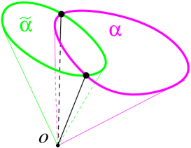
Figure 1: The image of the intersecting noncompact two cycles. The whole space expresses the singular Calabi-Yau manifold $X$ and the origin $O$ is the singularity. The radial direction expresses the $\phi$ and $Y$ direction, along which all the B-type D-branes spread. The cones $\alpha$ and $\tilde{\alpha}$ express the D-branes. Since they intersect at a surface ${\mathbb{C}}^{\times}$ of $\phi$ and $Y$, the intersection number is indefinite. This is the reason why we got the intersection number $0$. If we restrict to the section of the cycles (the base of the cone), the intersection number of this section in the manifold $X/{\mathbb{C}}^{\times}$ is possibly definite. We claim that the nontrivial factor of the open string Witten index corresponds to this intersection pairing in $X/{\mathbb{C}}^{\times}$

Let us consider a simple case that $X$ is written as

$$z_{1}^{N}+z_{2}^{N}+\dots+z_{n+1}^{N}=0\text{ in }{\mathbb{C}}^{n+1}.$$

When one notes the fact ${\mathbb{C}}P^{n}\cong({\mathbb{C}}^{n+1}-\{0\})/{\mathbb{C}}^{\times}$, the $X/{\mathbb{C}}^{\times}$ in our case turns out to be a Ricci positive $(n-1)$-fold in ${\mathbb{C}}P^{n}$. Moreover, we concentrate to the boundary states with $L=S=0$ to simplify our analyses. Also we may set $\zeta_{\alpha}=1$ in Eq.(3.2) because the Cardy condition is satisfied even for that case. In this case, the boundary states are labelled only by the index $M$. Then we can write down a nontrivial factor of the open string Witten index in the B-type case explicitly

$$\hat{I}_{M\tilde{M}} =\sum_{m_{1}^{\prime},\dots,m_{r}^{\prime}=0,\dots,2N}\delta^{{\rm mod}\;2N}_{M-\tilde{M}+\sum_{j}(m_{j}^{\prime}+1)}\left(\prod_{j=1}^{r}N_{0,0}^{m_{j}-1}\right)$$

$$=\sum_{m_{1}^{\prime},\dots,m_{r}^{\prime}=0,\dots,2N}\delta^{{\rm mod}\;2N}_{M-\tilde{M}+\sum_{j}(m_{j}^{\prime}+1)}\prod_{j=1}^{r}\left(\delta_{m_{j}^{\prime},1}-\delta_{m_{j}^{\prime},2N-1}\right)\,.$$

Because $M$ and $\tilde{M}$ should be even integers, we can introduce integers $a,b$ ($a,b=0,1,\dots,N-1$) as $a=M/2$ and $b=\tilde{M}/2$. The $\hat{I}$ is represented in a compact formula

$$\hat{I}_{a,b} =\sum_{c=0}^{r}\delta^{{\rm mod}\;N}_{a-b+c}\binom{r}{c}(-1)^{r-c}$$

$$=(-1)^{r}\sum_{m\geq 0}\binom{r}{b-a+mN}(-1)^{b-a+mN}\,.$$

It depends on only variables $a$ and $b$ and is interpreted as a $N\times N$ matrix $I_{G}$

$$I_{G}=(g^{-1}-1)^{r}\,,\,\,\,g^{N}=1\,.$$ (3.4)

Here the shift matrix $g$ is represented as an matrix with $N\times N$ entries

$$g=\left(\begin{matrix}0&1&&&&\cr&0&1&&&\cr&&0&1&&\cr&&&\ddots&\ddots&\cr&&&&0&1\cr 1&0&0&\cdots&0&0\cr\end{matrix}\right)\,.$$

The pairing obtained here is neither symmetric nor anti-symmetric with respect to two indices. We discuss the (anti-)symmetric part of this pairing. We consider the (anti-)symmetric part of $I_{G}$ as

$${I_{\blacklozenge}}:=-[I_{G}^{t}+(-1)^{r-1}I_{G}],$$

then, ${I_{\blacklozenge}}$ can be written as

$${I_{\blacklozenge}}=(g^{-1}-1)^{r}(g^{r-N}-1).$$ (3.5)

This is interpreted as follows.

In an ordinary compact Gepner model written by the Landau-Ginzburg model with a superpotential

$$W=z_{0}^{N_{0}}+z_{1}^{N_{1}}+\dots+z_{r}^{N_{r}},$$

the intersection form of B-type cycles becomes[2, 13]

$$I_{L=\tilde{L}=0}=\prod_{j}(g^{-K/N_{j}}-1),\quad K={\rm lcm}(N_{j}).$$

According to the paper [26], if we formally apply this formula to our case with a negative and fractional power part

$$W=z_{0}^{-N/(r-N)}+z_{1}^{N}+\dots+z_{r}^{N},$$

then (3.5) is obtained.

We compare these results with a calculation of an intersection pairing in terms of geometrical methods in the next section.

4 Geometric interpretation

In this section, we analyze topological properties of the manifold $M=X/{\mathbb{C}}^{\times}$ discussed in the previous section. The study here is based on geometrical methods and we compare results of intersection pairings obtained from two different approaches. It confirms the validity of our boundary states we constructed in the CFT.

4.1 Intersection pairing

In this section, we interpret the results in the Gepner model geometrically. First we take a Ricci positive $d=n-1$ dimensional manifold $M=X/{\mathbb{C}}^{\times}$

$$M\,;\,z_{1}^{N}+z_{2}^{N}+\cdots+z_{r}^{N}=0\qquad\mbox{in}\,\,\,{\mathbb{C}}P^{r-1}\,,$$

$$r=d+2=n+1\,.$$

Its first Chern class is evaluated by using a cohomology element $H\in H^{2}(M)$

$$c_{1}(TM)=(r-N)H\,.$$

Because M is realized as a zero locus of an ambient space $V={\mathbb{C}}P^{r-1}$, we can discuss topological properties of $M$ by analyzing characteristic classes of $V$ through a restriction on $M$. Our results in the previous sections are based on the analyses of open strings in the Gepner model and the associated objects “D-branes”(susy cycles) are expected to play important roles in our theory. A suitable basis for D-branes in the orbifold point[27, 28, 29, 30, 31, 32] is a set of line bundles (coherent sheaves) $\{{\cal O}(-a)\}$ $(a=0,1,2,\cdots,r-1)$ over $V$. (Associated analyses based on the Landau-Ginzburg models are performed in papers[33, 34, 35, 36]. Also applications to ${\cal N}=2$ gauge theories are proposed in papers[37, 26, 38].) The cylinder amplitude is interpreted as an index of the Dirac operator with boundary gauge bundles $(E,E^{\prime})$. In other words, it is a natural inner product on these bundles and is expressed as a relative Euler characteristic $\chi_{V}(E,E^{\prime})$ over $V$ (for $E={\cal O}(-a)$, $E^{\prime}={\cal O}(-b)$)

$$\langle{\cal O}(-a),{\cal O}(-b)\rangle_{V}:=\chi_{V}({\cal O}(-a),{\cal O}(-b))$$

$$\qquad=\int_{V}\mbox{ch}({\cal O}(-a)^{\ast})\mbox{ch}({\cal O}(-b))\mbox{Td}(TV)$$

$$\qquad=\left(\begin{matrix}r-1+a-b\\ a-b\end{matrix}\right)=:I_{a,b}\,,$$ (4.1)

$$\qquad\qquad(0\leq a\leq r-1\,;\,0\leq b\leq r-1)\,,$$

$$\mbox{Td}(TV)=\left(\frac{H}{1-e^{-H}}\right)^{r}\,.$$

From now on, we use an abbreviated notation $R_{a}$ for ${\cal O}(-a)$ $(a=0,1,\cdots,r-1)$.

Next we construct the dual basis $\{S^{a}\}$ of the $\{R_{a}\}$ $(0\leq a\leq r-1)$ as

$$\mbox{ch}({S^{a}})^{\ast}:=\sum_{b}(I^{-1})_{a,b}\mbox{ch}(R_{b})^{\ast}=\sum_{b}(-1)^{a-b}\left(\begin{matrix}r\cr a-b\end{matrix}\right)\mbox{ch}(R_{b})^{\ast}\,,$$

They satisfy orthonormal conditions with respect to the intersection pairing

$$\langle S^{a},R_{b}\rangle_{V}=\chi_{V}(S^{a},R_{b})=\chi_{V}({S^{a}}^{\ast}\otimes R_{b})=\delta^{a}{}_{b}\,.$$

The set of line bundles $\{{\cal O}(a)\}$ $(a=0,1,\cdots,r-1)$ is a strongly exceptional collection of the $V={\mathbb{C}}P^{r-1}$ and turns out to be a foundation of an associated helix of $V$. We can introduce an operation “left mutation ${\bf L}$” on the set $\{{\cal O}(a)\}$ as exact sequences

$$0\rightarrow\mbox{Ext}^{0}({\cal O}(a-1),{\cal O}(a))\otimes{\cal O}(a-1)\rightarrow{\cal O}(a)\rightarrow{\bf L}_{{\cal O}(a-1)}({\cal O}(a))\rightarrow 0\,,$$ (4.2)

or

$$0\rightarrow{\bf L}_{{\cal O}(a-1)}({\cal O}(a))\rightarrow\mbox{Ext}^{0}({\cal O}(a-1),{\cal O}(a))\otimes{\cal O}(a-1)\rightarrow{\cal O}(a)\rightarrow 0\,.$$ (4.3)

Here we used a condition $\mbox{Ext}^{0}({\cal O}(a-1),{\cal O}(a))=H^{0}({\cal O}(a-1),{\cal O}(a))\neq 0$ for $V$. It induces a relation of Chern characters of the bundles

$$\pm\mbox{ch}({\bf L}_{a-1}{\cal O}(a))=\mbox{ch}({\cal O}(a))-\chi_{V}({\cal O}(a-1),{\cal O}(a))\mbox{ch}({\cal O}(a-1))\,,$$ (4.4)

where we introduced a notation ${\bf L}_{a-1}{\cal O}(a)={\bf L}_{{\cal O}(a-1)}{\cal O}(a)$. The sign in Eq.(4.4) depends on the choice of sequences Eqs.(4.2),(4.3), that is to say, $(+)$ for Eq.(4.2), $(-)$ for Eq.(4.3). By using Eq.(4.4) iteratively, we can reexpress the ${S^{a}}^{\ast}$ as

$$\mbox{ch}(S^{a})^{\ast}=\sum^{a}_{b=0}(-1)^{a-b}\left(\begin{matrix}r\cr a-b\end{matrix}\right)\mbox{ch}({\cal O}(b))=\mbox{ch}({\bf L}_{0}{\bf L}_{1}\cdots{\bf L}_{a-1}{\cal O}(a))\,.$$ (4.5)

Namely, each element of ${S^{a}}^{\ast}$ can be constructed by acting left mutations on the $R_{a}^{\ast}={\cal O}(a)$.

Next we will take an equivalence class ${\cal O}(-[a])$ for $\{{\cal O}(-a)\}$ because $M$ has an extra cyclic property ${\mathbb{Z}}_{N}$ at the orbifold point

$${\cal O}(-[a+N])={\cal O}(-[a])\,.$$

The $[a]$ is defined modulo $N$. Equivalently we can interpret the number $a$ as an element of a cyclic group ${\mathbb{Z}}_{N}$. We shall write these elements of equivalence classes in an abbreviated form $R_{[a]}={\cal O}(-[a])$ $(a=0,1,\cdots,N-1)$.

In the previous sections, we investigate the boundary states in the Gepner model. Generally open strings can end on susy cycles described by homology cycles. When one discusses boundary states, homology classes play essential roles. An important class of topological invariants is an intersection pairing of homology cycles. These are related with cylinder amplitudes of open strings with boundary gauge bundles or sheaves. Now we define a pairing $\langle R_{[a]},R_{[b]}\rangle$ on these bundles on $M$

$${\bf I}_{a,b}:=\langle R_{[a]},R_{[b]}\rangle:=\sum_{\ell\geq 0}\sum_{m\geq 0}\int_{M}\mbox{ch}(R_{a+N\ell})^{\ast}\mbox{ch}(R_{b+Nm})\mbox{Td}(TM)\,,$$ (4.6)

$$\mbox{Td}(TM)=\left(\frac{H}{1-e^{-H}}\right)^{r}\left(\frac{1-e^{-NH}}{NH}\right)\,.$$

After performing the sum with respect to $m$ in Eq.(4.6), we can rewrite the pairing as

$$\langle R_{[a]},R_{[b]}\rangle=\sum_{\ell\geq 0}\int_{M}\mbox{ch}(R_{a+N\ell})^{\ast}\mbox{ch}(R_{b})\frac{1}{1-e^{-NH}}\cdot\mbox{Td}(TM)$$

$$\qquad=\sum_{\ell\geq 0}\int_{V}\mbox{ch}(R_{a+N\ell})^{\ast}\mbox{ch}(R_{b})\mbox{Td}(TV)\,.$$

Here we used a relation $\int_{M}(\cdots)=\int_{V}NH\times(\cdots)$. Thus we obtain an expression for the pairing

$$\langle R_{[a]},R_{[b]}\rangle=\sum_{\ell\geq 0}\int_{V}\mbox{ch}(R_{a+N\ell})^{\ast}\mbox{ch}(R_{b})\mbox{Td}(TV)$$

$$\qquad=:\sum_{c=0}^{r-1}\delta^{{\rm mod}\;N}_{a,c}\int_{V}\mbox{ch}({\cal O}(-a)^{\ast})\mbox{ch}({\cal O}(-b))\mbox{Td}(TV)=\sum_{c=0}^{r-1}\delta^{{\rm mod}\;N}_{a,c}I_{c,b}\,,$$

$$\qquad\qquad(0\leq a\leq N-1\,;\,0\leq b\leq N-1)\,.$$

This definition is natural because a usual pairing $I_{a,b}=\langle{\cal O}(-a),{\cal O}(-b)\rangle_{V}$ on the set $\{{\cal O}(-a)\}$ $(a=0,1,\cdots,r-1)$ is defined as Eq.(4.1). Also the ${\bf I}_{a,b}$ depends on only difference $(a-b)$ and we will write this as ${\bf I}_{a-b}$. The ${\bf I}_{a-b}$ is generally neither symmetric nor anti-symmetric under exchanges of $a$ and $b$

$${\bf I}_{a-b}=(-1)^{r}{\bf I}_{b-a+N-r}\,.$$

Only for $c_{1}(TM)=0$ case, the ${\bf I}_{a-b}$ is either symmetric for $r=$even or anti-symmetric for $r=$odd. However we can construct an (anti-)symmetric pairing ${\cal I}_{a,b}$ from the ${\bf I}_{a,b}$

$${\cal I}_{a,b}:={\bf I}_{a,b}+(-1)^{r-1}{\bf I}_{b,a}$$

$$\qquad={\bf I}_{a-b}+(-1)^{r-1}{\bf I}_{b-a}\,,$$ (4.7)

$${\cal I}_{a,b}=(-1)^{r-1}{\cal I}_{b,a}\,.$$

In other words, this ${\cal I}_{a,b}$ can be considered as an (anti)symmetrized version of the ${\bf I}_{a,b}$, that is, symmetric for $r=$odd case, anti-symmetric for $r=$even case. Also the ${\cal I}_{a,b}$ is expressed by using characteristic classes

$${\cal I}_{a,b}=\sum_{\ell\geq 0}\sum_{m\geq 0}\int_{M}\mbox{ch}(R_{a+N\ell})^{\ast}\mbox{ch}(R_{b+Nm})\mbox{Td}(TM)\cdot(1-e^{-c_{1}(TM)})\,,$$

$$\qquad=\sum_{\ell\geq 0}\int_{V}\mbox{ch}(R_{a+N\ell})^{\ast}\mbox{ch}(R_{b})\mbox{Td}(TV)\cdot(1-e^{-(r-N)H})\,.$$

Next we introduce a dual basis $\{S^{[a]}\}$ of the $\{R_{[a]}\}$ $(a=0,1,\cdots,N-1)$

$$\mbox{ch}(S^{[a]})^{\ast}=\sum_{c=0}^{r-1}\delta^{{\rm mod}\;N}_{c,a}\mbox{ch}(S^{c})^{\ast}:=\sum_{\ell\geq 0}\mbox{ch}(S^{a+N\ell})^{\ast}\,.$$ (4.8)

They satisfy a set of orthonormal conditions

$$\langle S^{[a]},R_{[b]}\rangle=\chi_{V}(S^{[a]},R_{[b]})$$

$$\qquad=\sum_{c=0}^{r-1}\delta^{{\rm mod}\;N}_{c,a}\int_{V}\mbox{ch}(S^{c})^{\ast}\mbox{ch}(R_{b})\mbox{Td}(TV)$$

$$\qquad=\sum_{c=0}^{r-1}\delta^{{\rm mod}\;N}_{c,a}\delta_{c,b}=\delta^{{\rm mod}\;N}_{b,a}=\delta^{a}{}_{b}\,,$$

$$\langle R_{[a]},S^{[b]}\rangle=\chi_{V}(R_{[a]},S^{[b]})$$

$$\qquad=\sum_{c=0}^{r-1}\delta^{{\rm mod}\;N}_{c,a}\int_{V}\mbox{ch}(R_{c}^{\ast})\mbox{ch}(S^{b})\mbox{Td}(TV)$$

$$\qquad=\sum_{c=0}^{r-1}\delta^{{\rm mod}\;N}_{c,a}\delta_{c,b}=\delta^{{\rm mod}\;N}_{b,a}=\delta_{a}{}^{b}\,,$$

$$\qquad(0\leq a\leq N-1\,;\,0\leq b\leq N-1)\,.$$

Then we can evaluate a pairing for each pair of elements $S^{[a]}$, $S^{[b]}$ $(a,b=0,1,\cdots,N-1)$

$$\langle S^{[a]},S^{[b]}\rangle=\chi_{V}(S^{[a]},S^{[b]})$$

$$\qquad=\sum_{c=0}^{r-1}\delta^{{\rm mod}\;N}_{c,a}\int_{V}\mbox{ch}(S^{c})^{\ast}\mbox{ch}(S^{b})\mbox{Td}(TV)$$

$$\qquad=\sum_{c=0}^{r-1}\delta^{{\rm mod}\;N}_{a,c}(I^{-1})_{c,b}=\sum^{r}_{c=0}\delta^{{\rm mod}\;N}_{a,c}\left(\begin{matrix}r\cr c-b\end{matrix}\right)\cdot(-1)^{c-b}$$

$$\qquad=\sum_{m\geq 0}\left(\begin{matrix}r\cr a-b+Nm\end{matrix}\right)(-1)^{a-b+Nm}\,,$$ (4.9)

$$\qquad\qquad(0\leq a\leq N-1\,;\,0\leq b\leq N-1)\,.$$

On the other hand, we calculated another intersection matrix $I_{G}$ in Eq.(3.4) of boundary states in the Gepner model for this case

$$M\,;\,z_{1}^{N}+z_{2}^{N}+\cdots+z_{r}^{N}=0\qquad\mbox{in}\,\,\,{{\mathbb{C}}P}^{r-1}\,,$$

$$I_{G}=(g^{-1}-1)^{r}\,,\,\,\,g^{N}=1\,.$$

One can express each component of the $I_{G}{}^{t}$ in an $(a,b)$th entry

$$(I_{G})^{t}_{a,b}=(-1)^{r}\sum_{m\geq 0}\left(\begin{matrix}r\cr a-b+Nm\end{matrix}\right)(-1)^{a-b+Nm}\,,$$ (4.10)

$$\qquad(0\leq a\leq N-1\,;\,0\leq b\leq N-1)\,.$$

This result Eq.(4.10) coincides with that in the geometric intersection Eq.(4.9) up to an irrelevant overall sign. That is to say, the boundary states we have obtained are associated with equivalence classes of the bundles (sheaves) $\{S^{[a]}\}$ $(a=0,1,\cdots,N-1)$ in Eq.(4.8). However, these are neither symmetric nor anti-symmetric under the exchanges $(a,b)\rightarrow(b,a)$. So we shall consider symmetrized parts of them by using the symmetrized pairing in Eq.(4.7)

$$\langle S^{[a]},S^{[b]}\rangle_{\cal I}=\langle S^{[a]},S^{[b]}\rangle+(-1)^{r-1}\langle S^{[b]},S^{[a]}\rangle$$

$$\qquad=\sum^{r-1}_{c=0}\delta^{{\rm mod}\;N}_{a,c}\left(\begin{matrix}r\cr c-b\end{matrix}\right)\cdot(-1)^{c-b}+(-1)^{r-1}\sum^{r-1}_{c=0}\delta^{{\rm mod}\;N}_{b,c}\left(\begin{matrix}r\cr c-a\end{matrix}\right)\cdot(-1)^{c-a}$$

$$\qquad=\sum_{m\geq 0}\left(\begin{matrix}r\cr a-b+Nm\end{matrix}\right)(-1)^{a-b+Nm}+(-1)^{r-1}\sum_{m\geq 0}\left(\begin{matrix}r\cr b-a+Nm\end{matrix}\right)(-1)^{b-a+Nm}\,,$$

$$\qquad\qquad(0\leq a\leq N-1\,;\,0\leq b\leq N-1)\,.$$

with $\langle S^{[a]},S^{[b]}\rangle_{\cal I}=(-1)^{r-1}\langle S^{[b]},S^{[a]}\rangle_{\cal I}$. Then we can compare this result with the matrix ${{I_{\blacklozenge}}}$ and $I_{G}$ in Eq.(3.5)

$$I_{G}=(g^{-1}-1)^{r}\,,$$

$${I_{\blacklozenge}}=(g^{-1}-1)^{r}(g^{r-N}-1)=(-1)[I_{G}+(-1)^{r-1}I_{G}^{t}]\,,$$

$$(-1)^{r-1}({I_{\blacklozenge}})^{t}_{a,b}=(-1)^{r}[(I_{G})^{t}_{a,b}+(-1)^{r-1}(I_{G})_{a,b}]$$

$$=\sum_{m\geq 0}\left(\begin{matrix}r\cr a-b+Nm\end{matrix}\right)(-1)^{a-b+Nm}+(-1)^{r-1}\sum_{m\geq 0}\left(\begin{matrix}r\cr b-a+Nm\end{matrix}\right)(-1)^{b-a+Nm}\,,$$

with $({I_{\blacklozenge}})^{t}=(-1)^{r-1}{I_{\blacklozenge}}$. As a conclusion, the $(-1)^{r-1}({I_{\blacklozenge}})^{t}_{a,b}$ coincides with the $\langle S^{[a]},S^{[b]}\rangle_{\cal I}$ on $V$

$$(-1)^{r-1}({I_{\blacklozenge}})^{t}_{a,b}=\langle S^{[a]},S^{[b]}\rangle_{\cal I}\,,$$

$$\langle S^{[b]},S^{[a]}\rangle_{\cal I}=(-1)^{r-1}\langle S^{[a]},S^{[b]}\rangle_{\cal I}\,.$$

That is to say, we are able to interpret the symmetrized part of the pairings of the boundary states as those of the bundles $\{S^{[a]}\}$. In other words, a state $|\{L=0\};M=2a;S=0\rangle$ corresponds to a bundle (sheaf) ${S^{[a]}}^{\ast}$. Formally an arbitrary state in the Gepner model could be represented as some bundle E with $\mbox{ch}(E)=\sum_{a}q_{a}\mbox{ch}(S^{[a]})^{\ast}$. (See also references[27, 28, 29, 30, 31, 32] for compact Calabi-Yau cases.)

Our analyses are based on investigation of the geometric properties of $M$. But we started originally a singular Calabi-Yau manifold in the Gepner model. In the next section, we will explain relations between results in this subsection and those in the Calabi-Yau case.

4.2 Singular Calabi-Yau manifold

In this subsection, we study a singular Calabi-Yau $n$-fold ${\cal M}$ realized as a zero locus in a weighted projective space

$$(z_{0},z_{1},z_{2},\cdots,z_{r})\in{\mathbb{C}}P^{r}(-(r-N),1,1,\cdots,1)\,,$$

$${\cal M}\,;\,p=\mu_{0}{z}_{0}^{-u}+\mu_{1}{z}_{1}^{N}+\mu_{2}{z}_{2}^{N}+\cdots+\mu_{r}{z}_{r}^{N}+\mu_{P}\cdot\prod^{r}_{i=0}{z}_{i}\,,$$ (4.11)

$$u=\frac{N}{r-N}\,,\,\,\,r=n+1\,,$$

$$\mbox{Td}(T{\cal M})=\left(\frac{H}{1-e^{-H}}\right)^{r}\left(\frac{1-e^{-NH}}{NH}\right)\left(\frac{1-e^{-(r-N)H}}{(r-N)H}\right)\,.$$

In the context of local mirror symmetries, this singular Calabi-Yau manifold can be interpreted as a total space of a bundle ${\cal O}(-N)\otimes{\cal O}(-(r-N))$ over $V={\mathbb{C}}P^{r-1}$ and its toric data are encoded in a vector $\ell^{(0)}$

$$\ell^{(0)}=(-N,-(r-N),1,1,\cdots,1)\,.$$ (4.12)

The last term in Eq.(4.11) induces a deformation of the complex structure of the manifold and its moduli space is described by a set of periods $\Pi_{\rho}$’s. The $\Pi_{\rho}$’s are functions of a variable $w$;

$${w}=(-1)^{r}\cdot\frac{\displaystyle\mu_{0}^{r-N}\cdot\mu_{P}^{N}}{\displaystyle\prod^{r}_{i=1}\mu_{i}}\,,$$

and we can evaluate their behaviors near $w\sim 0$

$$K^{\prime}:=G.C.M.\{N,r-N\}\,,$$

$$\Pi_{\rho}\sim w^{\rho}\qquad(w\sim 0)\,,$$

$$\qquad\qquad\mbox{for}\,\,\,\rho=0,\frac{m_{1}}{N},\frac{m_{2}}{r-N}\,\,\mbox{and}\,\,\,\rho\neq\frac{m}{K^{\prime}}\,,$$

$$\qquad\qquad(1\leq m_{1}\leq N-1\,;\,1\leq m_{2}\leq r-N-1)\,,$$

$$\Pi_{\rho}\sim w^{\rho}\log w\,,\,\,\,w^{\rho}\qquad(w\sim 0)\,,$$

$$\qquad\qquad\mbox{for}\,\,\,\rho=\frac{m}{K^{\prime}}\,,\qquad(1\leq m\leq K^{\prime}-1)\,.$$

The total number of periods is $(r-1)$ and $(K^{\prime}-1)$ solutions have logarithmic behaviors near $w\sim 0$. Precise formulae of these periods are summarized in the appendix B.

In the previous sections, we investigate properties of this model at an orbifold point $\mu_{P}\sim 0$ based on the Gepner model. When we look at the set of periods, some set of these $\Pi_{\rho}$ (in the Cases I,II in the appendix B) are combined into a basis of a ${\mathbb{Z}}_{N}$ symmetry at the orbifold point $w=0$

$$\Pi_{m/N}(e^{2\pi i}w)=e^{2\pi i\frac{m}{N}}\Pi_{m/N}(w)\,,$$

$$\rho=\frac{m}{N}\qquad(m=0,1,2,\cdots,N-1)\,.$$

The ${\mathbb{Z}}_{N}$ action is diagonalized on this set and this is an appropriate basis to describe structures near the orbifold point in the moduli space. It corresponds to $N$ elements of the basis in the Gepner model we discussed in the section 3. Now we note that the limit $w\rightarrow 0$ is also realized when $\mu_{0}$ in ${\cal M}$ tends to zero. The parameter $\mu_{0}$ is a coefficient of the singular part $z_{0}^{-u}$ and this operation $\mu_{0}\rightarrow 0$ turns out to reduce ${\cal M}$ to $M$ formally. That is the reason why the geometric properties of $M$ appear at the orbifold point.

Next we continue these $\Pi_{\rho}$ $(\rho=\frac{m}{N}\,;\,m=1,2,\cdots,N-1)$ analytically in a large radius region and investigate their classical parts $\Pi^{cl}_{\rho}$. Because we want to clarify their geometrical properties, it is enough to restrict ourselves to these geometric parts $\Pi^{cl}_{\rho=m/N}$

$$\Pi^{cl}_{m}\equiv\Pi^{cl}_{\rho=m/N}:=\sum^{N-1}_{a=1}e^{-2\pi i\frac{am}{N}}Z(R_{[a]})\,,$$

$$Z(R_{[a]}):=\sum_{n\geq 0}Z(R_{a+Nn})\,,$$

$$Z(R_{b}):=\int_{M}\left[\mbox{ch}(R_{b})^{\ast}e^{-tH}\cdot\sqrt{\hat{A}(H)}\right]\,,$$

$$\hat{A}(H)=\mbox{Td}(TM)\cdot\mbox{Td}({\cal O}(-(r-N)))\,.$$

Here the Chern characters of bundles $R_{a}$ or equivalence classes $R_{[a]}$ appear naturally and these are combined into an appropriate basis to describe properties in the orbifold point. Also we show full formulae of the $\Pi_{\rho=m/N}$ in the appendix C.

Our results based on the CFT are completely satisfactory and have appropriate geometrical interpretations. But the singular Calabi-Yau manifold has vanishing cohomology elements indicated in the paper [22]. They are interpreted to be missing objects in the CFT calculation as pointed in [22, 23, 24]. Our analyses in the section 3 are based on the Gepner model and we do not have enough understanding of these vanishing elements. The study of them might be possible in the language of local mirror symmetries. But we do not touch on them and postpone investigations of these singular properties in a future work.

5 Conclusion

In this paper, we developed a method to construct the boundary states in terms of the Gepner-like description of a noncompact singular Calabi-Yau manifold. We realize the singular Calabi-Yau manifold as a product of the Liouville part, $S^{1}$ part and tensor products of minimal models.

First we analyzed boundary conditions that can be imposed on fields in the Liouville and $S^{1}$ sectors. There are consistent A-,B-type conditions but the Liouville field always must take a Neumann type condition. We find that this fact is reduced to the structure of the manifold $X$. It is represented as a ${\mathbb{C}}^{\times}$ fibration over $X/{\mathbb{C}}^{\times}$ and the ${\mathbb{C}}^{\times}$ part is extended in the noncompact direction. Also the model has a linear dilaton background and the Liouville field is necessarily extended in the noncompact direction. It is the reason why the boundary condition of the Liouville field are free (Neumann type) in this ${\mathbb{C}}^{\times}$ direction and it induces a trivial structure.

In section 3, we construct boundary states in the A-,B-type cases and calculate the open string Witten indices between the boundary states. In both cases, they have a trivial factor $\theta_{1}(\tau)$. It has its origin on the trivial structure of the ${\mathbb{C}}^{\times}$ direction. Also that is related with the Neumann type condition we impose on the Liouville field. In addition to this trivial factor, the indices have nontrivial factors. We can express these factors explicitly and analyze their geometrical properties. Especially they are related with B-type D-branes wrapping around the fibered space $(\text{cycle of }X/{\mathbb{C}}^{\times})\times_{\rm f}{\mathbb{C}}^{\times}$.

In this paper, we only treat the Neumann boundary condition for the linear dilaton, in other words, D-branes wrapped on noncompact cycles on the noncompact manifold. It remains an important problem whether we are able to consider the D-branes wrapped on compact cycles on the noncompact manifold i.e. vanishing cycles. To consider the vanishing cycles, we need to impose some Dirichlet-like boundary condition on the ${\cal N}=2$ Liouville theory in the noncompact direction. When one naively imposes a Dirichlet condition on the $\phi$, the boundary condition of stress tensor $T$ is broken. It makes the analysis of $\phi$ difficult and we do not touch on this problem in this paper.

In section 4, we compare the $\text{cycle of }X/{\mathbb{C}}^{\times}$ and the nontrivial factor of the open string Witten index of the B-type boundary states. They have suitable geometrical interpretations and associated Witten indices coincide with pairings of coherent sheaves of the manifold. That is to say, the boundary states constructed here are identified with the $S^{a}$’s (or equivalence classes $S^{[a]}$’s). It is analogous to the compact Calabi-Yau cases[27, 28, 29, 30, 31, 32]. However for the compact Calabi-Yau cases, ambient spaces play crucial roles in the interpretations of the states in the geometrical language. In these cases, coherent sheaves of the ambient spaces are related with the boundary states through restrictions on the hypersurfaces. In contrast, for our noncompact Calabi-Yau cases, the Ricci positive manifolds $M$ in the singular CY’s essentially encode information on geometrical properties of the boundary states. The noncompact direction controlled by the Liouville field $\phi$ seems to lead a trivial contribution to our analyses because we always take a Neumann type condition on the $\phi$. When we discard this trivial contribution associated with the $\phi$, the remaining parts could be understood from the geometric data of the $M$.

Our results based on the CFT are completely satisfactory and have appropriate geometrical interpretations. But the singular Calabi-Yau manifold has vanishing cohomology elements indicated in the paper [22]. They are interpreted to be missing objects in the CFT calculation as pointed in [22, 23, 24]. Our analyses in the section 3 are based on the Gepner model and we do not have enough understanding of these vanishing elements. In fact, we calculated the full open string Witten index between the boundary states and showed it is actually zero. The reason why the index vanishes seems to be that we treat the ${\cal N}=2$ Liouville theory as a free field theory and set the “cosmological constant” $\mu_{0}$ to $0$. The geometrical meaning of this is that the singularity is not deformed. In [25], it is proposed that if the Liouville potential term is treated appropriately, then nonzero intersection numbers could be obtained. But our analyses here are based on the CFT calculations at the Gepner point and it seems that we study models with the “cosmological constant” $\mu_{0}=0$. That is consistent with the result[25]. More precise studies of them might be possible in the language of local mirror symmetries. But we do not touch on them and postpone investigations of these singular properties in a future work.

After we had submitted this article in the hep-th archive, a paper [25] by T. Eguchi and Y. Sugawara appeared which discusses a subject related to this article.

Acknowledgement

The authors would like to thank Michihiro Naka, Masatoshi Nozaki, Yuji Satoh and Yuji Sugawara for useful discussions and comments. S.Y. would also like to thank the organizers (T. Eguchi et al) of the Summer Institute 2000 at Yamanashi, Japan, 7-21 August, 2000, where a part of this work is done.

The work of S.Y. is supported in part by the JSPS Research Fellowships for Young Scientists.

Appendix A.    Theta functions and characters

In this appendix A, we collect several notations and summarize properties of theta functions. We use the following notations in this paper;

$$\,{\bf e}\!\left[x\right]:=\exp(2\pi ix),$$

$$\delta^{{\rm mod}\;N}_{m}:=\begin{cases}1&(m\equiv 0\mod N),\\ 0&({\rm others}),\end{cases}$$

$$\delta^{{\rm mod}\;N}_{m,m^{\prime}}:=\delta^{{\rm mod}\;N}_{m-m^{\prime}},$$

where $m$ and $N$ are integers. A useful equation is satisfied for integers $m$ and $N$

$$\sum_{j\in{\mathbb{Z}}_{N}}\,{\bf e}\!\left[\frac{jm}{N}\right]=N\delta^{{\rm mod}\;N}_{m}.$$

A set of SU(2) classical theta functions are defined as

$$\Theta_{m,k}(\tau,z)=\sum_{n\in{\mathbb{Z}}}q^{k\left(n+\frac{m}{2k}\right)^{2}}y^{k\left(n+\frac{m}{2k}\right)},$$

with $q:=\,{\bf e}\!\left[\tau\right],y:=\,{\bf e}\!\left[z\right]$. The Jacobi’s theta functions are also defined in our convention

$$\theta_{1}(\tau,z):=i\sum_{n\in{\mathbb{Z}}}(-1)^{n}q^{\left(n-\frac{1}{2}\right)^{2}}y^{\left(n-\frac{1}{2}\right)},\theta_{2}(\tau,z):=\sum_{n\in{\mathbb{Z}}}q^{\left(n-\frac{1}{2}\right)^{2}}y^{\left(n-\frac{1}{2}\right)},$$

$$\theta_{3}(\tau,z):=\sum_{n\in{\mathbb{Z}}}q^{n^{2}}y^{n},\hskip 76.82234pt\theta_{4}(\tau,z):=\sum_{n\in{\mathbb{Z}}}(-1)^{n}q^{n^{2}}y^{n}.$$

The above two kinds of theta functions are related through a set of linear transformations

$$2\Theta_{0,2}=\theta_{3}+\theta_{4},\ 2\Theta_{1,2}=\theta_{2}+i\theta_{1},\ 2\Theta_{2,2}=\theta_{3}-\theta_{4},\ 2\Theta_{3,2}=\theta_{2}-i\theta_{1}.$$

The Dedekind $\eta$ function is represented as an infinite product

$$\eta(\tau):=q^{\frac{1}{24}}\prod_{n=1}^{\infty}(1-q^{n}).$$

The character $\chi_{s}(\tau,z),\ s=0,1,2,3$ of $\widehat{SO(d)}_{1}$ for $d/2\in 2{\mathbb{Z}}+1$ can be expressed as

$$\chi_{0}(\tau,z)=\frac{\theta_{3}(\tau,z)^{d/2}+\theta_{3}(\tau,z)^{d/2}}{2\eta(\tau)^{d/2}},\ \ \chi_{1}(\tau,z)=\frac{\theta_{2}(\tau,z)^{d/2}+(i\theta_{1}(\tau,z))^{d/2}}{2\eta(\tau)^{d/2}},$$

$$\chi_{2}(\tau,z)=\frac{\theta_{3}(\tau,z)^{d/2}-\theta_{3}(\tau,z)^{d/2}}{2\eta(\tau)^{d/2}},\ \ \chi_{3}(\tau,z)=\frac{\theta_{2}(\tau,z)^{d/2}-(i\theta_{1}(\tau,z))^{d/2}}{2\eta(\tau)^{d/2}}.$$

Next we introduce a character $\chi_{m}^{\ell,s}(\tau,z)$ of a Verma module $(\ell,m,s)$ in the level $(N-2)$ minimal model. This function has equivalence relations with respect to its indices

$$\chi_{m}^{\ell,s}=\chi_{m+2N}^{\ell,s}=\chi_{m}^{\ell,s+4}=\chi_{m+N}^{N-2-\ell,s+2}.$$

One can see an explicit form of this $\chi_{m}^{\ell,s}(\tau,z)$ in the paper[6].

Next we shall look at modular properties of these functions. They behave under the T transformation $\tau\rightarrow\tau+1$

$$\Theta_{m,k}(\tau+1,z)=\,{\bf e}\!\left[\frac{m^{2}}{4k}\right]\Theta_{m,k}(\tau,z),$$

$$\theta_{1}(\tau+1,z)=\,{\bf e}\!\left[\tfrac{1}{8}\right]\theta_{1}(\tau,z),\qquad\theta_{2}(\tau+1,z)=\,{\bf e}\!\left[\tfrac{1}{8}\right]\theta_{2}(\tau,z),$$

$$\theta_{3}(\tau+1,z)=\theta_{4}(\tau,z),\qquad\theta_{4}(\tau+1,z)=\theta_{3}(\tau,z),$$

$$\eta(\tau+1)=\,{\bf e}\!\left[1/24\right]\eta(\tau),$$

$$\chi_{s}(\tau+1,z)=\,{\bf e}\!\left[\frac{s^{2}}{8}-\frac{d}{48}\right]\chi_{s}(\tau,z),$$

$$\chi_{m}^{\ell,s}(\tau+1,z)=\,{\bf e}\!\left[\frac{\ell(\ell+2)}{4N}-\frac{m^{2}}{4N}+\frac{s^{2}}{8}-\frac{N-2}{8N}\right]\chi_{m}^{\ell,s}(\tau,z).$$

For the S transformation $\tau\rightarrow-1/\tau$, they have following modular properties

$$\Theta_{m,k}(-1/\tau,z/\tau)=\sqrt{-i\tau}\,{\bf e}\!\left[\frac{k}{4}\frac{z^{2}}{\tau}\right]\sum_{m^{\prime}\in{\mathbb{Z}}_{2k}}\frac{1}{\sqrt{2k}}\,{\bf e}\!\left[-\frac{mm^{\prime}}{2k}\right]\Theta_{m^{\prime},k}(\tau,z),$$

$$\theta_{1}(-1/\tau,z/\tau)=-i\sqrt{-i\tau}\,{\bf e}\!\left[\frac{1}{2}\frac{z^{2}}{\tau}\right]\theta_{1}(\tau,z),\qquad\theta_{2}(-1/\tau,z/\tau)=\sqrt{-i\tau}\,{\bf e}\!\left[\frac{1}{2}\frac{z^{2}}{\tau}\right]\theta_{4}(\tau,z),$$

$$\theta_{3}(-1/\tau,z/\tau)=\sqrt{-i\tau}\,{\bf e}\!\left[\frac{1}{2}\frac{z^{2}}{\tau}\right]\theta_{3}(\tau,z),\qquad\theta_{4}(-1/\tau,z/\tau)=\sqrt{-i\tau}\,{\bf e}\!\left[\frac{1}{2}\frac{z^{2}}{\tau}\right]\theta_{2}(\tau,z),$$

$$\eta(-1/\tau)=\sqrt{-i\tau}\eta(\tau),$$

$$\chi_{s}(-1/\tau,z/\tau)=\,{\bf e}\!\left[\frac{d}{4}\frac{z^{2}}{\tau}\right]\sum_{s^{\prime}=0}^{3}\frac{1}{2}\,{\bf e}\!\left[-\frac{d}{2}\frac{ss^{\prime}}{4}\right]\chi_{s^{\prime}}(\tau,z),$$

$$\chi_{m}^{\ell,s}(-1/\tau,z/\tau)=\,{\bf e}\!\left[\frac{N-2}{2N}\frac{z^{2}}{\tau}\right]\frac{1}{\sqrt{8N}}\sum_{\ell,m,s}^{\rm even}A_{\ell\ell^{\prime}}\,{\bf e}\!\left[-\frac{ss^{\prime}}{4}+\frac{mm^{\prime}}{2N}\right]\chi_{m^{\prime}}^{\ell^{\prime},s^{\prime}}(\tau,z),$$

$$A_{\ell\ell^{\prime}}=\sqrt{\frac{2}{N}}\sin\left[\pi\frac{(\ell+1)(\ell^{\prime}+1)}{N}\right].$$

Here the symbol $\sum_{\ell,m,s}^{\rm even}$ means sums for $(\ell,m,s)$ under conditions $\ell+m+s\equiv 0\mod 2$. Also we use the notation $f(\tau)$ for a function $f(\tau,z)$ of $\tau,z$ with substituting $z=0$.

The SU(2) fusion coefficients $N_{\ell_{1}\ell_{2}}^{\ell_{3}}$ for $\ell_{1},\ell_{2},\ell_{3}=0,1,\dots,N-2$ are calculated in the following form

$$N_{\ell_{1}\ell_{2}}^{\ell_{3}}=\begin{cases}1&(|\ell_{1}-\ell_{2}|\leq\ell_{3}\leq\min\{\ell_{1}+\ell_{2},2N-4-\ell_{1}-\ell_{2}\})\\ 0&(\text{others})\end{cases}.$$

We can extend this definition satisfied for all integer $\ell_{1},\ell_{2},\ell_{3}$ by using relations $N_{\ell_{1}\ell_{2}}^{\ell_{3}}=N_{\ell_{1}\ell_{2}}^{-\ell_{3}-2}=N_{\ell_{1}\ell_{2}}^{\ell_{3}+2N}.$ Then, the Verlinde formula

$$N_{\ell_{1}\ell_{2}}^{\ell_{3}}=\sum_{\ell=0}^{N-2}\frac{A_{\ell\ell_{1}}A_{\ell\ell_{2}}A_{\ell\ell_{3}}}{A_{0\ell}}$$

is satisfied.

Appendix B.    Periods near the orbifold point

We will write down periods $\Pi_{\rho}$ for the Calabi-Yau manifold ${\cal M}$ in the region near the orbifold point. These solutions are labelled by a variable $\rho$;

1. Case I ; $\rho=0$

   $$\Pi_{\rho}\equiv 1\,$$

2. Case II ; $\rho=\frac{s+1}{N}$ $(s=0,1,2,\cdots,N-2)$

   $${\Pi_{\rho}}=\sum_{m\geq 0}\frac{\displaystyle\left[\Gamma\left(m+\frac{s+1}{N}\right)\right]^{n+2}\times{w}^{m+\frac{s+1}{N}}}{\displaystyle\Gamma(Nm+s+1)\Gamma\left(m+1+\frac{s+1}{N}\right)\Gamma\left((r-N)m+\frac{r-N}{N}(s+1)\right)}\,,$$

3. Case III ; $\rho=\frac{s+1}{r-N}$ $(s=0,1,2,\cdots,r-N-2)$ and $\rho\neq\frac{m}{K^{\prime}}$

   $${\Pi_{\rho}}=\sum_{m\geq 0}\frac{\displaystyle\left[\Gamma\left(m+\frac{s+1}{r-N}\right)\right]^{n+2}\times{w}^{m+\frac{s+1}{r-N}}}{\displaystyle\Gamma((r-N)m+s+1)\Gamma\left(m+1+\frac{s+1}{r-N}\right)\Gamma\left(Nm+\frac{N}{r-N}(s+1)\right)}\,,$$

4. Case IV ; $\rho=\frac{s+1}{K^{\prime}}$ $(s=0,1,2,\cdots,K^{\prime}-2)$

   $${\Pi_{\rho}}=\log{w}\times\sum_{m\geq 0}\frac{\displaystyle\left[\Gamma\left(m+\frac{s+1}{K^{\prime}}\right)\right]^{n+2}\times{w}^{m+\frac{s+1}{K^{\prime}}}}{\Gamma(\frac{r-N}{K^{\prime}}(s+1)+(r-N)m)\Gamma\left(m+1+\frac{s+1}{K^{\prime}}\right)\Gamma\left(Nm+\frac{N}{K^{\prime}}(s+1)\right)}$$

   $$\qquad+\sum_{m\geq 0}\frac{\displaystyle\left[\Gamma\left(m+\frac{s+1}{K^{\prime}}\right)\right]^{n+2}\times{w}^{m+\frac{s+1}{K^{\prime}}}}{\Gamma(\frac{r-N}{K^{\prime}}(s+1)+(r-N)m)\Gamma\left(m+1+\frac{s+1}{K^{\prime}}\right)\Gamma\left(Nm+\frac{N}{K^{\prime}}(s+1)\right)}$$

   $$\times\Bigl{\{}(n+2)\Psi\left(\frac{s+1}{K^{\prime}}+m\right)-N\cdot\Psi\left(\frac{N}{K^{\prime}}(s+1)+Nm\right)$$

   $$\qquad-(r-N)\Psi\left(\frac{r-N}{K^{\prime}}(s+1)+(r-N)m\right)-\Psi\left(1+m+\frac{s+1}{K^{\prime}}\right)\Bigr{\}}\,.$$

We use solutions in the Cases I, II to discuss ${\mathbb{Z}}_{N}$ properties of the $M$. The solutions in the Case IV have logarithmic behaviors near the orbifold point.

Appendix C.    Periods in the large volume region

We summarize concrete formulae of the $\Pi_{\rho}$’s for $\rho=m/N$ $(m=1,2,\cdots,N-1)$ in the large volume region

$$\Pi_{\rho}=(2\pi i)^{r-1}\times{(r-N)}\sum^{N-1}_{a=1}e^{-2\pi i\rho a}$$

$$\qquad\times\sum_{n\geq 0}\int_{M}\left[\mbox{ch}(R_{a+Nn})^{\ast}e^{-tH}\cdot\sqrt{\hat{A}(H)}\cdot\sqrt{\hat{K}(-H)}\times\exp\left(\sum_{\ell\geq 2}(-H)^{\ell}x_{\ell}\right)\right]\,,$$

$$t=\frac{1}{2\pi i}\left[\log{z}+\sum_{m\geq 1}a(m){z}^{m}\right]\,,\qquad z=w^{-1}\,,$$

$$\hat{A}(H)=\left(\frac{\displaystyle\frac{H}{2}}{\displaystyle\sinh\frac{H}{2}}\right)^{r}\cdot\left(\frac{\displaystyle\sinh\frac{NH}{2}}{\displaystyle\frac{NH}{2}}\right)\cdot\left(\frac{\displaystyle\sinh\frac{(r-N)H}{2}}{\displaystyle\frac{(r-N)H}{2}}\right)\,,$$

$$\hat{K}(-H)=\exp\left[\sum^{\infty}_{\ell=1}\frac{\zeta(2\ell+1)}{2\ell+1}\cdot\left(\frac{H}{2\pi i}\right)^{2\ell+1}\times\{N^{2\ell+1}+(r-N)^{2\ell+1}-r\}\right]\,,$$

$$x_{\ell}=\frac{1}{(2\pi i)^{\ell}}\cdot\frac{1}{\ell!}\partial_{v}^{\ell}\log\left\{1+v\sum_{m\geq 1}\frac{a(m+v)}{\tilde{a}(v)}{z}^{m}\right\}_{v=0}\,,$$

$$a(m+v)=\frac{\displaystyle\Gamma(1+N(m+v))\Gamma(1+(r-N)(m+v))\Gamma(m+v)}{[\Gamma(1+m+v)]^{n+2}}\,,$$

$$\tilde{a}(v)=\frac{\displaystyle\Gamma(1+Nv)\Gamma(1+(r-N)v)}{[\Gamma(1+v)]^{r}}\,.$$

These encode information on bundles $R_{a}$ and their properties are discussed in section 4.

References

- [1] J. L. Cardy, “Boundary Conditions, Fusion Rules and The Verlinde Formula”, Nucl. Phys. B324 (1989) 581.
- [2] I. Brunner, M. R. Douglas, A. Lawrence and C. Römelsberger, “D-branes on the Quintic”, JHEP 0008 (2000) 015, [hep-th/9906200].
- [3] M. R. Douglas, “Topics in D-geometry”, Class. Quant. Grav. 17 (2000) 1057, [hep-th/9910170].
- [4] N. Ishibashi, “The Boundary and Crosscap States in Conformal Field Theories”, Mod. Phys. Lett. A4 (1989) 251.
- [5] D. Gepner, “Exactly Solvable String Compactifications on Manifolds of SU(N) Holonomy”, Phys. Lett. B199 (1987) 380.
- [6] D. Gepner, “Space-Time Supersymmetry in Compactified String Theory and Superconformal Models”, Nucl. Phys. B296 (1988) 757.
- [7] H. Ooguri, Y. Oz and Z. Yin, “D-branes on Calabi-Yau Spaces and Their Mirrors”, Nucl. Phys. B477 (1996) 407, [hep-th/9606112].
- [8] A. Recknagel and V. Schomerus, “D-branes in Gepner models”, Nucl. Phys. B531 (1998) 185, [hep-th/9712186].
- [9] A. Recknagel and V. Schomerus, “Boundary Deformation Theory and Moduli Spaces of D-branes”, Nucl. Phys. B545 (1999) 233, [hep-th/9811237].
- [10] M. Gutperle and Y. Satoh, “D-branes in Gepner Models and Supersymmetry”, Nucl. Phys. B543 (1999) 73, [hep-th/9808080].
- [11] M. Gutperle and Y. Satoh, “D0-branes in Gepner Models and N = 2 Black Holes”, Nucl. Phys. B555 (1999) 477, [hep-th/9902120].
- [12] R. E. Behrend, P. A. Pearce, V. B. Petkova and J.-B. Zuber, “Boundary Conditions in Rational Conformal Field Theories”, Nucl. Phys. B570 (2000) 525–589, [hep-th/9908036].
- [13] D.-E. Diaconescu and C. Römelsberger, “D-branes and Bundles on Elliptic Fibrations”, Nucl. Phys. B574 (2000) 245, [hep-th/9910172].
- [14] P. Kaste, W. Lerche, C. A. Lütken and J. Walcher, “D-branes on K3-fibrations”, Nucl. Phys. B582 (2000) 203, [hep-th/9912147].
- [15] E. Scheidegger, “D-branes on Some One- and Two-parameter Calabi-Yau Hypersurfaces”, JHEP 04 (2000) 003, [hep-th/9912188].
- [16] M. Naka and M. Nozaki, “Boundary states in Gepner models”, JHEP 0005 (2000) 027, [hep-th/0001037].
- [17] I. Brunner and V. Schomerus, “D-branes at Singular Curves of Calabi-Yau Compactifications”, JHEP 04 (2000) 020, [hep-th/0001132].
- [18] J. Fuchs, C. Schweigert and J. Walcher, “Projections in String Theory and Boundary States for Gepner Models”, Nucl. Phys. B588 (2000) 110, [hep-th/0003298].
- [19] A. Giveon, D. Kutasov and O. Pelc, “Holography for Non-Critical Superstrings”, JHEP 9910 (1999) 035, [hep-th/9907178].
- [20] T. Eguchi and Y. Sugawara, “Modular Invariance in Superstring on Calabi-Yau n-fold with A-D-E Singularity”, Nucl. Phys. B577 (2000) 3, [hep-th/0002100].
- [21] S. Mizoguchi, “Modular Invariant Critical Superstrings on Four-dimensional Minkowski Space Two-dimensional Black Hole”, JHEP 0004 (2000) 014, [hep-th/0003053].
- [22] S. Yamaguchi, “Gepner-like Description of a String Theory on a Noncompact Singular Calabi-Yau Manifold”, Nucl. Phys. B594 (2001) 190, [hep-th/0007069].
- [23] S. Mizoguchi, “Noncompact Gepner Models for Type II Strings on a Conifold and an ALE Instanton”, hep-th/0009240.
- [24] M. Naka and M. Nozaki, “Singular Calabi-Yau Manifolds and ADE Classification of CFTs”, hep-th/0010002.
- [25] T. Eguchi and Y. Sugawara, “D-branes in Singular Calabi-Yau n-fold and N=2 Liouville Theory”, hep-th/0011148.
- [26] W. Lerche, “On a Boundary CFT Description of Nonperturbative N=2 Yang-Mills Theory”, hep-th/0006100.
- [27] D.-E. Diaconescu and M. R. Douglas, “D-branes on Stringy Calabi-Yau Manifolds”, hep-th/0006224.
- [28] K. Sugiyama, “Comments on Central Charge of Topological Sigma Model with Calabi-Yau Target Space”, Nucl. Phys. B591 (2000) 701, [hep-th/0003166].
- [29] S. Hosono, “Local Mirror Symmetry and Type IIA Monodromy of Calabi-Yau Manifolds”, Adv. Theor. Math. Phys. 4 (2000) , [hep-th/0007071].
- [30] S. Govindarajan and T. Jayaraman, “ D-branes, Exceptional Sheaves and Quivers on Calabi-Yau Manifolds: From Mukai to McKay”, hep-th/0010196.
- [31] A. Tomasiello, “D-branes on Calabi-Yau Manifolds and Helices”, hep-th/0010217.
- [32] P. Mayr, “Phases of Supersymmetric D-branes on Kähler Manifolds and the McKay Correspondence”, hep-th/0010223.
- [33] K. Hori, A. Iqbal and C. Vafa, “D-branes and Mirror Symmetry”, hep-th/0005247.
- [34] S. Govindarajan, T. Jayaraman and T. Sarkar, “Worldsheet Approaches to D-branes on Supersymmetric Cycles”, Nucl. Phys. B580 (2000) 519, [hep-th/9907131].
- [35] S. Govindarajan and T. Jayaraman, “On the Landau-Ginzburg Description of Boundary CFTs and Special Lagrangian Submanifolds”, JHEP 07 (2000) 016, [hep-th/0003242].
- [36] S. Govindarajan, T. Jayaraman and T. Sarkar, “On D-branes from Gauged Linear Sigma Models”, Nucl. Phys. B593 (2001) 155, [hep-th/0007075].
- [37] W. Lerche, A. Lütken and C. Schweigert, “D-Branes on ALE Spaces and the ADE Classification of Conformal Field Theories”, hep-th/0006247.
- [38] J. Fuchs, P. Kaste, W. Lerche, C. Lütken, C. Schweigert and J. Walcher, “Boundary Fixed Points, Enhanced Gauge Symmetry and Singular Bundles on K3”, hep-th/0007145.