hep-th/0011019

Stretched strings and worldsheets with a handle

Youngjai Kiem, Dong Hyun Park, and Haru-Tada Sato

BK21 Physics Research Division and Institute of Basic Science, Sungkyunkwan University, Suwon 440-746, Korea

ABSTRACT

In the presence of the constant background NS two-form gauge field, we construct the worldsheet partition functions, bulk propagators and boundary propagators for the worldsheets with a handle and a boundary. We analyze the noncommutative $\phi^{3}$ field theory amplitudes that correspond to the general two-point insertions on the two-loop nonplanar vacuum bubble. By the direct string theory amplitude computations on the worldsheets with a handle, which reduce to the aforementioned field theory amplitudes in the decoupling limit, we find that the stretched string interpretation remains valid for the types of amplitudes in consideration. This completes the demonstration that the stretched string picture holds up in the general multiloop context.

1 Introduction

The noncommutative field theories resulting from a certain decoupling limit of the open string theory with the constant background NS two-form gauge field [1, 2] have an inherent nonlocality [3]. Such unconventional features as the UV/IR mixing in noncommutative field theories [4] have largely been attributed to it. From the underlying string theory point of view, the stretched string interpretation of [5] has been successfully applied to explain that character of noncommutative field theories. In particular, in [6], the original suggestion of [5] based on the one-loop analysis [7] was extended to the multiloop context for the amplitudes coming from the (non)planar external vertex insertions on planar vacuum diagrams. The main theme of this note is to extend the analysis to the case of the external insertions on nonplanar vacuum diagrams. We find that the stretched string interpretation can successfully be extended to the case in consideration.

The technical highlight of this note is the explicit construction of the worldsheet partition function and the propagators for the open string worldsheets with a handle attached, presented in Section 2. Our construction directly computes the (boundary) open string propagators as well as the (bulk) closed string propagators. In the Reggeon vertex formalism of [8], one computes the amplitudes and the propagators are read off from those expressions. In section 3, we present a field theory analysis covering all the two-point 1PI external insertions on the two-loop nonplanar vacuum bubble in the noncommutative $\phi^{3}$ theory. Armed with the results in section 2, we then compute the string theory amplitudes involving nonplanar worldsheets, and consider the field theory reduction of the string theory calculations; we demonstrate the validity of the stretched string interpretation for the amplitudes in consideration in the following sense. Typical two-loop vacuum bubbles in the noncommutative $\phi^{3}$ field theory are depicted in Fig. 1, a planar vacuum bubble and a nonplanar vacuum bubble. When extended to string theory diagrams by ‘thickening’ the Feynman diagrams, a nonplanar vacuum bubble corresponds to an open string worldsheet with a handle attached. As shown in Fig. 1, the nonplanar vacuum bubble can also be regarded as coming from the nonplanar one-loop amplitude with the external vertices connected. In this sense, the one-loop external momentum turns into an internal momentum that should be integrated over all values. Since the stretching of the open string is given by $\Delta X^{\mu}=\theta^{\mu\nu}p_{\nu}$, in the decoupling limit $\alpha^{\prime}\rightarrow 0$, the stretching length $\Delta X^{\mu}G_{\mu\nu}\Delta X^{\nu}$ (here $G_{\mu\nu}$ is the open string metric) for the external open string can be chosen to be larger than the string scale $\alpha^{\prime}$. However, as a loop momentum, the contribution to the amplitudes from the $\Delta X^{\mu}G_{\mu\nu}\Delta X^{\nu}<\alpha^{\prime}$ momentum regime should also be considered. What we show in section 3 is that this type of contribution always goes to zero in the decoupling limit $\alpha^{\prime}\rightarrow 0$. We note that the field theory results presented in section 3 are consistent with those of [10]. In fact, our string theory consideration shows that the analysis of [10] is natural from the underlying string theory point of view.

In section 4, we discuss our results and the possible applications.

Figure 1: Two two-loop vacuum bubbles in $\phi^{3}$ field theory are shown. The upper diagram is a planar vacuum bubble and the lower diagram is a nonplanar vacuum bubble. The ‘thickened’ version of the diagrams are also shown.

2 Worldsheet partition function and propagators

In this section, after reviewing the geometries of worldsheets with and without a handle, we construct the worldsheet partition functions and propagators. For the latter, appropriate forms for both bulk and boundary propagators are computed. Though the essential part of our analysis can be generalized to worldsheets with multiple handles, we restrict our attention only to the worldsheets with a single handle and a boundary, where a simple and explicit analysis is possible.

2.1 $g=b=1$ Worldsheets and partition functions

A useful way to construct an open string worldsheet is to start from a closed string worldsheet and to fold it by half. From here on, we denote the genus $g$ worldsheet with $b$ boundaries as $(gb)$ surface. In Fig. 2, one finds a schematic representation of the closed string $(20)$ worldsheet. As denoted in the figure, the canonical basis of homology cycles is given by $a_{\alpha}$ and $b_{\alpha}$ cycles where $\alpha=1$ and $2$, with the intersection parings

$$(a_{\alpha},a_{\beta})=(b_{\alpha},b_{\beta})~{}~{},~{}~{}(a_{\alpha},b_{\beta})=-(b_{\alpha},a_{\beta})=\delta_{\alpha\beta}~{}~{}\rightarrow J=\pmatrix{0_{2}&1_{2}\cr-1_{2}&0_{2}}~{}.$$ (2.1)

Here $0_{2}$ and $1_{2}$ denote the $2\times 2$ zero and identity matrices, respectively. Dual to these cycles, there exist two holomorphic (antiholomorphic) one-forms $\omega_{\alpha}$ ($\bar{\omega}_{\alpha}$) among the cohomology group elements. The period matrix $\tau$ and the normalization of these one-forms are given by

$$\oint_{a_{\alpha}}\omega_{\beta}=\delta_{\alpha\beta}~{}~{}~{},~{}~{}~{}\oint_{b_{\alpha}}\omega_{\beta}=\tau_{\alpha\beta}~{}.$$ (2.2)

Up to three loops, it is known that the moduli space of the worldsheets are parameterized by the symmetric period matrix without any redundancy.

Figure 2: Depending on how we fold a $(20)$ surface, either a $(03)$ surface or a $(11)$ surface is obtained. The various homology cycles of the $(20)$ surface are also depicted.

Two inequivalent open string worldsheets that can be obtained from $(20)$ worldsheet by folding are $(03)$ surface and $(11)$ surface, each corresponding to a planar two-loop vacuum bubble and a nonplanar two-loop vacuum bubble. To be precise, the folding operation is an orientation-reversing (anticonformal) involution map $I$ ($I^{2}={\rm identity}$) and we identify the point $p$ with its involution image $I(p)$. The fixed points under the involution correspond to worldsheet boundaries. When acting on homology cycles, $I$ is represented by a matrix

$$\pmatrix{a^{\prime}\cr b^{\prime}}=I\pmatrix{a\cr b}=\pmatrix{H&G\cr F&E}\pmatrix{a\cr b}$$ (2.3)

and it satisfies

$$IJI^{T}=-J~{}.$$ (2.4)

Among the period matrix elements, only the “even” sector under the involution $I$ survives the folding, namely,

$$\tau=(E\bar{\tau}+F)(G\bar{\tau}+H)^{-1},$$ (2.5)

which reduces the real six dimensional moduli space of $(20)$ surfaces to the real three dimensional moduli spaces of $(11)$ surfaces or $(03)$ surfaces.

¿From what follows, we will concentrate on $(11)$ surfaces. Therefore, when acting on the canonical homology cycles, the involution matrix $I$ can be written as

$$\pmatrix{a^{\prime}\cr b^{\prime}}=I\pmatrix{a\cr b}=\pmatrix{\sigma&0_{2}\cr 0_{2}&-\sigma}\pmatrix{a\cr b}~{}~{}~{},~{}~{}~{}\sigma\equiv\pmatrix{0&1\cr 1&0}~{}~{}~{},$$ (2.6)

which yields the period matrix of the form

$$\tau=\pmatrix{a+ib&ic\cr ic&-a+ib},$$ (2.7)

where $a$, $b$, $c$ are real numbers. Even if this basis is easier to visualize, for the further analysis, we find it much simpler to use a different basis for the homology cycles. With an $Sp(4,{\hbox{{\rm Z}\kern-3.99994pt\hbox{\rm Z}}})$ matrix $M$ (satisfying $MJM^{T}=J$ and thus preserving the intersection pairing), we change the basis into

$$\pmatrix{\tilde{a}\cr\tilde{b}}=M\pmatrix{a\cr b}=\pmatrix{D&C\cr B&A}\pmatrix{a\cr b}=\pmatrix{1&-1&0&0\cr 0&0&1&1\cr 0&0&1&0\cr 0&-1&0&0}\pmatrix{a_{1}\cr a_{2}\cr b_{1}\cr b_{2}}~{}.$$ (2.8)

When normalized in the new basis, the period matrix $\tilde{\tau}$ ($\tilde{\tau}=(A\tau+B)(C\tau+D)^{-1}$) and the involution matrix $\tilde{I}$ ($\tilde{I}=MIM^{-1}$) can be written as

$$\tau=\pmatrix{iT_{11}&\frac{1}{2}+iT_{12}\cr\frac{1}{2}+iT_{21}&iT_{22}}$$ (2.9)

and

$$I=\pmatrix{-1_{2}&0_{2}\cr-\sigma&1_{2}}~{},$$ (2.10)

where $T_{11}$, $T_{22}$ and $T_{12}=T_{21}$ are three real numbers. In (2.9) and (2.10), since we will stick to the new basis hereafter, we have dropped tildes denoting the cycles, period matrix, etc. , in this basis. When compared to the $(03)$ surfaces (in the canonical homology basis) where

$$\tau=\pmatrix{iT_{11}&iT_{12}\cr iT_{21}&iT_{22}}~{}~{}~{},~{}~{}~{}I=\pmatrix{-1_{2}&0_{2}\cr 0_{2}&1_{2}}~{},$$ (2.11)

we immediately note that the $(11)$ surfaces come from the nonplanar two-point (open string) vertex insertions on an annulus (worldsheet vertex separation given by $\Delta z=1/2+iT_{12}$), while the $(03)$ surfaces originate from the planar two-point (open string) vertex insertions with the vertex separation $\Delta z=iT_{12}$.

We first consider the case when there is no background NS two-form field. Our situation of interests is the setup where there are $N$ stack of parallel D$p$-branes. It is then known from Refs. [11, 12] that the partition function for $(11)$ surfaces with the period matrix (2.9) can be written as (up to an overall normalization factor)

$$Z_{(11)}=N\int dT_{11}dT_{22}dT_{12}\frac{|W(\tau)|}{({\rm det}~{}2\pi\alpha^{\prime}~{}{\rm Im~{}}\tau)^{(p+1)/2}}~{},$$ (2.12)

where

$$|W(\tau)|=\prod_{a=1}^{10}|\theta_{a}(0|\tau)|^{-2}$$

and $\theta_{a}$’s are the ten even Riemann theta functions for the (20) surfaces. Similarly the partition function for $(03)$ surfaces can be written in the same form as (2.12) with the period matrix (2.11). We note that the partition function (2.12) is valid only when the involution matrix $I$ in (2.3) has components $G=0$ and $H=-E=-1_{2}$. Clearly, both the involution matrices of (2.10) and (2.11) satisfy this requirement, unlike the case of (2.6).

The key issue is to study the modification of the partition function when we turn on the constant background NS two-form field ($B$). As was argued in Refs. [6, 13], the partition functions for the planar ($g=0$) worldsheets do not change at all (modulo the overall multiplication factor) as we turn on the $B$ field. However for the nonplanar worldsheets such as (11) surfaces, where there exist intersecting cycles, there are changes in the form of the partition function [8]; we instead have the following expression

$$Z_{(11)}=N\int dT_{11}dT_{22}dT_{12}\frac{|W(\tau)|}{\sqrt{{\rm det}~{}(2\pi\alpha^{\prime}~{}G_{\mu\nu}~{}{\rm Im~{}}\tau+\frac{i}{2}\theta_{\mu\nu}{\cal I})}}~{}.$$ (2.13)

The open string metric $G^{\mu\nu}$ and the noncommutativity parameter $\theta^{\mu\nu}$ are related to the corresponding closed string quantities via

$$G^{\mu\nu}=(g_{\mu\nu}+B_{\mu\nu})^{-1}_{S}~{}~{}~{},~{}~{}~{}\theta^{\mu\nu}=2\pi\alpha^{\prime}(g_{\mu\nu}+B_{\mu\nu})^{-1}_{A}~{},$$ (2.14)

where the subscripts $S$ and $A$ denote the symmetric and the antisymmetric parts of a matrix, respectively. The $2\times 2$ matrix ${\cal I}$ is the intersection matrix for the intersecting cycles that are present in the worldsheet

$${\cal I}=\pmatrix{0&1\cr-1&0}~{}.$$ (2.15)

In (2.13), the determinant is taken with respect to the $2(p+1)\times 2(p+1)$ matrix $2\pi\alpha^{\prime}~{}G_{\mu\nu}~{}{\rm Im~{}}\tau+\frac{i}{2}\theta_{\mu\nu}{\cal I}$; as such, when $B_{\mu\nu}=0$, the partition function (2.13) reduces to (2.12). As is clear from the mode expansion at the tree level [1] and one-loop worldsheet propagators [7], the zero mode parts of the string modes are what is affected by turning on the $B$ field. Furthermore, the knowledge of one-loop worldsheet propagator is enough to see that the two-loop partition function (2.13) is the correct one, as sketched in Appendix A.

2.2 Worldsheet propagators

The knowledge of the worldsheet partition function is helpful for the construction of the worldsheet propagators. We suppose that the $\theta_{\mu\nu}$ matrix is $2\times 2$ block-diagonalized by an appropriate choice of the target space coordinates. Then for each block with $\theta_{\mu~{}\mu+1}=\theta_{\mu}$ (for odd $\mu$), we can compute the inverse of the matrix $2\pi\alpha^{\prime}~{}G_{\mu\nu}~{}{\rm Im~{}}\tau+\frac{i}{2}\theta_{\mu\nu}{\cal I}$ involved in the partition function (2.13):

$$\pmatrix{2\pi\alpha^{\prime}{\rm Im~{}}\tau&\frac{i}{2}\theta_{\mu}{\cal I}\cr-\frac{i}{2}\theta_{\mu}{\cal I}&2\pi\alpha^{\prime}~{}{\rm Im~{}}\tau}^{-1}=\pmatrix{\tilde{T}_{\theta_{\mu}}^{-1}&-\frac{i}{2D_{\theta_{\mu}}}\theta_{\mu}{\cal I}\cr\frac{i}{2D_{\theta_{\mu}}}\theta_{\mu}{\cal I}&\tilde{T}_{\theta_{\mu}}^{-1}},$$ (2.16)

where we introduce

$$D_{\theta_{\mu}}=(2\pi\alpha^{\prime})^{2}(T_{11}T_{22}-T_{12}^{2})+\frac{1}{4}\theta_{\mu}^{2}~{}~{}~{},~{}~{}~{}\tilde{T}_{\theta_{\mu}}^{-1}=\frac{2\pi\alpha^{\prime}}{D_{\theta_{\mu}}}\pmatrix{T_{22}&-T_{12}\cr-T_{12}&T_{11}}~{}.$$ (2.17)

We note that the matrix in (2.16) is a matrix in the target space coordinate basis, while the basis of the matrix in (2.17) is the homology cycle basis.

For simplicity, we start our consideration from the case when the only nonzero component of the $B$-field is $B_{12}=B$. Furthermore, we suppose $2\pi\alpha^{\prime}=1$, the closed string metric $g_{\mu\nu}=\eta_{\mu\nu}$ and the open string metric is given by $G^{\mu\nu}=\eta^{\mu\nu}/(1+B^{2})$, which also implies that $\theta_{\mu}^{2}\equiv\theta^{12}\theta_{12}=B^{2}$. Under these conventions, we note that $D_{B}=T_{11}T_{22}-T_{12}^{2}+B^{2}/4$ and $D_{0}=T_{11}T_{22}-T_{12}^{2}$. For the $(03)$ surfaces, the propagators for $X=X^{1}$ and $Y=X^{2}$ are given by [6]

$$\langle X(z)X(z^{\prime})\rangle\!\!\! = \!\!\!G(z,z^{\prime})\!+\!\frac{1\!-\!B^{2}}{1\!+\!B^{2}}G(z,\bar{z^{\prime}})\!+\!\frac{2B^{2}}{1\!+\!B^{2}}{\rm Re~{}}\Omega_{\alpha}(\tilde{T}^{-1}_{0})^{\alpha\beta}{\rm Re~{}}\Omega_{\beta},$$ (2.18)

$$\langle Y(z)X(z^{\prime})\rangle\!\!\! = \!\!\!\frac{2B}{1\!+\!B^{2}}\left(\frac{1}{2\pi}\log\frac{E(z,\bar{z^{\prime}})}{\left(E(z,\bar{z^{\prime}})\right)^{*}}+2i{\rm Re~{}}\Omega_{\alpha}(\tilde{T}^{-1}_{0})^{\alpha\beta}{\rm Im~{}}\Omega_{\beta}~{}\right)~{},$$ (2.19)

where the function $G$ is defined as

$$G(z,z^{\prime})=-\frac{1}{2\pi}\log\left|E(z,z^{\prime})\right|^{2}+{\rm Im~{}}\Omega_{\alpha}(\tilde{T}^{-1}_{0})^{\alpha\beta}{\rm Im~{}}\Omega_{\beta}~{}.$$ (2.20)

The overbar on the worldsheet position denotes the involution transformed position $\bar{z}=I(z)$ of the position $z$. The indices $(\alpha,\beta)$ run over the $(1,2)$ homology cycles, $E(z,w|\tau)$ is the prime form on $(20)$ surface, and $\Omega_{\alpha}$ is the complex integral of the Abelian differential $\omega_{\alpha}$ from a point $\bar{z}^{\prime}$ to a point $z$ along a contractible path

$$\Omega_{\alpha}=\int_{\bar{z}^{\prime}}^{z}\omega_{\alpha}~{},$$ (2.21)

where the path passes through a reference point $P$ lying on one of the boundaries. We note that for a contractible path

$${\rm Im~{}}\int_{z^{\prime}}^{z}\omega_{\alpha}={\rm Im~{}}\int_{\bar{z}^{\prime}}^{z}\omega_{\alpha},$$ (2.22)

which explains why $G(z,z^{\prime})$ and $G(z,\bar{z}^{\prime})$ can be chosen to have the same quadratic pieces.

Figure 3: Various representations of a $(11)$ surface. The figure on the right side is the Schottky representation of a $(11)$ surface. The overbar on a cycle denotes the fact that the cycle is cut in half by the folding process. The bold lines represent the worldsheet boundary.

The main difference between the $(03)$ surfaces and $(11)$ surfaces is the existence of the intersecting cycles in the latter (see Fig. 3). In terms of the homology basis where the period matrix is of form (2.9), these cycles are written as

$${\rm a}=a_{1}-b_{2}~{}~{}~{},~{}~{}~{}{\rm b}=b_{1}$$ (2.23)

with the intersection matrix ${\cal I}$ given in (2.15). We note that ${\rm a}={\rm a_{1}}$ and ${\rm b}={\rm b_{1}}$ in Fig. 3. On top of the contractible path contribution to $\Omega_{\alpha}$, we should, in general, allow the contributions from the integration over a cycle of the form ${\rm c}=m{\rm a}+n{\rm b}$ (where $mn\neq 0$), which corresponds to a nonzero cycle of the homology group (see Fig. 4):

$$\Omega_{\alpha}=\Omega^{0}_{\alpha}+\Omega^{t}_{\alpha}\equiv\int_{\bar{z}^{\prime}}^{z}\omega_{\alpha}+\oint_{{\rm c}}\omega_{\alpha}~{}.$$ (2.24)

For $\Omega^{0}_{\alpha}$, the integral is taken over a contractible path, and the second term $\Omega^{t}_{\alpha}$ is a topological number that does not change as we locally move the positions $z$ and $z^{\prime}$.

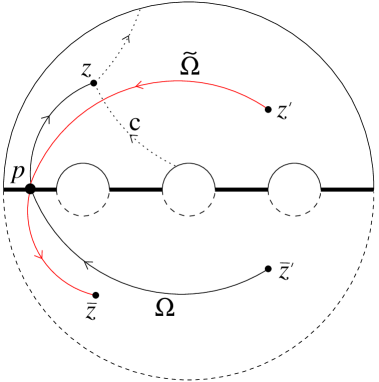
Figure 4: The integration path for $\Omega$ and $\tilde{\Omega}$ are shown in the Schottky representation. The paths are required to pass through a reference point $P$.

Since the worldsheet propagators should be well-defined over the whole worldsheet, we require that the $(11)$ propagators be invariant under the periodic shifts along the ${\rm p}={\rm a}$ and ${\rm p}={\rm b}$ cycles. Under these transformations, the various objects appearing in $(03)$ propagators in (2.18) and (2.19) change into:

$$\Delta\left\{-\frac{1}{2\pi}\log\left|E(z,z^{\prime})\right|^{2}\right\} = -2{\rm Im~{}}\Omega_{1}-T_{11}~{},$$ (2.25)

$$\Delta\left\{-\frac{1}{2\pi}\log\left|E(z,\bar{z}^{\prime})\right|^{2}\right\} = -2{\rm Im~{}}\Omega_{1}-T_{11}~{},$$ (2.26)

$$2\Delta\left\{{\rm Im~{}}\Omega_{\alpha}(\tilde{T}^{-1}_{B})^{\alpha\beta}{\rm Im~{}}\Omega_{\beta}\right\} = 4\frac{D_{0}}{D_{B}}{\rm Im~{}}\Omega_{1}+2\frac{D_{0}}{D_{B}}T_{11}~{},$$ (2.27)

$$2B^{2}\Delta\left\{{\rm Re~{}}\Omega_{\alpha}(\tilde{T}^{-1}_{B})^{\alpha\beta}{\rm Re~{}}\Omega_{\beta}\right\} = 2\frac{B^{2}}{D_{B}}(T_{11}{\rm Re~{}}\Omega_{2}-T_{12}{\rm Re~{}}\Omega_{1})+\frac{B^{2}}{2D_{B}}T_{11}~{},$$ (2.28)

$$\Delta\left\{\frac{1}{2\pi}\log\frac{E(z,\bar{z^{\prime}})}{\left(E(z,\bar{z^{\prime}})\right)^{*}}\right\} = -2i{\rm Re~{}}\Omega_{1}~{},$$ (2.29)

$$2i\Delta\left\{{\rm Re~{}}\Omega_{\alpha}(\tilde{T}^{-1}_{B})^{\alpha\beta}{\rm Im~{}}\Omega_{\beta}\right\} = \frac{i}{D_{B}}(T_{11}{\rm Im~{}}\Omega_{2}-T_{12}{\rm Im~{}}\Omega_{1})+2i\frac{D_{0}}{D_{B}}{\rm Re~{}}\Omega_{1}~{},$$ (2.30)

for the shifts along the ${\rm b}$-cycle and

$$\Delta\left\{-\frac{1}{2\pi}\log\left|E(z,z^{\prime})\right|^{2}\right\} = 2{\rm Im~{}}\Omega_{2}-T_{22}~{},$$ (2.31)

$$\Delta\left\{-\frac{1}{2\pi}\log\left|E(z,\bar{z}^{\prime})\right|^{2}\right\} = 2{\rm Im~{}}\Omega_{2}-T_{22}~{},$$ (2.32)

$$2\Delta\left\{{\rm Im~{}}\Omega_{\alpha}(\tilde{T}^{-1}_{B})^{\alpha\beta}{\rm Im~{}}\Omega_{\beta}\right\} = -4\frac{D_{0}}{D_{B}}{\rm Im~{}}\Omega_{2}+2\frac{D_{0}}{D_{B}}T_{22}~{},$$ (2.33)

$$2B^{2}\Delta\left\{{\rm Re~{}}\Omega_{\alpha}(\tilde{T}^{-1}_{B})^{\alpha\beta}{\rm Re~{}}\Omega_{\beta}\right\} = 2\frac{B^{2}}{D_{B}}(T_{22}{\rm Re~{}}\Omega_{1}-T_{12}{\rm Re~{}}\Omega_{2})+\frac{B^{2}}{2D_{B}}T_{22}~{},$$ (2.34)

$$\Delta\left\{\frac{1}{2\pi}\log\frac{E(z,\bar{z^{\prime}})}{\left(E(z,\bar{z^{\prime}})\right)^{*}}\right\} = +2i{\rm Re~{}}\Omega_{2}~{},$$ (2.35)

$$2i\Delta\left\{{\rm Re~{}}\Omega_{\alpha}(\tilde{T}^{-1}_{B})^{\alpha\beta}{\rm Im~{}}\Omega_{\beta}\right\} = i\frac{1}{D_{B}}(T_{22}{\rm Im~{}}\Omega_{1}-T_{12}{\rm Im~{}}\Omega_{2})-2i\frac{D_{0}}{D_{B}}{\rm Re~{}}\Omega_{2}~{},$$ (2.36)

for the shifts along the ${\rm a}$-cycle. We use the fact that $\Omega_{\alpha}$ in (2.24) transforms into $\Omega_{\alpha}+\oint_{\rm p}\omega_{\alpha}$, the prime form remains invariant under the $a$-cycle transformation and changes to

$$E(\pm b_{\alpha}(z),w|\tau)=-\exp\left[-2\pi i(\frac{1}{2}\tau_{\alpha\alpha}\pm\int_{w}^{z}\omega_{\alpha})\right]E(z,w|\tau)$$ (2.37)

under the ${\rm b}$-cycle shifts as can be derived from its modular transformation properties. Recalling the linear independence of ${\rm Re~{}}\Omega_{\alpha}$ and ${\rm Im~{}}\Omega_{\beta}$, we find that no combinations from (2.25) to (2.36) can satisfy the periodicity.

Other possible zero mode terms that we can add are the combinations involving the off-diagonal elements of (2.16) proportional to the intersection matrix ${\cal I}$. In particular, one can verify that

$$-B^{2}\Delta\left\{{\rm Re~{}}\tilde{\Omega}_{\alpha}\frac{1}{D_{B}}{\cal I}^{\alpha\beta}{\rm Im~{}}\Omega_{\beta}+{\rm Re~{}}\Omega_{\alpha}\frac{1}{D_{B}}{\cal I}^{\alpha\beta}{\rm Im~{}}\tilde{\Omega}_{\beta}\right\}$$

$$=-2\frac{B^{2}}{D_{B}}(T_{11}{\rm Re~{}}\Omega^{0}_{2}-T_{12}{\rm Re~{}}\Omega_{1}^{0})+\frac{B^{2}}{D_{B}}{\rm Im~{}}\Omega_{1}^{0}\equiv XX_{{\rm b}}(\Omega^{0})~{},$$ (2.38)

$$\frac{i}{2}\Delta\left\{{\rm Im~{}}\tilde{\Omega}_{\alpha}\frac{1}{D_{B}}{\cal I}^{\alpha\beta}{\rm Im~{}}\Omega_{\beta}-B^{2}{\rm Re~{}}\tilde{\Omega}_{\alpha}\frac{1}{D_{B}}{\cal I}^{\alpha\beta}{\rm Re~{}}\Omega_{\beta}\right\}$$

$$=-i\frac{1}{D_{B}}(T_{11}{\rm Im~{}}\Omega^{0}_{2}-T_{12}{\rm Im~{}}\Omega^{0}_{1})+i\frac{B^{2}}{2D_{B}}{\rm Re~{}}\Omega_{1}^{0}\equiv XY_{{\rm b}}(\Omega^{0})~{},$$ (2.39)

for the ${\rm b}$-cycle shift and

$$-B^{2}\Delta\left\{{\rm Re~{}}\tilde{\Omega}_{\alpha}\frac{1}{D_{B}}{\cal I}^{\alpha\beta}{\rm Im~{}}\Omega_{\beta}+{\rm Re~{}}\Omega_{\alpha}\frac{1}{D_{B}}{\cal I}^{\alpha\beta}{\rm Im~{}}\tilde{\Omega}_{\beta}\right\}$$

$$=-2\frac{B^{2}}{D_{B}}(T_{22}{\rm Re~{}}\Omega^{0}_{1}-T_{21}{\rm Re~{}}\Omega_{2}^{0})-\frac{B^{2}}{D_{B}}{\rm Im~{}}\Omega_{2}^{0}\equiv XX_{{\rm a}}(\Omega^{0})~{},$$ (2.40)

$$\frac{i}{2}\Delta\left\{{\rm Im~{}}\tilde{\Omega}_{\alpha}\frac{1}{D_{B}}{\cal I}^{\alpha\beta}{\rm Im~{}}\Omega_{\beta}-B^{2}{\rm Re~{}}\tilde{\Omega}_{\alpha}\frac{1}{D_{B}}{\cal I}^{\alpha\beta}{\rm Re~{}}\Omega_{\beta}\right\}$$

$$=-i\frac{1}{D_{B}}(T_{22}{\rm Im~{}}\Omega^{0}_{1}-T_{21}{\rm Im~{}}\Omega^{0}_{2})-i\frac{B^{2}}{2D_{B}}{\rm Re~{}}\Omega_{2}^{0}\equiv XY_{{\rm a}}(\Omega^{0})~{},$$ (2.41)

for the ${\rm a}$-cycle shift. Here, we introduce an object $\tilde{\Omega}_{\alpha}$ via the definition (see Fig. 4)

$$\tilde{\Omega}_{\alpha}=\tilde{\Omega}^{0}_{\alpha}+\tilde{\Omega}^{t}_{\alpha}\equiv\int_{z^{\prime}}^{\bar{z}}\omega_{\alpha}-\oint_{I({\rm c})}\omega_{\alpha}~{}.$$ (2.42)

In line with the flipped sign for the topological term in comparison to (2.24), $\tilde{\Omega}_{\alpha}$ shifts to $\tilde{\Omega}_{\alpha}-\oint_{I({\rm p})}\omega_{\alpha}$ under a ${\rm p}$-cycle shift. One can verify that the following “parity” rule holds:

$${\rm Re~{}}\tilde{\Omega}^{0}_{\alpha}=-{\rm Re~{}}\Omega^{0}_{\alpha}~{}~{}~{},~{}~{}~{}{\rm Im~{}}\tilde{\Omega}^{0}_{\alpha}={\rm Im~{}}\Omega^{0}_{\alpha}~{}~{}~{},~{}~{}~{}{\rm Re~{}}\tilde{\Omega}^{t}_{\alpha}={\rm Re~{}}\Omega^{t}_{\alpha}~{}~{}~{},~{}~{}~{}{\rm Im~{}}\tilde{\Omega}^{t}_{\alpha}=-{\rm Im~{}}\Omega^{t}_{\alpha}~{}.$$ (2.43)

For cycles of the form ${\rm c}=m{\rm a}+n{\rm b}$ in (2.24) where $m$ and $n$ are integers and for these cycles only, using the explicit computation

$$\oint_{{\rm a}}\omega_{\alpha}=\pmatrix{\frac{1}{2}-iT_{12}\cr-iT_{22}}~{}~{}~{},~{}~{}~{}\oint_{{\rm b}}\omega_{\alpha}=\pmatrix{iT_{11}\cr\frac{1}{2}+iT_{12}}~{},$$ (2.44)

it is straightforward to verify that

$$XX_{{\rm b}}(\Omega^{0})=XX_{{\rm b}}(\Omega)~{}~{}~{},~{}~{}~{}XY_{{\rm b}}(\Omega^{0})=XY_{{\rm b}}(\Omega)-im~{}~{}~{},$$ (2.45)

for the objects in (2.38) and (2.39) originating from the ${\rm b}$-cycle shift and

$$XX_{{\rm a}}(\Omega^{0})=XX_{{\rm a}}(\Omega)~{}~{}~{},~{}~{}~{}XY_{{\rm a}}(\Omega^{0})=XY_{{\rm a}}(\Omega)+in~{}~{}~{},$$ (2.46)

for the objects in (2.40) and (2.41) coming from the ${\rm a}$-cycle shift. We note that the function $\frac{1}{2\pi}\log\frac{E(z,\bar{z^{\prime}})}{\left(E(z,\bar{z^{\prime}})\right)^{*}}$ has branch cuts since it is defined only modulo $i{\hbox{{\rm Z}\kern-3.99994pt\hbox{\rm Z}}}$. Therefore by making an appropriate branch choice, we can cancel the extra integer terms in (2.45) and (2.46).

Collecting the results of the analysis so far and recalling that the effect of the constant $B$ field affects only the zero mode parts, we can immediately write down the following periodic worldsheet propagators for $(11)$ surfaces:

$$\langle X(z)X(z^{\prime})\rangle\!\!\! = \!\!\!G(z,z^{\prime})\!+\!\frac{1\!-\!B^{2}}{1\!+\!B^{2}}G(z,\bar{z^{\prime}})\!+\!\frac{2B^{2}}{1\!+\!B^{2}}{\rm Re~{}}\Omega_{\alpha}(\tilde{T}^{-1}_{B})^{\alpha\beta}{\rm Re~{}}\Omega_{\beta}$$ (2.47)

$$-\frac{B^{2}}{1+B^{2}}\left({\rm Re~{}}\tilde{\Omega}_{\alpha}\frac{1}{D_{B}}{\cal I}^{\alpha\beta}{\rm Im~{}}\Omega_{\beta}+{\rm Re~{}}\Omega_{\alpha}\frac{1}{D_{B}}{\cal I}^{\alpha\beta}{\rm Im~{}}\tilde{\Omega}_{\beta}\right)~{},$$

$$\langle Y(z)X(z^{\prime})\rangle\!\!\! = \!\!\!\frac{2B}{1\!+\!B^{2}}\left(\frac{1}{2\pi}\log\frac{E(z,\bar{z^{\prime}})}{\left(E(z,\bar{z^{\prime}})\right)^{*}}+2i{\rm Re~{}}\Omega_{\alpha}(\tilde{T}^{-1}_{B})^{\alpha\beta}{\rm Im~{}}\Omega_{\beta}~{}\right)$$ (2.48)

$$+i\frac{B}{1+B^{2}}\left({\rm Im~{}}\tilde{\Omega}_{\alpha}\frac{1}{D_{B}}{\cal I}^{\alpha\beta}{\rm Im~{}}\Omega_{\beta}-B^{2}{\rm Re~{}}\tilde{\Omega}_{\alpha}\frac{1}{D_{B}}{\cal I}^{\alpha\beta}{\rm Re~{}}\Omega_{\beta}\right)~{},$$

where the function $G$ is defined as

$$G(z,z^{\prime})=-\frac{1}{2\pi}\log\left|E(z,z^{\prime})\right|^{2}+{\rm Im~{}}\Omega_{\alpha}(\tilde{T}^{-1}_{B})^{\alpha\beta}{\rm Im~{}}\Omega_{\beta}~{}.$$ (2.49)

Using (2.43), we can rewrite

$$-\frac{B^{2}}{1+B^{2}}\left({\rm Re~{}}\tilde{\Omega}_{\alpha}\frac{1}{D_{B}}{\cal I}^{\alpha\beta}{\rm Im~{}}\Omega_{\beta}+{\rm Re~{}}\Omega_{\alpha}\frac{1}{D_{B}}{\cal I}^{\alpha\beta}{\rm Im~{}}\tilde{\Omega}_{\beta}\right)$$

$$=\frac{2B^{2}}{1+B^{2}}\left({\rm Re~{}}\Omega^{0}_{\alpha}\frac{1}{D_{B}}{\cal I}^{\alpha\beta}{\rm Im~{}}\Omega^{t}_{\beta}-{\rm Re~{}}\Omega^{t}_{\alpha}\frac{1}{D_{B}}{\cal I}^{\alpha\beta}{\rm Im~{}}\Omega^{0}_{\beta}\right)~{},$$ (2.50)

and

$$i\frac{B}{1+B^{2}}\left({\rm Im~{}}\tilde{\Omega}_{\alpha}\frac{1}{D_{B}}{\cal I}^{\alpha\beta}{\rm Im~{}}\Omega_{\beta}-B^{2}{\rm Re~{}}\tilde{\Omega}_{\alpha}\frac{1}{D_{B}}{\cal I}^{\alpha\beta}{\rm Re~{}}\Omega_{\beta}\right)$$

$$=i\frac{2B}{1+B^{2}}\left({\rm Im~{}}\Omega^{0}_{\alpha}\frac{1}{D_{B}}{\cal I}^{\alpha\beta}{\rm Im~{}}\Omega^{t}_{\beta}+B^{2}{\rm Re~{}}\Omega^{0}_{\alpha}\frac{1}{D_{B}}{\cal I}^{\alpha\beta}{\rm Re~{}}\Omega^{t}_{\beta}\right)~{}.$$ (2.51)

Noting that the part

$$\frac{2B^{2}}{1\!+\!B^{2}}{\rm Re~{}}\Omega_{\alpha}(\tilde{T}^{-1}_{B})^{\alpha\beta}{\rm Re~{}}\Omega_{\beta}$$ (2.52)

from (2.47) and the part

$$i\frac{4B}{1+B^{2}}{\rm Re~{}}\Omega_{\alpha}(\tilde{T}^{-1}_{B})^{\alpha\beta}{\rm Im~{}}\Omega_{\beta}$$ (2.53)

from (2.48) satisfy the boundary conditions [6], we see that (2.50) and (2.51) parts also satisfy the boundary conditions.

Given the expression for the bulk worldsheet propagators, one can construct the boundary propagators by considering the factorization of the string amplitudes, for example, as sketched in [6] for the $(03)$ surfaces. In this process, one should be careful to include the effects of self-contractions. The position of the boundary is the line where ${\rm Re~{}}\Omega^{0}_{\alpha}=0$, recalling that ${\rm Re~{}}\Omega^{0}_{\alpha}\rightarrow-{\rm Re~{}}\Omega^{0}_{\alpha}$ under the involution and there is a single boundary for the $(11)$ surfaces. Therefore ${\rm Re~{}}\Omega_{\alpha}$ consists of purely topological term ${\rm Re~{}}\Omega^{t}_{\alpha}$. The covariant form of the boundary propagator thus obtained is as follows:

$$G^{\mu\nu}_{\rm open}(z,z^{\prime}) = \alpha^{\prime}G^{\mu\nu}G(z,z^{\prime})$$

$$+(\theta G\theta)^{\mu\nu}\left({\rm Re~{}}\Omega^{t}_{\alpha}(\tilde{T}^{-1}_{\theta})^{\alpha\beta}{\rm Re~{}}\Omega^{t}_{\beta}+(2\pi\alpha^{\prime})~{}{\rm Re~{}}\Omega^{t}_{\alpha}(\frac{1}{D_{\theta}}{\cal I})^{\alpha\beta}{\rm Im~{}}\Omega^{0}_{\beta}\right)$$

$$+i\theta^{\mu\nu}\Big{(}\frac{1}{2}\epsilon(z-z^{\prime})-2~{}(2\pi\alpha^{\prime})~{}{\rm Re~{}}\Omega^{t}_{\alpha}(\tilde{T}^{-1}_{\theta})^{\alpha\beta}{\rm Im~{}}\Omega^{\prime}_{\beta}$$

$$+(2\pi\alpha^{\prime})^{2}~{}{\rm Im~{}}\Omega^{0}_{\alpha}(\frac{1}{D_{\theta}}{\cal I})^{\alpha\beta}{\rm Im~{}}\Omega^{t}_{\beta}\Big{)}~{},$$

where the function $G(z,z^{\prime})$ is given by

$$G(z,z^{\prime})=-\log|E(z,z^{\prime})|^{2}+2\pi(2\pi\alpha^{\prime}){\rm Im~{}}\Omega^{0}_{\alpha}(\tilde{T}^{-1}_{\theta})^{\alpha\beta}{\rm Im~{}}\Omega^{0}_{\beta}~{},$$ (2.55)

where $\epsilon(z-z^{\prime})$ is the Heaviside step function representing the Filk phase effect [14]. In (2.2), all the integrals should be taken inside the $(11)$ worldsheets, while the insertion points $z$ and $z^{\prime}$ lie in the boundary. The integral in $\Omega^{\prime}_{\alpha}$ is defined as

$$\Omega^{\prime}_{\alpha}=\int_{P}^{z}\omega^{\alpha}+\int_{P}^{z^{\prime}}\omega^{\alpha}$$ (2.56)

from a reference point $P$ on the boundary (see Fig. 4).

3 String theory amplitudes versus field theory amplitudes

Using the explicit form of the worldsheet partition functions and the propagators now available, it is straightforward to compute the open string scattering amplitudes. In the decoupling limit, we can show that the field theory amplitudes are reproduced from the string theory amplitudes. This analysis shows that the stretched string interpretation applies to the amplitudes involving nonplanar worldsheets.

3.1 Noncommutative field theory amplitudes

We here present various two-point 1PI Feynman amplitudes in the noncommutative $\phi^{3}$ field theory. The analyses of two-point amplitudes suffice the purpose of identifying the world-sheet propagator with world-line propagators in the field theory limits. We insert external momenta $p^{\mu}_{1}$ and $p^{\mu}_{2}$ into the nonplanar vacuum diagram Fig. 5(a), where three internal lines are labeled by the Schwinger parameters $t_{a}$; $a=1,2,3$; we employ the same momentum flow $k_{a}$ and the parameters $t_{a}$ in all Figures in this section.

Figure 5: The two-loop two-point 1PI diagrams in $\phi^{3}$ theory.

As observed in the ordinary field theory results, it is useful to rearrange the Feynman amplitudes into the world-line amplitudes similar to string theory amplitudes. In the ordinary $\phi^{3}$ theory at two-loops, the Feynman amplitudes ($N_{a}$ external legs inserted on internal lines $t_{a}$) can generally be expressed as [15]

$$\Gamma_{2}^{(N_{1},N_{2},N_{3})} = {(-g)^{N+2}\over(4\pi)^{D}}\cdot\prod_{a=1}^{3}\int_{0}^{\infty}{\rm d}t_{a}e^{-m^{2}t_{a}}\cdot(t_{1}t_{2}+t_{2}t_{3}+t_{3}t_{1})^{-d/2}$$ (3.1)

$$\times \int\prod_{n=1}^{N}{\rm d}\tau_{n}\,\exp\Bigl{[}\,{1\over 2}\sum_{a=1}^{3}\sum_{j,k}^{N_{a}}p^{(a)}_{j}\cdot p^{(a)}_{k}\,G^{\rm sym}_{aa}(\tau^{(a)}_{j},\tau^{(a)}_{k})$$

$$+\sum_{a=1}^{3}\sum_{j}^{N_{a}}\sum_{k}^{N_{a+1}}p^{(a)}_{j}\cdot p^{(a+1)}_{k}\,G^{\rm sym}_{aa+1}(\tau^{(a)}_{j},\tau^{(a+1)}_{k})\,\Bigr{]}\ ,$$

where the integration regions of $\tau_{n}$ depend on how the Feynman diagram in question looks like, and the superscripts on $p_{j}$ and $\tau_{j}$ are just mnemonics to keep track of the internal line where those belong to. The world-line propagators (Green functions) $G^{\rm sym}_{ab}$; $a,b=1,2,3$, are essentially given by the following two functions:

$$G^{\rm sym}_{aa}(\tau,\tau^{\prime})=|\tau-\tau^{\prime}|-{t_{a+1}+t_{a+2}\over t_{1}t_{2}+t_{2}t_{3}+t_{3}t_{1}}(\tau-\tau^{\prime})^{2}\ ,$$ (3.2)

$$G^{\rm sym}_{aa+1}(\tau,\tau^{\prime})=\tau+\tau^{\prime}-{\tau^{2}t_{a+1}+{\tau^{\prime}}^{2}t_{a}+(\tau+\tau^{\prime})^{2}t_{a+2}\over t_{1}t_{2}+t_{2}t_{3}+t_{3}t_{1}}\ .$$ (3.3)

In the present cases, not only these world-line Green functions but also the vacuum amplitude should be modified due to the presence of the $\theta^{\mu\nu}$ field. The vacuum diagram Fig. 5(a) is calculated by inserting a phase factor into the ordinary vacuum Feynman amplitude [4, 14]:

$$\Gamma_{2}^{(a)}=g^{2}\int\left(\,\prod_{a=1}^{3}{{\rm d}^{d}k_{a}\over(2\pi)^{d}}{1\over k_{a}^{2}+m^{2}}\,\right)\delta^{d}(k_{1}+k_{2}+k_{3})\,e^{ik_{2}\times k_{3}}\ ,$$ (3.4)

where

$$k\times p=k_{\mu}\theta^{\mu\nu}p_{\nu}\ ,$$ (3.5)

and the $\delta$-function is understood as

$$\delta^{d}(k_{1}+k_{2}+k_{3})=\int{\rm d}^{d}y\,e^{i(k_{1}+k_{2}+k_{3})}\ .$$ (3.6)

Introducing parameter integrals (generally speaking the Feynman parametrizations) with $t_{a}$; $a=1,2,3$ and first performing $k_{a}$ integrals (and then $y$ integral), the above expression becomes the form resembling to (3.1),

$$\Gamma_{2}^{(a)}={g^{2}\over(4\pi)^{d}}\int^{\infty}_{0}\!\!\!{\rm d}t_{1}\int^{\infty}_{0}\!\!\!{\rm d}t_{2}\int^{\infty}_{0}\!\!\!{\rm d}t_{3}\;\;e^{-m^{2}(t_{1}+t_{2}+t_{3})}\,\,\mbox{det}^{1/2}\Delta_{\theta}\ ,$$ (3.7)

where $\Delta_{\theta}$ is the matrix given by

$$\Delta^{-1}_{\theta}=\Bigl{(}\,t_{1}t_{2}+t_{2}t_{3}+t_{3}t_{1}-\frac{\theta^{2}}{4}\,\Bigr{)}_{\mu\nu}\ .$$ (3.8)

The additional $\theta^{2}$ factor does not appear in the cases of diagrams containing planar vacuum diagram [6, 8, 13], and we expect that it is a purely topological effect inherited from string theory. Moreover, we can see a resemblance to the partition function (2.13) if we notice the reduction of ${\rm det}({\rm Im}\tau)$ to the factor $t_{1}t_{2}+t_{2}t_{3}+t_{3}t_{1}$ [6, 16, 17]. This will be more clearly explained in the next subsection. An important issue here is that we only assume the noncommutativity for spatial components (not involving the time component) so that the matrix $-\theta^{2}$ becomes positive definite. This corresponds to the fact that the Schwinger parameter $t_{a}$ integrals are naturally UV-regulated only when $-\theta^{2}$ is positive definite. It is known that a field theory with the space-space noncommutativity leads to perturbatively unitary results, while the space-time noncommutativity ($-\theta^{2}<0$) leads to the violation of the unitarity at the field theory level [18]. In the case of the light-like noncommutativity, $-\theta^{2}$ is positive semi-definite; while this has a unitary field theory limit [18], the stretched string interpretation (whose effective size is $-\theta^{2}$) appears subtle.

Now let us consider various examples of external leg insertions. The first example is shown in Fig. 5(b), where both external legs are inserted in the same internal line $t_{1}$. The number of ways of inserting a vertex are actually two, depending on how the external legs are attached to the internal line: going under the internal line or directly attached. According to this fact, we introduce the phase sign parameters $\epsilon$ and $\eta$, which take either 1 or 0. In the case of Fig. 5(b), these are assigned to be $\epsilon=\eta=1$. The corresponding Feynman amplitude is now calculated as

$$\Gamma^{(b)}_{2}=g^{4}\int\left(\,\prod_{a=1}^{3}{{\rm d}^{d}k_{a}\over(2\pi)^{d}}{1\over k_{a}^{2}+m^{2}}\,\right){\delta^{d}(k_{1}+k_{2}+k_{3})\,e^{ik_{2}\times k_{3}}\,e^{i\epsilon k_{1}\times p_{1}}\,e^{i\eta k_{1}\times p_{2}}\over\Bigl{(}(k_{1}+p_{1})^{2}+m^{2}\Bigr{)}\Bigl{(}k_{1}^{2}+m^{2}\Bigr{)}}\ .$$ (3.9)

For the external momenta $p_{i}$, we only assume the momentum conservations, not the on-shell conditions — although the conservation law as such does not emerge from the momentum space representation, one can remember that it comes from the configuration space representation anyway.  Following the same procedures as the vacuum case, this amplitude can be rewritten as follows:

$$\Gamma_{2}^{(b)}={g^{4}\over(4\pi)^{d}}\int^{\infty}_{0}\!\!\!{d}t_{1}\int^{\infty}_{0}\!\!\!{d}t_{2}\int^{\infty}_{0}\!\!\!{d}t_{3}\int^{t_{1}}_{0}\!\!\!{d}\tau_{1}\int^{\tau_{1}}_{0}\!\!\!{d}\tau_{2}\;\;\mbox{det}^{1/2}\Delta_{\theta}\,\exp\left[\,p^{1}_{\mu}p^{2}_{\nu}M^{\mu\nu}\,\right]$$ (3.10)

with the world-line propagator (3.2) modified

$$M^{\mu\nu}=\left[|\tau_{1}-\tau_{2}|-\Delta_{\theta}\,(t_{2}+t_{3})(\tau_{1}-\tau_{2})^{2}-(\epsilon-\eta)^{2}{\theta^{2}\over 4}\Delta_{\theta}\,(t_{2}+t_{3})\,\right]^{\mu\nu}\ .$$ (3.11)

Here we have omitted the mass term for simplicity of presentation:

$$e^{-m^{2}(t_{1}+t_{2}+t_{3})}\ .$$ (3.12)

It is interesting that the expression still remains symmetric in exchanging $t_{2}$ and $t_{3}$. The last term in (3.11) is the $\circ$-product term noticed in [4]; We refer to the diagrams with the nonvanishing $\circ$-product term as nontrivial (such as $\{\epsilon,\eta\}=\{0,1\}$), and otherwise as trivial (when $\epsilon=\eta$).

In the second example (Fig. 5(c)), we insert external legs into the different internal lines $t_{1}$ and $t_{2}$, and the phase signs are assigned to be $\epsilon=\eta=1$ in the case of Fig. 5(c). The corresponding Feynman amplitude reads

$$\Gamma^{(c)}_{2}=g^{4}\int\left(\,\prod_{a=1}^{3}{{\rm d}^{d}k_{a}\over(2\pi)^{d}}{1\over k_{a}^{2}+m^{2}}\,\right){\delta^{d}(k_{1}+k_{2}+k_{3})\,e^{i(k_{2}+p_{2})\times k_{3}}\,e^{i\epsilon k_{1}\times p_{1}}\,e^{-i\eta k_{2}\times p_{2}}\over\Bigl{(}(k_{1}+p_{1})^{2}+m^{2}\Bigr{)}\Bigl{(}(k_{2}+p_{2})^{2}+m^{2}\Bigr{)}}\ .$$ (3.13)

In the same way as the first example, this can be reorganized as follows:

$$\Gamma_{2}^{(c)}={g^{4}\over(4\pi)^{d}}\int^{\infty}_{0}\!\!\!{d}t_{1}\int^{\infty}_{0}\!\!\!{d}t_{2}\int^{\infty}_{0}\!\!\!{d}t_{3}\int^{t_{1}}_{0}\!\!\!{d}\tau_{1}\int^{t_{2}}_{0}\!\!\!{d}\tau_{2}\;\;\mbox{det}^{1/2}\Delta_{\theta}\,\exp\left[\,p^{1}_{\mu}p^{2}_{\nu}M^{\mu\nu}\,\right]\ ,$$ (3.14)

where the world-line propagator (3.3) is modified to be

$$M^{\mu\nu} = \Bigl{[}\,\tau_{1}+\tau_{2}-\Delta_{\theta}\,\Bigl{(}\,2t_{3}\tau_{1}\tau_{2}+(t_{2}+t_{3})\tau_{1}^{2}+(t_{1}+t_{3})\tau_{2}^{2}\,\Bigr{)}$$ (3.15)

$$- {\theta^{2}\over 2}\Delta_{\theta}\,\Bigl{(}\,(\eta-1)\tau_{1}+(\epsilon-1)\tau_{2}\,\Bigr{)}$$

$$- {\theta^{2}\over 4}\Delta_{\theta}\,\Bigl{(}\,(\eta-1)^{2}t_{1}+(\epsilon-1)^{2}t_{2}+(\epsilon-\eta)^{2}t_{3}\,\Bigr{)}\Bigr{]}^{\mu\nu}\ .$$

We mention here that the results (3.11) and (3.15) hold for arbitrary real numbers $\epsilon$ and $\eta$, since we did not assume the properties $\epsilon^{2}=\epsilon$ and $\eta^{2}=\eta$.

One may wonder if other diagrams such as Fig. 5(d) would give rise to different types of contributions. The above two types of expressions are general enough, however, up to the permutations. For example, calculating the contribution from Fig. 5(d), we have

$$\Gamma_{2}^{(d)}={g^{4}\over(4\pi)^{d}}\int^{\infty}_{0}\!\!\!{d}t_{1}\int^{\infty}_{0}\!\!\!{d}t_{2}\int^{\infty}_{0}\!\!\!{d}t_{3}\int^{t_{1}}_{0}\!\!\!{d}\tau_{1}\int^{t_{3}}_{0}\!\!\!{d}\tau_{2}\;\;\mbox{det}^{1/2}\Delta_{\theta}\,\exp\left[\,p^{1}_{\mu}p^{2}_{\nu}M^{\mu\nu}\,\right]$$ (3.16)

with

$$M^{\mu\nu} = \Bigl{[}\,\tau_{1}+\tau_{2}-\Delta_{\theta}\,\Bigl{(}\,2t_{2}\tau_{1}\tau_{2}+(t_{2}+t_{3})\tau_{1}^{2}+(t_{1}+t_{2})\tau_{2}^{2}\,\Bigr{)}$$ (3.17)

$$- {\theta^{2}\over 4}\Delta_{\theta}\,(\,t_{1}+t_{2}-2\tau_{1}\,)\,\Bigr{]}^{\mu\nu}\ .$$

This expression turns out to be a special case of (3.15) for $\epsilon=1$ and $\eta=0$ with exchanging $t_{2}$ and $t_{3}$, or the case for $\epsilon=0$ and $\eta=1$ with exchanging $\tau_{1}$ and $\tau_{2}$ and the cyclic permutation $T_{3}\rightarrow T_{2}\rightarrow T_{1}(\rightarrow T_{3})$.

3.2 Reduction of string theory amplitudes to field theory amplitudes

With the worldsheet partition function and the propagator constructed in Section 2, we can immediately write down the string theory scattering amplitude for the two external tachyon insertions:

$$\int dy_{1}dy_{2}dt_{1}dt_{2}dt_{3}\frac{|W(\tau)|}{\sqrt{{\rm det}(2\pi\alpha^{\prime}~{}G_{\mu\nu}~{}{\rm Im~{}}\tau+\frac{i}{2}\theta_{\mu\nu}{\cal I}})}\exp\left[-p_{1\mu}~{}G_{open}^{\mu\nu}~{}p_{2\nu}\right]~{},$$ (3.18)

where $y_{1}$ and $y_{2}$ represent the two vertex insertion positions along the boundary, and we introduce the following parametrizations of the period matrix

$$2\pi\alpha^{\prime}~{}{\rm Im~{}}\tau=\pmatrix{t_{11}&t_{12}\cr t_{12}&t_{22}}=\pmatrix{t_{1}+t_{3}&-t_{3}\cr-t_{3}&t_{2}+t_{3}}~{},$$ (3.19)

$${\rm det}~{}(2\pi\alpha^{\prime}~{}{\rm Im~{}}\tau)=t_{1}t_{2}+t_{2}t_{3}+t_{3}t_{1}.$$ (3.20)

Due to the momentum conservation $p_{1}+p_{2}=0$, only the parts proportional to $G^{\mu\nu}$ in (2.2) contribute to the amplitude. Written explicitly, we have

$$-p_{1\mu}~{}G_{open}^{\mu\nu}~{}p_{2\nu} = \alpha^{\prime}p_{1}\cdot p_{2}\log|E(y_{1},y_{2})|^{2}$$

$$-p_{1}\cdot p_{2}(2\pi\alpha^{\prime}{\rm Im~{}}\Omega^{0})_{\alpha}(\tilde{T}_{\theta}^{-1})^{\alpha\beta}(2\pi\alpha^{\prime}{\rm Im~{}}\Omega^{0})_{\beta}$$

$$-p_{1}\cdot\theta^{2}\cdot p_{2}\left({\rm Re~{}}\Omega_{\alpha}^{t}(\tilde{T}_{\theta}^{-1})^{\alpha\beta}{\rm Re~{}}\Omega_{\beta}^{t}+{\rm Re~{}}\Omega_{\alpha}^{t}(\frac{1}{D_{\theta}}){\cal I})^{\alpha\beta}(2\pi\alpha^{\prime}{\rm Im~{}}\Omega^{0})_{\beta}\right)~{},$$

where the dot-product and $(\theta^{2})^{\mu\nu}$ are taken with respect to the open string metric $G_{\mu\nu}$.

We are interested in taking the decoupling limit of Seiberg and Witten [2], where $\alpha^{\prime}$ goes to zero while keeping the open string quantities such as $G_{\mu\nu}$ and $\theta_{\mu\nu}$ fixed [2]. In particular, we keep

$$2\pi\alpha^{\prime}~{}{\rm Im~{}}\tau=t~{}~{}~{}{\rm and}~{}~{}~{}2\pi\alpha^{\prime}~{}{\rm Im~{}}\Omega^{0}$$ (3.22)

fixed as we take the limit. These turn into the Schwinger parameters and the world-line coordinates of the resulting field theory. The consequence of this limit, which decouples the massive string modes, is that the partition function part of the string theory amplitude (3.18) reduces to

$$\frac{|W(\tau)|}{\sqrt{{\rm det}(2\pi\alpha^{\prime}~{}G_{\mu\nu}~{}{\rm Im~{}}\tau+\frac{i}{2}\theta_{\mu\nu}{\cal I}})}\rightarrow e^{-m^{2}(t_{1}+t_{2}+t_{3})}{\rm det}^{1/2}\Delta_{\theta}$$ (3.23)

and the string theory quantities to

$$(\frac{1}{D_{\theta}})\rightarrow\Delta_{\theta}~{}~{}~{},~{}~{}~{}\tilde{T}_{\theta}^{-1}\rightarrow\Delta_{\theta}\pmatrix{t_{2}+t_{3}&t_{3}\cr t_{3}&t_{1}+t_{3}}~{},$$ (3.24)

where $m$ is the tachyon mass and we set the open string metric $G_{\mu\nu}=\eta_{\mu\nu}$. A single string amplitude can reproduce various field theory amplitudes depending on which corner of the string moduli space one takes the decoupling limit. According to [16] and [6], we have

$$2\pi\alpha^{\prime}~{}{\rm Im~{}}\Omega^{0}_{12} \rightarrow \pmatrix{\tau_{1}\cr\tau_{2}}~{},$$

$$2\pi\alpha^{\prime}~{}{\rm Im~{}}\Omega^{0}_{23} \rightarrow \pmatrix{\tau_{3}\cr-\tau_{2}-\tau_{3}}~{},$$

$$2\pi\alpha^{\prime}~{}{\rm Im~{}}\Omega^{0}_{31} \rightarrow \pmatrix{-\tau_{1}-\tau_{3}\cr\tau_{3}}$$ (3.25)

where the indices $a$ and $b$ in ${\rm Im~{}}\Omega^{0}_{ba}$ signify the fact that the integral is taken from the vertex in $a$-th internal line to the vertex in $b$-th internal line in the field theory Feynman diagrams in Fig. 5. Under the same circumstances, the prime form reduces to

$$\alpha^{\prime}\log|E(y_{a},y_{b})|^{2}\rightarrow\tau_{a}+\tau_{b}~{}.$$ (3.26)

When two insertions are made on the same internal line, for example, as in Fig. 5(b), the result of [16] and [6] is

$$2\pi\alpha^{\prime}~{}{\rm Im~{}}\Omega^{0}_{11}\rightarrow\pmatrix{\tau_{1}-\tau_{2}\cr 0}~{},$$ (3.27)

and we have

$$\alpha^{\prime}\log|E(y_{1},y_{2})|^{2}\rightarrow|\tau_{1}-\tau_{2}|~{}.$$ (3.28)

Figure 6: We compute the topological term that does not change as we locally move the open string vertex by deforming the integration path. Three nontrivial cases are shown along with the wound homology cycle in each case.

The computation of the topological quantity ${\rm Re~{}}\Omega^{t}_{1a}$ is more subtle. As depicted in Fig. 6, we can locally move the open string vertex $p^{\prime}$ along the boundary until it merges the point $p$. Then the integration path forms a cycle that corresponds to one of zero (trivial in the language of section 3.1), $-{\rm a}$, ${\rm b}$ and $-{\rm a}+{\rm b}$ (nontrivial in the language of section 3.1) cycles. In general, therefore, we can compute from (2.44)

$${\rm Re~{}}\Omega^{t}_{1a}=\frac{1}{2}\pmatrix{-\epsilon_{1}\cr\epsilon_{2}}~{},$$ (3.29)

where $\epsilon_{1}=0~{},~{}1$ and $\epsilon_{2}=0~{},~{}1$ corresponding to the four cases shown in Fig. 6.

To reproduce the cases of Fig. 5(c), we use (3.29) and ${\rm Im~{}}\Omega^{0}_{12}$ in (3.25), and insert them into (3.2):

$$-p_{1\mu}~{}G_{open}^{\mu\nu}~{}p_{2\nu} \rightarrow p_{1\mu}\Bigl{[}\,\tau_{1}+\tau_{2}-\Delta_{\theta}\,\Bigl{(}\,2t_{3}\tau_{1}\tau_{2}+(t_{2}+t_{3})\tau_{1}^{2}+(t_{1}+t_{3})\tau_{2}^{2}\,\Bigr{)}$$ (3.30)

$$-{\theta^{2}\over 2}\Delta_{\theta}\,\Bigl{(}\,-\epsilon_{2}\tau_{1}-\epsilon_{1}\tau_{2}\,\Bigr{)}$$

$$-{\theta^{2}\over 4}\Delta_{\theta}\,\Bigl{(}\,\epsilon_{2}^{2}t_{1}+\epsilon_{1}^{2}t_{2}+(\epsilon_{1}-\epsilon_{2})^{2}t_{3}\,\Bigr{)}\Bigr{]}^{\mu\nu}p_{2\nu}\ ,$$

which shows that, upon identifying

$$\epsilon_{1}=1-\epsilon~{}~{}~{},~{}~{}~{}\epsilon_{2}=1-\eta~{},$$ (3.31)

the string theory computations and the field theory computations in (3.15) completely agree. To reproduce the cases of Fig. 5(b), we use (3.27) and (3.29) with $\epsilon_{2}=0$, and insert them to (3.2). We again see the complete agreement with the field theory result (3.11):

$$-p_{1\mu}~{}G_{open}^{\mu\nu}~{}p_{2\nu}\rightarrow p_{1\mu}\left[|\tau_{1}-\tau_{2}|-\Delta_{\theta}\,(t_{2}+t_{3})(\tau_{1}-\tau_{2})^{2}-\epsilon_{1}^{2}{\theta^{2}\over 4}\Delta_{\theta}\,(t_{2}+t_{3})\,\right]^{\mu\nu}p_{2\nu}\ ~{},$$ (3.32)

upon identifying

$$\epsilon_{1}=|\epsilon-\eta|~{}.$$ (3.33)

In short, the general field theory results can be smoothly reproduced from the string theory results as one takes the $\alpha^{\prime}\rightarrow 0$ limit. This fact implies that the contribution to the loop momentum integration coming from the momentum region $\Delta X^{\mu}G_{\mu\nu}\Delta X^{\nu}<\alpha^{\prime}$ vanishes as we take the $\alpha^{\prime}\rightarrow 0$ limit. The stretched string interpretation works for the field theory amplitudes built on nonplanar vacuum bubbles.

4 Discussions

The main finding from our analysis is that the stretched string interpretation advocated in [5] based on the one-loop analysis applies to the multiloop context involving the nonplanar vacuum bubbles as well. For example, the nonplanar vacuum amplitude (3.7) has a natural UV-regulator $\sqrt{-\theta^{2}}$, which can be interpreted as an effective stretched string length $\Delta X^{\mu}G_{\mu\nu}\Delta X^{\nu}$. Combined with the results of [6] on multiloop analysis involving the planar vacuum bubbles, this exhausts the generic possibilities. Therefore, we see that the notion of stretched strings can be naturally extended to a general multiloop context. In contrast to it, adding extra closed string degrees of freedom as suggested by [4] appears to be difficult to realize at the multiloop level.

One can apply the results developed in our work to other directions; since the bulk propagator is determined as well as the boundary propagator, it is possible to study closed string insertions, for example, appearing in the computation of the closed string absorption/emission amplitudes from noncommutative D-branes (plus closed string loop corrections). In the context of noncommutative open string theory (NCOS) [19] where the naive closed string coupling diverges, our approach can be directly applied to rigorously check its consistency against the addition of holes to the open string worldsheet. Furthermore, the gluing process for the partition function computation sketched in Appendix can be straightforwardly generalized to study the cases when some of the directions parallel to the D-branes are compactified. We note that the $(11)$ worldsheets produce the field theory diagrams that show the intriguing ‘winding state’ behavior [20] in the context of the thermal field theory. These and related issues are currently under investigation.

Appendix

Appendix A Derivation of the (11) partition function

The $(11)$ partition function in the presence of D$p$-branes can be constructed by a gluing process starting from one-loop $(02)$ worldsheets. In this appendix, for the notational simplicity, we set $2\pi\alpha^{\prime}=1$ and the open string metric $G_{\mu\nu}=\eta_{\mu\nu}$, where $\eta_{\mu\nu}$ is the standard Minkowskian metric. We furthermore turn on only the $\theta_{12}=\theta$ for the $X^{1}$ and $X^{2}$ (target space) spatial directions. An annulus with the modulus $iT_{aa}$ is depicted in Fig. 7 where the two boundaries are located at $x=0$ and $x=1/2$. Along each boundary we insert a open string vertex and connect them. By this construction, a $(11)$ surface is obtained from the annulus, a $(02)$ surface. The (external) open string attached to the annulus is assumed to have momentum $p_{\mu}^{b}$.

Figure 7: A $(20)$ surface is obtained by the nonplanar two-point insertions along the boundaries of an annulus.

Following [7], the corresponding amplitude can be written as

$${\cal A}=\sum_{I}\int dp_{1}^{b}\int dp_{2}^{b}\cdots\int dT_{ab}\int dT_{aa}~{}\frac{a_{I}}{p_{1}^{b}p_{1}^{b}+p_{2}^{b}p_{2}^{b}+\cdots+M_{I}^{2}}~{}\frac{|W_{1}(iT_{aa})|}{T_{aa}^{(p+1)/2}}$$ (A.1)

$$\times\exp\left[\cdots+\frac{T_{ab}^{2}}{T_{aa}}(p_{1}^{b}p_{1}^{b}+p_{2}^{b}p_{2}^{b})-\frac{\theta^{2}}{4T_{aa}}(p_{1}^{b}p_{1}^{b}+p_{2}^{b}p_{2}^{b})\right]~{},$$

where $W_{1}$ is constructed from the one-loop eta function and the summation over $I$ goes over the intermediate string mass states running around the connected (external) vertex insertions. In (A.1), the parameter $T_{ab}$ denotes the separation distance between two vertices along the imaginary axis of the worldsheet. Since the external vertices are connected, the “external” momentum $p_{\mu}^{b}$ is now integrated over. When writing down (A.1), we retained all the explicit $\theta$, $p_{1}^{b}$ and $p_{2}^{b}$ dependence, and the $\theta$ dependence shows up only for the zero mode parts [7]. We introduce a Schwinger parameter $T_{bb}$ for the “connected leg” via

$$\frac{1}{p_{1}^{b}p_{1}^{b}+p_{2}^{b}p_{2}^{b}+\cdots+M_{I}^{2}}=\int dT_{bb}\exp\left[-T_{bb}(p_{1}^{b}p_{1}^{b}+p_{2}^{b}p_{2}^{b}+\cdots+M_{I}^{2})\right]~{},$$ (A.2)

and also introduce a “loop momentum” $p_{\mu}^{a}$ flowing along the annulus via the Gaussian integrals

$$\sqrt{\frac{\pi}{T_{aa}}}\exp\left[\frac{T_{ab}^{2}p_{1}^{b}p_{1}^{b}-i\theta T_{ab}p_{1}^{b}p_{2}^{b}-\theta^{2}p_{2}^{b}p_{2}^{b}/4}{T_{aa}}\right]=\int dp_{1}^{a}\exp\left[-T_{aa}p_{1}^{a}p_{1}^{a}-(2T_{ab}p_{1}^{b}-i\theta p_{2}^{b})p_{1}^{a}\right]~{},$$ (A.3)

and

$$\sqrt{\frac{\pi}{T_{aa}}}\exp\left[\frac{T_{ab}^{2}p_{2}^{b}p_{2}^{b}+i\theta T_{ab}p_{1}^{b}p_{2}^{b}-\theta^{2}p_{1}^{b}p_{1}^{b}/4}{T_{aa}}\right]=\int dp_{2}^{a}\exp\left[-T_{aa}p_{2}^{a}p_{2}^{a}-(2T_{ab}p_{2}^{b}+i\theta p_{1}^{b})p_{2}^{a}\right]~{}.$$ (A.4)

Multiplying (A.2), (A.3) and (A.4), we can rewrite (A.1) as

$${\cal A}=\int dT_{aa}dT_{bb}dT_{ab}\sum_{I}~{}\frac{|W_{1}(iT_{aa})|}{T_{aa}^{(p-1)/2}}\times\cdots$$ (A.5)

$$\times\int dp_{1}^{a}dp_{1}^{b}dp_{2}^{a}dp_{2}^{b}\exp\left[-p_{1}^{\alpha}T_{\alpha\beta}p_{1}^{\beta}-p_{2}^{\alpha}T_{\alpha\beta}p_{2}^{\beta}-\frac{i}{2}\theta~{}p_{1}^{\alpha}{\cal I}_{\alpha\beta}p_{2}^{\beta}+\frac{i}{2}\theta~{}p_{2}^{\alpha}{\cal I}_{\alpha\beta}p_{1}^{\beta}\right]~{},$$

where the imaginary part of the $(20)$ period matrix and the intersection matrix ${\cal I}$ are defined as

$${\rm Im~{}}\tau=\pmatrix{T_{aa}&T_{ab}\cr T_{ab}&T_{bb}}~{}~{}~{},~{}~{}~{}{\cal I}=\pmatrix{0&1\cr-1&0}~{}$$

and the indices $\alpha$ and $\beta$ run over $(a,b)$. Performing the Gaussian integral over the $p_{1}^{\alpha}$ and $p_{2}^{\alpha}$ yields

$$\frac{1}{\sqrt{{\rm det}~{}(2\pi\alpha^{\prime}~{}G_{\mu\nu}{\rm Im~{}}\tau+\frac{i}{2}\theta_{\mu\nu}{\cal I})}}~{},$$ (A.6)

where target space indices $\mu$ and $\nu$ are over $(1,2)$. By repeating the same procedure for all the space-time directions, we recover the partition function given in (2.13). As shown in Fig. 7, the “loop momentum” $p_{\mu}^{a}$ and the external momentum $p_{\mu}^{b}$ intersect, thereby resulting the matrix ${\cal I}$ in (A.5). Furthermore, the original annulus modulus $T_{aa}$, the vertex separation $T_{ab}$ and the “length” of the connected external leg $T_{bb}$ conspire to form three moduli parameters of $(1,1)$ surfaces.

References

- [1] Y.-K. E. Cheung and M. Krogh, Nucl. Phys. B528 (1998) 185, hep-th/9803031; F. Ardalan, H. Arfaei, M.M. Sheikh-Jabbari, JHEP 9902 (1999) 016, hep-th/9810072; C.-S. Chu and P.-M. Ho, Nucl. Phys. B550 (1999) 151, hep-th/9812219; C.-S. Chu and P.-M. Ho, Nucl. Phys. B568 (2000) 447, hep-th/9906192; V. Schomerus, JHEP 9906 (1999) 030, hep-th/9903205.
- [2] N. Seiberg and E. Witten, JHEP 9909 (1999) 032, hep-th/9908142.
- [3] D. Bigatti and L. Susskind, Phys. Rev. D62 (2000) 066004, hep-th/9908056; Z. Yin, Phys. Lett. B466 (1999) 234, hep-th/9908152; M.M. Sheikh-Jabbari, Phys. Lett. B455 (1999) 129, hep-th/9901080.
- [4] S. Minwalla, M. Van Raamsdonk, N. Seiberg, hep-th/9912072; M. Hayakawa, Phys. Lett. B478 (2000) 394, hep-th/9912094; A. Matusis, L. Susskind, N. Toumbas, hep-th/0002075; M. Van Raamsdonk and N. Seiberg, JHEP 0003 (2000) 035, hep-th/0002186.
- [5] H. Liu and Michelson, Phys. Rev. D62 (2000) 066003, hep-th/0004013.
- [6] Y. Kiem, S. Lee and J. Park, hep-th/0008002, to appear in Nucl. Phys. B.
- [7] O. Andreev and H. Dorn, Nucl. Phys. B583 (2000) 145, hep-th/0003113; Y. Kiem and S. Lee, Nucl. Phys. B586 (2000) 303, hep-th/0003145; A. Bilal, C.-S. Chu and R. Russo, Nucl. Phys. B582 (2000) 65, hep-th/0003180; J. Gomis, M. Kleban, T. Mehen, M. Rangamani and S. Shenker, JHEP 0008 (2000) 011, hep-th/0003215; S. Chaudhuri and E.G. Novak, JHEP 0008 (2000) 027, hep-th/0006014.
- [8] C.-S. Chu, R. Russo, S. Sciuto, Nucl. Phys. B585 (2000) 193, hep-th/0004183.
- [9] M. Ademollo, A. D’Adda, R. D’Auria, E. Napolitano, P. Di Vecchia, F. Gliozzi, S. Sciuto, Nucl. Phys. B77 (1974) 189.
- [10] I. Chepelev and R. Roiban, JHEP 0005 (2000) 037, hep-th/9911098; I. Chepelev and R. Roiban, hep-th/0008090.
- [11] S.K. Blau, M. Clements, S. Della Pietra, S. Carlip and V. Della Pietra, Nucl. Phys. B301 (1988) 285; J. P. Rodrigues, Phys. Lett. B202 (1988) 227.
- [12] M. Bianchi and A. Sagnotti, Phys. Lett. B211 (1988) 407.
- [13] O. Andreev, Phys. Lett. B481 (2000) 125, hep-th/0001118.
- [14] T. Filk, Phys. Lett. B376 (1996) 53.
- [15] M.G. Schmidt and C. Schubert, Phys. Lett. B331 (1994) 69; M.G. Schmidt and H.T. Sato, Nucl. Phys. B524 (1998) 742.
- [16] K. Roland and H.T. Sato, Nucl. Phys. B480 (1996) 99; B515 (1998) 488.
- [17] P. Di Vecchia, A. Lerda, L. Magnea, R. Marotta, and R. Russo, Phys. Lett. B388 (1996) 65.
- [18] J. Gomis and T. Mehan, hep-th/0005129; O. Aharony, J. Gomis and T. Mehen, JHEP 0009 (2000) 023, hep-th/0006236.
- [19] N. Seiberg, L. Susskind and N. Toumbas, JHEP 0006 (2000) 021, hep-th/0005040; R. Gopakumar, J.M. Maldacena, S. Minwalla, and A. Strominger, JHEP 0006 (2000) 036, hep-th/0005048; O.J. Ganor, G. Rajesh and S. Sethi, hep-th/0005046; J.L.F. Barbon and E. Rabinovici, Phys. Lett. B486 (2000) 202, hep-th/0005073.
- [20] W. Fischler, E. Gorbatov, A. Kashani-Poor, S. Paban, P. Pouliot and J. Gomis, JHEP 0005 (2000) 024, hep-th/0002067; W. Fischler, E. Gorbatov, A. Kashani-Poor, R. McNees, S. Paban and P. Pouliot, JHEP 0006 (2000) 032, hep-th/0003216; G. Arcioni, J.L.F. Barbon, J. Gomis, M.A. Vazquez-Mozo, JHEP 0006 (2000) 038, hep-th/0004080.