Dynamical Body Frames, Orientation-Shape Variables and Canonical Spin Bases for the Non-Relativistic N-Body Problem.

Abstract

After the separation of the center-of-mass motion, a new privileged class of canonical Darboux bases is proposed for the non-relativistic N-body problem by exploiting a geometrical and group theoretical approach to the definition of body frame for deformable bodies. This basis is adapted to the rotation group SO(3), whose canonical realization is associated with a symmetry Hamiltonian left action. The analysis of the SO(3) coadjoint orbits contained in the N-body phase space implies the existence of a spin frame for the N-body system. Then, the existence of appropriate non-symmetry Hamiltonian right actions for non-rigid systems leads to the construction of a N-dependent discrete number of dynamical body frames for the N-body system, hence to the associated notions of dynamical and measurable orientation and shape variables, angular velocity, rotational and vibrational configurations. For N=3 the dynamical body frame turns out to be unique and our approach reproduces the xxzz gauge of the gauge theory associated with the orientation-shape SO(3) principal bundle approach of Littlejohn and Reinsch. For $N\geq 4$ our description is different, since the dynamical body frames turn out to be momentum dependent. The resulting Darboux bases for $N\geq 4$ are connected to the coupling of the spins of particle clusters rather than the coupling of the centers of mass (based on Jacobi relative normal coordinates). One of the advantages of the spin coupling is that, unlike the center-of-mass coupling, it admits a relativistic generalization.

I Introduction.

This paper deals with the construction of a specialized system of coordinates for the non-relativistic N-body problem which could be instrumental to nuclear, atomic and molecular physics, as well as to celestial mechanics. In particular, we shall exploit the technique of the canonical realizations of Lie symmetry groups [1, 2, 3, 4, 5] within the framework of the non-relativistic version of the rest-frame Wigner covariant instant form of dynamics [6, 7] to the effect of obtaining coordinates adapted (locally in general) to the SO(3) group. In most of the paper we consider only free particles, since the mutual interactions are irrelevant to the definition of the kinematics in the non-relativistic case.

Isolated systems of N particles possess 3N degrees of freedom in configuration space and 6N in phase space. The Abelian nature of the overall translational invariance, with its associated three commuting Noether constants of the motion, allows for the decoupling and, therefore, for the elimination of either three configurational variables or three pairs of canonical variables, respectively (separation of the center-of-mass motion). In this way one is left with either 3N-3 relative coordinates ${\vec{\rho}}_{a}$ or 6N-6 relative phase space variables ${\vec{\rho}}_{a}$, ${\vec{p}}_{a}$, $a=1,..,N-1$ and the center-of-mass angular momentum or spin is $\vec{S}=\sum_{a=1}^{N-1}{\vec{\rho}}_{a}\times{\vec{p}}_{a}$. In the non-relativistic theory most of the calculations employ the sets of $3N-3$ Jacobi normal relative coordinates ${\vec{s}}_{a}$ which diagonalize the quadratic form associated with the relative kinetic energy [the spin becomes $\vec{S}=\sum_{a=1}^{N-1}{\vec{s}}_{a}\times{\vec{\pi}}_{sa}$, with ${\vec{\pi}}_{sa}$ momenta conjugated to the ${\vec{s}}_{a}$’s]. Each set of relative Jacobi normal coordinates ${\vec{s}}_{a}$, $a=1,..,N-1$, is associated with a different clustering of the N particles, corresponding to the centers of mass of the various subclusters. In special relativity Jacobi normal coordinates do not exist, as it will be shown in Ref.[8], and a different strategy must be used.

On the other hand, the non-Abelian nature of the overall rotational invariance entails the impossibility of an analogous intrinsic separation of rotational (or orientational) configurational variables from others which could be called shape or vibrational. As a matter of fact, this is one of the main concerns of molecular physics and of advanced mechanics of deformable bodies. Recently, a new approach inspired by the geometrical techniques of fiber bundles has been proposed in these fields of research: a self-contained and comprehensive exposition of this viewpoint and a rich bibliography can be found in Ref.[9].

In the theory of deformable bodies one looses any intrinsic notion of body frame, which is a fundamental tool for the description of rigid bodies and their associated Euler equations. A priori, for a given configuration of a non-relativistic continuous body, and in particular for a N-body system, any barycentric orthogonal frame could be named body frame of the system with its associated notion of vibrations.

This state of affairs suggested [9] to replace the kinematically accessible region of the non-singular configurations in the (3N-3)-dimensional relative configuration space by a SO(3) principal fiber bundle over a (3N-6)-dimensional base manifold, called shape space . The SO(3) fiber on each shape configuration carries the orientational variables (e.g. the usual Euler angles) referred to the chosen body frame. A local cross section of the principal fiber bundle selects just one orientation of a generic N-body configuration in each fiber (SO(3) orbit) and this is equivalent to a gauge convention, namely to a possible definition of a body frame (reference orientation), to be adopted after a preliminary choice of the shape variables. It turns out that this principal bundle is trivial only for N=3, so that in this case only global cross sections exist, and in particular the identity cross section may be identified with the space frame. In this case any global cross section is a copy of the 3-body shape space and its coordinatization gives a description of the internal vibrational motions associated with the chosen gauge convention for the reference orientation. For $N\geq 4$, however, global cross sections do not exist and the definition of the reference orientation (body frame) can be given only locally. This means that the shape space cannot be identified with a (3N-6)-dimensional submanifold of the (3N-3)-dimensional relative configuration space. The gauge convention about the reference orientation and the consequent individuation of the internal vibrational degrees of freedom requires the choice of a connection on the SO(3) principal bundle (i.e. a concept of horizontality) and this leads in turn to the introduction of a SO(3) gauge potential on the base manifold. Obviously, physical quantities like the rotational or vibrational kinetic energies and, in general, any observable feature of the system must be gauge invariant, namely independent of the chosen convention. Note that both the space frame and the body frame components of the angular velocity are gauge quantities in the orientation-shape bundle approach and their definition depends upon the gauge convention.

While a natural gauge invariant concept of purely rotational N-body configurations exists (when the N-body velocity vector field is vertical, i.e. when the shape velocities vanish), a notion of horizontal or purely vibrational configuration requires the introduction a connection $\Gamma$ on the SO(3) principal bundle. A gauge fixing is needed in addition in order to select a particular $\Gamma$-horizontal cross section and the correlated gauge potential on the shape space. See Ref.[9] for a review of the gauge fixings used in molecular physics’ literature and, in particular, for the virtues of a special connection C corresponding to the shape configurations with vanishing center-of-mass angular momentum $\vec{S}$ .

This orientation-shape approach replaces the usual Euler kinematics of rigid bodies and entails in general a coupling between the internal shape variables and some of the orientational degrees of freedom. In Ref.[9] it is interestingly shown that the non-triviality of the SO(3) principal bundle, when extended to continuous deformable bodies, is at the heart of the explanation of problems like the falling cat and the diver. A characteristic role of SO(3) gauge potentials in this case is to generate rotations by changing the shape.

In Ref.[9] the Hamiltonian formulation of this framework is also given, but no explicit procedure for the construction of a canonical Darboux basis for the orientational and shape variables is worked out. See Refs.[9, 10] for the existing sets of shape variables for $N=3,4$ and for the determination of their physical domain.

Independently of this SO(3) principal bundle framework and having in mind the relativistic N-body problem where only Hamiltonian methods are available, we have been induced to search for a constructive procedure for building canonical Darboux bases in the (6N-6)-dimensional relative phase space, suited to the non-Abelian canonical reduction of the overall rotational symmetry. Our procedure surfaced from the following independent pieces of information:

A) In recent years a systematic study of relativistic kinematics of the N-body problem, in the framework of the rest-frame Wigner covariant instant form of dynamics has been developed in Ref.[11] and then applied to the isolated system composed by N scalar charged particles plus the electromagnetic field [12, 13].

These papers contain the construction of a special class of canonical transformations, of the Shanmugadhasan type [14, 6]. These transformations are simultaneously adapted to: i) the Dirac first class constraints appearing in the Hamiltonian formulation of relativistic models; ii) the timelike Poincaré orbits associated with most of their configurations. In the Darboux bases one of the final canonical variables is the square root of the Poincaré invariant $P^{2}$ ($P_{\mu}$ is the conserved timelike four-momentum of the isolated system). Subsequently, by using the constructive theory of the canonical realizations of Lie groups [1, 2, 3, 4, 5] a new family of canonical transformations was introduced in Ref.[15]. This latter leads to the definition of the so-called canonical spin bases, in which also the Pauli-Lubanski Poincaré invariant $W^{2}=-P^{2}{\vec{S}}^{2}_{T}$ for timelike Poincaré orbits becomes one of the final canonical variables. The construction of the spin bases exploits the clustering of spins rather than the Jacobi clustering of centers of mass.

In spite of its genesis in a relativistic context, the technique used in the determination of the spin bases, related to a typical form [1] of the canonical realizations of the E(3) group, can be easily adapted to the non-relativistic case, where $W^{2}$ is replaced by the invariant ${\vec{S}}^{2}$ of the extended Galilei group.

B) These results provide the starting point for the construction of a canonical Darboux basis adapted to the non-Abelian SO(3) symmetry. The three non-Abelian Noether constants of motion $\vec{S}$ are arranged in these canonical Darboux bases as an array containing the canonical pair $S^{3}$, $\beta=tg^{-1}{{S^{2}}\over{S^{1}}}$ and the unpaired variable $S=|\vec{S}|$ (scheme A of the canonical realization of SO(3) [2]). The angle canonically conjugated to $S$, say $\alpha$, is an orientational variable, which, being coupled to the internal shape degrees of freedom, cannot be a constant of motion. In conclusion, in this non-Abelian case one has only two (instead of three as in the Abelian case) commuting constants of motion, namely $S$ and $S^{3}$ (like in quantum mechanics).

This is also the outcome of the momentum map canonical reduction [16, 17, 18] by means of adapted coordinates. Let us stress that $\alpha$, $S^{3}$, $\beta$ are a local coordinatization of any coadjoint orbit of SO(3) contained in the N-body phase space. Each coadjoint orbit is a 3-dimensional embedded submanifold and is endowed with a Poisson structure whose neutral element is $\alpha$. This latter is also the essential coordinate for the definition of the flag of spinors (see Refs. [19] and [2], Section V). On the other hand, the spinor flag is nothing else than a unit vector $\hat{R}$ orthogonal to $\vec{S}$ [20], which is going to be a fundamental tool in what follows.

By fixing non-zero values of the variables $S^{3}$, $\beta=tg^{-1}{{S^{2}}\over{S^{1}}}$ through second class constraints, one can define a (6N-8)-dimensional reduced phase space. However, the canonical reduction cannot be furthered by eliminating $S$, since $\alpha$ is not a constant of motion.

C) The group-theoretical treatment of rigid bodies [17] [Chapter IV, Section 10] is based on the existence of the realization of the (free and transitive) left and right Hamiltonian actions of the SO(3) rotation group on either the tangent or cotangent bundle over their configuration space. Given a laboratory or space frame ${\hat{f}}_{r}$, the generators of the left Hamiltonian action are the non-Abelian constants of motion $S^{1}$, $S^{2}$, $S^{3}$, [$\{S^{r},S^{s}\}=\epsilon^{rsu}S^{u}$], viz. the spin components in the space frame. In the approach of Ref.[9] the SO(3) principal bundle is built starting from the relative configuration space and, upon the choice of a body-frame convention, a gauge-dependent SO(3) right action is introduced.

Similarly, taking into account the relative phase space of any isolated system, one may investigate whether one or more SO(3) right Hamiltonian actions could be implemented besides the global canonical realization of the SO(3) left Hamiltonian action, which is a symmetry action. In other words, one may look for solutions ${\check{S}}^{r}$, r=1,2,3, [with $\sum_{r}({\check{S}}^{r})^{2}=\sum_{r}(S^{r})^{2}=S^{2}$], of the partial differential equations $\{S^{r},{\check{S}}^{s}\}=0$, $\{{\check{S}}^{r},{\check{S}}^{s}\}=-\epsilon^{rsu}{\check{S}}^{u}$ and then build corresponding left invariant Hamiltonian vector fields. Alternatively, one may look for the existence of a pair ${\check{S}}^{3}$, $\gamma=tg^{-1}{{{\check{S}}^{2}}\over{{\check{S}}^{1}}}$, of canonical variables satisfying $\{\gamma,{\check{S}}^{3}\}=-1$, $\{\gamma,S^{r}\}=\{{\check{S}}^{3},S^{r}\}=0$ and also $\{\gamma,\alpha\}=\{{\check{S}}^{3},\alpha\}=0$. Local theorems given in Refs.[1, 2] guarantee that this is always possible provided $N\geq 3$. See Chapter IV of Ref.[17] for what is known in general about the actions of Lie groups on symplectic manifolds. Clearly, the functions ${\check{S}}^{r}$ do not generate symmetry actions, because they are not constants of the motion.

The inputs coming from A), B), C) together with the technique of the spin bases of Ref.[15] suggest the following strategy for the geometrical and group-theoretical identification of a privileged class of canonical Darboux bases for the N-body problem:

1) Every such basis must be a scheme B (i.e. a canonical completion of scheme A)[1, 2] for the canonical realization of the rotation group SO(3), viz. it must contain its invariant $S$ and the canonical pair $S^{3}$, $\beta=tg^{-1}{{S^{2}}\over{S^{1}}}$. Therefore, all the remaining variables in the canonical basis except $\alpha$ are SO(3) scalars.

2) As said above, the existence of the angle $\alpha$ satisfying $\{\alpha,S\}=1$ and $\{\alpha,S^{3}\}=\{\alpha,\beta\}=0$ leads to the geometrical identification of a unit vector $\hat{R}$ orthogonal to $\vec{S}$ and, therefore, of a orthonormal frame $\hat{S}$, $\hat{R}$, $\hat{S}\times\hat{R}$, which will be called spin frame.

3) The study of the equations ${\hat{R}}^{2}=1$ and $\{\vec{S}\cdot{\hat{R}},{\hat{R}}^{i}\}=0$ entails the symplectic result $\{{\hat{R}}^{i},{\hat{R}}^{j}\}=0$. As a byproduct we get a canonical realization of an E(3) group with generators $\vec{S}$, $\hat{R}{}{}$ [$\{{\hat{R}}^{i},{\hat{R}}^{j}\}=0$, $\{{\hat{R}}^{i},S^{j}\}=\epsilon^{ijk}{\hat{R}}^{k}$] and fixed values of its invariants ${\hat{R}}^{2}=1$, $\vec{S}\cdot\hat{R}=0$ ( non-irreducible type 3 realization according to Ref.[15]).

4) In order to implement a SO(3) Hamiltonian right action in analogy with the rigid body theory[17], we must construct an orthonormal triad or body frame $\hat{N}$, $\hat{\chi}$, $\hat{N}\times\hat{\chi}$. The decomposition

$$\vec{S}={\check{S}}^{1}\hat{\chi}+{\check{S}}^{2}\hat{N}\times\hat{\chi}+{\check{S}}^{3}\hat{N}\,\,\,{\buildrel def\over{=}}\,\,\,{\check{S}}^{r}{\hat{e}}_{r},$$ (1)

identifies the SO(3) scalar generators ${\check{S}}^{r}$ of the right action provided they satisfy $\{{\check{S}}^{r},{\check{S}}^{s}\}=-\epsilon^{rsu}{\check{S}}^{u}$. This latter condition together with the obvious requirement that $\hat{N}$, $\hat{\chi}$, $\hat{N}\times\hat{\chi}$ be SO(3) vectors [$\{{\hat{N}}^{r},S^{s}\}=\epsilon^{rsu}{\hat{N}}^{u}$, $\{{\hat{\chi}}^{r},S^{s}\}=\epsilon^{rsu}{\hat{\chi}}^{u}$, $\{{\hat{N}\times\hat{\chi}}^{r},S^{s}\}=\epsilon^{rsu}{\hat{N}\times\hat{\chi}}^{u}$] entails the equations

$$\{{\hat{N}}^{r},{\hat{N}}^{s}\}=\{{\hat{N}}^{r},{\hat{\chi}}^{s}\}=\{{\hat{\chi}}^{r},{\hat{\chi}}^{s}\}=0.$$ (2)

To each solution of these equations is associated a couple of canonical realizations of the E(3) group (type 2, non-irreducible): one with generators $\vec{S}$, $\vec{N}$ and non-fixed invariants ${\check{S}}^{3}=\vec{S}\cdot\hat{N}$ and $|{\vec{N}}|$; another with generators $\vec{S}$, $\vec{\chi}$ and non-fixed invariants ${\check{S}}^{1}=\vec{S}\cdot\hat{\chi}$ and $|{\vec{\chi}}|$. These latter contain the relevant information for constructing the angle $\alpha$ and the new canonical pair ${\check{S}}^{3}$, $\gamma=tg^{-1}{{{\check{S}}^{2}}\over{{\check{S}}^{1}}}$ of SO(3) scalars. Since $\{\alpha,{\check{S}}^{3}\}=\{\alpha,\gamma\}=0$ must hold, it follows that the vector $\vec{N}$ necessarily belongs to the $\vec{S}$-$\hat{R}$ plane. The three canonical pairs $S$, $\alpha$, $S^{3}$, $\beta$, ${\check{S}}^{3}$, $\gamma$ will describe the orientational variables of our Darboux basis, while $|\vec{N}|$ and $|\vec{\chi}|$ will belong to the shape variables. Alternatively, an anholonomic basis can be constructed by replacing the above six variables by ${\check{S}}^{r}$ and three uniquely determined Euler angles $\tilde{\alpha}$, $\tilde{\beta}$, $\tilde{\gamma}$.

Let us consider the case N=3 as a first example. It turns out that a solution of Eqs.(2) corresponding to a body frame determined by the 3-body system configuration only, as in the rigid body case, is completely individuated once two orthonormal vectors $\vec{N}$ and $\vec{\chi}$, functions of the relative coordinates and independent of the momenta, are found such that $\vec{N}$ lies in the $\vec{S}$ - $\hat{R}$ plane. We do not known whether in the case N=3 other solutions of Eqs.(2) exist leading to momentum dependent body frames. Anyway, our constructive method necessarily leads to momentum-dependent solutions of for Eqs.(2) for $N\geq 4$ and therefore to momentum-dependent or dynamical body frames.

We can conclude that in the N-body problem there are hidden structures allowing the identification of special dynamical body frames which, being independent of gauge conditions, are endowed with a physical meaning.

The following particular results can be proven:

i) For $N=2$, a single E(3) group can be defined: it allows the construction of an orthonormal spin frame $\hat{S}$, $\hat{R}$, $\hat{R}\times\hat{S}$ in terms of the measurable relative coordinates and momenta of the particles.

ii) For $N=3$, $\vec{S}={\vec{S}}_{1}+{\vec{S}}_{2}$, a pair of E(3) groups emerge associated with ${\vec{S}}_{1}$ and ${\vec{S}}_{2}$, respectively. In this case, besides the orthonormal spin frame, an orthonormal dynamical body frame $\hat{N}$, $\hat{\chi}$, $\hat{N}\times\hat{\chi}$ can be defined such that ${\check{S}}^{1}=\vec{S}\cdot\hat{\chi}$, ${\check{S}}^{2}=\vec{S}\cdot\hat{N}\times\hat{\chi}$, ${\check{S}}^{3}=\vec{S}\cdot\hat{N}$ are the canonical generators of a SO(3) Hamiltonian right action. The non-conservation of ${\check{S}}^{r}$ entails that the dynamical body frame evolves in a way dictated by the equations of motion, just as it happens in the rigid body case.

It will be shown that for N=3 this definition of dynamical body frame can be reinterpreted as a special global cross section (xxzz gauge, where $x$ stays for $\hat{\chi}$ and $z$ for $\hat{N}$; this outcome is independent from the particular choice made for $\vec{N}$ and $\vec{\chi}$) of the trivial SO(3) principal bundle of Ref.[9], namely a privileged choice of body frame. Actually, the three canonical pairs of orientational variables $S^{3}$, $\beta=tg^{-1}{{S^{2}}\over{S^{1}}}$; $S$, $\alpha$; ${\check{S}}^{3}$, $\gamma=tg^{-1}{{{\check{S}}^{2}}\over{{\check{S}}^{1}}}$, can be replaced by the anholonomic basis of three Euler angles $\tilde{\alpha}$, $\tilde{\beta}$, $\tilde{\gamma}$ and by ${\check{S}}^{1}$, ${\check{S}}^{2}$, ${\check{S}}^{3}$ as it is done in Ref.[9]. In our construction, however, the Euler angles $\tilde{\alpha}$, $\tilde{\beta}$, $\tilde{\gamma}$ are determined as the unique set of dynamical orientation variables. Then, the remaining canonical pairs $q^{\mu}$, $p_{\mu}$, $\mu=1,2,3$, of this spin-adapted Darboux basis describe the dynamical shape phase space.

While the above dynamical body frame can be identified with the global cross section corresponding to the xxzz gauge, all other global cross sections cannot be interpreted as dynamical body frames (or dynamical right actions), because the SO(3) principal bundle of Ref.[9] is built starting from the relative configuration space and, therefore, it is a static, velocity-independent, construction. As a matter of fact, after the choice of the shape configuration variables $q^{\mu}$ and of a space frame in which the relative variables have components $\rho^{r}_{a}$, the approach of Ref.[9] begins with the definition of the body-frame components ${\check{\rho}}^{r}_{a}(q^{\mu})$ of the relative coordinates, in the form $\rho^{r}_{a}=R^{rs}(\theta^{\alpha}){\check{\rho}}^{s}_{a}(q^{\mu})$ , and then extends it in a velocity-independent way to the relative velocities ${\dot{\rho}}^{r}_{a}\,{\buildrel{def}\over{=}}\,R^{rs}(\theta^{\alpha}){\check{v}}^{s}_{a}$. In our construction we get instead $\rho^{r}_{a}=R^{rs}(\tilde{\alpha},\tilde{\beta},\tilde{\gamma}){\check{\rho}}^{s}_{a}(q^{\mu})$ in the xxzz gauge, so that in the present case (N=3) all dynamical variables of our construction coincide with the static variables in the xxzz gauge. On the other hand, in the relative phase space, the construction of the evolving dynamical body frame is based on non-point canonical transformations

iii) For N=4, where $\vec{S}={\vec{S}}_{1}+{\vec{S}}_{2}+{\vec{S}}_{3}$, it is possible to construct three sets of spin frames and dynamical body frames corresponding to the hierarchy of clusterings $((ab)c)$ [i.e. $((12)3)$, $((23)1)$, $((31)2)$] of the relative spins ${\vec{S}}_{a}$ . The associated three canonical Darboux bases share the three variables $S^{3}$, $\beta$, $S$ (viz. $\vec{S}$), while both the remaining three orientational variables and the shape variables depend on the spin clustering. This entails the existence of three different SO(3) right actions with non-conserved canonical generators ${\check{S}}^{r}_{(A)}$, A=1,2,3. Therefore, one can define three anholonomic bases ${\tilde{\alpha}}_{(A)}$, ${\tilde{\beta}}_{(A)}$, ${\tilde{\gamma}}_{(A)}$, ${\check{S}}^{r}_{(A)}$ and associated shape variables $q^{\mu}_{(A)}$, $p_{(A)\mu}$, $\mu=1,..,6$, connected by canonical transformations leaving $S^{r}$ fixed. These anholonomic bases and the associated evolving dynamical body frames, however, have no relations with the N=4 static non-trivial SO(3) principal bundle of Ref.[9], which admits only local cross sections. As a matter of fact, one gets $\rho^{r}_{a}=R^{rs}({\tilde{\alpha}}_{(A)},{\tilde{\beta}}_{(A)},{\tilde{\gamma}}_{(A)}){\check{\rho}}_{(A)a}(q^{\mu}_{(A)},p_{(A)\mu},{\check{S}}^{r}_{(A)})$ instead of $\rho^{r}_{a}=R^{rs}(\tilde{\alpha},\tilde{\beta},\tilde{\gamma}){\check{\rho}}^{s}_{a}(q^{\mu})$.

These results imply that, for N=4, the 18-dimensional relative phase space admits three operationally well defined dynamical body frames, and associated right actions, and its coordinates are naturally splitted in three different ways into 6 dynamical rotational variables and 12 generalized dynamical shape variables. As a consequence, we get three possible definitions of dynamical vibrations. Each set of 12 generalized dynamical canonical shape variables is obviously defined modulo canonical transformations so that it should even be possible to find local canonical bases corresponding to the local cross sections of the N=4 static non-trivial SO(3) principal bundle of Ref.[9].

Our results can be extended to arbitrary N, with $\vec{S}=\sum_{a=1}^{N-1}$ ${\vec{S}}_{a}$. There are as many independent ways (say $K$) of spin clustering as in quantum mechanics. For instance for N=5, $K=15$ : 12 spin clusterings correspond to the pattern $(((ab)c)d)$ and 3 to the pattern $((ab)(cd))$ [$a,b,c,d=1,..,4$]. For N=6, $K=105$: 60 spin clusterings correspond to the pattern $((((ab)c)d)e)$, 15 to the pattern $(((ab)(cd)e)$ and 30 to the pattern $(((ab)c)(de))$ [$a,b,c,d,e=1,..,5$]. Each spin clustering is associated to: i) a related spin frame; ii) a related dynamical body frame; iii) a related Darboux spin canonical basis with orientational variables $S^{3}$, $\beta$, $S$, $\alpha_{(A)}$, ${\check{S}}^{3}_{(A)}$, $\gamma_{(A)}=tg^{-1}\,{{{\check{S}}^{2}_{(A)}}\over{{\check{S}}_{(A)}^{1}}}$, $A=1,..,K$ [their anholonomic counterparts are ${\tilde{\alpha}}_{(A)}$, ${\tilde{\beta}}_{(A)}$, ${\tilde{\gamma}}_{(A)}$, ${\check{S}}^{r}_{(A)}$ with uniquely determined orientation angles] and shape variables $q^{\mu}_{(A)}$, $p_{\mu(A)}$, $\mu=1,..,3N-6$. Furthermore, for $N\geq 4$ we find the following relation between spin and angular velocity: ${\check{S}}^{r}={\cal I}^{rs}(q^{\mu}_{(A)})\,{\check{\omega}}^{s}_{(A)}+f^{\mu}(q^{\nu}_{(A)})p_{(A)\mu}$.

Let us conclude this Introduction with some remarks.

The $\vec{S}=0$, C-horizontal, cross section of the static SO(3) principal bundle corresponds to N-body configurations that cannot be included in the previous Hamiltonian construction based on the canonical realizations of SO(3): these configurations (which include the singular ones) have to be analyzed independently since they are related to the exceptional orbit of SO(3), whose little group is the whole group.

While physical observables have to be obviously independent of the gauge-dependent static body frames, they do depend on the dynamical body frame, whose axes are operationally defined in terms of the relative coordinates and momenta of the particles. In particular, a dynamical definition of vibration, which replaces the $\vec{S}=0$ C-horizontal cross section of the static approach, is based on the requirement that the components of the angular velocity vanish. Actually, the angular velocities with respect to the dynamical body frames become now measurable quantities, in agreement with the phenomenology of extended deformable bodies (e.g. the treatment of spinning stars in astrophysics).

In Section II the rest-frame description of N free particles together with the Jacobi normal relative coordinates is introduced and some further informations are summarized about the orientation-shape SO(3) principal bundle approach, both from the Lagrangian and the Hamiltonian point of view.

In Section III the canonical spin bases, the spin frame and the dynamical body frames are introduced and the cases $N=2$, $N=3$ and $N\geq 4$ are analyzed separately.

In Section IV a short account is given of N particles interacting through a potential.

Some final remarks are given in the Conclusions.

Appendix A contains the Lagrangian and Hamiltonian equations of motion in the static orientation-shape bundle approach.

In Appendix B the Lagrangian and Hamiltonian results of Subsection D of Section II are reformulated in arbitrary (but not Jacobi normal) relative coordinates.

In Appendix C detailed calculations are given for the case N=3.

In Appendix D some notions on Euler angles are reviewed.

In Appendix E the gauge potential in the xxzz gauge is evaluated.

In Appendix F the construction of the canonical spin bases is given for the $N=4$ case.

II The Center of Mass, the Jacobi Relative Coordinates and the Orientation-Shape Bundle.

In this Section we first formulate the description of N non-relativistic free particles in the rest frame and then we review the theory of the orientation-shape principal SO(3) bundle of Ref.[9].

Given the coordinates ${\vec{\eta}}_{i}(t)$, $i=1,..,N$, of N particles of mass $m_{i}$, the standard Lagrangian is $L=\sum_{i=1}^{N}{{m_{i}}\over 2}{\dot{\vec{\eta}}}_{i}^{2}$. By introducing the center-of-mass coordinates ${\vec{q}}_{nr}$ and a set of relative variables, the Lagrangian can be rewritten as $L={M\over 2}{\dot{\vec{q}}}_{nr}+$ (quadratic form in the relative velocities), $M=\sum_{i=1}^{N}m_{i}$. The canonical momenta are ${\vec{p}}_{i}=m_{i}{\dot{\vec{\eta}}}_{i}$, while the total momentum conjugated to ${\vec{q}}_{nr}$ is $\vec{P}=\sum_{i=1}^{N}{\vec{p}}_{i}$ . The Hamiltonian is $H=\sum_{i=1}^{N}{{{\vec{p}}_{i}^{2}}\over{2m_{i}}}={{{\vec{P}}^{2}}\over{2M}}+$ (quadratic form in the relative momenta).

The rest-frame description (equivalent to the decoupling of the center of mass) is obtained by imposing the vanishing of the conserved total momentum $\vec{P}=\sum_{i=1}^{N}{\vec{p}}_{i}=0$

A The non-relativistic rest-frame description.

The rest-frame description of the relative motions can be obtained as the non-relativistic $c\rightarrow\infty$ limit of the relativistic rest-frame instant form of Ref.[8]. Equivalently we can start from the Lagrangian

$$L_{D}(t)=\sum_{i=1}^{N}{{m_{i}}\over 2}[{\dot{\vec{\eta}}}_{i}(t)+\vec{\lambda}(t)]^{2},\quad\quad S_{D}=\int dtL_{D}(t).$$ (3)

in which the Lagrange multipliers $\vec{\lambda}(t)$ are considered as configurational variables.

The canonical momenta are

$${\vec{\kappa}}_{i}(t) = {{\partial L_{D}(t)}\over{\partial{\dot{\vec{\eta}}}_{i}(t)}}=m_{i}[{\dot{\vec{\eta}}}_{i}(t)+\vec{\lambda}(t)],$$ (4)

$${\vec{\pi}}_{\lambda}(t) = {{\partial L_{D}(t)}\over{\partial{\dot{\vec{\lambda}}}(t)}}=0.$$ (5)

Therefore, ${\vec{\pi}}_{\lambda}(t)\approx 0$ is a primary constraint. The canonical and Dirac Hamiltonians are [the variables $\vec{\mu}(t)$ being the Dirac multipliers in front of the primary constraints ${\vec{\pi}}_{\lambda}(t)\approx 0$]

$$H_{c} = {\vec{\pi}}_{\lambda}\cdot{\dot{\vec{\lambda}}}+\sum_{i=1}^{N}{\vec{\kappa}}_{i}\cdot{\dot{\vec{\eta}}}_{i}-L_{D}=\sum_{i=1}^{N}{{{\vec{\kappa}}_{i}^{2}}\over{2m_{i}}}-\vec{\lambda}\cdot{\vec{\kappa}}_{+},\quad{\vec{\kappa}}_{+}=\sum_{i=1}^{N}{\vec{\kappa}}_{i},$$ (6)

$$H_{D} = \sum_{i=1}^{N}{{{\vec{\kappa}}_{i}^{2}}\over{2m_{i}}}-\vec{\lambda}\cdot{\vec{\kappa}}_{+}+\vec{\mu}\cdot{\vec{\pi}}_{\lambda}.$$ (7)

The time constancy of the primary constraints implies the following secondary constraints

$${\dot{\vec{\pi}}}_{\lambda}(t)\,{\buildrel\circ\over{=}}\,\{{\vec{\pi}}_{\lambda}(t),H_{D}\}={\vec{\kappa}}_{+}\approx 0,$$ (8)

which is the non-relativistic rest frame condition.

There are two first class constraints ${\vec{\pi}}_{\lambda}\approx 0$, ${\vec{\kappa}}_{+}\approx 0$ : $\vec{\lambda}(t)$ and a center-of-mass variable are gauge variables. The Hamilton and Euler-Lagrange equations are [${\buildrel\circ\over{=}}$ means evaluated on the trajectories which minimize the action principle]

$${\dot{\vec{\eta}}}_{i}(t)\, {\buildrel\circ\over{=}}\, \{{\vec{\eta}}_{i}(t),H_{D}\}={{{\vec{\kappa}}_{i}(t)}\over{m_{i}}}-\vec{\lambda}(t),$$ (9)

$${\dot{\vec{\lambda}}}(t)\, {\buildrel\circ\over{=}}\, \vec{\mu}(t),$$ (10)

$${\dot{\vec{\kappa}}}_{i}(t)\, {\buildrel\circ\over{=}}\, 0,$$ (11)

$${\dot{\vec{\pi}}}_{\lambda}(t)\, {\buildrel\circ\over{=}}\, {\vec{\kappa}}_{+}\approx 0,$$ (12)

$$m_{i}({\ddot{\vec{\eta}}}_{i}+{\dot{\vec{\lambda}}})(t)\, {\buildrel\circ\over{=}}\, 0,$$ (14)

$$\sum_{i=1}^{N}m_{i}({\dot{\vec{\eta}}}_{i}+\vec{\lambda})(t)\, {\buildrel\circ\over{=}}\, 0.$$ (15)

This is the non-relativistic limit of the relativistic rest-frame instant form of dynamics: Minkowski spacetime is replaced by Galilei spacetime and the Wigner hyperplanes are replaced by the inertial observers seeing the isolated system is istantaneously at rest in the $t=const.$ hyperplanes.

Defining the non-relativistic center of mass

$${\vec{q}}_{nr}=\sum_{i=1}^{N}{{m_{i}}\over m}\,{\vec{\eta}}_{i},$$ (16)

with $m=\sum_{i=1}^{N}m_{i}$, the gauge fixing ${\vec{q}}_{nr}\approx 0$ implies $\vec{\lambda}(\tau)\approx 0$ and the decoupling of the center of mass, see Eq.(53). Instead, the gauge fixing ${\vec{\eta}}_{+}={1\over\sqrt{N}}\sum_{i=1}^{N}{\vec{\eta}}_{i}\approx 0$ does not imply $\vec{\lambda}(\tau)\approx 0$ and the decoupling, just as it happens in the relativistic case[8].

In analogy with the relativistic case of Ref.[11], let us introduce the following family of non-relativistic point canonical transformations

$$\begin{minipage}[t]{113.81102pt} \begin{tabular}[]{|l|}\hline\cr${\vec{\eta}}_{i}$\\ \hline\cr${\vec{\kappa}}_{i}$\\ \hline\cr\end{tabular} \end{minipage}\ {\longrightarrow\hskip 5.69046pt}\ \begin{minipage}[t]{113.81102pt} \begin{tabular}[]{|l|l|}\hline\cr${\vec{\eta}}_{+}$&${\vec{\rho}}_{a}$\\ \hline\cr${\vec{\kappa}}_{+}$&${\vec{\pi}}_{a}$\\ \hline\cr\end{tabular} \end{minipage}\ {\longrightarrow\hskip 5.69046pt}\ \begin{minipage}[t]{113.81102pt} \begin{tabular}[]{|l|l|}\hline\cr${\vec{q}}_{nr}$&${\vec{\rho}}_{qa}={\vec{\rho}}_{a}$\\ \hline\cr${\vec{\kappa}}_{+}$&${\vec{\pi}}_{qa}$\\ \hline\cr\end{tabular} \end{minipage}$$ (17)

defined by :

$${\vec{\eta}}_{i} = {\vec{\eta}}_{+}+{1\over{\sqrt{N}}}\sum_{a=1}^{N-1}\gamma_{ai}{\vec{\rho}}_{a}={\vec{q}}_{nr}+{1\over{\sqrt{N}}}\sum_{a=1}^{N-1}\Gamma_{ai}{\vec{\rho}}_{qa},$$ (18)

$${\vec{\kappa}}_{i} = {1\over N}{\vec{\kappa}}_{+}+\sqrt{N}\sum_{a=1}^{N-1}\gamma_{ai}{\vec{\pi}}_{a}={{m_{i}}\over m}{\vec{\kappa}}_{+}+\sqrt{N}\sum_{a=1}^{N-1}\gamma_{ai}{\vec{\pi}}_{qa},$$ (19)

$${\vec{\eta}}_{+} = {1\over\sqrt{N}}\sum_{i=1}^{N}{\vec{\eta}}_{i},$$ (22)

$${\vec{\kappa}}_{+} = \sum_{i=1}^{N}{\vec{\kappa}}_{i},$$ (23)

$${\vec{\rho}}_{a} = \sqrt{N}\sum_{i=1}^{N}\gamma_{ai}{\vec{\eta}}_{i},$$ (24)

$${\vec{\pi}}_{a} = {1\over{\sqrt{N}}}\sum_{i=1}^{N}\gamma_{ai}{\vec{\kappa}}_{i}={\vec{\pi}}_{qa}+{1\over{\sqrt{N}}}(\sum_{k=1}^{N}{{m_{k}}\over m}\gamma_{ak}){\vec{\kappa}}_{+},$$ (25)

$${\vec{q}}_{nr} = \sum_{i=1}^{N}{{m_{i}}\over m}{\vec{\eta}}_{i}={\vec{\eta}}_{+}+{1\over{\sqrt{N}}}\sum_{a=1}^{N-1}(\sum_{i=1}^{N}{{m_{i}}\over m}\gamma_{ai}){\vec{\rho}}_{a},$$ (28)

$${\vec{\kappa}}_{+} = \sum_{i=1}^{N}{\vec{\kappa}}_{i},$$ (29)

$${\vec{\rho}}_{qa} = {\vec{\rho}}_{a},$$ (30)

$${\vec{\pi}}_{qa} = {1\over{\sqrt{N}}}\sum_{i=1}^{N}\Gamma_{ai}{\vec{\kappa}}_{i}={\vec{\pi}}_{a}-{1\over{\sqrt{N}}}(\sum_{k=1}^{N}{{m_{k}}\over m}\gamma_{ak}){\vec{\kappa}}_{+}\approx{\vec{\pi}}_{qa},$$ (31)

$$\vec{S} = \sum_{a=1}^{N-1}{\vec{\rho}}_{a}\times{\vec{\pi}}_{a}=\sum_{a=1}^{N-1}{\vec{\rho}}_{a}\times{\vec{\pi}}_{qa}+{1\over{\sqrt{N}}}\sum_{a=1}^{N-1}(\sum_{k=1}^{N}{{m_{k}}\over m}\gamma_{ak}){\vec{\rho}}_{a}\times{\vec{\kappa}}_{+}\approx$$ (34)

$$\approx {\vec{S}}_{q}=\sum_{a=1}^{N-1}{\vec{\rho}}_{a}\times{\vec{\pi}}_{qa},$$ (35)

$$\Gamma_{ai} = \gamma_{ai}-\sum_{k=1}^{N}{{m_{k}}\over m}\gamma_{ak},\quad\quad\gamma_{ai}=\Gamma_{ai}-{1\over N}\sum_{k=1}^{N}\Gamma_{ak},$$ (41)

$$\sum_{i=1}^{N}\gamma_{ai}=0,\quad\quad\sum_{i=1}^{N}{{m_{i}}\over m}\Gamma_{ai}=0,$$

$$\sum_{i=1}^{N}\gamma_{ai}\gamma_{bi}=\delta_{ab},\quad\quad\sum_{i=1}^{N}\gamma_{ai}\Gamma_{bi}=\delta_{ab},$$

$$\sum_{a=1}^{N-1}\gamma_{ai}\gamma_{aj}=\delta_{ij}-{1\over N},\quad\quad\sum_{a=1}^{N-1}\gamma_{ai}\Gamma_{aj}=\delta_{ij}-{{m_{i}}\over m}.$$

Here, the $\gamma_{ai}$’s [and the $\Gamma_{ai}$’s] are numerical parameters depending on ${1\over 2}(N-1)(N-2)$ free parameters[11, 21]. From now on we shall use the notation ${\vec{\rho}}_{qa}$ for ${\vec{\rho}}_{a}$.

Then, by using the equations of motion $m[{\dot{\vec{q}}}_{nr}(t)+\vec{\lambda}(t)]\,{\buildrel\circ\over{=}}\,0$, we get the Lagrangian $L_{rel}$ and the Hamiltonian $H_{rel}$ describing the relative motions after the separation of the center-of-mass motion

$$L_{D}(t) = \sum_{i=1}^{N}{{m_{i}}\over 2}\Big{[}{\dot{\vec{q}}}_{nr}(t)+\vec{\lambda}(t)+{1\over{\sqrt{N}}}\sum_{a=1}^{N-1}\Gamma_{ai}{\dot{\vec{\rho}}}_{qa}(t)\Big{]}{}^{2}\,{\buildrel\circ\over{=}}$$ (42)

$${\buildrel\circ\over{=}}\, L_{rel}(t)={1\over 2}\sum_{a,b}^{1..N-1}k_{ab}[m_{i},\Gamma_{ai}]\,{\dot{\vec{\rho}}}_{qa}(t)\cdot{\dot{\vec{\rho}}}_{qb}(t),$$ (47)

$$k_{ab}[m_{i},\Gamma_{ci}]=k_{ba}[m_{i},\Gamma_{ci}]={1\over N}\sum_{i=1}^{N}m_{i}\Gamma_{ai}\Gamma_{bi}=$$

$$={1\over N}\Big{[}\sum_{i=1}^{N}m_{i}\gamma_{ai}\gamma_{bi}-{{\sum_{h=1}^{N}m_{h}\gamma_{ah}\sum_{k=1}^{N}m_{k}\gamma_{bk}}\over m}\Big{]},$$

$$k^{-1}_{ab}[m_{i},\Gamma_{ci}]=N\sum_{i=1}^{N}{{\gamma_{ai}\gamma_{bi}}\over{m_{i}}}=N\sum_{i=1}^{N}{{\Gamma_{ai}\Gamma_{bi}}\over{m_{i}}}-$$

$$- \sum_{k=1}^{N}\big{[}\sum_{i=1}^{N}{{\Gamma_{ai}}\over{m_{i}}}\sum_{k=1}^{N}\Gamma_{bk}+\sum_{k=1}^{N}\Gamma_{ak}\sum_{i=1}^{N}{{\Gamma_{bi}}\over{m_{i}}}\Big{]}+{1\over N}(\sum_{i=1}^{N}{1\over{m_{i}}})\sum_{h=1}^{N}\Gamma_{ah}\sum_{k=1}^{N}\Gamma_{bk},$$ (50)

$$\Downarrow$$

$${\vec{\pi}}_{qa}(t) = \sum_{b=1}^{N-1}k_{ab}[m_{i},\Gamma_{ci}]\,{\dot{\vec{\rho}}}_{qb}(t),$$ (51)

$$\Rightarrow H_{rel}={1\over 2}\sum_{ab}^{1..N-1}k^{-1}_{ab}[m_{i},\Gamma_{ai}]\,\,{\vec{\pi}}_{qa}(t)\cdot{\vec{\pi}}_{qb}(t).$$ (53)

The same result can be obtained by adding the gauge fixings ${\vec{q}}_{nr}\approx 0$ which imply $\vec{\lambda}(t)=0$, and by going to Dirac brackets with respect to the second class constraints ${\vec{\kappa}}_{+}\approx 0$, ${\vec{q}}_{nr}\approx 0$. The (6N-6)-dimensional reduced phase space is now spanned by ${\vec{\rho}}_{qa}$, ${\vec{\pi}}_{qa}\equiv{\vec{\pi}}_{a}$ and from Eq.(41) we have $\vec{S}\equiv{\vec{S}}_{q}=\sum_{a=1}^{N-1}{\vec{\rho}}_{a}\times{\vec{\pi}}_{qa}$.

At the non-relativistic level [9, 23] the next problem for each N is to diagonalize the matrix $k_{ab}[m_{i},\Gamma_{ai}]$. The off-diagonal terms of the matrix $k_{ab}[m_{i},\Gamma_{ai}]$ are called mass polarization terms, while its eigenvalues are the reduced masses.

B Jacobi normal relative coordinates.

There is a discrete set of point transformations

$${\vec{\rho}}_{a}\,\mapsto{\vec{s}}^{(k)}_{a}=\sum_{b=1}^{N-1}\zeta^{(k)}_{ab}{\vec{\rho}}_{qb},$$ (54)

which defines the relative Jacobi normal coordinates and diagonalizes the kinetic energy term of the Lagrangian

$$k_{ab} = k_{ab}[m_{i},\Gamma_{ai}]=\zeta^{(k)\,T}_{ac}\Big{(}\mu^{(k)}_{c}\delta_{cd}\Big{)}\zeta^{(k)}_{db},$$ (56)

$$\mu^{(k)}_{c}\delta_{cd}=\zeta^{(k)\,-1T}_{ca}k_{ab}\zeta^{(k)\,-1}_{bd},$$

$$\Downarrow$$ (57)

$$L_{rel,nr}(t) = {1\over 2}\sum_{a=1}^{N-1}\mu^{(k)}_{a}{\dot{\vec{s}}}^{(k)\,2}_{a}(t)={1\over 2}\sum_{a=1}^{N-1}{\dot{\vec{\tilde{s}}}}^{(k)\,2}_{a}(t),$$ (59)

$${\vec{\tilde{s}}}^{(k)}_{a}=\sqrt{\mu^{(k)}_{a}}{\vec{s}}^{(k)}_{a},$$

where $\mu^{(k)}_{c}$ are the reduced masses of the clusters and the ${\vec{\tilde{s}}}^{(k)}_{a}$ are called mass-weighted Jacobi coordinates. This form of the Lagrangian defines an Euclidean metric on the relative configuration space.

The general Jacobi coordinates or vectors ${\vec{s}}^{(k)}_{a}$ organize the particles into a “hierarchy of clusters”, in which each cluster, of mass $\mu^{(k)}_{a}$, consists of one or more particles and where each Jacobi vector ${\vec{s}}^{(k)}_{a}$ joins the centers of mass of two clusters, thereby creating a larger cluster; the discrete set ($k=1,..,k_{N}$) of choices of Jacobi vectors corresponds to the possible different clusterings of N particles. Usually, by “standard Jacobi coordinates” ${\vec{s}}_{a}$ one means the special set

$${\vec{s}}_{1} = \sqrt{{{m_{1}m_{2}}\over{mM_{2}}}}\Big{[}{\vec{\eta}}_{1}-{\vec{\eta}}_{2}\Big{]}=\sqrt{{{\mu_{(12)}}\over m}}\Big{[}{\vec{\eta}}_{1}-{\vec{\eta}}_{2}\Big{]}=$$ (60)

$$= \sqrt{{{\mu_{(12)}}\over{Nm}}}\sum_{a=1}^{N-1}(\Gamma_{a1}-\Gamma_{a2}){\vec{\rho}}_{qa},$$ (61)

$${\vec{s}}_{2} = \sqrt{{{m_{3}}\over{mM_{2}M_{3}}}}\Big{[}m_{1}{\vec{\eta}}_{1}+m_{2}{\vec{\eta}}_{2}-M_{2}{\vec{\eta}}_{3}\Big{]}=,$$ (62)

$$= \sqrt{{{\mu_{((12)3)}}\over m}}\Big{[}{{m_{1}{\vec{\eta}}_{1}+m_{2}{\vec{\eta}}_{2}}\over{M_{2}}}-{\vec{\eta}}_{3}\Big{]}=$$ (63)

$$= \sqrt{{{\mu_{((12)3)}}\over{Nm}}}\sum_{a=1}^{N-1}\Big{[}{{m_{1}\Gamma_{a1}+m_{2}\Gamma_{a2}}\over{M_{2}}}-\Gamma_{a3}\Big{]}{\vec{\rho}}_{qa},$$ (66)

$$......,$$

$${\vec{s}}_{N-1} = \sqrt{{{m_{N}}\over{mM_{N-1}M_{N}}}}\Big{[}\sum_{i=1}^{N-1}m_{i}{\vec{\eta}}_{i}-M_{N-1}{\vec{\eta}}_{N}\Big{]}=$$ (68)

$$= \sqrt{{{\mu_{(...(12)3)...)N-1)}}\over m}}\Big{[}{{\sum_{i=1}^{N-1}m_{i}{\vec{\eta}}_{i}}\over{M_{N-1}}}-{\vec{\eta}}_{N}\Big{]}=$$ (69)

$$= \sqrt{{{\mu_{(...(12)3)...)N-1)}}\over{Nm}}}\sum_{a=1}^{N-1}\Big{[}{{\sum_{i=1}^{N-1}m_{i}\Gamma_{ai}}\over{M_{N-1}}}-\Gamma_{aN}\Big{]}{\vec{\rho}}_{qa},$$ (70)

in which ${\vec{s}}_{1}$ joins particles 1 and 2 and is directed towards 1, while ${\vec{s}}_{a}$ is directed from the (a+1)th particle to the center of mass of the first a particles .

Let us remark that our family [there are ${1\over 2}(N-1)(N-2)$ free parameters inside the $\gamma_{ai}$’s] of point canonical transformations of Eqs. (17) contains as a special case the transition to the normal Jacobi coordinates of Eqs.(81).

An induced set of canonical transformations from the canonical basis ${\vec{\rho}}_{qa}$, ${\vec{\pi}}_{qa}$ to the Jacobi bases is the following

$${\vec{s}}^{(k)}_{a} = \sum_{b=1}^{N-1}\zeta^{(k)}_{ab}{\vec{\rho}}_{qb}=\sqrt{N}\sum_{i=1}^{N}\sum_{b=1}^{N-1}\zeta^{(k)}_{ab}\gamma_{bi}{\vec{\eta}}_{i},$$ (71)

$${\vec{\pi}}^{(k)}_{sa} = \sum_{b=1}^{N-1}{\vec{\pi}}_{qb}\zeta^{(k)\,-1}_{ba}={1\over{\sqrt{N}}}\sum_{i=1}^{N}\sum_{b=1}^{N-1}\Gamma_{bi}\zeta^{(k)\,-1}_{ba}{\vec{\kappa}}_{i},$$ (74)

$$\delta^{rs}\delta_{ab}=\{\rho^{r}_{qa},\pi^{s}_{qb}\}=\{s^{(k)\,r}_{a},\pi^{(k)\,s}_{sb}\},$$

$${\vec{S}}_{q} = \sum_{a=1}^{N-1}{\vec{\rho}}_{qa}\times{\vec{\pi}}_{qa}=\sum_{a=1}^{N-1}{\vec{s}}^{(k)}_{a}\times{\vec{\pi}}^{(k)}_{sa},$$ (76)

$$\Rightarrow H_{rel}=\sum_{a=1}^{N-1}{{{\vec{\pi}}_{sa}^{(k)\,2}(\tau)}\over{2\mu^{(k)}_{a}}},$$ (78)

$${\vec{\eta}}_{i} = {\vec{q}}_{nr}+{1\over{\sqrt{N}}}\sum_{ab}^{1..N-1}\Gamma_{ai}\zeta^{(k)\,-1}_{ab}{\vec{s}}^{(k)}_{b},$$ (80)

$${\vec{\kappa}}_{i} = {{m_{i}}\over M}{\vec{\kappa}}_{+}+\sqrt{N}\sum_{ab}^{1..N-1}\gamma_{ai}\zeta^{(k)}_{ab}{\vec{\pi}}^{(k)}_{sb}.$$ (81)

C More about the static orientation-shape SO(3) principal bundle approach.

As said in the Introduction, the attempt of decoupling absolute global rotations from vibrational degrees of freedom led to the development of the static theory of the orientation-shape SO(3) principal bundle [9], which generalizes the traditional concept of body frame of rigid bodies. This bundle is a non-trivial (for $N\geq 4$) principal SO(3)-bundle with the (3N-6)-dimensional shape manifold (with coordinates $q^{\mu}$) as base and standard fiber SO(3) (parametrized e.g. by the Euler angles $\theta^{\alpha}$). For each given shape we need: i) the assignement of an arbitrary it reference frame; ii) the assignement of a body frame, identified by the value of the orientational variables $\theta^{\alpha}$ with respect to the reference frame. Recall that the $\theta^{\alpha}$’s are gauge variables in this approach. .

A convention about which is the body frame for generic configurations of the N-body system, namely a local cross section of the non-trivial orientation-shape bundle, is equivalent to two independent statements: i) a choice of a set of SO(3)-scalar shape variables $q^{\mu}$, $\mu=1,..,3N-6$; ii) a choice of the explicit form of the components ${\check{\rho}}^{r}_{a}(q^{\mu})$ [${\check{s}}^{(k)r}_{a}(q^{(k)\mu})$] of the relative coordinate vectors with respect to the chosen body frame axes . These components are connected to the coordinates $\rho^{r}_{a}$ in the space frame by

$$\rho^{r}_{qa}=R^{rs}(\theta^{\alpha}){\check{\rho}}^{s}_{qa}(q^{\mu})\quad\quad[s^{(k)r}_{a}=R^{rs}(\theta^{\alpha}){\check{s}}^{(k)s}_{a}(q^{(k)\mu})].$$ (82)

The same relation holds for the components of every vector, like $S_{q}^{r}=R^{rs}(\theta^{\alpha}){\check{S}}^{s}_{q}$. If ${\hat{f}}_{r}$ are the space frame axes and ${\hat{e}}_{r}$ the axes of the chosen body frame, we have ${\vec{\rho}}_{qa}=\rho^{r}_{qa}{\hat{f}}_{r}={\check{\rho}}^{r}_{qa}{\hat{e}}_{r}$ and ${\vec{S}}_{q}=S^{r}_{q}{\hat{f}}_{r}={\check{S}}^{r}_{q}{\hat{e}}_{r}$ for each possible shape of the N-body system. In particular the SO(3)-scalars have the same functional form in both space and body frames: $A^{r}B^{r}={\check{A}}^{r}{\check{B}}^{r}$. See Refs.[18, 24, 25, 26, 27] for the mathematical and physical aspects of the orientation-shape principal bundle approach.

The main result from the theory of the orientation-shape bundle is that the transitions among different body frame conventions are interpreted as gauge transformations among the local cross sections of the principal bundle. Therefore, a gauge transformation is a shape-dependent proper rotation $S(q)\in SO(3)$ that maps the body frame with axes ${\hat{e}}_{r}$ into the body frame with axes ${\hat{e}}_{r}^{{}^{\prime}}$ . Instead of this passive change of coordinates on the fibers, one can consider an active (gauge dependent) right action of SO(3): $(R,q^{\mu})\mapsto(RQ,q^{\mu})$, $Q\in SO(3)$. The corresponding symplectic right action in phase space, associated with the left-invariant vector fields on SO(3), is generated by the non-conserved body frame spin components ${\check{S}}^{r}_{q}$. On the other hand, the left action of SO(3) $\rho^{r}_{qa}\mapsto Q^{rs}\rho^{s}_{qa}$, $(R,q^{\mu})\mapsto(QR,q^{\mu})$, $Q\in SO(3)$ is generated by the space frame spin components $S^{r}_{q}$ (Noether constants of motion), associated to the right-invariant vector fields on SO(3). As already said, it holds $\{S_{q}^{r},S_{q}^{s}\}=\epsilon^{rsu}S_{q}^{u}$, $\{{\check{S}}_{q}^{r},{\check{S}}_{q}^{s}\}=-\epsilon^{rsu}{\check{S}}_{q}^{u}$, $\{S_{q}^{r},{\check{S}}_{q}^{s}\}=0$.

In conclusion, within the static orientation-shape bundle approach the $6N-6$ shape variables $q^{\mu}$ are gauge invariant quantities, because their definition does not depend on the body frame convention, while the body frame components of any vector are gauge quantities. On the other hand, let us stress that only the vectors independent of the body frame convention have their space frame components as observable physical quantities. The angular velocity $\vec{\omega}$ is a clear instantiation of a body frame dependent vector, for which both the body frame ${\check{\omega}}^{r}$ and the space frame $\omega^{r}$ components are gauge quantities. Note that they are not even gauge covariant , because under a change of body frame $R(\theta^{\alpha})\mapsto R^{{}^{\prime}}(\theta^{\alpha})=R(\theta^{\alpha})S(q^{\mu})$, it holds ${\check{\omega}}^{r}=S^{rs}[{\check{\omega}}^{{{}^{\prime}}s}-\gamma^{s}_{\mu}{\dot{q}}^{\mu}]$ with $\epsilon^{rsu}\gamma^{u}_{\mu}{\dot{q}}^{\mu}=[S^{T}\dot{S}]^{rs}$, so that $\omega^{r}\not=\omega^{{{}^{\prime}}r}$.

These results suggest to consider local point canonical transformations of the form [$\mu=1,..,3N-6$]

$$\begin{minipage}[t]{113.81102pt} \begin{tabular}[]{|l|}\hline\cr${\vec{\rho}}_{qa}$\\ \hline\cr${\vec{\pi}}_{qa}$\\ \hline\cr\end{tabular} \end{minipage}\ {\longrightarrow\hskip 5.69046pt}\ \begin{minipage}[t]{113.81102pt} \begin{tabular}[]{|l|}\hline\cr${\vec{s}}^{(k)}_{a}$\\ \hline\cr${\vec{\pi}}^{(k)}_{qa}$\\ \hline\cr\end{tabular} \end{minipage}\ {\longrightarrow\hskip 5.69046pt}\ \begin{minipage}[t]{113.81102pt} \begin{tabular}[]{|l|l|}\hline\cr$\theta^{\alpha}$&$q^{\mu}$\\ \hline\cr$p_{\alpha}$&$p_{\mu}$\\ \hline\cr\end{tabular} \end{minipage}$$ (83)

They define a canonical basis, in which the local “orientation” coordinates $\theta^{\alpha}$, $\alpha=1,2,3$ are either the Euler angles or any other parametrization of the group manifold of SO(3).

D Non-Relativistic Rotational Kinematics in Jacobi Coordinates

In this Subsection, using Jacobi coordinates, we shall elucidate the Lagrangian and Hamiltonian treatment of the orientation-shape bundle approach. In Appendix B a reformulation of these results is given in terms of arbitrary (non-Jacobi normal) relative coordinates.

Given a set of Jacobi coordinates $s^{(k)r}_{a}$, let us introduce the associated body frame coordinates ${\check{s}}_{a}^{(k)r}$ and velocities ${\check{v}}^{(k)r}_{a}$

$$s^{(k)r}_{a} = R^{rs}(\theta^{\alpha})\,{\check{s}}^{(k)s}_{a}(q^{(k)}),\qquad{\vec{s}}^{(k)}_{a}=s^{(k)r}_{a}{\hat{f}}_{r}={\check{s}}^{(k)r}_{a}{\hat{e}}_{r},$$ (84)

$${\dot{s}}^{(k)r}_{a} = {\dot{R}}^{rs}(\theta^{\alpha})\,{\check{s}}^{(k)s}_{a}(q^{(k)})+R^{rs}(\theta^{\alpha})\,{{\partial{\check{s}}^{(k)s}_{a}(q^{(k)})}\over{\partial q^{(k)\mu}}}{\dot{q}}^{(k)\mu}\,{\buildrel{def}\over{=}}\,R^{rs}(\theta^{\alpha})\,{\check{v}}^{(k)s}_{sa},$$ (86)

$${\check{v}}^{(k)r}_{sa} {\buildrel{def}\over{=}} R^{T\,rs}(\theta^{\alpha})\,{\dot{s}}^{(k)s}_{a}=[R^{T}(\theta^{\alpha})\dot{R}(\theta^{\alpha})]^{rs}\,{\check{s}}^{(k)s}_{a}+{{\partial{\check{s}}^{(k)r}_{a}(q^{(k)})}\over{\partial q^{(k)\mu}}}{\dot{q}}^{(k)\mu}\,{\buildrel{def}\over{=}}\,$$ (88)

$${\buildrel{def}\over{=}}\, \epsilon^{rus}{\check{\omega}}^{u}(\theta^{\alpha},\dot{\theta}^{\alpha})\,{\check{s}}_{a}^{(k)s}(q^{(k)})+{{\partial{\check{s}}^{(k)r}_{a}(q^{(k)})}\over{\partial q^{(k)\mu}}}{\dot{q}}^{(k)\mu}.$$ (89)

The body frame components of the angular velocity $\vec{\omega}$ are

$${\check{\omega}}^{r}(\theta^{\alpha},\dot{\theta}^{\alpha})=-{1\over 2}\epsilon^{ruv}[R^{T}\dot{R}]^{uv}(\theta^{\alpha},\dot{\theta}^{\alpha})={1\over 2}\epsilon^{ruv}[{\dot{R}}^{T}R]^{uv}(\theta^{\alpha},\dot{\theta}^{\alpha}).$$ (90)

As said before, also the space frame angular velocity components $\omega^{r}(\theta^{\alpha},\dot{\theta}^{\alpha})=R^{rs}(\theta^{\alpha})\,{\check{\omega}}^{s}(\theta^{\alpha},\dot{\theta}^{\alpha})$ are gauge dependent.

The Jacobi momenta are

$$\pi^{(k)r}_{sa} = \mu^{(k)}_{a}{\dot{s}}^{(k)r}_{a}=R^{rs}(\theta^{\alpha}){\check{\pi}}^{(k)s}_{sa},$$ (91)

$${\check{\pi}}^{(k)r}_{sa} = \mu^{(k)}_{a}\Big{[}({\vec{\omega}}\times{\vec{s}}_{a})^{r}+{{\partial{\check{s}}^{r}_{a}}\over{\partial q^{(k)\mu}}}{\dot{q}}^{(k)\mu}\Big{]},$$ (92)

For the spin we have

$$S^{r}_{q} = R^{rs}(\theta^{\alpha}){\check{S}}_{q}^{r}=\sum_{a=1}^{N-1}({\vec{s}}^{(k)}_{a}\times{\vec{\pi}}^{(k)}_{sa})^{r},$$ (93)

$${\vec{S}}_{q} = \sum_{a=1}^{N-1}{\vec{s}}^{(k)}_{a}\times{\vec{\pi}}^{(k)}_{sa}=\sum_{a=1}^{N-1}\mu^{(k)}_{a}{\vec{s}}^{(k)}_{a}\times{\vec{v}}^{(k)}_{sa}=$$ (94)

$$= \sum_{a=1}^{N-1}\mu^{(k)}_{a}\Big{[}{\vec{s}}_{a}^{(k)\,2}{\vec{\omega}}-{\vec{s}}^{(k)}_{a}\cdot{\vec{\omega}}{\vec{s}}^{(k)}_{a}+{\vec{s}}^{(k)}_{a}\times{{\partial{\vec{s}}^{(k)}_{a}}\over{\partial q^{(k)\mu}}}{\dot{q}}^{(k)\mu}\Big{]}.$$ (95)

By introducing the Euclidean tensors

$${\check{I}}^{uv}_{(aa)}(q^{(k)})={\vec{s}}^{(k)2}_{a}\delta^{uv}-{\check{s}}^{(k)u}_{a}{\check{s}}^{(k)v}_{a},$$ (96)

and the body frame barycentric inertia tensor

$${\check{I}}^{(k)uv}(q^{(k)},\mu^{(k)})=\sum_{a=1}^{N-1}\mu_{a}^{(k)}\,\,{\check{I}}^{uv}_{(aa)}(q^{(k)}),$$ (97)

we get the following expression of the body frame spin components

$${\check{S}}_{q}^{u} = \sum_{a=1}^{N-1}\mu^{(k)}_{a}\Big{[}{\check{I}}^{uv}_{(aa)}(q^{(k)})\,{\check{\omega}}^{v}+{\check{a}}^{u}_{(aa)\mu}(q^{(k)})\,{\dot{q}}^{(k)\mu}\Big{]}=$$ (98)

$$= \sum_{a=1}^{N-1}\mu^{(k)}_{a}{\check{I}}^{uv}_{(aa)}(q^{(k)})\Big{[}{\check{\omega}}^{v}+{\check{A}}^{v}_{(aa)\mu}(q^{(k)})\,{\dot{q}}^{(k)\mu}\Big{]}=$$ (99)

$$= {\check{I}}^{(k)uv}(q^{(k)},\mu^{(k)})\,{\check{\omega}}^{v}+{\check{a}}^{(k)u}_{\mu}(q^{(k)},\mu^{(k)})\,{\dot{q}}^{(k)\mu}=$$ (100)

$$= {\check{I}}^{(k)uv}(q^{(k)},\mu^{(k)})\Big{[}{\check{\omega}}^{v}+{\check{A}}^{(k)v}_{\mu}(q^{(k)},\mu^{(k)})\,{\dot{q}}^{(k)\mu}\Big{]},$$ (101)

$$\Rightarrow S^{u}_{q}=I^{(k)uv}(q^{(k)},\mu^{(k)})\Big{[}\omega^{v}+A^{(k)v}_{\mu}(q^{(k)},\mu^{(k)})\,{\dot{q}}^{(k)\mu}\Big{]},\quad A^{(k)v}_{\mu}=R^{vu}(\theta^{\alpha}){\check{A}}^{(k)u}_{\mu},$$ (103)

where

$${\check{a}}^{u}_{(aa)\mu}(q^{(k)})=\Big{(}{\vec{s}}^{(k)}_{a}\times{{\partial{\vec{s}}^{(k)}_{a}}\over{\partial q^{(k)\mu}}}\Big{)}^{r}\,{\buildrel def\over{=}}\,{\check{I}}^{uv}_{(aa)}(q^{(k)})\,{\check{A}}^{v}_{(aa)\mu}(q^{(k)}),$$ (106)

$${\check{a}}^{(k)u}_{\mu}(q^{(k)},\mu^{(k)})=\sum_{a=1}^{N-1}\mu^{(k)}_{a}{\check{a}}^{u}_{(aa)\mu}(q^{(k)})=\sum_{a=1}^{N-1}\mu^{(k)}_{a}{\check{I}}^{uv}_{(aa)}(q^{(k)})\,{\check{A}}^{v}_{(aa)\mu}(q^{(k)})=$$

$$= {\check{I}}^{(k)uv}(q^{(k)},\mu^{(k)})\,{\check{A}}^{(k)v}_{\mu}(q^{(k)},\mu^{(k)}).$$ (107)

The quantity ${\vec{A}}^{(k)}_{\mu}(q^{(k)},\mu^{(k)})$ is the SO(3) gauge potential of the orientation-shape bundle formulation . Note that it is not gauge covariant: ${\check{A}}^{(k)r}_{\mu}=S^{rs}(q)[{\check{A}}_{\mu}^{(k){{}^{\prime}}s}+\gamma_{\mu}^{s}]$. Its field strength (curvature form), called the Coriolis tensor, is the gauge covariant quantity [${\check{B}}^{(k)r}_{\mu\nu}=S^{rs}(q){\check{B}}^{(k){{}^{\prime}}s}_{\mu\nu}$]

$${\vec{B}}^{(k)}_{\mu\nu}={{\partial{\vec{A}}^{(k)}_{\nu}}\over{\partial q^{(k)\mu}}}-{{\partial{\vec{A}}^{(k)}_{\mu}}\over{\partial q^{(k)\nu}}}-{\vec{A}}^{(k)}_{\mu}\times{\vec{A}}^{(k)}_{\nu}.$$ (108)

Let us stress that Eq.(LABEL:II22) does not provide an effective separation of rotational and internal (vibrational) contributions to the angular momentum, since the separation is gauge dependent within this approach .

Eq.(LABEL:II22) can be inverted to express the body frame angular velocity components in terms of the body frame spin components and of the gauge potential

$${\check{\omega}}^{u}=[{\check{I}}^{(k)\,-1}(q^{(k)},\mu^{(k)})]^{uv}{\check{S}}_{q}^{v}-{\check{A}}^{(k)u}_{\mu}(q^{(k)},\mu^{(k)})\,{\dot{q}}^{(k)\mu}.$$ (109)

The non-relativistic Lagrangian for relative motions can then be rewritten in the following forms

$$L_{rel} = {1\over 2}\sum_{ab}^{1..N-1}k_{ab}{\dot{\vec{\rho}}}_{a}\cdot{\dot{\vec{\rho}}}_{b}={1\over 2}\sum_{a=1}^{N-1}\mu^{(k)}_{a}{\dot{\vec{s}}}^{(k)}_{a}={1\over 2}\sum_{a=1}^{N-1}\mu^{(k)}_{a}{\check{\vec{v}}}^{(k)2}_{sa}=$$ (110)

$$= {1\over 2}\Big{(}{\check{I}}^{(k)uv}{\check{\omega}}^{u}{\check{\omega}}^{v}+2{\check{a}}^{(k)u}_{\mu}{\check{\omega}}^{u}{\dot{q}}^{(k)\mu}+h^{(k)}_{\mu\nu}{\dot{q}}^{(k)\mu}{\dot{q}}^{(k)\nu}\Big{)}=$$ (111)

$$= {1\over 2}\Big{[}{\check{I}}^{(k)uv}({\check{\omega}}^{u}+{\check{A}}^{(k)u}_{\mu}{\dot{q}}^{(k)\mu})({\check{\omega}}^{v}+{\check{A}}^{(k)v}_{\nu}{\dot{q}}^{(k)\nu})+g^{(k)}_{\mu\nu}{\dot{q}}^{(k)\mu}{\dot{q}}^{(k)\nu}\Big{]},$$ (112)

$$= {1\over 2}\Big{[}({\check{I}}^{(k)-1})^{uv}{\check{S}}_{q}^{u}{\check{S}}_{q}^{v}+g^{(k)}_{\mu\nu}{\dot{q}}^{(k)\mu}{\dot{q}}^{(k)\nu}\Big{]}{\buildrel{def}\over{=}}\,L_{rel}[\mu^{(k)},{\check{\vec{\omega}}}(\theta^{\alpha},{\dot{\theta}}^{\alpha}),q^{\mu},{\dot{q}}^{\mu}],$$ (113)

where

$$h^{(k)}_{\mu\nu}(q^{(k)},\mu^{(k)})=\sum_{a=1}^{N-1}\mu^{(k)}_{a}{{\partial{\check{\vec{s}}}_{a}}\over{\partial q^{(k)\mu}}}\cdot{{\partial{\check{\vec{s}}}_{a}}\over{\partial q^{(k)\nu}}}{\dot{q}}^{(k)\mu}{\dot{q}}^{(k)\nu},$$ (114)

is a pseudo-metric on shape space , while

$$g^{(k)}_{\mu\nu}(q^{(k)},\mu^{(k)})=\Big{[}h^{(k)}_{\mu\nu}-{\check{A}}^{(k)u}_{\mu}{\check{I}}^{(k)uv}{\check{A}}^{(k)v}_{\nu}\Big{]}(q^{(k)},\mu^{(k)}),$$ (115)

is a true gauge invariant metric on shape space[9] [$g^{(k)}_{\mu\nu}=g^{(k){{}^{\prime}}}_{\mu\nu}$] .

A manifestly gauge invariant separation between rotational and vibrational kinetic energies is exhibited only in the last two lines of Eq.(113) . In order to clarify this point, a velocity multivector $({\dot{\theta}}^{\alpha},{\dot{q}}^{\mu})$ was introduced in Ref.[9] together with its anholonomic version $({\check{\omega}}^{r},{\dot{q}}^{\mu})$ in which Euler angle velocities are replaced by the body frame angular velocity components. A metric tensor for these multivectors is naturally induced by the Euclidean metric of the kinetic energy. The intrinsic notion of vertical vector fields of the SO(3) principal orientation-shape bundle corresponds to the purely rotational velocity multivectors $({\check{\omega}}^{r},0)$ defined by the gauge invariant condition ${\dot{q}}^{\mu}=0$. On the other hand, there is no gauge invariant definition of purely vibrational velocity multivectors, since any such definition is connected to a horizontal cross section of the principal bundle and, therefore, to the assignement of a connection form. Each connection gives a definition of horizontality and the possibility, through a gauge fixing, to choose a certain horizontal cross section as a connection-dependent definition of vibration.

In Ref.[9] it is shown that a special connection C can be defined by requiring that the C-horizontal vector fields are orthogonal (in the sense of the multivector metric) to the vertical ones and that the associated C-horizontal cross sections (defined only locally for $N\geq 4$) are identified by the vanishing of the body frame spin components ${\check{S}}^{r}=0$ . By privileging the connection C, we get the following splitting of an arbitrary velocity multivector into vertical and C-horizontal parts

$$({\check{\omega}}^{r},{\dot{q}}^{\mu}) = ({\check{\omega}}^{r},{\dot{q}}^{\mu})_{v}+({\check{\omega}}^{r},{\dot{q}}^{\mu})_{Ch},$$ (116)

$$({\check{\omega}}^{r},{\dot{q}}^{\mu})_{v} = ({\check{\omega}}^{r}+{\check{A}}^{(k)r}_{\mu}{\dot{q}}^{\mu},0),$$ (118)

$$({\check{\omega}}^{r},{\dot{q}}^{\mu})_{Ch} = (-{\check{A}}^{(k)r}_{\mu}{\dot{q}}^{\mu},{\dot{q}}^{\mu}).$$ (119)

It is just this C-splitting which identifies the metric (115) on shape space[9] and the manifestly gauge invariant separation of the kinetic energy given in the last lines of Eq.(113).

The standard fiber of the orientation-shape bundle is SO(3). Its group manifold admits many parametrizations. If one uses the local parametrization given by the Euler angles $\theta^{\alpha}$ the form of the right-invariant vector fields and 1-forms on SO(3) is

$${\check{X}}^{(R)}_{(\alpha)} = {\check{X}}^{(R)}{}^{\beta}_{(\alpha)}(\theta^{\gamma}){{\partial}\over{\partial\theta^{\beta}}},\quad\quad[{\check{X}}^{(R)}_{(\alpha)},{\check{X}}^{(R)}_{(\beta)}]=-\epsilon_{\alpha\beta\gamma}{\check{X}}^{(R)}_{(\gamma)},$$ (120)

$${\check{\Lambda}}^{(R)}{}^{(\alpha)} = {\check{\Lambda}}^{(R)}{}^{(\alpha)}_{\beta}(\theta^{\gamma})d\theta^{\beta},$$ (123)

$${\check{X}}^{(R)}{}^{\beta}_{(\alpha)}(\theta^{\gamma})=[{\check{\Lambda}}^{(R)-1}]{}^{\beta}_{(\alpha)}(\theta^{\gamma}),$$

$${\check{\Lambda}}^{(R)}{}^{(\alpha)}_{\beta}(\theta^{\gamma}) = -{1\over 2}\epsilon_{\alpha\gamma\delta}R_{\zeta\gamma}(\theta^{\rho}){{\partial R_{\zeta\delta}(\theta^{\rho})}\over{\partial\theta^{\beta}}},$$ (125)

$${{\partial R_{\alpha\beta}(\theta^{\rho})}\over{\partial\theta^{\gamma}}}=\epsilon_{\beta\delta\zeta}R_{\alpha\delta}(\theta^{\rho}){\check{\Lambda}}^{(R)}{}^{(\zeta)}_{\gamma};$$

If the Euler angles are defined by the convention $R(\theta^{\alpha})=R_{z}(\theta^{1})R_{y}(\theta^{2})R_{z}(\theta^{3})$, one has $\left({\check{\Lambda}}^{(R)}{}^{(\alpha)}_{\beta}\right)=\left(\begin{array}[]{ccc}-sin\,\theta^{2}cos\,\theta^{3}&sin\,\theta^{3}&0\\ sin\,\theta^{2}sin\,\theta^{3}&cos\,\theta^{3}&0\\ cos\,\theta^{2}&0&1\\ \end{array}\right)$ and $det\,{\check{\Lambda}}^{(R)}=-sin\,\theta^{2}$.

The left-invariant vector fields on SO(3) are ($[{\check{X}}^{(R)}_{(\alpha)},X^{(L)}_{(\beta)}]=0$)

$$X^{(L)}_{(\alpha)} = X^{(L)}{}^{\beta}_{(\alpha)}(\theta^{\gamma}){{\partial}\over{\partial\theta^{\beta}}},\quad\quad[X^{(L)}_{(\alpha)},X^{(L)}_{(\beta)}]=\epsilon_{\alpha\beta\gamma}X^{(L)}_{(\gamma)},$$ (126)

$$\Lambda^{(L)}{}^{(\alpha)} = \Lambda^{(L)}{}^{(\alpha)}_{\beta}(\theta^{\gamma})d\theta^{\beta}.$$ (127)

The linear relation between the body frame angular velocity and the velocities ${\dot{\theta}}^{\alpha}$ is

$${\check{\omega}}^{r}={\check{\Lambda}}^{(R)}{}^{(\alpha=r)}_{\beta}(\theta^{\gamma})\,{\dot{\theta}}^{\beta}.$$ (128)

Using the anholonomic components $({\check{\omega}}^{r},{\dot{q}}^{\mu})$ of the velocities instead of the holonomic basis $({\dot{\theta}}^{\alpha},{\dot{q}}^{\mu})$, one gets the following canonical anholonomic momenta

$${\check{S}}_{q}^{r} = {{\partial L_{rel}}\over{\partial{\check{\omega}}^{r}}},$$ (129)

$$p^{(k)}_{\mu} = {{\partial L_{rel}}\over{\partial{\dot{q}}^{(k)\mu}}}=g^{(k)}_{\mu\nu}{\dot{q}}^{(k)\nu}+{\vec{S}}_{q}\cdot{\vec{A}}^{(k)}_{\mu},$$ (133)

$$\{\theta^{\alpha},\theta^{\beta}\}=0,\quad\quad\{\theta^{\alpha},{\check{S}}_{qr}\}={\check{X}}^{(R)}{}^{\alpha}_{(\beta=r)},\quad\quad\{{\check{S}}^{r}_{q},{\check{S}}^{s}_{q}\}=-\epsilon^{rsu}{\check{S}}_{q}^{u},$$

$$\{f,g\}={\check{X}}^{(R)}{}^{\alpha}_{(\beta=r)}\Big{(}{{\partial f}\over{\partial\theta^{\alpha}}}{{\partial g}\over{\partial{\check{S}}_{qr}}}-{{\partial f}\over{\partial{\check{S}}_{qr}}}{{\partial g}\over{\partial\theta^{\alpha}}}\Big{)}-{\vec{S}}_{q}\cdot\Big{(}{{\partial f}\over{\partial{\vec{S}}_{q}}}\times{{\partial g}\over{\partial{\vec{S}}_{q}}}\Big{)}+$$

$$+ \Big{(}{{\partial f}\over{q^{\mu}}}{{\partial g}\over{\partial p_{\mu}}}-{{\partial f}\over{\partial p_{\mu}}}{{\partial g}\over{\partial q^{\mu}}}\Big{)},$$ (135)

$$\Downarrow$$

$${\check{\omega}}^{u} = [{\check{I}}^{(k)-1}(q^{(k)},\mu^{(k)})]^{uv}{\check{S}}_{q}^{v}-\Big{(}{\check{A}}^{(k)u}_{\mu}g^{(k)\mu\nu}[p^{(k)}_{\nu}-{\vec{S}}_{q}\cdot{\vec{A}}^{(k)}_{\nu}]\Big{)}(q^{(k)},\mu^{(k)}),$$ (136)

$${\dot{q}}^{(k)\mu} = g^{(k)\mu\nu}(q^{(k)},\mu^{(k)})[p^{(k)}_{\nu}-{\vec{S}}_{q}\cdot{\vec{A}}^{(k)}_{\nu}(q^{(k)},\mu^{(k)})],$$ (137)

$$({\check{S}}^{r}_{q},\quad p_{\mu}) = ({\check{S}}^{r}_{q},\quad p_{\mu})_{v}+({\check{S}}^{r}_{q},\quad p_{\mu})_{Ch},$$ (141)

$$({\check{S}}^{r}_{q},\quad p_{\mu})_{v}=({\check{S}}^{r}_{q},\quad{\vec{S}}_{q}\cdot{\vec{A}}^{(k)}_{\mu}(q^{(k)},\mu^{(k)})),$$

$$({\check{S}}^{r}_{q},\quad p_{\mu})_{Ch}=(0,\quad p_{\mu}-{\vec{S}}_{q}\cdot{\vec{A}}^{(k)}_{\mu}(q^{(k)},\mu^{(k)})).$$

The last lines show the decomposition of the momenta into vertical and C-horizontal parts.

Finally, the Hamiltonian becomes

$$H_{rel} = {1\over 2}\sum_{a=1}^{N-1}{{{\vec{\pi}}^{(k)2}_{sa}}\over{\mu_{a}^{(k)}}}={\vec{\omega}}\cdot{\vec{S}}_{q}+p^{(k)}_{\mu}{\dot{q}}^{(k)\mu}-L_{rel}=$$ (142)

$$= {1\over 2}\Big{[}{\check{S}}_{q}^{u}({\check{I}}^{(k)-1}(q^{(k)},\mu^{(k)}))^{uv}{\check{S}}^{v}_{q}+$$ (143)

$$+ \Big{(}g^{(k)\mu\nu}(p^{(k)}_{\mu}-{\vec{S}}_{q}\cdot{\vec{A}}^{(k)}_{\mu})(p^{(k)}_{\nu}-{\vec{S}}_{q}\cdot{\vec{A}}^{(k)}_{\nu})\Big{)}(q^{(k)},\mu^{(k)})\Big{]}.$$ (144)

For ${\dot{q}}^{\mu}=0$, namely $p_{\mu}={\vec{S}}_{q}\cdot{\vec{A}}^{(k)}_{\mu}$, one gets the rigid body Hamiltonian for pure rotations without vibrations $H={1\over 2}({\check{I}}^{-1})^{(k)rs}{\check{S}}^{r}_{q}{\check{S}}^{s}_{q}={1\over 2}(I^{-1})^{(k)rs}S^{r}_{q}S^{s}_{q}$.

See Appendix A for the form of the Lagrangian and Hamiltonian equations of motion in the orientation-shape bundle approach and Appendix B for the reformulation of the results of this Subsection with arbitrary coordinates.

III Canonical Spin Bases.

The static theory of the orientation-shape SO(3) principal bundle is based on point canonical transformations of the type of Eq.(83).

Following the preliminary work of Ref.[15], we look for a set of non-point canonical transformations from the relative canonical variables ${\vec{\rho}}_{qa}={\vec{\rho}}_{a}=\sqrt{N}\sum_{i=1}^{N}\gamma_{ai}{\vec{\eta}}_{i}$, ${\vec{\pi}}_{qa}={1\over{\sqrt{N}}}\sum_{i=1}^{N}\Gamma_{ai}{\vec{\kappa}}_{i}$ of Eq.(41) to a canonical basis adapted to the SO(3) subgroup [1, 2] of the extended Galilei group and containing one of its invariants, namely the modulus of the spin. Jacobi coordinates will not be used in this Section and the comparison with the orientation-shape formalism has to be done by using Appendix B.

Again, the configurations with $\vec{S}\not=0$ and with $\vec{S}=0$ have to be treated separately. The special connection C of the static orientation-shape SO(3) principal bundle is not included in our description, which is valid only for the $\vec{S}\not=0$ configurations. Accordingly, after the exceptional case N=2, we shall find that in the case N=3 the results of the static trivial orientation-shape SO(3) principal bundle are recovered in a gauge of the xxz type. On the other hand, our results for $N\geq 4$ will differ substantially from the static non-trivial SO(3) principal bundle approach.

A 2-Body Systems.

The relative variables are ${\vec{\rho}}_{q}=\vec{\rho}$, ${\vec{\pi}}_{q}$ and the Hamiltonian is $H_{rel}={{{\vec{\pi}}_{q}^{2}}\over{2\mu}}$, where $\mu={{m_{1}m_{2}}\over{m_{1}+m_{2}}}$ is the reduced mass. The spin is ${\vec{S}}_{q}={\vec{\rho}}_{q}\times{\vec{\pi}}_{q}$ [$S_{q}=\sqrt{{\vec{S}}_{q}^{2}}$].

Let us define the following decomposition

$${\vec{\rho}}_{q} = \rho_{q}\hat{R},\quad\quad\rho_{q}=\sqrt{{\vec{\rho}}_{q}^{2}},\quad\quad\hat{R}={{{\vec{\rho}}_{q}}\over{\rho_{q}}}={\hat{\rho}}_{q},\quad\quad{\hat{R}}^{2}=1,$$ (145)

$${\vec{\pi}}_{q} = {\tilde{\pi}}_{q}\hat{R}-{{S_{q}}\over{\rho_{q}}}\hat{R}\times{\hat{S}}_{q}={\tilde{\pi}}_{q}{\hat{\rho}}_{q}-{{S_{q}}\over{\rho_{q}}}{\hat{\rho}}_{q}\times{\hat{S}}_{q},$$ (148)

$${\tilde{\pi}}_{q}={\vec{\pi}}_{q}\cdot\hat{R}={\vec{\pi}}_{q}\cdot{\hat{\rho}}_{q},\quad\quad{\hat{S}}_{q}={{{\vec{S}}_{q}}\over{S_{q}}},\quad\quad{\hat{S}}_{q}\cdot\hat{R}=0.$$

Therefore, besides the standard space or laboratory frame with unit vectors ${\hat{f}}_{r}$, we can build a spin frame, whose basis unit vectors ${\hat{S}}_{q}$, $\hat{R}$, ${\hat{S}}_{q}\times\hat{R}$ are identified by the 2-body system itself. Since $\{S_{q}^{i},S_{q}^{j}\}=\epsilon^{ijk}S^{k}_{q}$, $\{{\hat{R}}^{i},{\hat{R}}^{j}\}=0$, $\{{\hat{R}}^{i},S^{j}_{q}\}=\epsilon^{ijk}{\hat{R}}^{k}$, ${\vec{S}}_{q}$ and $\hat{R}$ are the generators of an E(3) group containing SO(3) as a subgroup. The E(3) invariants turn out to have the fixed values ${\hat{R}}^{2}=1$ and ${\vec{S}}_{q}\cdot\hat{R}=0$.

Usually one considers the following local point canonical transformation [like in Eqs.(83)] to polar coordinates [2]

$$\begin{minipage}[t]{28.45274pt} \begin{tabular}[]{|l|}\hline\cr${\vec{\rho}}_{q}$\\ \hline\cr${\vec{\pi}}_{q}$\\ \hline\cr\end{tabular} \end{minipage}\ {\longrightarrow\hskip 5.69046pt}\ \begin{minipage}[t]{56.9055pt} \begin{tabular}[]{|ll|l|}\hline\cr$\theta$&$\varphi$&$\rho_{q}$\\ \hline\cr$\pi_{q\theta}$&$\pi_{q\varphi}$&$\pi_{q\rho}={\tilde{\pi}}_{q}$\\ \hline\cr\end{tabular} \end{minipage}$$ (149)

$$\rho_{q}^{1} = \rho_{q}sin\,\theta cos\,\varphi,$$ (150)

$$\rho^{2}_{q} = \rho_{q}sin\,\theta sin\,\varphi,$$ (151)

$$\rho^{3}_{q} = \rho_{q}cos\,\theta,$$ (152)

$$\pi^{1}_{q} = sin\,\theta cos\,\varphi\pi_{q\rho}-{{sin\,\varphi}\over{\rho_{q}sin\,\theta}}\pi_{q\varphi}+{{cos\,\varphi cos\,\theta}\over{\rho_{q}}}\pi_{q\theta},$$ (154)

$$\pi^{2}_{q} = sin\,\theta sin\,\varphi\pi_{q\rho}+{{cos\,\varphi}\over{\rho_{q}sin\,\theta}}\pi_{q\varphi}+{{sin\,\varphi cos\,\theta}\over{\rho_{q}}}\pi_{q\theta},$$ (155)

$$\pi^{3}_{q} = cos\,\theta\pi_{q\rho}-{{sin\,\theta}\over{\rho_{q}}}\pi_{q\theta},$$ (158)

$${\vec{\pi}}_{q}^{2}=\pi^{2}_{q\rho}+{1\over{\rho_{q}^{2}}}\Big{[}\pi^{2}_{q\theta}+{{\pi^{2}_{q\varphi}}\over{sin^{2}\,\theta}}\Big{]}=\pi^{2}_{q\rho}+{{{\vec{S}}^{2}_{q}}\over{\rho^{2}_{q}}},$$

$$S^{1}_{q} = -{{cos\,\theta cos\,\varphi}\over{sin\,\theta}}\pi_{q\varphi}-sin\,\varphi\pi_{q\theta},$$ (160)

$$S^{2}_{q} = -{{cos\,\theta sin\,\varphi}\over{sin\,\theta}}\pi_{q\varphi}+cos\,\varphi\pi_{q\theta},$$ (161)

$$S^{3}_{q} = \pi_{q\varphi},\qquad{\vec{S}}_{q}^{2}=\pi^{2}_{q\theta}+{{\pi^{2}_{q\varphi}}\over{sin^{2}\,\theta}},$$ (162)

$$\rho_{q} = \sqrt{{\vec{\rho}}_{q}^{2}},$$ (163)

$$cos\,\theta = {{\rho^{3}_{q}}\over{\rho_{q}}},\quad\quad sin\,\theta={{\sqrt{(\rho_{q})^{2}-(\rho^{3}_{q})^{2}}}\over{\rho_{q}}},\quad\quad tg\,\theta={{\sqrt{(\rho_{q})^{2}-(\rho^{3}_{q})^{2}}}\over{\rho_{q}^{3}}},$$ (164)

$$tg\,\varphi = {{\rho^{2}_{q}}\over{\rho^{1}_{q}}},\quad\quad sin\,\varphi={{\rho_{q}^{2}}\over{\sqrt{(\rho_{q})^{2}-(\rho^{3}_{q})^{2}}}},\quad\quad cos\,\varphi={{\rho^{1}_{q}}\over{\sqrt{(\rho_{q})^{2}-(\rho^{3}_{q})^{2}}}},$$ (165)

$$\pi_{q\rho} = {\tilde{\pi}}_{q},$$ (167)

$$\pi_{q\theta} = \rho_{q}[cos\,\theta(cos\,\varphi\pi^{1}_{q}+sin\,\varphi\pi^{2}_{q})-sin\,\theta\pi^{3}_{q}]={{\rho^{3}_{q}{\vec{\rho}}_{q}\cdot{\vec{\pi}}_{q}-\rho^{2}_{q}\pi^{3}_{q}}\over{\sqrt{(\rho_{q})^{2}-(\rho^{3}_{q})^{2}}}},$$ (168)

$$\pi_{q\varphi} = \rho_{q}sin\,\theta(cos\,\varphi\pi^{2}_{q}-sin\,\varphi\pi^{1}_{q})=\rho^{1}_{q}\pi^{2}_{q}-\rho^{2}_{q}\pi^{1}_{q}=S^{3}_{q}.$$ (169)

After this point canonical transformation, the Hamiltonian becomes $H_{rel}={1\over{2\mu}}\Big{[}\pi^{2}_{q\rho}+{{{\vec{S}}_{q}^{2}}\over{\rho_{q}^{2}}}\Big{]}$, while the static shape canonical variables are the pair $\rho_{q}$, $\pi_{q\rho}$.

As shown in Ref.[15], instead of this point canonical transformation, it is instrumental to consider the following non-point canonical transformation adapted to the SO(3) group valid when ${\vec{S}}_{q}\not=0$

$$\begin{minipage}[t]{28.45274pt} \begin{tabular}[]{|l|}\hline\cr${\vec{\rho}}_{q}$\\ \hline\cr${\vec{\pi}}_{q}$\\ \hline\cr\end{tabular} \end{minipage}\ {\longrightarrow\hskip 5.69046pt}\ \begin{minipage}[t]{56.9055pt} \begin{tabular}[]{|ll|l|}\hline\cr$\alpha$&$\beta$&$\rho_{q}$\\ \hline\cr$S_{q}$&$S^{3}_{q}$&${\tilde{\pi}}_{q}$\\ \hline\cr\end{tabular} \end{minipage},$$ (174)

where

$$\alpha = tg^{-1}{1\over{S_{q}}}\Big{(}{\vec{\rho}}_{q}\cdot{\vec{\pi}}_{q}-{{(\rho_{q})^{2}}\over{\rho^{3}_{q}}}\pi^{3}_{q}\Big{)},$$ (175)

$$\beta = tg^{-1}{{S^{2}_{q}}\over{S^{1}_{q}}},\quad\quad sin\,\beta={{S^{2}_{q}}\over{\sqrt{(S_{q})^{2}-(S^{3}_{q})^{2}}}},\quad\quad cos\,\beta={{S^{1}_{q}}\over{\sqrt{(S_{q})^{2}-(S^{3}_{q})^{2}}}}.$$ (177)

The two pairs of canonical variables $\alpha$, $S_{q}$, $\beta$, $S_{q}^{3}$ form the irreducible kernel of the scheme A of a (non-irreducible, type 3, see Ref.[15]) canonical realization of the group E(3) generated by ${\vec{S}}_{q}$, $\hat{R}$, with fixed values of the invariants ${\hat{R}}^{2}=1$, $\hat{R}\cdot{\vec{S}}_{q}=0$, just as the variables $S^{3}_{q}$, $\beta$ and $S_{q}$ form the scheme A of the SO(3) group with invariant $S_{q}$.

Geometrically we have:

i) the angle $\alpha$ is the angle between the plane determined by ${\vec{S}}_{q}$ and ${\hat{f}}_{3}$ and the plane determined by ${\vec{S}}_{q}$ and $\hat{R}$;

ii) the angle $\beta$ is the angle between the plane ${\vec{S}}_{q}$ - ${\hat{f}}_{3}$ and the plane ${\hat{f}}_{3}$ - ${\hat{f}}_{1}$.

We have

$$S^{1}_{q} = \rho^{2}_{q}\pi^{3}_{q}-\rho^{3}_{q}\pi^{2}_{q}=-sin\,\varphi\pi_{q\theta}-cos\,\varphi cotg\,\theta\pi_{q\varphi}=\sqrt{(S_{q})^{2}-(S^{3}_{q})^{2}}cos\,\beta,$$ (178)

$$S^{2}_{q} = \rho^{3}_{q}\pi^{1}_{q}-\rho^{1}_{q}\pi^{3}_{q}=cos\,\varphi\pi_{q\theta}-sin\,\varphi cotg\,\theta\pi_{q\varphi}=\sqrt{(S_{q})^{2}-(S^{3}_{q})^{2}}sin\,\beta,$$ (179)

$$S^{3}_{q} = \rho^{1}_{q}\pi^{2}_{q}-\rho^{2}_{q}\pi^{1}_{q}=\pi_{q\varphi},$$ (180)

$$S_{q} = \sqrt{\pi^{2}_{q\theta}+{{\pi^{2}_{q\varphi}}\over{sin^{2}\,\theta}}},$$ (182)

$${\hat{R}}^{1} = {\hat{\rho}}^{1}_{q}=sin\,\theta cos\,\varphi=sin\,\beta sin\,\alpha-{{S^{3}_{q}}\over{S_{q}}}cos\,\beta cos\,\alpha,$$ (183)

$${\hat{R}}^{2} = {\hat{\rho}}^{2}_{q}=sin\,\theta sin\,\varphi=-cos\,\beta sin\,\alpha-{{S^{3}_{q}}\over{S_{q}}}sin\,\beta cos\,\alpha,$$ (184)

$${\hat{R}}^{3} = {\hat{\rho}}^{3}_{q}=cos\,\theta={1\over{S_{q}}}\sqrt{(S_{q})^{2}-(S^{3}_{q})^{2}}cos\,\alpha,$$ (185)

$$({\hat{S}}_{q}\times\hat{R})^{1} = {\hat{S}}^{2}_{q}{\hat{R}}^{3}-{\hat{S}}^{3}_{q}{\hat{R}}^{2}=sin\,\beta cos\,\alpha+{{S^{3}_{q}}\over{S_{q}}}cos\,\beta sin\,\alpha,$$ (187)

$$({\hat{S}}_{q}\times\hat{R})^{2} = {\hat{S}}^{3}_{q}{\hat{R}}^{1}-{\hat{S}}^{1}_{q}{\hat{R}}^{3}=-cos\,\beta cos\,\alpha+{{S^{3}_{q}}\over{S_{q}}}sin\,\beta sin\,\alpha,$$ (188)

$$({\hat{S}}_{q}\times\hat{R})^{3} = -{\hat{S}}^{1}_{q}{\hat{R}}^{2}-{\hat{S}}^{2}_{q}{\hat{R}}^{1}={1\over{S_{q}}}\sqrt{(S_{q})^{2}-(S^{3}_{q})^{2}}sin\,\alpha,$$ (191)

$${\hat{S}}_{q}\times\hat{R}(\alpha)={{\partial\hat{R}(\alpha)}\over{\partial\alpha}}=\hat{R}(\alpha+{{\pi}\over 2}),$$

$$\Rightarrow \alpha=-tg^{-1}\,{{({\hat{S}}_{q}\times\hat{R})^{3}}\over{[{\hat{S}}_{q}\times({\hat{S}}_{q}\times\hat{R})]^{3}}}.$$ (193)

From the last line of this equation we see that the angle $\alpha$ can be expressed in terms of ${\hat{S}}_{q}$ and $\hat{R}$. Given the Hamiltonian description of any isolated system (a deformable body) in its rest frame with conserved spin ${\vec{S}}(q,p)$ [$q,p$ denote a canonical basis for the system], a solution $\alpha(q,p)$ of the equations $\{\alpha(q,p),S(q,p)\}=1$, $\{\alpha(q,p),\beta(q,p)\}=\{\alpha(q,p),S^{3}(q,p)\}=0$, allows to construct the unit vector $\hat{R}$ associated with the isolated system and then to build the spin frame and the E(3) group.

The following inverse canonical transformation holds true

$${\vec{\rho}}_{q} = \rho_{q}\hat{R}(\alpha,\beta,S_{q},S^{3}_{q}),$$ (194)

$${\vec{\pi}}_{q} = {\tilde{\pi}}_{q}\hat{R}(\alpha,\beta,S_{q},S^{3}_{q})+{{S_{q}}\over{\rho_{q}}}{\hat{S}}_{q}(\beta,S_{q},S^{3}_{q})\times\hat{R}(\alpha,\beta,S_{q},S^{3}_{q}),$$ (195)

$$\Rightarrow {\vec{\pi}}_{q}^{2}={\tilde{\pi}}_{q}^{2}+{{S_{q}^{2}}\over{\rho_{q}^{2}}}.$$ (197)

In this degenerate case, the dynamical shape variables $\rho_{q}$, ${\tilde{\pi}}_{q}$ coincide with the static ones and describe the vibration of the dipole.

The rest-frame Hamiltonian for the relative motion becomes [$\check{I}$ is the barycentric tensor of inertia of the dipole]

$$H_{rel}={1\over 2}\Big{[}{\check{I}}^{-1}S^{2}_{q}+{{{\tilde{\pi}}^{2}_{q}}\over{\mu}}\Big{]},\qquad\check{I}=\mu\rho^{2},\quad\quad\mu={{m_{1}m_{2}}\over{m_{1}+m_{2}}},$$ (198)

while the body frame angular velocity is

$$\check{\omega}={{\partial H_{rel}}\over{\partial{\check{S}}_{q}}}={{{\check{S}}_{q}}\over{\check{I}}}.$$ (199)

We conclude this Subsection with some more details on what has already been anticipated in the Introduction concerning the canonical reduction. When ${\vec{S}}_{q}\not=0$, Eq.(174) explicitly shows that a non-Abelian symmetry group like SO(3) does not allow a canonical reduction like in the Abelian case of translations. In this latter case we can eliminate the three Abelian constants of motion ${\vec{\kappa}}_{+}\approx 0$ and gauge fix the three conjugate variables ${\vec{q}}_{nr}\approx 0$. In the non-Abelian case we could surely fix $S^{3}_{q}$, $\beta$ by imposing second class constraints $S^{3}_{q}-a\approx 0$, $\beta-b\approx 0$, and eliminate this pair of canonical variables by going to Dirac brackets. However, since $\alpha$ is not a constant of motion [see later on Eq.(198); we get instead ${d\over{dt}}(S_{q}-S)\,{\buildrel\circ\over{=}}\,0$], we can only add by hand the first class constraint $S_{q}-S\approx 0$ ($S\not=0$). It is only after the solution of the equations of motion, that we could also complete the reduction by adding $\alpha-\alpha_{solution}\approx 0$ as a gauge-fixing.

In absence of interactions the solution for $\alpha$ can be easily worked out. The Hamilton equations, equivalent to ${\ddot{\vec{\rho}}}_{q}\,{\buildrel\circ\over{=}}\,0$, are ${\dot{\rho}}_{q}\,{\buildrel\circ\over{=}}\,{\tilde{\pi}}_{q}/\mu$, ${\dot{\tilde{\pi}}}_{q}\,{\buildrel\circ\over{=}}\,(S_{q})^{2}/\mu\rho_{q}^{3}$, ${\dot{S}}_{q}\,{\buildrel\circ\over{=}}\,0$, $\dot{\alpha}\,{\buildrel\circ\over{=}}\,S_{q}/\mu\rho_{q}^{2}$. The solution ${\vec{\rho}}_{q}\,{\buildrel\circ\over{=}}\,\vec{b}t+\vec{a}$ [$\vec{a}$, $\vec{b}$ constant vectors] implies: $\rho_{q}\,{\buildrel\circ\over{=}}\,|\vec{b}t+\vec{a}|$, $\hat{R}\,{\buildrel\circ\over{=}}\,(\vec{b}t+\vec{a})/|\vec{b}t+\vec{a}|$, ${\tilde{\pi}}_{q}\,{\buildrel\circ\over{=}}\,2\mu\vec{b}\cdot(\vec{b}t+\vec{a})/|\vec{b}t+\vec{a}|$, $S_{q}\,{\buildrel\circ\over{=}}\,\mu\sqrt{2}|\vec{a}\times\vec{b}|$, $\alpha\,{\buildrel\circ\over{=}}\,arccos\,\Big{(}{\hat{R}}^{3}S_{q}/\sqrt{(S_{q})^{2}-(S^{3}_{q})^{2}}\Big{)}$.

In the 2-body case the condition ${\vec{S}}_{q}\approx 0$, imposed as three first class constraints, is equivalent to ${\vec{\rho}}_{q}-k{\vec{\pi}}_{q}\approx 0$ and selects only the solution ${\vec{\rho}}_{q}(t)\,{\buildrel\circ\over{=}}\,\vec{A}e^{Bt}$ [$k$, $\vec{A}$ and $B$ are constants].

B 3-Body Systems.

In the case N=3 the range of the indices is $i=1,2,3$, $a=1,2$. The spin is ${\vec{S}}_{q}=\sum_{a=1}^{2}{\vec{\rho}}_{qa}\times{\vec{\pi}}_{qa}=\sum_{a=1}^{2}{\vec{S}}_{qa}$ after the canonical transformation which separates the internal center of mass

$$\begin{minipage}[t]{28.45274pt} \begin{tabular}[]{|l|}\hline\cr${\vec{\eta}}_{i}$\\ \hline\cr${\vec{\kappa}}_{i}$\\ \hline\cr\end{tabular} \end{minipage}\ {\longrightarrow\hskip 5.69046pt}\ \begin{minipage}[t]{56.9055pt} \begin{tabular}[]{|l|l|}\hline\cr${\vec{q}}_{+}$&${\vec{\rho}}_{qa}$\\ \hline\cr${\vec{\kappa}}_{+}$&${\vec{\pi}}_{qa}$\\ \hline\cr\end{tabular} \end{minipage}$$ (200)

The relative motions are governed by the Hamiltonian

$$H_{rel}={1\over 2}\sum_{a,b}^{1,2}k^{-1}_{ab}[m_{i},\Gamma_{ci}]{\vec{\pi}}_{qa}\cdot{\vec{\pi}}_{qb}.$$ (201)

Again, we shall assume ${\vec{S}}_{q}\not=0$, because the exceptional SO(3) orbit $S_{q}=0$ has to be studied separately. This is done by adding $S_{q}\approx 0$ as a first class constraint and studying the following two disjoint strata with a different number of first class constraints separately: a) ${\vec{S}}_{q}\approx 0$, but ${\vec{S}}_{q1}=-{\vec{S}}_{q2}\not=0$; b) ${\vec{S}}_{qa}\approx 0$, $a=1,2$ [in this case we have ${\vec{\rho}}_{qa}-k_{a}{\vec{\pi}}_{qa}\approx 0$].

For each value of $a=1,2$, we consider the non-point canonical transformation (174)

$$\begin{minipage}[t]{28.45274pt} \begin{tabular}[]{|l|}\hline\cr${\vec{\rho}}_{qa}$\\ \hline\cr${\vec{\pi}}_{qa}$\\ \hline\cr\end{tabular} \end{minipage}\ {\longrightarrow\hskip 5.69046pt}\ \begin{minipage}[t]{56.9055pt} \begin{tabular}[]{|ll|l|}\hline\cr$\alpha_{a}$&$\beta_{a}$&$\rho_{qa}$\\ \hline\cr$S_{qa}$&$S^{3}_{qa}$&${\tilde{\pi}}_{qa}$\\ \hline\cr\end{tabular} \end{minipage}$$ (202)

where

$$\alpha_{a} = tg^{-1}{1\over{S_{qa}}}\Big{(}{\vec{\rho}}_{qa}\cdot{\vec{\pi}}_{qa}-{{(\rho_{qa})^{2}}\over{\rho^{3}_{qa}}}\pi^{3}_{qa}\Big{)},$$ (203)

$$\beta_{a} = tg^{-1}{{S^{2}_{qa}}\over{S^{1}_{qa}}},\quad\quad sin\,\beta_{a}={{S^{2}_{qa}}\over{\sqrt{(S_{qa})^{2}-(S^{3}_{qa})^{2}}}},\quad\quad cos\,\beta_{a}={{S^{1}_{qa}}\over{\sqrt{(S_{qa})^{2}-(S^{3}_{qa})^{2}}}}.$$ (205)

$${\vec{\rho}}_{qa} = \rho_{qa}{\hat{R}}_{a},\quad\quad\rho_{qa}=\sqrt{{\vec{\rho}}_{qa}^{2}},\quad\quad{\hat{R}}_{a}={{{\vec{\rho}}_{qa}}\over{\rho_{qa}}}={\hat{\rho}}_{qa},\quad\quad{\hat{R}}_{a}^{2}=1,$$ (206)

$${\vec{\pi}}_{qa} = {\tilde{\pi}}_{qa}{\hat{R}}_{a}+{{S_{qa}}\over{\rho_{qa}}}{\hat{S}}_{qa}\times{\hat{R}}_{a},\quad\quad{\tilde{\pi}}_{qa}={\vec{\pi}}_{qa}\cdot{\hat{R}}_{a}.$$ (208)

$${\vec{\rho}}_{qa} = \rho_{qa}{\hat{\rho}}_{qa}(\alpha_{a},\beta_{a},S_{qa},S^{3}_{qa})=\rho_{qa}{\hat{R}}_{a}(\alpha_{a},\beta_{a},S_{qa},S^{3}_{qa}),$$ (209)

$${\vec{\pi}}_{qa} = {\tilde{\pi}}_{qa}{\hat{\rho}}_{qa}(\alpha_{a},\beta_{a},S_{qa},S^{3}_{qa})+{{S_{qa}}\over{\rho_{qa}}}{\hat{S}}_{qa}(\beta_{a},S_{qa},S^{3}_{qa}\times{\hat{\rho}}_{qa}(\alpha_{a},\beta_{a},S_{qa},S^{3}_{qa}))=$$ (210)

$$= {\tilde{\pi}}_{qa}{\hat{R}}_{a}(\alpha_{a},\beta_{a},S_{qa},S^{3}_{qa})+{{S_{qa}}\over{\rho_{qa}}}{\hat{S}}_{qa}(\beta_{a},S_{qa},S^{3}_{qa})\times{\hat{R}}_{a}(\alpha_{a},\beta_{a},S_{qa},S^{3}_{qa}).$$ (211)

We have now two unit vectors ${\hat{R}}_{a}$ and two E(3) realizations generated by ${\vec{S}}_{qa}$, ${\hat{R}}_{a}$ respectively and fixed invariants ${\hat{R}}^{2}_{a}=1$, ${\vec{S}}_{qa}\cdot{\hat{R}}_{a}=0$ (non-irreducible, type 2, see Ref.[15]).

Then, the simplest choice, within the existing arbitrariness (footnote 10), for the orthonormal vectors $\vec{N}$ and $\vec{\chi}$ functions only of the relative coordinates is

$$\vec{N} = {1\over 2}({\hat{R}}_{1}+{\hat{R}}_{2})={1\over 2}({\hat{\rho}}_{q1}+{\hat{\rho}}_{q2}),\quad\quad\hat{N}={{\vec{N}}\over{|\vec{N}|}},\qquad|\vec{N}|=\sqrt{{{1+{\hat{\rho}}_{q1}\cdot{\hat{\rho}}_{q2}}\over 2}},$$ (212)

$$\vec{\chi} = {1\over 2}({\hat{R}}_{1}-{\hat{R}}_{2})={1\over 2}({\hat{\rho}}_{q1}-{\hat{\rho}}_{q2}),\quad\quad\hat{\chi}={{\vec{\chi}}\over{|\vec{\chi}|}},\qquad|\vec{\chi}|=\sqrt{{{1-{\hat{\rho}}_{q1}\cdot{\hat{\rho}}_{q2}}\over 2}}=\sqrt{1-{\vec{N}}^{2}},$$ (213)

$$\vec{N}\times\vec{\chi} = -{1\over 2}{\hat{\rho}}_{q1}\times{\hat{\rho}}_{q2},\quad\quad|\vec{N}\times\vec{\chi}|=|\vec{N}||\vec{\chi}|={1\over 2}\sqrt{1-({\hat{\rho}}_{q1}\cdot{\hat{\rho}}_{q2})^{2}},$$ (217)

$$\vec{N}\cdot\vec{\chi}=0,\qquad\{N^{r},N^{s}\}=\{\chi^{r},\chi^{s}\}=\{N^{r},\chi^{s}\}=0,$$

$${\hat{R}}_{1} = {\hat{\rho}}_{q1}=\vec{N}+\vec{\chi},\quad\quad{\hat{R}}_{2}={\hat{\rho}}_{q2}=\vec{N}-\vec{\chi},\quad\quad{\hat{R}}_{1}\cdot{\vec{R}}_{2}={\hat{\rho}}_{q1}\cdot{\hat{\rho}}_{q2}={\vec{N}}^{2}-{\vec{\chi}}^{2}.$$ (219)

Likewise, we have for the spins

$${\vec{S}}_{q} = {\vec{S}}_{q1}+{\vec{S}}_{q2},$$ (220)

$${\vec{W}}_{q} = {\vec{S}}_{q1}-{\vec{S}}_{q2},$$ (221)

$${\vec{S}}_{q1} = {1\over 2}({\vec{S}}_{q}+{\vec{W}}_{q}),\quad\quad{\vec{S}}_{q2}={1\over 2}({\vec{S}}_{q}-{\vec{W}}_{q}),$$ (225)

$$\{W^{r}_{q},W^{s}_{q}\}=\epsilon^{rsu}S^{u}_{q}.$$

We therefore succeeded in constructing an orthonormal triad (the dynamical body frame) and two E(3) realizations (non-irreducible, type 3, see Ref.[15]): one with generators ${\vec{S}}_{q}$, $\vec{N}$ and non-fixed invariants $|{\vec{N}}|$ and $\vec{S}\cdot\hat{N}$, the other with generators ${\vec{S}}_{q}$ and $\vec{\chi}$ and non-fixed invariants $|{\vec{\chi}}|$ and ${\vec{S}}_{q}\cdot{\hat{\chi}}$. As said in the Introduction, Eq.(1), this is equivalent to the determination of the non-conserved generators ${\check{S}}_{q}^{r}$ of a Hamiltonian right action of SO(3): ${\check{S}}^{1}_{q}={\vec{S}}_{q}\cdot\hat{\chi}={\vec{S}}_{q}\cdot{\hat{e}}_{1}$, ${\check{S}}^{2}_{q}={\vec{S}}_{q}\cdot\hat{N}\times\hat{\chi}={\vec{S}}_{q}\cdot{\hat{e}}_{2}$, ${\check{S}}^{3}_{q}={\vec{S}}_{q}\cdot\hat{N}={\vec{S}}_{q}\cdot{\hat{e}}_{3}$.

The realization of the E(3) group with generators ${\vec{S}}_{q}$, $\vec{N}$ and non-fixed invariants ${\vec{N}}^{2}$, ${\vec{S}}_{q}\cdot\vec{N}$ leads to the final canonical transformation introduced in Ref.[15]

$$\begin{minipage}[t]{28.45274pt} \begin{tabular}[]{|l|}\hline\cr${\vec{\rho}}_{qa}$\\ \hline\cr${\vec{\pi}}_{qa}$\\ \hline\cr\end{tabular} \end{minipage}\ {\longrightarrow\hskip 5.69046pt}\ \begin{minipage}[t]{113.81102pt} \begin{tabular}[]{|ll|ll|l|}\hline\cr$\alpha_{1}$&$\beta_{1}$&$\alpha_{2}$&$\beta_{2}$&$\rho_{qa}$\\ \hline\cr$S_{q1}$&$S^{3}_{q1}$&$S_{q2}$&$S^{3}_{q2}$&${\tilde{\pi}}_{qa}$\\ \hline\cr\end{tabular} \end{minipage}\ {\longrightarrow\hskip 5.69046pt}\ \begin{minipage}[b]{113.81102pt} \begin{tabular}[]{|lll|l|l|}\hline\cr$\alpha$&$\beta$&$\gamma$&$|\vec{N}|$&$\rho_{qa}$\\ \hline\cr$S_{q}={\check{S}}_{q}$&$S^{3}_{q}$&${\check{S}}_{q}^{3}={\vec{S}}_{q}\cdot\hat{N}$&$\xi$&${\tilde{\pi}}_{qa}$\\ \hline\cr\end{tabular} \end{minipage}$$ (226)

where

$$|\vec{N}| = \sqrt{{{1+{\hat{\rho}}_{q1}\cdot{\hat{\rho}}_{q2}}\over 2}},$$ (227)

$${\check{S}}^{3}_{q} = {\vec{S}}_{q}\cdot\hat{N}={1\over{\sqrt{2}}}\sum_{a=1}^{2}{\vec{\rho}}_{qa}\times{\vec{\pi}}_{qa}\cdot{{{\hat{\rho}}_{q1}+{\hat{\rho}}_{q2}}\over{\sqrt{1+{\hat{\rho}}_{q1}\cdot{\hat{\rho}}_{q2}}}}\equiv S_{q}cos\,\psi,$$ (229)

$$cos\,\psi={\hat{S}}_{q}\cdot\hat{N}={{{\check{S}}^{3}_{q}}\over{S_{q}}},\quad\quad sin\,\psi={1\over{S_{q}}}\sqrt{(S_{q})^{2}-({\check{S}}^{3}_{q})^{2}},$$

$$S_{q} = {\check{S}}_{q}=|\sum_{a=1}^{2}{\vec{\rho}}_{qa}\times{\vec{\pi}}_{qa}|,$$ (230)

$$S^{3}_{q} = \sum_{a=1}^{2}({\vec{\rho}}_{qa}\times{\vec{\pi}}_{qa})^{3},$$ (231)

$$\alpha = -tg^{-1}\,{{({\hat{S}}_{q}\times\hat{N})^{3}}\over{[{\hat{S}}_{q}\times({\hat{S}}_{q}\times\hat{N})]^{3}}}=$$ (233)

$$= -tg^{-1}\,{{[{\hat{S}}_{q}\times({\hat{\rho}}_{q1}+{\hat{\rho}}_{q2})]^{3}}\over{[{\hat{S}}_{q}\times({\hat{S}}_{q}\times[{\hat{\rho}}_{q1}+{\hat{\rho}}_{q2}])]^{3}}},$$ (234)

$$\beta = tg^{-1}\,{{S^{2}_{q}}\over{S^{1}_{q}}},$$ (235)

$$\gamma = tg^{-1}\,{{{\vec{S}}_{q}\cdot(\hat{N}\times\hat{\chi})}\over{{\vec{S}}_{q}\cdot\hat{\chi}}}=tg^{-1}\,{{{\check{S}}_{q}^{2}}\over{{\check{S}}_{q}^{1}}},$$ (236)

$$\Rightarrow sin\,\gamma={{{\check{S}}_{q}^{2}}\over{\sqrt{({\check{S}}_{q})^{2}-({\check{S}}_{q}^{3})^{2}}}},\quad\quad cos\,\gamma={{{\check{S}}_{q}^{1}}\over{\sqrt{({\check{S}}_{q})^{2}-({\check{S}}_{q}^{3})^{2}}}},$$ (237)

$$= tg^{-1}\,{{\sqrt{2}{\vec{S}}_{q}\cdot{\hat{\rho}}_{q2}\times{\hat{\rho}}_{q1}}\over{\sqrt{1+{\hat{\rho}}_{q1}\cdot{\hat{\rho}}_{q2}}\,{\vec{S}}_{q}\cdot({\hat{\rho}}_{q1}-{\hat{\rho}}_{q2})}},$$ (238)

$$\xi = {{{\vec{W}}_{q}\cdot(\hat{N}\times\hat{\chi})}\over{|\vec{\chi}|}}={{{\vec{W}}_{q}\cdot(\hat{N}\times\hat{\chi})}\over{\sqrt{1-{\vec{N}}^{2}}}}$$ (239)

$$= {{\sqrt{2}\sum_{a=1}^{2}(-)^{a+1}{\vec{\rho}}_{qa}\times{\vec{\pi}}_{qa}\cdot({\hat{\rho}}_{q2}\times{\hat{\rho}}_{q1})}\over{[1-{\hat{\rho}}_{q1}\cdot{\hat{\rho}}_{q2}]\sqrt{1+{\hat{\rho}}_{q1}\cdot{\hat{\rho}}_{q2}}}}.$$ (240)

For N=3 the dynamical shape variables, functions of the relative coordinates ${\vec{\rho}}_{qa}$ only, are $|\vec{N}|$ and $\rho_{qa}$, while the conjugate shape momenta are $\xi$, ${\tilde{\pi}}_{qa}$.

The final array (226) is nothing else than a scheme B [1] of a realization of the E(3) group with generators ${\vec{S}}_{q}$, $\vec{N}$ (non-irreducible type 3). In particular, the two canonical pairs $S^{3}_{q}$, $\beta$, $S_{q}$, $\alpha$, constitute the irreducible kernel of the E(3) scheme A, whose invariants are ${\check{S}}^{3}_{q}$, $|\vec{N}|$; $\gamma$ and $\xi$ are the so-called supplementary variables conjugated to the invariants; finally, the two pairs $\rho_{qa}$, ${\tilde{\pi}}_{qa}$ are so-called inessential variables. Let us remark that $S^{3}_{q}$, $\beta$, $S_{q}$, $\alpha$, $\gamma$, $\xi$, are a local coordinatization of every E(3) coadjoint orbit with ${\check{S}}^{3}_{q}=const.$, $|\vec{N}|=const.$ and fixed values of the inessential variables, present in the 3-body phase space.

We can now reconstruct ${\vec{S}}_{q}$ and define a new unit vector $\hat{R}$ orthogonal to ${\vec{S}}_{q}$ by adopting the prescription of Eq.(193) as follows

$${\hat{S}}^{1}_{q} = {1\over{S_{q}}}\sqrt{(S_{q})^{2}-(S^{3}_{q})^{2}}cos\,\beta,$$ (241)

$${\hat{S}}^{2}_{q} = {1\over{S_{q}}}\sqrt{(S_{q})^{2}-(S^{3}_{q})^{2}}sin\,\beta,$$ (242)

$${\hat{S}}^{3}_{q} = {{S^{3}_{q}}\over{S_{q}}},$$ (243)

$${\hat{R}}^{1} = sin\,\beta sin\,\alpha-{{S^{3}_{q}}\over{S_{q}}}cos\,\beta cos\,\alpha,$$ (245)

$${\hat{R}}^{2} = -cos\,\beta sin\,\alpha-{{S^{3}_{q}}\over{S_{q}}}sin\,\beta cos\,\alpha,$$ (246)

$${\hat{R}}^{3} = {1\over{S_{q}}}\sqrt{(S_{q})^{2}-(S^{3}_{q})^{2}}cos\,\alpha,$$ (249)

$${\hat{R}}^{2}=1,\quad\quad{\hat{R}}\cdot{\vec{S}}_{q}=0,\quad\quad\{{\hat{R}}^{r},{\hat{R}}^{s}\}=0,$$

$$({\hat{S}}_{q}\times\hat{R})^{1} = {\hat{S}}^{2}_{q}{\hat{R}}^{3}-{\hat{S}}^{3}_{q}{\hat{R}}^{2}=sin\,\beta cos\,\alpha+{{S^{3}_{q}}\over{S_{q}}}cos\,\beta sin\,\alpha,$$ (251)

$$({\hat{S}}_{q}\times\hat{R})^{2} = {\hat{S}}^{3}_{q}{\hat{R}}^{1}-{\hat{S}}^{1}_{q}{\hat{R}}^{3}=-cos\,\beta cos\,\alpha+{{S^{3}_{q}}\over{S_{q}}}sin\,\beta sin\,\alpha,$$ (252)

$$({\hat{S}}_{q}\times\hat{R})^{3} = {\hat{S}}^{1}_{q}{\hat{R}}^{2}-{\hat{S}}^{2}_{q}{\hat{R}}^{1}={1\over{S_{q}}}\sqrt{(S_{q})^{2}-(S^{3}_{q})^{2}}sin\,\alpha,$$ (253)

The vectors ${\hat{S}}_{q}$, $\hat{R}$, ${\hat{S}}_{q}\times\hat{R}$ build up the spin frame for N=3. The angle $\alpha$ conjugate to $S_{q}$ is explicitly given by

$$\alpha=-tg^{-1}\,{{({\hat{S}}_{q}\times\hat{N})^{3}}\over{[{\hat{S}}_{q}\times({\hat{S}}_{q}\times\hat{N})]^{3}}}=-tg^{-1}\,{{({\hat{S}}_{q}\times\hat{R})^{3}}\over{[{\hat{S}}_{q}\times({\hat{S}}_{q}\times\hat{R})]^{3}}}.$$ (254)

As a consequence of this definition of $\hat{R}$, we get the following expressions for the dynamical body frame $\hat{N}$, $\hat{\chi}$, $\hat{N}\times\hat{\chi}$ in terms of the final canonical variables

$$\hat{N} = cos\,\psi{\hat{S}}_{q}+sin\,\psi\hat{R}={{{\check{S}}^{3}_{q}}\over{S_{q}}}{\hat{S}}_{q}+{1\over{S_{q}}}\sqrt{(S_{q})^{2}-({\check{S}}^{3}_{q})^{2}}\hat{R}=$$ (255)

$$= \hat{N}[S_{q},\alpha;S^{3}_{q},\beta;{\check{S}}^{3}_{q},\gamma],$$ (256)

$$\hat{\chi} = sin\,\psi cos\,\gamma{\hat{S}}_{q}-cos\,\psi cos\,\gamma\hat{R}+sin\,\gamma{\hat{S}}_{q}\times\hat{R}=$$ (258)

$$= {1\over{S_{q}}}\sqrt{(S_{q})^{2}-({\check{S}}^{3}_{q})^{2}}cos\,\gamma{\hat{S}}_{q}-{{{\check{S}}^{3}_{q}}\over{S_{q}}}cos\,\gamma\hat{R}+sin\,\gamma{\hat{S}}_{q}\times\hat{R}=$$ (259)

$$= {{{\check{S}}^{1}_{q}}\over{S_{q}}}\,{\hat{S}}_{q}-{{{\check{S}}^{3}_{q}}\over{S_{q}}}{{{\check{S}}_{q}^{1}\,\hat{R}+{\check{S}}_{q}^{2}\,{\hat{S}}_{q}\times\hat{R}}\over{\sqrt{({S}_{q})^{2}-({\check{S}}_{q}^{3})^{2}}}}=$$ (260)

$$= \hat{\chi}[S_{q},\alpha;S^{3}_{q},\beta;{\check{S}}^{3}_{q},\gamma],$$ (261)

$$\hat{N}\times\hat{\chi} = sin\,\psi sin\,\gamma{\hat{S}}_{q}-cos\,\psi sin\,\gamma\hat{R}-cos\,\gamma{\hat{S}}_{q}\times\hat{R}=$$ (263)

$$= {1\over{S_{q}}}\sqrt{(S_{q})^{2}-({\check{S}}^{3}_{q})^{2}}sin\,\gamma{\hat{S}}_{q}-{{{\check{S}}^{3}_{q}}\over{S_{q}}}sin\,\gamma\hat{R}-cos\,\gamma{\hat{S}}_{q}\times\hat{R}=$$ (264)

$$= {{{\check{S}}^{2}_{q}}\over{S_{q}}}\,{\hat{S}}_{q}-{{{\check{S}}^{3}_{q}}\over{S_{q}}}{{{\check{S}}_{q}^{1}\,\hat{R}-{\check{S}}_{q}^{2}\,{\hat{S}}_{q}\times\hat{R}}\over{\sqrt{({S}_{q})^{2}-({\check{S}}_{q}^{3})^{2}}}}=$$ (265)

$$= (\hat{N}\times\hat{\chi})[S_{q},\alpha;S^{3}_{q},\beta;{\check{S}}^{3}_{q},\gamma],$$ (267)

$$\Downarrow$$

$${\hat{S}}_{q} = sin\,\psi cos\,\gamma\hat{\chi}+sin\,\psi sin\,\gamma\hat{N}\times\hat{\chi}+cos\,\psi\hat{N}$$ (268)

$${\buildrel{def}\over{=}} {1\over{S_{q}}}\Big{[}{\check{S}}^{1}_{q}\hat{\chi}+{\check{S}}^{2}_{q}\hat{N}\times\hat{\chi}+{\check{S}}^{3}_{q}\hat{N}\Big{]},$$ (269)

$$\hat{R} = -cos\,\psi cos\,\gamma\hat{\chi}-cos\,\psi sin\,\gamma\hat{N}\times\hat{\chi}+sin\,\psi\hat{N},$$ (271)

$$\hat{R}\times{\hat{S}}_{q} = -sin\,\gamma\hat{\chi}+cos\,\gamma\hat{N}\times\hat{\chi}.$$ (273)

While $\psi$ is the angle between ${\hat{S}}_{q}$ and $\hat{N}$, $\gamma$ is the angle between the plane $\hat{N}-\hat{\chi}$ and the plane ${\hat{S}}_{q}-\hat{N}$. As in the case N=2, $\alpha$ is the angle between the plane ${\hat{S}}_{q}-{\hat{f}}_{3}$ and the plane ${\hat{S}}_{q}-\hat{R}$, while $\beta$ is the angle between the plane ${\hat{S}}_{q}-{\hat{f}}_{3}$ and the plane ${\hat{f}}_{3}-{\hat{f}}_{1}$. See the Figure.

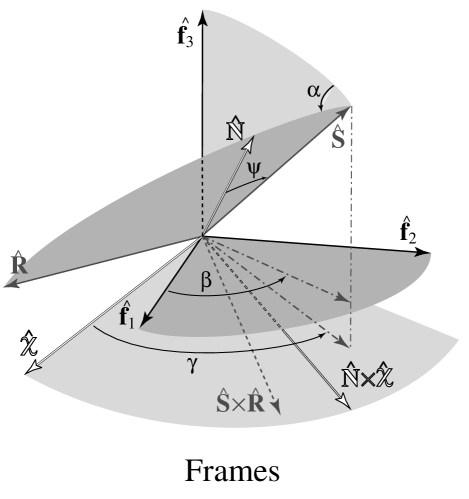
FIG. 1.: Space frame (${\hat{f}}_{r}$), spin frame ($\hat{S}$, $\hat{R}$, $\hat{S}\times\hat{R}$) and dynamical body frame ($\hat{N}$, $\hat{\chi}$, $\hat{N}\times\hat{\chi}$) for $N\geq 3$ particles. $\psi$ - angle between $\hat{N}$ and $\hat{S}$. $\alpha$ - angle between the planes $\hat{S}$-${\hat{f}}_{3}$ and $\hat{S}$-$\hat{R}$. $\beta$ - angle between ${\hat{f}}_{1}$ and the projection of $\hat{S}$ onto the plane ${\hat{f}}_{1}$-${\hat{f}}_{2}$. $\gamma$ - angle between $\hat{\chi}$ and the projection of $\hat{S}$ onto the plane $\hat{\chi}$-$\hat{N}\times\hat{\chi}$.

Owing to the results of Appendix C, which allow to re-express $S_{qa}=|{\vec{S}}_{qa}|$, $S^{3}_{qa}$, $\beta_{a}=tg^{-1}{{S^{2}_{qa}}\over{S^{1}_{qa}}}$ in terms of the final variables and owing to Eqs.(219), (254) which allow to get $\alpha_{a}=-tg^{-1}{{({\hat{S}}_{qa}\times{\hat{R}}_{a})^{3}}\over{({\hat{S}}_{qa}\times({\hat{S}}_{qa}\times{\hat{R}}_{a}))^{3}}}$, we can reconstruct the inverse canonical transformation.

The existence of the spin frame and of the dynamical body frame allows to define two decompositions of the relative variables, which make explicit the inverse canonical transformation. For the relative coordinates we get from Eqs. (219) and (C35)

$${\vec{\rho}}_{qa} = \rho_{qa}{\hat{R}}_{a}=\rho_{qa}[\vec{N}+(-)^{a+1}\vec{\chi}]=\rho_{qa}[|\vec{N}|\hat{N}+(-)^{a+1}\sqrt{1-{\vec{N}}^{2}}\hat{\chi}]=$$ (274)

$$= [{\vec{\rho}}_{qa}\cdot{\hat{S}}_{q}]{\hat{S}}_{q}+[{\vec{\rho}}_{qa}\cdot\hat{R}]\hat{R}+[{\vec{\rho}}_{qa}\cdot{\hat{S}}_{q}\times\hat{R}]{\hat{S}}_{q}\times\hat{R}=$$ (275)

$$= {{\rho_{qa}}\over{S_{q}}}\Big{[}\Big{(}|\vec{N}|\,{\check{S}}^{3}_{q}+(-)^{a+1}\sqrt{1-{\vec{N}}^{2}}\,{\check{S}}^{1}_{q}\Big{)}{\hat{S}}_{q}+$$ (276)

$$+ \Big{(}|\vec{N}|\sqrt{(S_{q})^{2}-({\check{S}}^{3}_{q})^{2}}-(-)^{a+1}\sqrt{1-{\vec{N}}^{2}}{{{\check{S}}^{1}_{q}{\check{S}}^{3}_{q}}\over{\sqrt{(S_{q})^{2}-({\check{S}}^{3}_{q})^{2}}}}\Big{)}\hat{R}-$$ (277)

$$- (-)^{a+1}\sqrt{1-{\vec{N}}^{2}}{{{\check{S}}^{2}_{q}}\over{\sqrt{(S_{q})^{2}-({\check{S}}^{3}_{q})^{2}}}}{\hat{S}}_{q}\times\hat{R}\Big{]}=$$ (278)

$$= {\vec{\rho}}_{qa}[S_{q},\alpha;S^{3}_{q},\beta;{\check{S}}^{3}_{q},\gamma;\rho_{qa},|\vec{N}|].$$ (279)

The analogous formulae for the relative momenta are [see Eq.(C47) for the expression of the body frame components of ${\vec{\pi}}_{qa}$]

$${\vec{\pi}}_{qa} = {\tilde{\pi}}_{qa}{\hat{R}}_{a}+{{S_{qa}}\over{\rho_{qa}}}{\hat{S}}_{qa}\times{\hat{R}}_{a}={\tilde{\pi}}_{qa}{\hat{\rho}}_{qa}+{{S_{qa}}\over{\rho_{qa}}}{\hat{S}}_{qa}\times{\hat{\rho}}_{a}=$$ (280)

$$= [{\vec{\pi}}_{qa}\cdot\hat{N}]\hat{N}+[{\vec{\pi}}_{qa}\cdot\hat{\chi}]\hat{\chi}+[{\vec{\pi}}_{qa}\cdot\hat{N}\times\hat{\chi}]\hat{N}\times\hat{\chi}=$$ (281)

$$= [{\vec{\pi}}_{qa}\cdot{\hat{S}}_{q}]{\hat{S}}_{q}+[{\vec{\pi}}_{qa}\cdot\hat{R}]\hat{R}+[{\vec{\pi}}_{qa}\cdot{\hat{S}}_{q}\times\hat{R}]{\hat{S}}_{q}\times\hat{R}=$$ (283)

$$= {1\over{S_{q}}}\Big{[}\Big{(}({\vec{\pi}}_{qa}\cdot\hat{N}){\check{S}}^{3}_{q}+({\vec{\pi}}_{qa}\cdot\hat{\chi}){\check{S}}^{1}_{q}+({\vec{\pi}}_{qa}\cdot\hat{N}\times\hat{\chi}){\check{S}}^{2}_{q}\Big{)}{\hat{S}}_{q}+$$ (284)

$$+ \Big{(}({\vec{\pi}}_{qa}\cdot\hat{N})\sqrt{(S_{q})^{2}-({\check{S}}^{3}_{q})^{2}}-[({\vec{\pi}}_{qa}\cdot\hat{\chi}+({\vec{\pi}}_{qa}\cdot\hat{N}\times\hat{\chi})]{{{\check{S}}^{1}_{q}{\check{S}}^{3}_{q}}\over{\sqrt{(S_{q})^{2}-({\check{S}}^{3}_{q})^{2}}}}\Big{)}\hat{R}+$$ (285)

$$+ [({\vec{\pi}}_{qa}\cdot\hat{\chi})-({\vec{\pi}}_{qa}\cdot\hat{N}\times\hat{\chi})]{{{\check{S}}^{2}_{q}{\check{S}}^{3}_{q}}\over{\sqrt{(S_{q})^{2}-({\check{S}}^{3}_{q})^{2}}}}\hat{R}\times{\hat{S}}_{q}\Big{]}=$$ (286)

$$= {\vec{\pi}}_{qa}[S_{q},\alpha;S^{3}_{q},\beta;{\check{S}}^{3}_{q},\gamma;|\vec{N}|,\xi;\rho_{qa},{\tilde{\pi}}_{qa}].$$ (287)

Finally, the results of Appendix D allow to perform a sequence of a canonical transformation to Euler angles $\tilde{\alpha}$, $\tilde{\beta}$, $\tilde{\gamma}$ with their conjugate momenta, followed by a transition to the anholonomic basis used in the orientation-shape bundle approach[9]

$$\begin{minipage}[t]{85.35826pt} \begin{tabular}[]{|lll|}\hline\cr$\alpha$&$\beta$&$\gamma$\\ \hline\cr$S_{q}={\check{S}}_{q}$&$S^{3}_{q}$&${\check{S}}_{q}^{3}$\\ \hline\cr\end{tabular} \end{minipage}\ {\longrightarrow\hskip 5.69046pt}\ \begin{minipage}[t]{85.35826pt} \begin{tabular}[]{|lll|}\hline\cr$\tilde{\alpha}$&$\tilde{\beta}$&$\tilde{\gamma}$\\ \hline\cr$p_{\tilde{\alpha}}$&$p_{\tilde{\beta}}$&$p_{\tilde{\gamma}}$\\ \hline\cr\end{tabular} \end{minipage}\ {{\buildrel{non\,\,can.}\over{\longrightarrow}}\hskip 5.69046pt}\ \begin{minipage}[b]{85.35826pt} \begin{tabular}[]{|lll|}\hline\cr$\tilde{\alpha}$&$\tilde{\beta}$&$\tilde{\gamma}$\\ \hline\cr${\check{S}}^{1}_{q}$&${\check{S}}^{2}_{q}$&${\check{S}}^{3}_{q}$\\ \hline\cr\end{tabular} \end{minipage}$$ (294)

$$S_{q} = {\check{S}}_{q}=\sqrt{({\check{S}}^{1}_{q})^{2}+({\check{S}}^{2}_{q})^{2}+({\check{S}}^{3}_{q})^{2}},$$ (296)

$$S^{3}_{q} = -sin\,\tilde{\beta}cos\,\tilde{\gamma}{\check{S}}^{1}_{q}+sin\,\tilde{\beta}sin\,\tilde{\gamma}{\check{S}}^{2}_{q}+cos\,\tilde{\beta}{\check{S}}^{3}_{q},$$ (297)

$$\alpha = arctg\,{{p_{\tilde{\beta}}tg\,\tilde{\beta}}\over{{\check{S}}_{q}-{{p_{\tilde{\alpha}}p_{\tilde{\gamma}}}\over{{\check{S}}_{q}cos\,\tilde{\beta}}}}},$$ (298)

$$\gamma = {{\pi}\over 2}-\tilde{\gamma}-arctg\,{{ctg\,\tilde{\beta}p_{\tilde{\gamma}}-{{p_{\tilde{\alpha}}}\over{sin\,\tilde{\beta}}}}\over{p_{\tilde{\beta}}}},$$ (299)

$$\beta = \tilde{\alpha}+arctg\,{{ctg\,\tilde{\beta}p_{\tilde{\alpha}}-{{p_{\tilde{\gamma}}}\over{sin\,\tilde{\beta}}}}\over{p_{\tilde{\beta}}}}-{{\pi}\over 2},$$ (300)

Here $p_{\tilde{\alpha}}$, $p_{\tilde{\beta}}$, $p_{\tilde{\gamma}}$ are the functions of $\tilde{\alpha}$, $\tilde{\beta}$, $\tilde{\gamma}$, ${\check{S}}^{r}_{q}$ given in Eqs.(D35). The equations (D35), (300), (219) and ${\check{S}}^{2}_{q}={\vec{S}}_{q}\cdot\hat{N}\times\hat{\chi}$ lead to the determination of the dynamical orientation variables $\tilde{\alpha}$, $\tilde{\beta}$, $\tilde{\gamma}$ in terms of ${\vec{\rho}}_{qa}$, ${\vec{\pi}}_{qa}$. Let us stress that, while in the orientation-shape bundle approach the orientation variables $\theta^{\alpha}$ are gauge variables, the Euler angles $\tilde{\alpha}$, $\tilde{\beta}$, $\tilde{\gamma}$ are uniquely determined in terms of the original configurations and momenta.

In conclusion, the complete transition to the anholonomic basis used in the static theory of the orientation-shape bundle is

$$\begin{minipage}[t]{142.26378pt} \begin{tabular}[]{|lll|l|l|}\hline\cr$\alpha$&$\beta$&$\gamma$&$|\vec{N}|$&$\rho_{qa}$\\ \hline\cr$S_{q}={\check{S}}_{q}$&$S^{3}_{q}$&${\check{S}}_{q}^{3}$&$\xi$&${\tilde{\pi}}_{qa}$\\ \hline\cr\end{tabular} \end{minipage}\ {{\buildrel{non\,\,can.}\over{\longrightarrow}}\hskip 5.69046pt}\ \begin{minipage}[b]{142.26378pt} \begin{tabular}[]{|lll|l|l|}\hline\cr$\tilde{\alpha}$&$\tilde{\beta}$&$\tilde{\gamma}$&$|\vec{N}|$&$\rho_{qa}$\\ \hline\cr${\check{S}}^{1}_{q}$&${\check{S}}^{2}_{q}$&${\check{S}}^{3}_{q}$&$\xi$&${\tilde{\pi}}_{qa}$\\ \hline\cr\end{tabular} \end{minipage}.$$ (301)

In order to further the comparison with the orientation-shape bundle approach, let us note the following relation between the space and body components of the relative coordinates. Eqs.(287), (301), (273) and (D24) imply

$$\rho^{r}_{qa} = {\cal R}^{r}{}_{s}(\tilde{\alpha},\tilde{\beta},\tilde{\gamma}){\check{\rho}}^{s}_{qa}(q),\quad\quad with$$ (306)

$${\check{\rho}}^{1}_{qa}(q)=(-)^{a+1}\rho_{qa}\sqrt{1-{\vec{N}}^{2}},\quad\quad{\check{\rho}}^{2}_{qa}(q)=0,\quad\quad{\check{\rho}}^{3}_{qa}(q)=\rho_{qa}|\vec{N}|,$$

$$and$$

$$S^{r}_{q} = {\cal R}^{r}{}_{s}(\tilde{\alpha},\tilde{\beta},\tilde{\gamma}){\check{S}}^{s}_{q},$$ (307)

so that the final visualization of our sequence of transformations is

$$\begin{minipage}[t]{142.26378pt} \begin{tabular}[]{|l|}\hline\cr${\vec{\rho}}_{qa}$\\ \hline\cr${\vec{\pi}}_{qa}$\\ \hline\cr\end{tabular} \end{minipage}\ {{\buildrel{non\,\,can.}\over{\longrightarrow}}\hskip 5.69046pt}\ \begin{minipage}[b]{142.26378pt} \begin{tabular}[]{|lll|l|}\hline\cr$\tilde{\alpha}$&$\tilde{\beta}$&$\tilde{\gamma}$&$q^{\mu}({\vec{\rho}}_{qa})$\\ \hline\cr${\check{S}}^{1}_{q}$&${\check{S}}^{2}_{q}$&${\check{S}}^{3}_{q}$&$p_{\mu}({\vec{\rho}}_{qa},{\vec{\pi}}_{qa})$\\ \hline\cr\end{tabular} \end{minipage}.$$ (308)

Note furthermore that we get ${\check{\rho}}^{2}_{qa}={\vec{\rho}}_{qa}\cdot\hat{N}\times\hat{\chi}=0$ by construction and this entails that using our dynamical body frame is equivalent to a convention (xxzz gauge) about the body frame of the type of xxz and similar gauges quoted in Ref.[9] .

Finally, we can give the expression of the Hamiltonian for relative motions in terms of the anholonomic Darboux basis of Eqs.(300). By using Eq.(C84) we get

$$H_{rel} = {1\over{2{\vec{N}}^{2}}}\Big{[}{1\over 2}({{k^{-1}{}_{11}}\over{\rho^{2}_{q1}}}+{{k^{-1}{}_{22}}\over{\rho^{2}_{q2}}})+{{k^{-1}{}_{12}}\over{\rho_{q1}\rho_{q2}}}\Big{]}({\check{S}}^{1}_{q})^{2}+$$ (309)

$$+ {1\over 2}\Big{[}{1\over 2}({{k^{-1}{}_{11}}\over{\rho^{2}_{q1}}}+{{k^{-1}{}_{22}}\over{\rho^{2}_{q2}}})+{{k^{-1}{}_{12}(2{\vec{N}}^{2}-1)}\over{\rho_{q1}\rho_{q2}}}\Big{]}({\check{S}}^{2}_{q})^{2}+$$ (310)

$$+ {1\over{2(1-{\vec{N}}^{2})}}\Big{[}{1\over 2}({{k^{-1}{}_{11}}\over{\rho^{2}_{q1}}}+{{k^{-1}{}_{22}}\over{\rho^{2}_{q2}}})-{{k^{-1}{}_{12}}\over{\rho_{q1}\rho_{q2}}}\Big{]}({\check{S}}^{3}_{q})^{2}+$$ (311)

$$+ \sqrt{1-{\vec{N}}^{2}}\Big{[}{{\xi}\over 2}({{k^{-1}{}_{11}}\over{\rho^{2}_{q1}}}-{{k^{-1}{}_{22}}\over{\rho^{2}_{q2}}})+2k^{-1}{}_{12}|\vec{N}|\sqrt{1-{\vec{N}}^{2}}({{{\tilde{\pi}}_{q1}}\over{\rho_{q2}}}-{{{\tilde{\pi}}_{q2}}\over{\rho_{q1}}})\Big{]}{\check{S}}_{q}^{2}-$$ (312)

$$- {1\over{2|\vec{N}|\sqrt{1-{\vec{N}}^{2}}}}({{k^{-1}{}_{11}}\over{\rho^{2}_{q1}}}-{{k^{-1}{}_{22}}\over{\rho^{2}_{q2}}}){\check{S}}^{1}_{q}{\check{S}}^{3}_{q}+$$ (313)

$$+ k^{-1}{}_{11}\Big{[}{\tilde{\pi}}^{2}_{q1}+{{\xi^{2}(1-{\vec{N}}^{2})}\over{4\rho^{2}_{q1}}}\Big{]}+k^{-1}{}_{22}\Big{[}{\tilde{\pi}}^{2}_{q2}+{{\xi^{2}(1-{\vec{N}}^{2})}\over{4\rho^{2}_{q2}}}\Big{]}+$$ (314)

$$+ 2k^{-1}{}_{12}\Big{[}(2{\vec{N}}^{2}-1){\tilde{\pi}}_{q1}{\tilde{\pi}}_{q2}-|\vec{N}|(1-{\vec{N}}^{2})\xi({{{\tilde{\pi}}_{q1}}\over{\rho_{q2}}}+{{{\tilde{\pi}}_{q2}}\over{\rho_{q1}}})+$$ (315)

$$+ {{\xi^{2}(1-{\vec{N}}^{2})(2{\vec{N}}^{2}-1)}\over{4\rho_{q1}\rho_{q2}}}\Big{]}\,{\buildrel{def}\over{=}}$$ (316)

$${\buildrel{def}\over{=}}\, {1\over 2}\Big{[}{\check{S}}_{q}^{r}({\check{\cal I}}^{-1})^{rs}{\check{S}}_{q}^{s}+{\tilde{g}}^{\mu\nu}(p_{\mu}-{\vec{S}}_{q}\cdot{\vec{\cal A}}_{\mu})(p_{\nu}-{\check{\vec{S}}}_{q}\cdot{\check{\vec{\cal A}}}_{\nu})\Big{]}=$$ (317)

$$= {1\over 2}({\check{S}}_{q}^{r},\,p_{\mu})\left(\begin{array}[]{cc}({\check{\cal I}}^{-1})^{rs}+{\tilde{g}}^{\alpha\beta}{\check{\cal A}}^{r}_{\mu}{\check{\cal A}}^{s}_{\nu}&-{\tilde{g}}^{\nu\alpha}{\check{\cal A}}^{r}_{\alpha}\\ -{\tilde{g}}^{\mu\alpha}{\check{\cal A}}^{s}_{\alpha}&{\tilde{g}}^{\mu\nu}\end{array}\right)\left(\begin{array}[]{c}{\check{S}}_{q}^{s}\\ p_{\nu}\end{array}\right).$$ (322)

where $q^{\mu}=(\rho_{q1},\rho_{q2},|\vec{N}|)$, $p_{\mu}=({\tilde{\pi}}_{q1},{\tilde{\pi}}_{q2},\xi)$ are the dynamical shape variables. In the last two lines we have rewritten the Hamiltonian in the form of Eq.(B63).

In Appendix E we evaluate the quantities ${\check{\cal A}}^{r}_{\mu}(q)$, ${\tilde{g}}^{\mu\nu}(q)$, ${\check{\cal I}}^{-1rs}(q)$ appearing in the standard static theory of the orientation-shape bundle in the xxzz gauge, adopting the convention induced by the dynamical body frame. Recall that the special xxzz gauge potentials ${\check{\cal A}}^{r}_{\mu}(q)$ are measurable quantities in our approach. The same holds for the angular velocity in the evolving dynamical body frame.

In the static orientation-shape trivial SO(3) principal bundle approach the Hamiltonian version of the conditions ${\check{S}}^{r}_{q}=0$ and ${\dot{q}}^{\mu}=0$, definitory of C-horizontality and verticality respectively, is given by Eq.(128). Note that the definition $({\check{S}}^{r}_{q},\,p_{\mu})_{v}=({\check{S}}^{r}_{q},\,p_{\mu}{|}_{\dot{q}=0}={\vec{S}}_{q}\cdot{\vec{\cal A}}_{\mu}(q))$ of vertical rotational motion ${\dot{q}}^{\mu}=0$ is still valid in our dynamical body frame approach. By using Eq.(E10) to find $p_{\mu}{|}_{\dot{q}=0}$, we recover the rotational kinetic energy (the centrifugal potential) $H^{(rot)}_{rel}={1\over 2}{\check{S}}_{q}^{r}({\check{\cal I}}^{-1})^{rs}{\check{S}}_{q}^{s}$ of the xxzz gauge.

On the other hand, the C-horizontal component should be determined by the condition ${\check{S}}^{r}_{q}=0$. Since our construction requires $S_{q}\not=0$, we cannot utilize it. In our approach the measurable vibrational kinetic energy $H^{(vib)}_{rel}$ for ${\vec{S}}\not=0$ non-singular N=3 configurations is obtained by restricting ${\check{S}}^{r}_{q}$ in $H_{rel}$ to the value ${\check{S}}^{r}_{q}{|}_{{\check{\omega}}^{s}=0}$ of Eq.(E38), upon the requirement that the dynamical angular velocity vanishes in the xxzz gauge. From Eq.(E38) we get

$${\check{S}}^{1}_{q}{|}_{{\check{\omega}}^{r}=0}={\check{S}}^{3}_{q}{|}_{{\check{\omega}}^{r}=0}=0,$$ (326)

$${\check{S}}^{2}_{q}{|}_{{\check{\omega}}^{r}=0}=-{{\sqrt{1-{\vec{N}}^{2}}\Big{[}{{\xi}\over 2}\Big{(}{{k^{-1}_{11}}\over{\rho_{q1}^{2}}}-{{k^{-1}_{22}}\over{\rho_{q2}^{2}}}\Big{)}+2k^{-1}_{12}|\vec{N}|\sqrt{1-{\vec{N}}^{2}}\Big{(}{{{\tilde{\pi}}_{q1}}\over{\rho_{q2}}}-{{{\tilde{\pi}}_{q2}}\over{\rho_{q1}}}\Big{)}\Big{]}}\over{{1\over 2}\Big{(}{{k^{-1}_{11}}\over{\rho_{q1}^{2}}}+{{k^{-1}_{22}}\over{\rho_{q2}^{2}}}\Big{)}+{{k^{-1}_{12}(2{\vec{N}}^{2}-1)}\over{\rho_{q1}\rho_{q2}}}}},$$

$$\Downarrow$$

$$H_{rel} {|}_{{\check{\omega}}^{r}=0}=k^{-1}_{11}\Big{[}{\tilde{\pi}}^{2}_{q1}+{{\xi^{2}(1-{\vec{N}}^{2})}\over{4\rho_{q1}^{2}}}\Big{]}+k^{-1}_{22}\Big{[}{\tilde{\pi}}^{2}_{q2}+{{\xi^{2}(1-{\vec{N}}^{2})}\over{4\rho_{q2}^{2}}}\Big{]}+$$ (330)

$$+2k^{-1}_{12}\Big{[}(2{\vec{N}}^{2}-1){\tilde{\pi}}_{q1}{\tilde{\pi}}_{q2}-|\vec{N}|(1-{\vec{N}}^{2})\xi\Big{(}{{{\tilde{\pi}}_{q1}}\over{\rho_{q2}}}+{{{\tilde{\pi}}_{q2}}\over{\rho_{q1}}}\Big{)}+{{\xi^{2}(1-{\vec{N}}^{2})(2{\vec{N}}^{2}-1)}\over{4\rho_{q1}\rho_{q2}}}\Big{]}-$$

$$-{1\over 2}{{(1-{\vec{N}}^{2})\Big{[}{{\xi}\over 2}\Big{(}{{k^{-1}_{11}}\over{\rho_{q1}^{2}}}-{{k^{-1}_{22}}\over{\rho_{q2}^{2}}}\Big{)}+2k^{-1}_{12}|\vec{N}|\sqrt{1-{\vec{N}}^{2}}\Big{(}{{{\tilde{\pi}}_{q1}}\over{\rho_{q2}}}-{{{\tilde{\pi}}_{q2}}\over{\rho_{q1}}}\Big{)}\Big{]}}\over{{1\over 2}\Big{(}{{k^{-1}_{11}}\over{\rho_{q1}^{2}}}+{{k^{-1}_{22}}\over{\rho_{q2}^{2}}}\Big{)}+{{k^{-1}_{12}(2{\vec{N}}^{2}-1)}\over{\rho_{q1}\rho_{q2}}}}}.$$

Let us remark that with this definition we get $H_{rel}\not=H^{(rot)}_{rel}+H^{(vib)}_{rel}$, differently from the static orientation-shape bundle result associated with the C-connection . In order to get the theory with the Jacobi normal coordinates one has to perform our sequence of canonical transformations after having diagonalized $k_{ab}$.

Let us end this Subsection by recalling that in Ref.[10] the N=3 shape space is parametrized with the following configurational coordinate system $(w,w_{1},w_{2})$: $w=\rho_{q1}^{2}+\rho_{q2}^{2}$ ($\sqrt{w}$ is the hyperradius), $w_{1}=\rho_{q1}^{2}-\rho_{q2}^{2}$, $w_{2}=2{\vec{\rho}}_{q1}\cdot{\vec{\rho}}_{q2}$ with the physical region of non-singular configurations defined by $\sqrt{w_{1}^{2}+w_{2}^{2}}\leq w\leq\infty$, $-\infty\leq w_{1},w_{2}\leq\infty$. The variable $w$ may be replaced by $w_{3}=2|{\vec{\rho}}_{q1}\times{\vec{\rho}}_{q2}|\geq 0$ ($w_{3}\geq 0$ is the physical region), because $w^{2}=w^{2}_{1}+w_{2}^{2}+w_{3}^{2}$. Thus, another basis for the N=3 shape space is $(w_{1},w_{2},w_{3})$. A further basis $(w,\chi,\psi)$ is obtained by putting $w_{1}=wcos\,\chi cos\,\psi$, $w_{1}=wcos\,\chi sin\,\psi$, $w_{2}=wsin\,\chi$, ($\chi,\psi$ hyperspherical angles), The quantities $w$ and $a=w_{1}^{2}+w_{2}^{2}=(\rho_{q1}^{2}-\rho_{q2}^{2})^{2}+4({\vec{\rho}}_{q1}\cdot{\vec{\rho}}_{q2})^{2}$ [$w_{3}=\sqrt{w^{2}-a}$] are democratic invariants, and still another basis is $(w,w_{3},\alpha)$, with $\alpha$ the angle parametrizing the democracy group SO(2). In our spin basis we have the 3 purely configurational shape variables $\rho_{q1}$, $\rho_{q2}$ and $|\vec{N}|=\sqrt{{{1+{\hat{\rho}}_{q1}\cdot{\hat{\rho}}_{q2}}\over 2}}$. We can define a point canonical transformation to $w=\rho_{q1}^{2}+\rho_{q2}^{2}$, $w_{1}=\rho_{q1}^{2}-\rho_{q2}^{2}$, $w_{2}=2\rho_{q1}\rho_{q2}(2{\vec{N}}^{2}-1)$, and then find the corresponding momenta.

C N-Body Systems.

Let us now consider the general case with $N\geq 4$ without introducing Jacobi normal coordinates. Instead of coupling the centers of mass of particle clusters as it is done with Jacobi coordinates (center-of-mass clusters), the canonical spin bases will be obtained by coupling the spins of the 2-body subsystems (relative particles) ${\vec{\rho}}_{qa}$, ${\vec{\pi}}_{qa}$, $a=1,..,N-1$, defined in Eqs.(17), in all possible ways (spin clusters from the addition of angular momenta). Let us stress that we can build a spin basis with a pattern of spin clusters completely unrelated to a possible pre-existing center-of-mass clustering.

Let us consider the case $N=4$ as a prototype of the general construction. We have now three relative variables ${\vec{\rho}}_{q1}$, ${\vec{\rho}}_{q2}$, ${\vec{\rho}}_{q3}$ and related momenta ${\vec{\pi}}_{q1}$, ${\vec{\pi}}_{q2}$, ${\vec{\pi}}_{q3}$. In the following formulas we use the convention that the subscripts $a,b,c$ mean any permutation of $1,2,3$.

By using the explicit construction given in Appendix F, we define the following sequence of canonical transformations (we assume $S_{q}\not=0$; $S_{qA}\not=0$, $A=a,b,c$) corresponding to the spin clustering pattern $abc\mapsto(ab)c\mapsto((ab)c)$ [build first the spin cluster $(ab)$, then the spin cluster $((ab)c)$]:

$$\begin{minipage}[t]{85.35826pt} \begin{tabular}[]{|lll|}\hline\cr${\vec{\rho}}_{qa}$&${\vec{\rho}}_{qb}$&${\vec{\rho}}_{qc}$\\ ${\vec{\pi}}_{qa}$&${\vec{\pi}}_{qb}$&${\vec{\pi}}_{qc}$\\ \hline\cr\end{tabular} \end{minipage}\ {\longrightarrow\hskip 5.69046pt}\$$ (333)

$$\ {\longrightarrow\hskip 5.69046pt}\ \begin{minipage}[t]{199.16928pt} \begin{tabular}[]{|ll|ll|ll|lll|}\hline\cr$\alpha_{a}$&$\beta_{a}$&$\alpha_{b}$&$\beta_{b}$&$\alpha_{c}$&$\beta_{c}$&$\rho_{qa}$&$\rho_{qb}$&$\rho_{qc}$\\ \hline\cr$S_{qa}$&$S^{3}_{qa}$&$S_{qb}$&$S^{3}_{qb}$&$S_{qc}$&$S^{3}_{qc}$&${\tilde{\pi}}_{qa}$&${\tilde{\pi}}_{qb}$&${\tilde{\pi}}_{qc}$\\ \hline\cr\end{tabular} \end{minipage}\ {\longrightarrow\hskip 5.69046pt}\$$ (336)

$$\ {{\buildrel{(ab)c}\over{\longrightarrow}}\hskip 5.69046pt}\ \begin{minipage}[t]{341.43306pt} \begin{tabular}[]{|ccc|cc|cccc|}\hline\cr$\alpha_{(ab)}$&$\beta_{(ab)}$&$\gamma_{(ab)}$&$\alpha_{c}$&$\beta_{c}$&$|{\vec{N}}_{(ab)}|$&$\rho_{qa}$&$\rho_{qb}$&$\rho_{qc}$\\ \hline\cr$S_{q(ab)}$&$S^{3}_{q(ab)}$&${\check{S}}_{q(ab)}^{3}={\vec{S}}_{q(ab)}\cdot{\hat{N}}_{(ab)}$&$S_{qc}$&$S^{3}_{qc}$&$\xi_{(ab)}$&${\tilde{\pi}}_{qa}$&${\tilde{\pi}}_{qb}$&${\tilde{\pi}}_{qc}$\\ \hline\cr\end{tabular} \end{minipage}\ {\longrightarrow\hskip 5.69046pt}\$$ (339)

$$\ {\longrightarrow\hskip 5.69046pt}\ \begin{minipage}[t]{369.88582pt} \begin{tabular}[]{|ccc|cccccc|}\hline\cr$\alpha_{((ab)c)}$&$\beta_{((ab)c)}$&$\gamma_{((ab)c)}$&$|{\vec{N}}_{((ab)c)}|$&$\gamma_{(ab)}$&$|{\vec{N}}_{(ab)}|$&$\rho_{qa}$&$\rho_{qb}$&$\rho_{qc}$\\ \hline\cr$S_{q}={\check{S}}_{q}$&$S^{3}_{q}$&${\check{S}}_{q}^{3}={\vec{S}}_{q}\cdot{\hat{N}}_{((ab)c)}$&$\xi_{((ab)c)}$&${\vec{S}}_{q(ab)}\cdot{\hat{N}}_{(ab)}$&$\xi_{(ab)}$&${\tilde{\pi}}_{qa}$&${\tilde{\pi}}_{qb}$&${\tilde{\pi}}_{qc}$\\ \hline\cr\end{tabular} \end{minipage}\ {\rightarrow\hskip 5.69046pt}\$$ (342)

$$\ {{\buildrel{non\,can.}\over{\longrightarrow}}\hskip 5.69046pt}\ \begin{minipage}[t]{341.43306pt} \begin{tabular}[]{|ccc|cccccc|}\hline\cr$\tilde{\alpha}$&$\tilde{\beta}$&$\tilde{\gamma}$&$|{\vec{N}}_{((ab)c)}|$&$\gamma_{(ab)}$&$|{\vec{N}}_{(ab)}|$&$\rho_{qa}$&$\rho_{qb}$&$\rho_{qc}$\\ \hline\cr${\check{S}}_{q}^{1}$&${\check{S}}^{2}_{q}$&${\check{S}}_{q}^{3}$&$\xi_{((ab)c)}$&$\Omega_{(ab)}={\vec{S}}_{q(ab)}\cdot{\hat{N}}_{(ab)}$&$\xi_{(ab)}$&${\tilde{\pi}}_{qa}$&${\tilde{\pi}}_{qb}$&${\tilde{\pi}}_{qc}$\\ \hline\cr\end{tabular} \end{minipage}.$$ (345)

The first non-point canonical transformation is based on the existence of the three unit vectors ${\hat{R}}_{A}$, $A=a,b,c$, and of three E(3) realizations with generators ${\vec{S}}_{qA}$, ${\hat{R}}_{A}$ and fixed values (${\hat{R}}_{A}^{2}=1$, ${\vec{S}}_{A}\cdot{\hat{R}}_{A}=0$) of the invariants. Use Eqs.(205), (208) and (211).

In the next canonical transformation the spins of the relative particles $a$ and $b$ are coupled to form the spin cluster $(ab)$, leaving the relative particle $c$ as a spectator. We use Eq.(219) to define ${\vec{N}}_{(ab)}={1\over 2}({\hat{R}}_{a}+{\hat{R}}_{b})$, ${\vec{\chi}}_{(ab)}={1\over 2}({\hat{R}}_{a}-{\hat{R}}_{b})$, ${\vec{S}}_{(ab)}={\vec{S}}_{qa}+{\vec{S}}_{qb}$, ${\vec{W}}_{q(ab)}={\vec{S}}_{qa}-{\vec{S}}_{qb}$. We get ${\vec{N}}_{(ab)}\cdot{\vec{\chi}}_{(ab)}=0$, $\{N^{r}_{(ab)},N^{s}_{(ab)}\}=\{N^{r}_{(ab)},\chi^{s}_{(ab)}\}=\{\chi^{r}_{(ab)},\chi^{s}_{(ab)}\}=0$ and a new E(3) realization generated by ${\vec{S}}_{(ab)}$ and ${\vec{N}}_{(ab)}$, with non-fixed invariants $|{\vec{N}}_{(ab)}|$, ${\vec{S}}_{(ab)}\cdot{\hat{N}}_{(ab)}\,{\buildrel{def}\over{=}}\,\Omega_{(ab)}$. From Eqs.(287) it follows

$${\vec{\rho}}_{qa}=\rho_{qa}\Big{[}|{\vec{N}}_{(ab)}|{\hat{N}}_{(ab)}+\sqrt{1-{\vec{N}}^{2}_{(ab)}}{\hat{\chi}}_{(ab)}\Big{]},$$ (347)

$${\vec{\rho}}_{qb}=\rho_{qb}\Big{[}|{\vec{N}}_{(ab)}|{\hat{N}}_{(ab)}-\sqrt{1-{\vec{N}}^{2}_{(ab)}}{\hat{\chi}}_{(ab)}\Big{]},$$ (348)

$${\vec{\rho}}_{qc}=\rho_{qc}{\hat{R}}_{c}.$$ (349)

Eq.(240) defines $\alpha_{(ab)}$ and $\beta_{(ab)}$, so that Eq.(253) defines a unit vector ${\hat{R}}_{(ab)}$ with ${\vec{S}}_{(ab)}\cdot{\hat{R}}_{(ab)}=0$, $\{{\hat{R}}^{r}_{(ab)},{\hat{R}}^{s}_{(ab)}\}=0$. This unit vector identifies the spin cluster $(ab)$ in the same way as the unit vectors ${\hat{R}}_{A}={\hat{\vec{\rho}}}_{qA}$ identify the relative particles $A$.

The next step is the coupling of the spin cluster $(ab)$ with unit vector ${\hat{R}}_{(ab)}$ [described by the canonical variables $\alpha_{(ab)}$, $S_{(ab)}$, $\beta_{(ab)}$ $S^{3}_{(ab)}$] with the relative particle $c$ with unit vector ${\hat{R}}_{c}$ and described by $\alpha_{c}$, $S_{qc}$, $\beta_{c}$, $S^{3}_{qc}$: this builds the spin cluster $((ab)c)$.

Again, Eq.(219) allows to define ${\vec{N}}_{((ab)c)}={1\over 2}({\hat{R}}_{(ab)}+{\hat{R}}_{c})$, ${\vec{\chi}}_{((ab)c)}={1\over 2}({\hat{R}}_{(ab)}-{\hat{R}}_{c})$, ${\vec{S}}_{q}={\vec{S}}_{q((ab)c)}={\vec{S}}_{q(ab)}+{\vec{S}}_{qc}$, ${\vec{W}}_{q((ab)c)}={\vec{S}}_{q(ab)}-{\vec{S}}_{qc}$. Since we have ${\vec{N}}_{((ab)c)}\cdot{\vec{\chi}}_{((ab)c)}=0$ and $\{N^{r}_{((ab)c)},N^{s}_{((ab)c)}\}=\{N^{r}_{((ab)c)},\chi^{s}_{((ab)c)}\}=\{\chi^{r}_{((ab)c)},\chi^{s}_{((ab)c)}\}=0$ due to $\{{\hat{R}}^{r}_{(ab)},{\hat{R}}_{c}^{s}\}=0$, a new E(3) realization generated by ${\vec{S}}_{q}$ and ${\vec{N}}_{((ab)c)}$ with non-fixed invariants $|{\vec{N}}_{((ab)c)}|$, ${\vec{S}}_{q}\cdot{\hat{N}}_{((ab)c)}={\check{S}}^{3}_{q}$ emerges. Eq.(240) defines $\alpha_{((ab)c)}$ and $\beta_{((ab)c)}$, so that Eq.(253) allows to identify a final unit vector ${\hat{R}}_{((ab)c)}$ with ${\vec{S}}_{q}\cdot{\hat{R}}_{((ab)c)}=0$ and $\{{\hat{R}}_{((ab)c)}^{r},{\hat{R}}^{s}_{((ab)c)}\}=0$.

In conclusion, when $S_{q}\not=0$, we find both a spin frame ${\hat{S}}_{q}$, ${\hat{R}}_{((ab)c)}$, ${\hat{R}}_{((ab)c)}\times{\hat{S}}_{q}$ and a dynamical body frame ${\hat{\chi}}_{((ab)c)}$, ${\hat{N}}_{((ab)c)}\times{\hat{\chi}}_{((ab)c)}$, ${\hat{N}}_{((ab)c)}$, like in the 3-body case. There is an important difference, however: the orthonormal vectors ${\vec{N}}_{((ab)c)}$ and ${\vec{\chi}}_{((ab)c)}$ depend on the momenta of the relative particles $a$ and $b$ through ${\hat{R}}_{(ab)}$, so that our results do not share any relation with the N=4 non-trivial SO(3) principal bundle of the orientation-shape bundle approach.

The final 6 dynamical shape variables are $q^{\mu}=\{|{\vec{N}}_{((ab)c)}|,\gamma_{(ab)},|{\vec{N}}_{(ab)}|,\rho_{qa},\rho_{qb},\rho_{qc}\}$. While the last four depend only on the original relative coordinates ${\vec{\rho}}_{qA}$, $A=a,b,c$, the first two depend also on the original momenta ${\vec{\pi}}_{qA}$: therefore they are generalized shape variables. By using Appendix D, we obtain

$$\rho^{r}_{qA}={\cal R}^{rs}(\tilde{\alpha},\tilde{\beta},\tilde{\gamma})\,{\check{\rho}}^{s}_{qA}(q^{\mu},p_{\mu},{\check{S}}^{r}_{q}),\qquad A=a,b,c.$$ (350)

This means that for N=4 the dynamical body frame components ${\check{\rho}}^{r}_{qA}$ depend also on the dynamical shape momenta and on the dynamical body frame components of the spin. It is clear that this result stands completely outside the orientation-shape bundle approach.

As shown in Appendix F, starting from the Hamiltonian $H_{rel((ab)c)}$ expressed in the final variables, we can define a rotational Hamiltonian $H^{(rot)}_{rel((ab)c)}$ (for ${\dot{q}}^{\mu}=0$, see Eqs.(F164)) and a vibrational Hamiltonian $H^{(vib)}_{rel((ab)c)}$ (vanishing of the physical dynamical angular velocity ${\check{\omega}}^{r}_{((ab)c)}=0$, see Eqs.(F182)), but $H_{rel((ab)c)}$ fails to be the sum of these two Hamiltonians showing once again the non separability of rotations and vibrations. Let us stress that in the rotational Hamiltonian (F164) we find tan inertia-like tensor depending only on the dynamical shape variables. A similar result, however, does not hold for the spin-angular velocity relation (F175) due to the presence of the shape momenta $\xi_{(ab)}$ and $\xi_{((ab)c)}$.

The price to be paid for the existence of 3 global dynamical body frames for N=4 is a more complicated form of the Hamiltonian kinetic energy. On the other hand, dynamical vibrations and dynamical angular velocity are measurable quantities in each dynamical body frame.

For N=5 we can repeat the previous construction either with the sequence of spin clusterings $abcd\mapsto(ab)cd\mapsto((ab)c)d)\mapsto(((ab)c)d)$ or with the sequence $abcd\mapsto(ab)(cd)\mapsto((ab)(cd))$ [$a,b,c,d$ any permutation of 1,2,3,4] as said in the Introduction. Each spin cluster $(...)$ will be identified by the unit vector ${\hat{R}}_{(...)}$, axis of the spin frame of the cluster. All the final dynamical body frames built with this construction will have their axes depending on both the original configurations and momenta.

This construction is trivially generalized to any N: we have only to classify all the possible spin clustering patterns.

Therefore, for $N\geq 4$ our sequence of canonical and non-canonical transformations leads to the following result, to be compared with Eq.(301) of the 3-body case

Sˇ1qSˇ2qSˇ3qpμ(ρ→q​A,π→q​A).\begin{minipage}[t]{142.26378pt} \begin{tabular}[]{|l|}\hline\cr${\vec{\rho}}_{qA}$\\ \hline\cr${\vec{\pi}}_{qA}$\\ \hline\cr\end{tabular} \end{minipage}\ {{\buildrel{non\,\,can.}\over{\longrightarrow}}\hskip 5.69046pt}\ \begin{minipage}[b]{142.26378pt} \begin{tabular}[]{|lll|l|}\hline\cr$\tilde{\alpha}$&$\tilde{\beta}$&$\tilde{\gamma}$&$q^{\mu}({\vec{\rho}}_{qA},{\vec{\pi}}_{qA})$\\ \hline\cr${\check{S}}^{1}_{q}$&${\check{S}}^{2}_{q}$&${\check{S}}^{3}_{q}$&$p_{\mu}({\vec{\rho}}_{qA},{\vec{\pi}}_{qA}$)\\ \hline\cr\end{tabular} \end{minipage}.

~α~β~γqμ(→ρqA,→πqA) (351)

This state of affairs suggests that for $N\geq 4$ and with $S_{q}\not=0$, $S_{qA}\not=0$, $A=a,b,c$, namely when the standard (3N-3)-dimensional orientation-shape bundle is not trivial, the original (6N-6)-dimensional relative phase space admits the definition of as many dynamical body frames as spin canonical bases , which are globally defined (apart isolated coordinate singularities) for the non-singular N-body configurations with ${\vec{S}}_{q}\not=0$ (and with nonzero spin for each spin subcluster).

These dynamical body frames do not correspond to local cross sections of the static non-trivial orientation-shape SO(3) principal bundle and the spin canonical bases do not coincide with the canonical bases associated with the static theory. Therefore, we do not find gauge potentials as well as all the other quantities evaluated in Appendix E for N=3.

IV The Case of Interacting Particles.

Although we have defined the kinematics for free particles, the introduction of potentials is straightforward.

In the case N=2, the general form of a 2-body potential is $V({\vec{\rho}}_{q}^{2},{\vec{\rho}}_{q}\cdot{\vec{\pi}}_{q},{\vec{\pi}}^{2}_{q})=V(\rho^{2}_{q},\rho_{q}{\tilde{\pi}}_{q},{\tilde{\pi}}^{2}_{q}+{{S^{2}_{q}}\over{\rho^{2}_{q}}})$.

In the case N=3, suppose there is a potential $V({\vec{\eta}}_{ij}\cdot{\vec{\eta}}_{hk})$ with ${\vec{\eta}}_{ij}={\vec{\eta}}_{i}-{\vec{\eta}}_{j}$ . Then, since Eqs. (41) and (287) imply

$${\vec{\eta}}_{ij} = {1\over{\sqrt{3}}}\sum_{a=1}^{2}(\Gamma_{ai}-\Gamma_{aj}){\vec{\rho}}_{qa}={1\over{\sqrt{3}}}\sum_{a=1}^{2}(\Gamma_{ai}-\Gamma_{aj})\rho_{qa}[\vec{N}+(-)^{a+1}\vec{\chi}],$$ (352)

$${\vec{\eta}}_{ij}\cdot{\vec{\eta}}_{hk} = {1\over 3}\sum_{a,b}^{1,2}(\Gamma_{ai}-\Gamma_{aj})(\Gamma_{bh}-\Gamma_{bk})\rho_{qa}\rho_{qb}[{\vec{N}}^{2}+(-)^{a+b}(1-{\vec{N}}^{2})]=$$ (354)

$$= {1\over 3}\sum_{a=1}^{2}(\Gamma_{ai}-\Gamma_{aj})(\Gamma_{ah}-\Gamma_{ak})(\rho_{qa})^{2}+$$ (355)

$$+ {1\over 3}[(\Gamma_{1i}-\Gamma_{1j})(\Gamma_{2h}-\Gamma_{2k})+(\Gamma_{2i}-\Gamma_{2j})(\Gamma_{1h}-\Gamma_{1k})\rho_{q1}\rho_{q2}(2{\vec{N}}^{2}-1),$$ (356)

it turns out that the potential is a function of $\rho_{q1}^{2}$, $\rho_{q2}^{2}$, $(2{\vec{N}}^{2}-1)\rho_{q1}\rho_{q2}$. On the other hand, if the potential is $V({\vec{\eta}}_{ij}\cdot{\vec{\eta}}_{hk},{\vec{\kappa}}_{i}\cdot{\vec{\eta}}_{hk})$, Eqs.(287) and (C47) give the momentum dependence

$${\vec{\kappa}}_{i}\cdot{\vec{\eta}}_{hk} \approx \sum_{a,b}^{1,2}\gamma_{ai}(\Gamma_{bh}-\Gamma_{bk})\rho_{qb}\Big{(}{\tilde{\pi}}_{qa}[{\vec{N}}^{2}+(-)^{a+b+1}(1-{\vec{N}}^{2})]+$$ (357)

$$+ {{|\vec{N}|\sqrt{1-{\vec{N}}^{2}}}\over{2\rho_{qa}}}[(-)^{a}+(-)^{b+1}]({\check{S}}^{2}_{q}+(-)^{a+1}\xi\sqrt{1-{\vec{N}}^{2}})\Big{)}.$$ (358)

By means of the same equations it is possible to study a dependence upon ${\vec{\kappa}}_{i}\cdot{\vec{\kappa}}_{j}$.

For $N\geq 4$, even a potential of the form $V({\vec{\eta}}_{ij}\cdot{\vec{\eta}}_{hk}))$ with ${\vec{\eta}}_{ij}={\vec{\eta}}_{i}-{\vec{\eta}}_{j}$ turns out to be shape momentum dependent, since we have

$$V({\vec{\eta}}_{ij}\cdot{\vec{\eta}}_{hk})=V[{1\over N}\sum_{a,b}^{1,..,N-1}(\Gamma_{ai}-\Gamma_{aj})(\Gamma_{bh}-\Gamma_{bk}){\vec{\rho}}_{qa}\cdot{\vec{\rho}}_{qb}].$$ (359)

In particular, for N=4, due to Eq.(F70), in the pattern $((ab)c)$ we get $V={\tilde{V}}_{((ab)c)}[\rho_{qa},\rho_{qb},\rho_{qc},|{\vec{N}}_{((ab)c)}|,\gamma_{(ab)},|{\vec{N}}_{(ab)}|;\,\xi_{((ab)c)},\Omega_{(ab)};\,{\check{S}}^{r}_{q}]$.

For more general potentials $V({\vec{\eta}}_{ij}\cdot{\vec{\eta}}_{hk},{\vec{\kappa}}_{i}\cdot{\vec{\eta}}_{hk},{\vec{\kappa}}_{i}\cdot{\vec{\kappa}}_{j})$, like the non-relativistic limit of the relativistic Darwin potential of Ref.[13], more complicated expressions are obtained.

Finally, let us remark that both in the free and the interacting cases it is easier to solve the original Hamilton equations, rather than the equations for the orientation-shape coordinates, and then use the canonical transformation to find the time evolution of the dynamical body frame and related variables.

V Conclusions.

While it is possible to separate out absolute translations and relative motions in a global way, a global separation of absolute rotations from the associated notion of vibrations is not feasible because of the non-Abelian nature of rotations.

This fact gave origin to the orientation-shape SO(3) principal bundle approach described in Ref.[9]. While the treatment of the non-relativistic ideal rigid body is based on the notion of body frame , this and related concepts like angular velocities turn out to be non-measurable gauge quantities in this approach.

In this paper we have shown that, by using geometric and group-theoretical methods and by employing non-point canonical transformations, it is possible to introduce both a spin frame and a N-dependent discrete number of evolving dynamical body frames for the N-body problem, with associated dynamical orientation and shape variables. Since all these concepts are introduced by means of a special class of canonical transformations defining the canonical spin bases, they, and the related angular velocities, become measurable quantities defined in terms of the particle relative coordinates and momenta. A notion of dynamical vibrations is associated to each spin basis. The spin bases are defined by a method based on the coupling of spins, which does not require the use of Jacobi normal relative coordinates. However, the Hamiltonian is not the sum of the dynamical rotational and vibrational energies: this shows once again that rotations and vibrations cannot be separated in a unique global way.

Even if, in differential geometry, Darboux canonical bases have no intrinsic meaning, the physical requirement of the existence of the extended Galilei group with the spin invariant $S$ selects a preferred class of canonical coordinates adapted to the rotation subgroup SO(3). Moreover, various E(3) realizations emerge whose invariants have a physical meaning. The adaptation to these groups selects the final class of physically preferred Darboux canonical bases.

Our definition of dynamical body frames is based on the existence of Hamiltonian non-symmetry right actions of SO(3). We begin assuming that, like for rigid bodies, the body frame axes in the case N=3 be functions only of the particle relative coordinates.

For N=3, the orientation-shape SO(3) principal bundle is trivial and we recover its results in a xxzz gauge. Interestingly we have found, however, that already for N=4 the it dynamical body frame axes depend also on the momenta so that any connection with the orientation-shape bundle approach is lost.

It is an open problem whether the use of more general body frames for N=3 and $N\geq 4$ obtained by using the freedom of making arbitrary configurations dependent rotations (see footnote 9) may be used to simplify the free Hamiltonian and/or some type of interaction.

It is hoped that our results may be instrumental for nuclear, atomic and molecular physics, since a description based on spin clustering rather than on the standard Jacobi center-of-mass clusterings was lacking till now.

Let us observe that the extension of the dynamical body frames to continuous deformable bodies (see Ref.[30] for an initial study of the relativistic configurations of a Klein-Gordon field from this point of view) is a lacking piece of kinematical information and will be studied elsewhere.

The fact that we use non-point canonical transformations will make the quantization more difficult than in the orientation-shape bundle approach, where a separation of rotations from vibrations in the Schroedinger equation is reviewed in Ref.[9]. The quantizations of the original canonical relative variables and of the canonical spin bases will give equivalent quantum theories only if the non-point canonical transformations are unitarily implementable. These problems are completely unexplored.

In a future paper[8] we shall study the relativistic N-body problem, where the definition and separation of the center-of-mass motion are known to be a complicated issue. This problem has found a solution within the Wigner-covariant rest-frame instant form of dynamics [11]. It will be shown that concepts like reduced masses, Jacobi normal relative coordinates and tensor of inertia do not exist at the relativistic level. Yet, in the framework of the rest-frame instant form, both the oriantation-shape SO(3) principal bundle approach and the canonical spin bases can be defined just as in the non-relativistic case.

ACKNOWLEDGMENTS: We are warmly indebted to our friend Michele Vallisneri for his irreplaceable help in drawing our frames.

A The Equations of Motion in the Orientation-Shape Bundle Approach.

As shown in Ref.[9] we get the following Euler-Lagrange equations: i) for the orientation degrees of freedom

$${d\over{dt}}{\check{S}}_{qr} \,{\buildrel\circ\over{=}}\, {\check{X}}^{(R)}{}_{(\alpha=r)}^{\beta}{{\partial L_{rel}}\over{\partial\theta^{\beta}}}-\epsilon_{rsu}{\check{\omega}}_{s}{\check{S}}_{qu},\qquad(i.e.\,{{d{\vec{S}}_{q}}\over{dt}}\,{\buildrel\circ\over{=}}\,0),$$ (A2)

$$\Downarrow$$

$${{d{\vec{S}}_{q}^{2}}\over{dt}} {\buildrel\circ\over{=}} \,0,$$ (A4)

$$or$$

$${{D{\check{S}}^{r}_{q}}\over{Dt}} = {d\over{dt}}{\check{S}}^{r}_{q}-\Big{(}{\vec{A}}^{(k)}_{\mu}\times{\vec{S}}_{q}\Big{)}^{r}\,{\dot{q}}^{\mu}\,{\buildrel\circ\over{=}}$$ (A6)

$${\buildrel\circ\over{=}}\,-\epsilon^{ruv}[{\check{\omega}}^{u}+{\check{A}}^{(k)u}_{\mu}{\dot{q}}^{\mu}]{\check{S}}^{v}_{q},$$

$$\Rightarrow {{D{\check{S}}^{r}_{q}}\over{Dt}}\,{\buildrel\circ\over{=}}\,-\epsilon^{rsu}[{\check{I}}^{-1,sv}{\check{S}}^{v}_{q}]{\check{S}}^{u}_{q},$$ (A7)

where in the last lines $D/Dt$ stands for the SO(3)-covariant derivative.

For a rigid body one could use ${\check{S}}_{q}^{r}={\check{I}}^{(k)rs}{\check{\omega}}^{s}$ to eliminate either ${\vec{S}}_{q}$ or ${\vec{\omega}}$ from these equations, to obtain an autonomous system of equations (Euler’s equations for a torque-free rigid body). This cannot be done for deformable bodies, because the relation between body frame spin and angular velocity involves the shape variables. Therefore, these equations are coupled to those for the shape variables. The motion of ${\check{S}}^{r}_{q}$ takes place on the surface of the sphere ${\vec{S}}_{q}^{2}=const.$ in body frame angular momentum space. In the case of rigid bodies, this motion usually follows closed orbits, but for deformable bodies the orbits will not close due to the coupling to the shape variables. The body frame angular momentum sphere is a two-dimensional surface, but counts for only a single degree of freedom, since it is a phase space, not a configuration space.

ii) for the shape degrees of freedom

$$g_{\mu\nu}^{(k)}{{D{\dot{q}}^{\nu}}\over{Dt}} = g_{\mu\nu}^{(k)}[{\ddot{q}}^{\nu}+\Gamma^{(k)\nu}_{\rho\sigma}{\dot{q}}^{\rho}{\dot{q}}^{\sigma}]\,{\buildrel\circ\over{=}}$$ (A8)

$${\buildrel\circ\over{=}}\, {\vec{S}}_{q}\cdot{\vec{B}}^{(k)}_{\mu\nu}{\dot{q}}_{\nu}-{1\over 2}{\check{S}}^{r}_{q}[({\check{I}}^{(k)-1})^{rs}]_{;\mu}{\check{S}}^{s}_{q},$$ (A11)

$$\Gamma^{(k)\mu}_{\rho\sigma}={1\over 2}g^{(k)\mu\nu}[g^{(k)}_{\nu\rho,\sigma}+g^{(k)}_{\nu\sigma,\rho}-g^{(k)}_{\rho\sigma,\nu}],$$

where $({\check{I}}^{(k)-1})_{;\mu}={{\partial{\check{I}}^{(k)-1}}\over{\partial q^{\mu}}}-[{\vec{A}}^{(k)}_{\mu},{\check{I}}^{(k)-1}]$ is the covariant derivative of the inverse of the inertia tensor.

While the geodesic equations (A11) are $6N-6$ equations for the $6N-6$ shape variables $q^{\mu}$, Eqs.(A7) are only one equation for one rotational degree of freedom. Therefore, these equations are a system of equations for $6N-5$ degrees of freedom. The equations for the other two orientational degrees of freedom and their velocities are represented by four first-order differential equations: a) The restriction of the motion of ${\check{S}}^{r}_{q}$ to the surface of a sphere $S_{q}=const.$, since ${{d{\vec{S}}^{2}_{q}}\over{dt}}\,{\buildrel\circ\over{=}}\,0$; b) The three equations

$${d\over{dt}}R(\theta^{\alpha})\,{\buildrel\circ\over{=}}\,R(\theta^{\alpha})\check{\Omega}(\theta^{\alpha},{\dot{\theta}}^{\alpha}),$$ (A12)

with $\check{\Omega}=\left(\begin{array}[]{ccc}0&-{\check{\omega}}_{3}&{\check{\omega}}_{2}\\ {\check{\omega}}_{3}&0&-{\check{\omega}}_{1}\\ -{\check{\omega}}_{2}&{\check{\omega}}_{1}&0\\ \end{array}\right)$, which can be regarded as three equations for the three Euler angles. Their solution requires a time ordering: $R(t)=R_{o}\,Te^{\int_{t_{o}}^{t_{1}}\check{\Omega}(t^{{}^{\prime}})dt^{{}^{\prime}}}$ [see Refs.[9, 26]].

The Hamilton equations, whose content is equivalent to the Euler-Lagrange ones, are [Eqs.(141) are used]

$${\dot{\theta}}^{\alpha}\, {\buildrel\circ\over{=}}\, {\check{X}}^{(R)}{}^{\alpha}_{(\beta=r)}{{\partial H_{rel}}\over{\partial{\check{S}}_{qr}}}={\check{X}}^{(R)}{}^{\alpha}_{(\beta=r)}{\check{\omega}}^{r}=$$ (A13)

$$= {\check{X}}^{(R)}{}^{\alpha}_{(\beta=r)}\,\Big{(}({\check{I}}^{(k)-1})^{rs}{\check{S}}_{q}^{s}-g^{(k)\mu\nu}{\check{A}}^{(k)\alpha=r}_{\mu}[p_{\nu}-{\vec{S}}_{q}\cdot{\vec{A}}^{(k)}_{\nu}]\Big{)},$$ (A14)

$${d\over{dt}}{\check{S}}_{qr}\, {\buildrel\circ\over{=}}\, -{{\partial H_{rel}}\over{\partial\theta^{\alpha=r}}}-{\check{S}}_{qs}\epsilon^{sru}{{\partial H_{rel}}\over{\partial{\check{S}}_{qu}}}=$$ (A15)

$$= \epsilon^{rsu}{\check{S}}_{q}^{s}[({\check{I}}^{(k)-1})^{uv}{\check{S}}_{q}^{v}-g^{(k)\mu\nu}{\check{A}}^{(k)u}_{\mu}(p_{\nu}-{\vec{S}}_{q}\cdot{\vec{A}}^{(k)}_{\nu})],$$ (A16)

$${\dot{q}}^{\mu}\, {\buildrel\circ\over{=}}\, {{\partial H_{rel}}\over{\partial p_{\mu}}},$$ (A18)

$${\dot{p}}_{\mu}\, {\buildrel\circ\over{=}}\, -{{\partial H_{rel}}\over{\partial q^{\mu}}}.$$ (A19)

B Rotational Kinematics in General Coordinates

In this Appendix we shall reformulate the results of Subsection D of Section II by using arbitrary non Jacobi relative coordinates ${\vec{\rho}}_{qa}$. The body frame components of coordinates and velocities are

$$\rho^{r}_{qa} = R^{rs}(\theta^{\alpha}){\check{\rho}}^{s}_{qa}(q),$$ (B1)

$${\dot{\rho}}^{r}_{qa}\, {\buildrel{def}\over{=}}\, R^{rs}(\theta^{\alpha}){\check{v}}^{s}_{a},$$ (B2)

$${\vec{v}}_{a} = {\vec{\omega}}\times{\vec{\rho}}_{qa}+{{\partial{\vec{\rho}}_{qa}}\over{\partial q^{\mu}}}{\dot{q}}^{\mu},\quad\quad\omega^{r}{\buildrel{def}\over{=}}\,R^{rs}(\theta^{\alpha}){\check{\omega}}^{s},$$ (B3)

$$\Rightarrow {\dot{\vec{\rho}}}_{qa}=\vec{\omega}\times{\vec{\rho}}_{qa}+{{\partial{\vec{\rho}}_{qa}}\over{\partial q^{\mu}}}{\dot{q}}^{\mu},$$ (B4)

Let us remark that for the original particle positions ${\vec{\eta}}_{i}$ of Eqs.(41) we get the result ${\dot{\vec{\eta}}}_{i}={\dot{\vec{q}}}_{nr}+{1\over{\sqrt{N}}}\sum_{a=1}^{N-1}\Gamma_{ai}{\dot{\vec{\rho}}}_{qa}={\dot{\vec{q}}}_{nr}+\vec{\omega}\times({\vec{\eta}}_{i}-{\vec{q}}_{nr})+{{\partial{\vec{\eta}}_{i}}\over{\partial q^{\mu}}}{\dot{q}}^{\mu}$ .

For the momenta we get

$$\pi^{r}_{qa} = \sum_{b=1}^{N-1}k_{ab}{\dot{\rho}}^{r}_{qb}=R^{rs}(\theta^{\alpha}){\check{\pi}}^{s}_{qa},$$ (B5)

$${\check{\pi}}^{r}_{qa} = R^{T\,rs}(\theta^{\alpha})\pi^{s}_{qa}=\sum_{b=1}^{N-1}k_{ab}{\check{v}}^{r}_{b}=$$ (B6)

$$= \sum_{b=1}^{N-1}k_{ab}[({\vec{\omega}}\times{\vec{\rho}}_{qb})^{r}+{{\partial{\check{\rho}}^{r}_{qb}}\over{\partial q^{\mu}}}{\dot{q}}^{\mu}]=$$ (B7)

$$= ({\vec{\omega}}\times\sum_{b=1}^{N-1}k_{ab}{\vec{\rho}}_{qb}(q))^{r}+\sum_{b=1}^{N-1}k_{ab}{{\partial{\check{\rho}}^{r}_{qb}}\over{\partial q^{\mu}}}{\dot{q}}^{\mu},$$ (B8)

while for the spin we get

$${\vec{S}}_{q} = \sum_{a=1}^{N-1}{\vec{\rho}}_{qa}\times{\vec{\pi}}_{qa}=S^{r}_{q}{\hat{f}}_{r}={\check{S}}^{r}_{q}{\hat{e}}_{r},\quad\quad S_{q}^{r}=R^{rs}(\theta){\check{S}}_{q}^{s},$$ (B9)

$${\check{S}}^{r}_{q} = \sum_{a=1}^{N-1}\epsilon^{ruv}{\check{\rho}}_{qa}^{u}{\check{\pi}}^{v}_{qa}=\sum_{ab}^{1..N-1}k_{ab}\epsilon^{ruv}{\check{\rho}}^{u}_{qa}{\check{v}}^{v}_{b}=$$ (B10)

$$= \sum_{ab}^{1..N-1}k_{ab}\Big{(}{\vec{\rho}}_{qa}\times\Big{[}{\vec{\omega}}\times{\vec{\rho}}_{qb}+{{\partial{\vec{\rho}}_{qb}}\over{\partial q^{\mu}}}{\dot{q}}^{\mu}\Big{]}\Big{)}^{r}.$$ (B11)

By introducing the following body frame inertia tensor [$(ab)$ means symmetrization]

$${\check{\cal I}}^{rs}(q,m) = \sum_{ab}^{1..N-1}k_{ab}{\check{I}}^{rs}_{(ab)}(q),$$ (B12)

$${\check{I}}^{uv}_{(ab)}(q) = {\vec{\rho}}_{qa}\cdot{\vec{\rho}}_{qb}\delta^{uv}-{1\over 2}\Big{(}{\check{\rho}}^{u}_{qa}{\check{\rho}}^{v}_{qb}+{\check{\rho}}^{v}_{qa}{\check{\rho}}^{u}_{qb}\Big{)},$$ (B15)

$${\check{I}}^{uv}_{(ab)}({\check{I}}^{-1}_{(ab)})^{vt}=\delta^{ut}\qquad for\,every\,pair\,(ab),$$

and the following potentials

$${\check{a}}^{u}_{(ab)\mu}(q) = {1\over 2}\Big{[}{\vec{\rho}}_{qa}\times{{\partial{\vec{\rho}}_{qb}}\over{\partial q^{\mu}}}+{\check{\vec{\rho}}}_{b}\times{{\partial{\check{\vec{\rho}}}_{a}}\over{\partial q^{\mu}}}\Big{]}{}^{u}\,\,\,{\buildrel{def}\over{=}}\,{\check{I}}^{uv}_{(ab)}(q)\,\,{\check{A}}^{v}_{(ab)\mu}(q),$$ (B16)

$${\check{a}}^{u}_{\mu}(q,m) = \sum_{ab}^{1..N-1}k_{ab}\,{\check{a}}^{u}_{(ab)\mu}(q)={\check{\cal I}}^{uv}(q,m)\,\,{\check{\cal A}}^{v}_{\mu}(q,m),$$ (B17)

we get the following gauge potentials

$${\check{\cal A}}^{r}_{\mu}(q,m) = [{\check{\cal I}}^{-1}(q,m)]^{rs}\,\,{\check{a}}^{s}_{\mu}(q,m),$$ (B18)

$${\check{A}}^{u}_{(ab)\mu}(q) = ({\check{I}}^{-1}_{(ab)}(q))^{uv}\,\,{\check{a}}^{v}_{(ab)\mu}(q),$$ (B19)

For the body frame spin and angular velocity components we arrive at the same results as in Subsection D of Section II where Jacobi relative coordinates are used

$${\check{S}}_{q}^{r} = \sum_{ab}k_{ab}\Big{[}{\vec{\rho}}_{qa}\cdot{\vec{\rho}}_{qb}{\check{\omega}}^{r}-{\vec{\rho}}_{qa}\cdot{\vec{\omega}}{\check{\rho}}_{qb}^{r}+({\vec{\rho}}_{qa}\times{{\partial{\vec{\rho}}_{qb}}\over{\partial q^{\mu}}})^{r}{\dot{q}}^{\mu}\Big{]}=$$ (B20)

$$= \sum_{ab}^{1..N-1}k_{ab}{\check{I}}^{rs}_{(ab)}(q)\Big{[}{\check{\omega}}^{s}+{\check{A}}^{s}_{(ab)\mu}(q){\dot{q}}^{\mu}\Big{]}=$$ (B21)

$$= {\check{\cal I}}^{rs}(q,m){\check{\omega}}^{s}+\sum_{ab}^{1..N-1}k_{ab}{\check{I}}^{rs}_{(ab)}(q){\check{A}}^{s}_{(ab)\mu}(q){\dot{q}}^{\mu}=$$ (B22)

$$= {\check{\cal I}}^{rs}(q,m){\check{\omega}}^{s}+{\check{a}}^{r}_{\mu}(q,m){\dot{q}}^{\mu}={\check{\cal I}}^{rs}(q,m)[{\check{\omega}}^{s}+{\check{\cal A}}^{s}_{\mu}(q,m){\dot{q}}^{\mu}],$$ (B23)

$${\check{\omega}}^{r} = [{\check{\cal I}}^{-1}(q,m)]^{rs}{\check{S}}_{q}^{s}-[{\check{\cal I}}^{-1}(q,m)]^{rs}\Big{(}\sum_{ab}^{1..N-1}k_{ab}{\check{a}}^{s}_{(ab)\mu}(q)\Big{)}{\dot{q}}^{\mu}=$$ (B24)

$$= [{\check{\cal I}}^{-1}(q,m)]^{rs}{\check{S}}^{s}_{q}-[{\check{\cal I}}^{-1}(q,m)]^{rs}\,\,{\check{a}}^{s}_{\mu}(q,m){\dot{q}}^{\mu}=$$ (B25)

$$= [{\check{\cal I}}^{-1}(q,m)]^{rs}{\check{S}}^{s}_{q}-{\check{\cal A}}^{r}_{\mu}(q,m){\dot{q}}^{\mu},$$ (B26)

For the Lagrangian we get

$$L_{rel}({\vec{\rho}}_{qa},{\dot{\vec{\rho}}}_{qa}) = {1\over 2}\sum_{ab}^{1..N-1}k_{ab}{\dot{\vec{\rho}}}_{qa}\cdot{\dot{\vec{\rho}}}_{qb}={1\over 2}\sum_{ab}^{1..N-1}k_{ab}{\vec{v}}_{a}\cdot{\vec{v}}_{b}=$$ (B27)

$$= {1\over 2}\sum_{ab}^{1..N-1}k_{ab}\Big{[}{\vec{\omega}}^{2}{\vec{\rho}}_{qa}\cdot{\vec{\rho}}_{qb}-{\vec{\omega}}\cdot{\vec{\rho}}_{qa}{\vec{\omega}}\cdot{\vec{\rho}}_{qb}+$$ (B28)

$$+ {\vec{\omega}}\cdot\Big{(}{\vec{\rho}}_{qa}\times{{\partial{\vec{\rho}}_{qb}}\over{\partial q^{\mu}}}+{\vec{\rho}}_{qb}\times{{\partial{\vec{\rho}}_{qa}}\over{\partial q^{\mu}}}\Big{)}{\dot{q}}^{\mu}+{{\partial{\vec{\rho}}_{qa}}\over{\partial q^{\mu}}}\cdot{{\partial{\vec{\rho}}_{qb}}\over{\partial q^{\nu}}}{\dot{q}}^{\mu}{\dot{q}}^{\nu}\Big{]}=$$ (B29)

$$= {1\over 2}\sum_{ab}^{1..N-1}k_{ab}\Big{[}{\check{I}}^{uv}_{(ab)}(q){\check{\omega}}^{u}{\check{\omega}}^{v}+2{\check{a}}^{u}_{(ab)\mu}(q){\check{\omega}}^{u}{\dot{q}}^{\mu}+{{\partial{\vec{\rho}}_{qa}}\over{\partial q^{\mu}}}\cdot{{\partial{\vec{\rho}}_{qb}}\over{\partial q^{\nu}}}{\dot{q}}^{\mu}{\dot{q}}^{\nu}\Big{]}=$$ (B30)

$$= {1\over 2}\Big{[}{\check{\cal I}}^{uv}(q,m){\check{\omega}}^{u}{\check{\omega}}^{v}+\sum_{ab}^{1..N-1}k_{ab}\Big{(}2{\check{a}}^{u}_{(ab)\mu}(q){\check{\omega}}^{u}{\dot{q}}^{\mu}+{{\partial{\vec{\rho}}_{qa}}\over{\partial q^{\mu}}}\cdot{{\partial{\vec{\rho}}_{qb}}\over{\partial q^{\nu}}}{\dot{q}}^{\mu}{\dot{q}}^{\nu}\Big{)}\Big{]}=$$ (B31)

$$= {1\over 2}\Big{[}{\check{\cal I}}^{uv}(q,m){\check{\omega}}^{u}{\check{\omega}}^{v}+2{\check{a}}^{u}_{\mu}(q,m){\check{\omega}}^{u}{\dot{q}}^{\mu}+h_{\mu\nu}(q,m){\dot{q}}^{\mu}{\dot{q}}^{\nu}\Big{]}=$$ (B32)

$$= {1\over 2}\sum_{ab}^{1..N-1}k_{ab}\Big{[}{\check{I}}^{uv}_{(ab)}(q)({\check{\omega}}^{u}+{\check{A}}^{u}_{(ab)\mu}(q){\dot{q}}^{\mu})({\check{\omega}}^{v}+{\check{A}}^{v}_{(ab)\nu}(q){\dot{q}}^{\nu})+$$ (B33)

$$+ \Big{(}{{\partial{\vec{\rho}}_{qa}}\over{\partial q^{\mu}}}\cdot{{\partial{\vec{\rho}}_{qb}}\over{\partial q^{\nu}}}-{\check{I}}^{uv}_{(ab)}(q){\check{A}}^{u}_{(ab)\mu}(q){\check{A}}^{v}_{(ab)\nu}(q)\Big{)}{\dot{q}}^{\mu}{\dot{q}}^{\nu}\Big{]}=$$ (B34)

$$= {1\over 2}\sum_{ab}^{1..N-1}k_{ab}\Big{[}{\check{I}}^{uv}_{(ab)}(q)({\check{\omega}}^{u}+{\check{A}}^{u}_{(ab)\mu}(q){\dot{q}}^{\mu})({\check{\omega}}^{v}+{\check{A}}^{v}_{(ab)\nu}(q){\dot{q}}^{\nu})+$$ (B35)

$$+ g_{(ab)\mu\nu}(q){\dot{q}}^{\mu}{\dot{q}}^{\nu}\Big{]}=$$ (B36)

$$= {1\over 2}\Big{[}\sum_{ab}^{1..N-1}k_{ab}{\check{I}}^{uv}_{(ab)}(q)({\check{\omega}}^{u}+{\check{A}}^{u}_{(ab)\mu}(q){\dot{q}}^{\mu})({\check{\omega}}^{v}+{\check{A}}^{v}_{(ab)\nu}(q){\dot{q}}^{\nu})+$$ (B37)

$$+ g_{\mu\nu}(q,m){\dot{q}}^{\mu}{\dot{q}}^{\nu}\Big{]}=$$ (B38)

$$= {1\over 2}\Big{[}({\check{\cal I}}^{-1}(q,m))^{uv}{\check{S}}_{q}^{u}{\check{S}}_{q}^{v}+{\tilde{g}}_{\mu\nu}(q,m){\dot{q}}^{\mu}{\dot{q}}^{\nu}\Big{]}=$$ (B39)

$$= {1\over 2}\Big{[}{\check{\cal I}}^{uv}(q,m)({\check{\omega}}^{u}+{\check{\cal A}}^{u}_{\mu}(q,m){\dot{q}}^{\mu})({\check{\omega}}^{v}+{\check{\cal A}}^{v}_{\nu}(q,m){\dot{q}}^{\nu})+$$ (B40)

$$+ {\tilde{g}}_{\mu\nu}(q,m){\dot{q}}^{\mu}{\dot{q}}^{\nu}\Big{]}{\buildrel{def}\over{=}}\,L_{rel}(\check{\omega}(\theta,\dot{\theta}),q,\dot{q}),$$ (B41)

where we have introduced the following pseudo-metric and metric on shape space

$$h_{\mu\nu}(q,m) = \sum_{ab}^{1..N-1}k_{ab}{{\partial{\vec{\rho}}_{qa}(q)}\over{\partial q^{\mu}}}\cdot{{\partial{\vec{\rho}}_{qb}(q)}\over{\partial q^{\nu}}},$$ (B42)

$$g_{\mu\nu}(q,m) = \sum_{ab}^{1..N-1}k_{ab}g_{(ab)\mu\nu}(q)=h_{\mu\nu}(q,m)-\sum_{ab}^{1..N-1}k_{ab}{\check{I}}^{uv}_{(ab)}(q){\check{A}}^{u}_{(ab)\mu}(q){\check{A}}^{v}_{(ab)\nu}(q),$$ (B45)

$$g_{(ab)\mu\nu}(q)={{\partial{\vec{\rho}}_{(qa}(q)}\over{\partial q^{\mu}}}\cdot{{\partial{\vec{\rho}}_{qb)}(q)}\over{\partial q^{\nu}}}-{\check{I}}^{uv}_{(ab)}(q){\check{A}}^{u}_{(ab)\mu}(q){\check{A}}^{v}_{(ab)\nu}(q),$$

$${\tilde{g}}_{\mu\nu}(q,m) = h_{\mu\nu}(q,m)-{\check{\cal A}}^{u}_{\mu}(q,m){\check{\cal I}}^{uv}(q,m){\check{\cal A}}^{v}_{\nu}(q,m).$$ (B46)

The anholonomic momenta are

$${\check{S}}_{q}^{r} = {{\partial L_{rel}}\over{\partial{\check{\omega}}_{r}}}={\check{\cal I}}^{rs}(q,m)({\check{\omega}}^{s}+{\check{\cal A}}^{s}_{\mu}(q,m){\dot{q}}^{\mu}),$$ (B47)

$$p_{\mu} = {{\partial L_{rel}}\over{\partial{\dot{q}}^{\mu}}}={\tilde{g}}_{\mu\nu}(q,m){\dot{q}}^{\nu}+{\vec{S}}_{q}\cdot{\vec{\cal A}}_{\mu}(q,m),$$ (B48)

$${\check{\omega}}^{u} = [{\cal I}^{-1}(q,m)]^{uv}{\check{S}}_{q}^{v}-({\check{\cal A}}^{u}_{\mu}{\tilde{g}}^{\mu\nu}[p_{\nu}-{\vec{S}}_{q}\cdot{\vec{\cal A}}_{\nu}])(q,m),$$ (B50)

$${\dot{q}}^{\mu} = {\tilde{g}}^{\mu\nu}(q,m)[p_{\nu}-{\vec{S}}_{q}\cdot{\vec{\cal A}}_{\nu}(q,m)],$$ (B52)

$$\Downarrow$$

$${\check{\pi}}^{r}_{qa} = \epsilon^{rus}\Big{(}[{\check{\cal I}}^{-1}(q,m)]^{uv}{\check{S}}^{v}_{q}-({\check{\cal A}}^{u}_{\mu}{\tilde{g}}^{\mu\nu}[p_{\nu}-{\vec{S}}_{q}\cdot{\vec{\cal A}}_{\nu}])(q,m)\Big{)}\sum_{b=1}^{N-1}k_{ab}{\check{\rho}}^{s}_{qb}(q)+$$ (B53)

$$+ \sum_{b=1}^{N-1}k_{ab}{{\partial{\check{\rho}}^{r}_{q}b}\over{\partial q^{\mu}}}{\dot{q}}^{\mu}{\tilde{g}}^{\mu\nu}(q,m)[p_{\nu}-{\vec{S}}_{q}\cdot{\vec{\cal A}}_{\nu}(q,m)],$$ (B54)

$$({\check{S}}^{r}_{q},\quad p_{\mu}) = ({\check{S}}^{r}_{q},\quad p_{\mu})_{v}+({\check{S}}^{r}_{q},\quad p_{\mu})_{Ch},$$ (B58)

$$({\check{S}}^{r}_{q},\quad p_{\mu})_{v}=({\check{S}}^{r}_{q},\quad{\vec{S}}_{q}\cdot{\vec{A}}_{\mu}(q,m)),\quad p_{\mu}{|}_{{\dot{q}}^{\nu}=0}={\vec{S}}_{q}\cdot{\vec{A}}_{\mu},$$

$$({\check{S}}^{r}_{q},\quad p_{\mu})_{Ch}=(0,\quad p_{\mu}-{\vec{S}}_{q}\cdot{\vec{A}}_{\mu}(q,m)),\quad p_{\mu}{|}_{{\check{S}}^{r}_{q}=o}=p_{\mu}-{\vec{S}}_{q}\cdot{\vec{A}}_{\mu}(q,m).$$

The last lines show the phase space decomposition of generic momenta into vertical and C-horizontal components.

Also the Hamiltonian takes the same form as with Jacobi coordinates

$$H_{rel} = {1\over 2}\sum_{ab}^{1..N-1}k^{-1}_{ab}{\vec{\pi}}_{qa}\cdot{\vec{\pi}}_{qb}={\vec{S}}_{q}\cdot{\vec{\omega}}+p_{\mu}{\dot{q}}^{\mu}-L_{rel}=$$ (B59)

$$= {1\over 2}\Big{[}{\check{S}}_{q}^{u}({\check{\cal I}}^{-1}(q,m))^{uv}{\check{S}}^{v}_{q}+\Big{(}{\tilde{g}}^{\mu\nu}(p_{\mu}-{\vec{S}}_{q}\cdot{\vec{\cal A}}_{\mu})(p_{\nu}-{\vec{S}}_{q}\cdot{\vec{\cal A}}_{\nu})\Big{)}(q,m)\Big{]},$$ (B63)

$${\check{\omega}}^{r}\,{\buildrel\circ\over{=}}\,{{\partial H_{rel}}\over{\partial{\check{S}}^{r}}},$$

$${\dot{q}}^{\mu}\,{\buildrel\circ\over{=}}\,{{\partial H_{rel}}\over{\partial p_{\mu}}}.$$

C Some Formulas for the Case N=3.

In this Appendix we justify Eq.(279).

To find the expression of ${\vec{\pi}}_{qa}\cdot\hat{N}$, ${\vec{\pi}}_{qa}\cdot\hat{\chi}$, ${\vec{\pi}}_{qa}\cdot\hat{N}\times\hat{\chi}$ let us consider the following quantities

$${\vec{S}}_{q1} = {\vec{\rho}}_{q1}\times{\vec{\pi}}_{q1}=\rho_{q1}[\vec{N}\times{\vec{\pi}}_{q1}+\vec{\chi}\times{\vec{\pi}}_{q1}],$$ (C1)

$${\vec{S}}_{q2} = {\vec{\rho}}_{q2}\times{\vec{\pi}}_{q2}=\rho_{q2}[\vec{N}\times{\vec{\pi}}_{q2}-\vec{\chi}\times{\vec{\pi}}_{q2}],$$ (C2)

$${\vec{S}}_{q} = {\vec{S}}_{q1}+{\vec{S}}_{q2}=\vec{N}\times[\rho_{q1}{\vec{\pi}}_{q1}+\rho_{q2}{\vec{\pi}}_{q2}]+\vec{\chi}\times[\rho_{q1}{\vec{\pi}}_{q1}-\rho_{q2}{\vec{\pi}}_{q2}],$$ (C4)

$${\vec{W}}_{q} = {\vec{S}}_{q1}-{\vec{S}}_{q2}=\vec{N}\times[\rho_{q1}{\vec{\pi}}_{q1}-\rho_{q2}{\vec{\pi}}_{q2}]+\vec{\chi}\times[\rho_{q1}{\vec{\pi}}_{q1}+\rho_{q2}{\vec{\pi}}_{q2}],$$ (C5)

$${\vec{S}}_{q}\cdot\vec{N} = |\vec{N}|{\check{S}}^{3}_{q}=|\vec{N}||\vec{\chi}|[\rho_{q1}{\vec{\pi}}_{q1}-\rho_{q2}{\vec{\pi}}_{q2}]\cdot\hat{N}\times\hat{\chi}=|\vec{N}||\vec{\chi}|b_{3},$$ (C7)

$${\vec{S}}_{q}\cdot\vec{\chi} = |\vec{\chi}|{\check{S}}^{1}_{q}=-|\vec{N}||\vec{\chi}|[\rho_{q1}{\vec{\pi}}_{q1}+\rho_{q2}{\vec{\pi}}_{q2}]\cdot\hat{N}\times\hat{\chi}=-|\vec{N}||\vec{\chi}|a_{3},$$ (C8)

$${\vec{S}}_{q}\cdot\vec{N}\times\vec{\chi} = |\vec{N}\times\vec{\chi}|{\check{S}}^{2}_{q}=$$ (C9)

$$= {\vec{N}}^{2}|\vec{\chi}|[\rho_{q1}{\vec{\pi}}_{q1}+\rho_{q2}{\vec{\pi}}_{q2}]\cdot\hat{\chi}-{\vec{\chi}}^{2}|\vec{N}|[\rho_{q1}{\vec{\pi}}_{q1}-\rho_{q2}{\vec{\pi}}_{q2}]\cdot\hat{N}=$$ (C10)

$$= {\vec{N}}^{2}|\vec{\chi}|a_{2}-{\vec{\chi}}^{2}|\vec{N}|b_{1},$$ (C11)

$${\vec{W}}_{q}\cdot\vec{N} = -{\vec{S}}_{q}\cdot\vec{\chi},$$ (C13)

$${\vec{W}}_{q}\cdot\vec{\chi} = -{\vec{S}}_{q}\cdot\vec{N},$$ (C14)

$${\vec{W}}_{q}\cdot\vec{N}\times\vec{\chi} = {\vec{N}}^{2}|\vec{\chi}|[\rho_{q1}{\vec{\pi}}_{q1}-\rho_{q2}{\vec{\pi}}_{q2}]\cdot\hat{\chi}-{\vec{\chi}}^{2}|\vec{N}|[\rho_{q1}{\vec{\pi}}_{q1}+\rho_{q2}{\vec{\pi}}_{q2}]\cdot\hat{N}=$$ (C15)

$$= {\vec{N}}^{2}|\vec{\chi}|b_{2}-{\vec{\chi}}^{2}|\vec{N}|a_{1},$$ (C16)

$$\rho_{q1}{\tilde{\pi}}_{q1} = {\vec{\rho}}_{q1}\cdot{\vec{\pi}}_{q1}=\rho_{q1}[{\vec{\pi}}_{q1}\cdot\vec{N}+{\vec{\pi}}_{q1}\cdot\vec{\chi}],$$ (C18)

$$\rho_{q2}{\tilde{\pi}}_{q2} = {\vec{\rho}}_{q2}\cdot{\vec{\pi}}_{q2}=\rho_{q2}[{\vec{\pi}}_{q2}\cdot\vec{N}-{\vec{\pi}}_{q2}\cdot\vec{\chi}],$$ (C19)

$$\rho_{q1}{\tilde{\pi}}_{q1}+\rho_{q2}{\tilde{\pi}}_{q2} = {\vec{\rho}}_{q1}\cdot{\vec{\pi}}_{q1}+{\vec{\rho}}_{q2}\cdot{\vec{\pi}}_{q2}=$$ (C20)

$$= [\rho_{q1}{\vec{\pi}}_{q1}+\rho_{q2}{\vec{\pi}}_{q2}]\cdot\vec{N}+[\rho_{q1}{\vec{\pi}}_{q1}-\rho_{q2}{\vec{\pi}}_{q2}]\cdot\vec{\chi}=|\vec{N}|a_{1}+|\vec{\chi}|b_{2},$$ (C21)

$$\rho_{q1}{\tilde{\pi}}_{q1}-\rho_{q2}{\tilde{\pi}}_{q2} = {\vec{\rho}}_{q1}\cdot{\vec{\pi}}_{q1}-{\vec{\rho}}_{q2}\cdot{\vec{\pi}}_{q2}=$$ (C22)

$$= [\rho_{q1}{\vec{\pi}}_{q1}-\rho_{q2}{\vec{\pi}}_{q2}]\cdot\vec{N}+[\rho_{q1}{\vec{\pi}}_{q1}+\rho_{q2}{\vec{\pi}}_{q2}]\cdot\vec{\chi}=|\vec{N}|b_{1}+|\vec{\chi}|a_{2},$$ (C23)

where

$$a_{1} = [\rho_{q1}{\vec{\pi}}_{q1}+\rho_{q2}{\vec{\pi}}_{q2}]\cdot\hat{N},$$ (C24)

$$a_{2} = [\rho_{q1}{\vec{\pi}}_{q1}+\rho_{q2}{\vec{\pi}}_{q2}]\cdot\hat{\chi},$$ (C25)

$$a_{3} = [\rho_{q1}{\vec{\pi}}_{q1}+\rho_{q2}{\vec{\pi}}_{q2}]\cdot\hat{N}\times\hat{\chi},$$ (C26)

$$b_{1} = [\rho_{q1}{\vec{\pi}}_{q1}-\rho_{q2}{\vec{\pi}}_{q2}]\cdot\hat{N},$$ (C27)

$$b_{2} = [\rho_{q1}{\vec{\pi}}_{q1}-\rho_{q2}{\vec{\pi}}_{q2}]\cdot\hat{\chi},$$ (C28)

$$b_{3} = [\rho_{q1}{\vec{\pi}}_{q1}-\rho_{q2}{\vec{\pi}}_{q2}]\cdot\hat{N}\times\hat{\chi}.$$ (C29)

Eqs.(C23) imply

$$a_{1} = \sqrt{{{1+{\hat{\rho}}_{q1}\cdot{\hat{\rho}}_{q2}}\over 2}}[\rho_{q1}{\tilde{\pi}}_{q1}+\rho_{q2}{\tilde{\pi}}_{q2}]-\sqrt{{{1-{\hat{\rho}}_{q1}\cdot{\hat{\rho}}_{q2}}\over 2}}{\vec{W}}_{q}\cdot\hat{N}\times\hat{\chi},$$ (C30)

$$a_{2} = \sqrt{{{1-{\hat{\rho}}_{q1}\cdot{\hat{\rho}}_{q2}}\over 2}}[\rho_{q1}{\tilde{\pi}}_{q1}-\rho_{q2}{\tilde{\pi}}_{q2}]+\sqrt{{{1+{\hat{\rho}}_{q1}\cdot{\hat{\rho}}_{q2}}\over 2}}{\vec{S}}_{q}\cdot\hat{N}\times\hat{\chi},$$ (C31)

$$a_{3} = -{{{\vec{S}}_{q}\cdot\hat{\chi}}\over{|\vec{N}|}},$$ (C32)

$$b_{1} = \sqrt{{{1+{\hat{\rho}}_{q1}\cdot{\hat{\rho}}_{q2}}\over 2}}[\rho_{q1}{\tilde{\pi}}_{q1}-\rho_{q2}{\tilde{\pi}}_{q2}]-\sqrt{{{1-{\hat{\rho}}_{q1}\cdot{\hat{\rho}}_{q2}}\over 2}}{\vec{S}}_{q}\cdot\hat{N}\times\hat{\chi},$$ (C33)

$$b_{2} = \sqrt{{{1-{\hat{\rho}}_{q1}\cdot{\hat{\rho}}_{q2}}\over 2}}[\rho_{q1}{\tilde{\pi}}_{q1}+\rho_{q2}{\tilde{\pi}}_{q2}]+\sqrt{{{1+{\hat{\rho}}_{q1}\cdot{\hat{\rho}}_{q2}}\over 2}}{\vec{W}}_{q}\cdot\hat{N}\times\hat{\chi},$$ (C34)

$$b_{3} = {{{\vec{S}}_{q}\cdot\hat{N}}\over{|\vec{\chi}|}},$$ (C35)

so that we get

$${\vec{\pi}}_{q1}\cdot\hat{N} = {{a_{1}+b_{1}}\over{2\rho_{q1}}}={\tilde{\pi}}_{q1}\sqrt{{{1+{\hat{\rho}}_{q1}\cdot{\hat{\rho}}_{q2}}\over 2}}-{{{\vec{S}}_{q1}\cdot\hat{N}\times\hat{\chi}}\over{\rho_{q1}}}\sqrt{{{1-{\hat{\rho}}_{q1}\cdot{\hat{\rho}}_{q2}}\over 2}},$$ (C36)

$${\vec{\pi}}_{q2}\cdot\hat{N} = {{a_{1}-b_{1}}\over{2\rho_{q2}}}={\tilde{\pi}}_{q2}\sqrt{{{1+{\hat{\rho}}_{q1}\cdot{\hat{\rho}}_{q2}}\over 2}}+{{{\vec{S}}_{q2}\cdot\hat{N}\times\hat{\chi}}\over{\rho_{q2}}}\sqrt{{{1-{\hat{\rho}}_{q1}\cdot{\hat{\rho}}_{q2}}\over 2}},$$ (C37)

$${\vec{\pi}}_{q1}\cdot\hat{\chi} = {{a_{2}+b_{2}}\over{2\rho_{q1}}}={\tilde{\pi}}_{q1}\sqrt{{{1-{\hat{\rho}}_{q1}\cdot{\hat{\rho}}_{q2}}\over 2}}+{{{\vec{S}}_{q1}\cdot\hat{N}\times\hat{\chi}}\over{\rho_{q1}}}\sqrt{{{1+{\hat{\rho}}_{q1}\cdot{\hat{\rho}}_{q2}}\over 2}},$$ (C38)

$${\vec{\pi}}_{q2}\cdot\hat{\chi} = {{a_{2}-b_{2}}\over{2\rho_{q2}}}=-{\tilde{\pi}}_{q2}\sqrt{{{1-{\hat{\rho}}_{q1}\cdot{\hat{\rho}}_{q2}}\over 2}}+{{{\vec{S}}_{q2}\cdot\hat{N}\times\hat{\chi}}\over{\rho_{q2}}}\sqrt{{{1+{\hat{\rho}}_{q1}\cdot{\hat{\rho}}_{q2}}\over 2}},$$ (C39)

$${\vec{\pi}}_{q1}\cdot\hat{N}\times\hat{\chi} = {{a_{3}+b_{3}}\over{2\rho_{q1}}}=-{1\over{2\rho_{q1}}}{\vec{S}}_{q}\cdot[{{\hat{\chi}}\over{|\vec{N}|}}-{{\hat{N}}\over{|\vec{\chi}|}}],$$ (C40)

$${\vec{\pi}}_{q2}\cdot\hat{N}\times\hat{\chi} = {{a_{3}-b_{3}}\over{2\rho_{q2}}}=-{1\over{2\rho_{q2}}}{\vec{S}}_{q}\cdot[{{\hat{\chi}}\over{|\vec{N}|}}+{{\hat{N}}\over{|\vec{\chi}|}}].$$ (C41)

This completes the study of the decomposition of the momenta ${\vec{\pi}}_{qa}$ on the dynamical body frame.

Since ${\vec{S}}_{q}\cdot\hat{N}={\check{S}}^{3}_{q}$, ${\vec{S}}_{q}\cdot\hat{\chi}=sin\,\psi cos\,\gamma={\check{S}}^{1}_{q}$, ${\vec{S}}_{q}\cdot\hat{N}\times\hat{\chi}=sin\,\psi sin\,\gamma={\check{S}}^{2}_{q}$, ${\vec{W}}_{q}\cdot\hat{N}\times\hat{\chi}=\xi\sqrt{1-{\vec{N}}^{2}}$, from Eq.(C41) we get ${\vec{\pi}}_{qa}$ in terms of the final canonical variables

$${\vec{\pi}}_{q1}\cdot\hat{N} = {\tilde{\pi}}_{q1}|\vec{N}|-{{\sqrt{1-{\vec{N}}^{2}}}\over{2\rho_{q1}}}\Big{[}{\check{S}}_{q}^{2}+\xi\sqrt{1-{\vec{N}}^{2}}\Big{]},$$ (C42)

$${\vec{\pi}}_{q2}\cdot\hat{N} = {\tilde{\pi}}_{q2}|\vec{N}|+{{\sqrt{1-{\vec{N}}^{2}}}\over{2\rho_{q2}}}\Big{[}{\check{S}}_{q}^{2}-\xi\sqrt{1-{\vec{N}}^{2}}\Big{]},$$ (C43)

$${\vec{\pi}}_{q1}\cdot\hat{\chi} = {\tilde{\pi}}_{q1}\sqrt{1-{\vec{N}}^{2}}+{{|\vec{N}|}\over{2\rho_{q1}}}\Big{[}{\check{S}}_{q}^{2}+\xi\sqrt{1-{\vec{N}}^{2}}\Big{]},$$ (C44)

$${\vec{\pi}}_{q2}\cdot\hat{\chi} = -{\tilde{\pi}}_{q2}\sqrt{1-{\vec{N}}^{2}}+{{|\vec{N}|}\over{2\rho_{q2}}}\Big{[}{\check{S}}_{q}^{2}-\xi\sqrt{1-{\vec{N}}^{2}}\Big{]},$$ (C45)

$${\vec{\pi}}_{q1}\cdot\hat{N}\times\hat{\chi} = {1\over{2\rho_{q1}}}\Big{[}-{{{\check{S}}_{q}^{1}}\over{|\vec{N}|}}+{{{\check{S}}^{3}_{q}}\over{\sqrt{1-{\vec{N}}^{2}}}}\Big{]},$$ (C46)

$${\vec{\pi}}_{q2}\cdot\hat{N}\times\hat{\chi} = -{1\over{2\rho_{q2}}}\Big{[}{{{\check{S}}_{q}^{1}}\over{|\vec{N}|}}+{{{\check{S}}^{3}_{q}}\over{\sqrt{1-{\vec{N}}^{2}}}}\Big{]}.$$ (C47)

For the spin quantities ${\vec{W}}_{q}$, ${\vec{S}}_{qa}$ we get

$${\vec{W}}_{q} = [-{{S_{q}}\over{|\vec{N}|\sqrt{1-{\vec{N}}^{2}}}}sin\,\psi cos\,\psi cos\,\gamma+\xi\sqrt{1-{\vec{N}}^{2}}sin\,\psi sin\,\gamma]{\hat{S}}_{q}+$$ (C48)

$$+ [{{S_{q}}\over{|\vec{N}|}}\Big{(}{{cos^{2}\,\psi}\over{\sqrt{1-{\vec{N}}^{2}}}}-\sqrt{1-{\vec{N}}^{2}}\Big{)}cos\,\gamma-\xi\sqrt{1-{\vec{N}}^{2}}cos\,\psi sin\,\gamma]\hat{R}-$$ (C49)

$$- [{{S_{q}|\vec{N}|}\over{\sqrt{1-{\vec{N}}^{2}}}}sin\,\gamma cos\,\psi+\xi\sqrt{1-{\vec{N}}^{2}}cos\,\gamma]{\hat{S}}_{q}\times\hat{R}=$$ (C50)

$$= {\check{W}}^{1}_{q}\hat{\chi}+{\check{W}}^{2}_{q}\hat{N}\times\hat{\chi}+{\check{W}}^{3}_{q}\hat{N}=W^{r}_{q}{\hat{f}}_{r}=$$ (C51)

$$= {\vec{W}}_{q}[|\vec{N}|,\xi;S_{q},\alpha;S^{3}_{q},\beta;{\check{S}}^{3}_{q},\gamma],$$ (C52)

$$W^{1}_{q} = -{{{\check{S}}^{3}_{q}\sqrt{(S_{q})^{2}-({\check{S}}^{3}_{q})^{2}}\sqrt{(S_{q})^{2}-({S}^{3}_{q})^{2}}}\over{|\vec{N}|\sqrt{1-{\vec{N}}^{2}}(S_{q})^{2}}}cos\,\gamma cos\,\beta+$$ (C54)

$$+ {{\sqrt{(S_{q})^{2}-({\check{S}}^{3}_{q})^{2}}\sqrt{(S_{q})^{2}-({S}^{3}_{q})^{2}}}\over{(S_{q})^{2}}}\sqrt{1-{\vec{N}}^{2}}sin\,\gamma cos\,\beta\xi+$$ (C55)

$$+ \Big{[}{{S_{q}}\over{|\vec{N}|}}\Big{(}{{({\check{S}}^{3}_{q})^{2}}\over{(S_{q})^{2}\sqrt{1-{\vec{N}}^{2}}}}-\sqrt{1-{\vec{N}}^{2}}\Big{)}cos\,\gamma-$$ (C56)

$$- {{{\check{S}}^{3}_{q}}\over{S_{q}}}\sqrt{1-{\vec{N}}^{2}}sin\,\gamma\xi\,\Big{]}(sin\,\alpha sin\,\beta-{{S^{3}_{q}}\over{S_{q}}}cos\,\alpha cos\,\beta)-$$ (C57)

$$- \Big{[}{{|\vec{N}|{\check{S}}^{3}_{q}}\over{\sqrt{1-{\vec{N}}^{2}}}}+\sqrt{1-{\vec{N}}^{2}}\xi\Big{]}sin\,\gamma(cos\,\alpha sin\,\beta-{{S^{3}_{q}}\over{S_{q}}}sin\,\alpha cos\,\beta),$$ (C58)

$$W^{2}_{q} = -{{{\check{S}}^{3}_{q}\sqrt{(S_{q})^{2}-({\check{S}}^{3}_{q})^{2}}\sqrt{(S_{q})^{2}-({S}^{3}_{q})^{2}}}\over{|\vec{N}|\sqrt{1-{\vec{N}}^{2}}(S_{q})^{2}}}cos\,\gamma sin\,\beta+$$ (C59)

$$+ {{\sqrt{(S_{q})^{2}-({\check{S}}^{3}_{q})^{2}}\sqrt{(S_{q})^{2}-({S}^{3}_{q})^{2}}}\over{(S_{q})^{2}}}\sqrt{1-{\vec{N}}^{2}}sin\,\gamma sin\,\beta\xi-$$ (C60)

$$- \Big{[}{{S_{q}}\over{|\vec{N}|}}\Big{(}{{({\check{S}}^{3}_{q})^{2}}\over{(S_{q})^{2}\sqrt{1-{\vec{N}}^{2}}}}-\sqrt{1-{\vec{N}}^{2}}\Big{)}cos\,\gamma-$$ (C61)

$$- {{{\check{S}}^{3}_{q}}\over{S_{q}}}\sqrt{1-{\vec{N}}^{2}}sin\,\gamma\xi\Big{]}(sin\,\alpha cos\,\beta+{{S^{3}_{q}}\over{S_{q}}}cos\,\alpha sin\,\beta)+$$ (C62)

$$+ \Big{[}{{|\vec{N}|{\check{S}}^{3}_{q}}\over{\sqrt{1-{\vec{N}}^{2}}}}+\sqrt{1-{\vec{N}}^{2}}\xi\Big{]}sin\,\gamma(cos\,\alpha cos\,\beta-{{S^{3}_{q}}\over{S_{q}}}sin\,\alpha sin\,\beta),$$ (C63)

$$W^{3}_{q} = -{{S^{3}_{q}{\check{S}}^{3}_{q}\sqrt{(S_{q})^{2}-({\check{S}}^{3}_{q})^{2}}}\over{|\vec{N}|\sqrt{1-{\vec{N}}^{2}}(S_{q})^{2}}}cos\,\gamma+{{{\check{S}}^{3}_{q}{S}^{3}_{q}}\over{(S_{q})^{2}}}\sqrt{1-{\vec{N}}^{2}}sin\,\gamma\xi+$$ (C64)

$$+ {{\sqrt{(S_{q})^{2}-(S^{3}_{q})^{2}}}\over{|\vec{N}|}}\Big{(}{{({\check{S}}^{3}_{q})^{2}}\over{(S_{q})^{2}\sqrt{1-{\vec{N}}^{2}}}}-\sqrt{1-{\vec{N}}^{2}}\Big{)}cos\,\gamma cos\,\alpha-$$ (C65)

$$- {{{\check{S}}^{3}_{q}\sqrt{(S_{q})^{2}-(S^{3}_{q})^{2}}}\over{(S_{q})^{2}}}\sqrt{1-{\vec{N}}^{2}}cos\,\alpha sin\,\gamma\xi+$$ (C66)

$$+ \Big{[}{{|\vec{N}|{\check{S}}^{3}_{q}\sqrt{(S_{q})^{2}-(S^{3}_{q})^{2}}}\over{\sqrt{1-{\vec{N}}^{2}}S_{q}}}sin\,\alpha sin\,\gamma+\sqrt{1-{\vec{N}}^{2}}{{\sqrt{(S_{q})^{2}-(S^{3}_{q})^{2}}}\over{S_{q}}}sin\,\alpha cos\,\gamma\xi,$$ (C67)

$${\check{W}}^{1}_{q} = -{{|\vec{N}|}\over{\sqrt{1-{\vec{N}}^{2}}}}{\check{S}}^{3}_{q},$$ (C68)

$${\check{W}}^{2}_{q} = \sqrt{1-{\vec{N}}^{2}}\xi,$$ (C69)

$${\check{W}}^{3}_{q} = -{{\sqrt{1-{\vec{N}}^{2}}}\over{|\vec{N}|}}{\check{S}}^{1}_{q},$$ (C70)

$$\Rightarrow {\vec{S}}_{qa}={1\over 2}({\vec{S}}_{q}+(-)^{a+1}{\vec{W}}_{q})[|\vec{N}|,\xi;S_{q},\alpha;S^{3}_{q},\beta;{\check{S}}^{3}_{q},\gamma],$$ (C72)

$${\check{S}}^{1}_{qa} = {1\over 2}({\check{S}}^{1}_{q}-(-)^{a+1}{{|\vec{N}|}\over{\sqrt{1-{\vec{N}}^{2}}}}{\check{S}}^{3}_{q}),$$ (C74)

$${\check{S}}_{qa}^{2} = {1\over 2}({\check{S}}^{2}_{q}+(-)^{a+1}\sqrt{1-{\vec{N}}^{2}}\xi),$$ (C75)

$${\check{S}}^{3}_{qa} = {1\over 2}({\check{S}}^{3}_{q}-(-)^{a+1}{{\sqrt{1-{\vec{N}}^{2}}}\over{|\vec{N}|}}{\check{S}}^{1}_{q}).$$ (C76)

We get also

$${\vec{\pi}}^{2}_{q1} = {\tilde{\pi}}^{2}_{q1}+{1\over{4\rho^{2}_{q1}}}\Big{[}\xi^{2}(1-{\vec{N}}^{2})+({\check{S}}_{q}^{2})^{2}+{1\over{{\vec{N}}^{2}}}({\check{S}}^{1}_{q})^{2}+$$ (C77)

$$+ {{({\check{S}}_{q}^{3})^{2}}\over{1-{\vec{N}}^{2}}}+2(\xi\sqrt{1-{\vec{N}}^{2}}{\check{S}}_{q}^{2}-{{{\check{S}}_{q}^{1}{\check{S}}_{q}^{3}}\over{|\vec{N}|\sqrt{1-{\vec{N}}^{2}}}})\Big{]},$$ (C78)

$${\vec{\pi}}_{q2}^{2} = {\tilde{\pi}}^{2}_{q2}+{1\over{4\rho^{2}_{q2}}}\Big{[}\xi^{2}(1-{\vec{N}}^{2})+({\check{S}}_{q}^{2})^{2}+{1\over{{\vec{N}}^{2}}}({\check{S}}^{1}_{q})^{2}+$$ (C79)

$$+ {{({\check{S}}_{q}^{3})^{2}}\over{1-{\vec{N}}^{2}}}-2(\xi\sqrt{1-{\vec{N}}^{2}}{\check{S}}_{q}^{2}-{{{\check{S}}_{q}^{1}{\check{S}}_{q}^{3}}\over{|\vec{N}|\sqrt{1-{\vec{N}}^{2}}}})\Big{]},$$ (C80)

$${\vec{\pi}}_{q1}\cdot{\vec{\pi}}_{q2} = (2{\vec{N}}^{2}-1){\tilde{\pi}}_{q1}{\tilde{\pi}}_{q2}+$$ (C81)

$$+ |\vec{N}|\sqrt{1-{\vec{N}}^{2}}\Big{[}\Big{(}{{{\tilde{\pi}}_{q1}}\over{\rho_{q2}}}-{{{\tilde{\pi}}_{q2}}\over{\rho_{q1}}}\Big{)}{\check{S}}_{q}^{2}-\Big{(}{{{\tilde{\pi}}_{q1}}\over{\rho_{q2}}}+{{{\tilde{\pi}}_{q2}}\over{\rho_{q1}}}\Big{)}\xi\sqrt{1-{\vec{N}}^{2}}\Big{]}+$$ (C82)

$$+ {1\over{4\rho_{q1}\rho_{q2}}}\Big{[}(2{\vec{N}}^{2}-1)({\check{S}}_{q}^{2})^{2}+{1\over{{\vec{N}}^{2}}}({\check{S}}^{1}_{q})^{2}-{{({\check{S}}_{q}^{3})^{2}}\over{1-{\vec{N}}^{2}}}+$$ (C83)

$$+ (1-{\vec{N}}^{2})(2{\vec{N}}^{2}-1)\xi^{2}\Big{]},$$ (C84)

D Euler Angles.

Let us denote by $\tilde{\alpha}$, $\tilde{\beta}$, $\tilde{\gamma}$ the Euler angles chosen as orientation variables $\theta^{\alpha}$.

Let ${\hat{f}}_{1}=\hat{i}$, ${\hat{f}}_{2}=\hat{j}$, ${\hat{f}}_{3}=\hat{k}$ be the unit 3-vectors along the axes of the space frame and ${\hat{e}}_{1}=\hat{\chi}$, ${\hat{e}}_{2}=\hat{N}\times\hat{\chi}$, ${\hat{e}}_{3}=\hat{N}$, the unit 3-vectors along the axes of a body frame. Then we have

$${\vec{S}}_{q} = S^{r}_{q}{\hat{f}}_{r}=R^{rs}(\tilde{\alpha},\tilde{\beta},\tilde{\gamma}){\check{S}}^{s}_{q}{\hat{f}}_{r}={\check{S}}^{s}_{q}{\hat{e}}_{s},$$ (D2)

$${\hat{e}}_{s}=(R^{T})^{sr}(\tilde{\alpha},\tilde{\beta},\tilde{\gamma}){\hat{f}}_{r}={\cal R}_{s}{}^{r}(\tilde{\alpha},\tilde{\beta},\tilde{\gamma}){\hat{f}}_{r}.$$

There are two main conventions for the definition of the Euler angles $\tilde{\alpha}$, $\tilde{\beta}$, $\tilde{\gamma}$.

A) The y-convention (see Refs.[31] (Appendix B) and [32]): i) perform a first rotation of an angle $\tilde{\alpha}$ around ${\hat{f}}_{3}$ [${\hat{f}}_{1}\mapsto{\hat{e}}^{{}^{\prime}}_{1}=cos\,\tilde{\alpha}{\hat{f}}_{1}+sin\,\tilde{\alpha}{\hat{f}}_{2}$, ${\hat{f}}_{2}\mapsto{\hat{e}}^{{}^{\prime}}_{2}=-sin\,\tilde{\alpha}{\hat{f}}_{1}+cos\,\tilde{\alpha}{\hat{f}}_{2}$, ${\hat{f}}_{3}\mapsto{\hat{e}}^{{}^{\prime}}_{3}={\hat{f}}_{3}$]; ii) perform a second rotation of an angle $\tilde{\beta}$ around ${\hat{e}}^{{}^{\prime}}_{2}$ [${\hat{e}}^{{}^{\prime}}_{1}\mapsto{\hat{e}}^{"}_{1}=cos\,\tilde{\beta}{\hat{e}}^{{}^{\prime}}_{1}-sin\,\tilde{\beta}{\hat{e}}^{{}^{\prime}}_{3}$, ${\hat{e}}^{{}^{\prime}}_{2}\mapsto{\hat{e}}^{"}_{2}={\hat{e}}^{{}^{\prime}}_{2}$, ${\hat{e}}^{{}^{\prime}}_{3}\mapsto{\hat{e}}^{"}_{3}=sin\,\tilde{\beta}{\hat{e}}^{{}^{\prime}}_{1}+cos\,\tilde{\beta}{\hat{e}}^{{}^{\prime}}_{3}$]; iii) perform a third rotation of an angle $\tilde{\gamma}$ around ${\hat{e}}^{"}_{3}$ [${\hat{e}}^{"}_{1}\mapsto{\hat{e}}_{1}=cos\,\tilde{\gamma}{\hat{e}}^{"}_{1}+sin\,\tilde{\gamma}{\hat{e}}^{"}_{2}$, ${\hat{e}}^{"}_{2}\mapsto{\hat{e}}_{2}=-sin\,\tilde{\gamma}{\hat{e}}^{"}_{1}+cos\,\tilde{\gamma}{\hat{e}}^{"}_{2}$]. In this way we get

$$\left(\begin{array}[]{c}\hat{\chi}\\ \hat{N}\times\hat{\chi}\\ \hat{N}\end{array}\right)\equiv\left(\begin{array}[]{c}{\hat{e}}_{1}\\ {\hat{e}}_{2}\\ {\hat{e}}_{3}\end{array}\right)={\cal R}(\tilde{\alpha},\tilde{\beta},\tilde{\gamma})\left(\begin{array}[]{c}{\hat{f}}_{1}\\ {\hat{f}}_{2}\\ {\hat{f}}_{3}\end{array}\right),$$ (D14)

$${\cal R}_{r}{}^{s}(\tilde{\alpha},\tilde{\beta},\tilde{\gamma})=R^{Trs}(\tilde{\alpha},\tilde{\beta},\tilde{\gamma})=$$

$$= \left(\begin{array}[]{ccc}cos\,\tilde{\gamma}cos\,\tilde{\beta}cos\,\tilde{\alpha}-sin\,\tilde{\gamma}sin\,\tilde{\alpha}&cos\,\tilde{\gamma}cos\,\tilde{\beta}sin\,\tilde{\alpha}+sin\,\tilde{\gamma}cos\,\tilde{\alpha}&-cos\,\tilde{\gamma}sin\,\tilde{\beta}\\ -(sin\,\tilde{\gamma}cos\,\tilde{\beta}cos\,\tilde{\alpha}+cos\,\tilde{\gamma}sin\,\tilde{\alpha}&-sin\,\tilde{\gamma}cos\,\tilde{\beta}sin\,\tilde{\alpha}+cos\,\tilde{\gamma}cos\,\tilde{\alpha}&sin\,\tilde{\gamma}sin\,\tilde{\beta}\\ sin\,\tilde{\beta}cos\,\tilde{\alpha}&sin\,\tilde{\beta}sin\,\tilde{\alpha}&cos\,\tilde{\beta}\end{array}\right),$$ (D20)

$$with$$

$$tg\,\tilde{\alpha} = {{{\hat{N}}^{2}}\over{{\hat{N}}^{1}}},$$ (D22)

$$cos\,\tilde{\beta} = {\hat{N}}^{3},$$ (D23)

$$tg\,\tilde{\gamma} = -{{{\hat{\chi}}^{3}}\over{(\hat{N}\times\hat{\chi})^{3}}}.$$ (D24)

Since $\hat{N}$ and $\hat{\chi}$ are functions of ${\vec{\rho}}_{qa}$ only, see Eq.(219), we get $\{\tilde{\alpha},\tilde{\beta}\}=\{\tilde{\beta},\tilde{\gamma}\}=\{\tilde{\gamma},\tilde{\alpha}\}=0$.

B) The x-convention (see Refs.[33], [31] (in the text) and [2]): the Euler angles $\theta$, $\varphi$ and $\psi$ are: i) $\theta=\tilde{\beta}$; ii) $cos\,\varphi=-sin\,\tilde{\alpha}$, $sin\,\varphi=cos\,\tilde{\alpha}$; iii) $cos\,\psi=sin\,\tilde{\gamma}$, $sin\,\psi=-cos\,\tilde{\gamma}$.

We use the y-convention. Following Ref.[2], let us introduce the canonical momenta $p_{\tilde{\alpha}}$, $p_{\tilde{\beta}}$, $p_{\tilde{\gamma}}$ conjugated to $\tilde{\alpha}$, $\tilde{\beta}$, $\tilde{\gamma}$: $\{\tilde{\alpha},p_{\tilde{\alpha}}\}=\{\tilde{\beta},p_{\tilde{\beta}}\}=\{\tilde{\gamma},p_{\tilde{\gamma}}\}=1$ [note that this Darboux chart does not exist globally]. Then, the results of Ref.[2] imply

$$S^{1}_{q} = -sin\,\tilde{\alpha}p_{\tilde{\beta}}+{{cos\,\tilde{\alpha}}\over{sin\,\tilde{\beta}}}p_{\tilde{\gamma}}-cos\,\tilde{\alpha}ctg\,\tilde{\beta}p_{\tilde{\alpha}},$$ (D25)

$$S^{2}_{q} = cos\,\tilde{\alpha}p_{\tilde{\beta}}+{{sin\,\tilde{\alpha}}\over{sin\,\tilde{\beta}}}p_{\tilde{\gamma}}-sin\,\tilde{\alpha}ctg\,\tilde{\beta}p_{\tilde{\alpha}},$$ (D26)

$$S^{3}_{q} = p_{\tilde{\alpha}},$$ (D27)

$${\check{S}}^{1}_{q} = sin\,\tilde{\gamma}p_{\tilde{\beta}}-{{cos\,\tilde{\gamma}}\over{sin\,\tilde{\beta}}}p_{\tilde{\alpha}}+cos\,\tilde{\gamma}ctg\,\tilde{\beta}p_{\tilde{\gamma}},$$ (D29)

$${\check{S}}^{2}_{q} = cos\,\tilde{\gamma}p_{\tilde{\beta}}+{{sin\,\tilde{\gamma}}\over{sin\,\tilde{\beta}}}p_{\tilde{\alpha}}-sin\,\tilde{\gamma}ctg\,\tilde{\beta}p_{\tilde{\gamma}},$$ (D30)

$${\check{S}}^{3}_{q} = p_{\tilde{\gamma}},$$ (D32)

$$\Downarrow$$

$$p_{\tilde{\alpha}} = S^{3}_{q}=-sin\,\tilde{\beta}cos\,\tilde{\gamma}{\check{S}}^{1}_{q}+sin\,\tilde{\beta}sin\,\tilde{\gamma}{\check{S}}^{2}_{q}+cos\,\tilde{\beta}{\check{S}}^{3}_{q},$$ (D33)

$$p_{\tilde{\beta}} = -sin\,\tilde{\alpha}S^{1}_{q}+cos\,\tilde{\alpha}S^{2}_{q}=sin\,\tilde{\gamma}{\check{S}}^{1}_{q}-cos\,\tilde{\gamma}{\check{S}}^{2}_{q},$$ (D34)

$$p_{\tilde{\gamma}} = {\check{S}}^{3}_{q}=cos\,\tilde{\alpha}sin\,\tilde{\beta}S^{1}_{q}+sin\,\tilde{\alpha}sin\,\tilde{\beta}S^{2}_{q}+cos\,\tilde{\beta}S^{3}_{q}.$$ (D35)

E The gauge potential in the xxzz gauge.

From the Hamilton equations associated with the Hamiltonian (322) the shape velocities are

$${\dot{\rho}}_{q1}\, {\buildrel\circ\over{=}}\, {{\partial H_{rel}}\over{\partial{\tilde{\pi}}_{q1}}}=$$ (E1)

$$= 2k^{-1}{}_{11}{\tilde{\pi}}_{q1}+2k^{-1}{}_{12}\Big{[}|\vec{N}|(1-{\vec{N}}^{2}){{{\check{S}}^{2}_{q}}\over{\rho_{q2}}}+(2{\vec{N}}^{2}-1){\tilde{\pi}}_{q2}-|\vec{N}|(1-{\vec{N}}^{2}){{\xi}\over{\rho_{q2}}}\Big{]},$$ (E2)

$${\dot{\rho}}_{q2}\, {\buildrel\circ\over{=}}\, {{\partial H_{rel}}\over{\partial{\tilde{\pi}}_{q2}}}=$$ (E3)

$$= 2k^{-1}{}_{22}{\tilde{\pi}}_{q2}+2k^{-1}{}_{12}\Big{[}-|\vec{N}|(1-{\vec{N}}^{2}){{{\check{S}}^{2}_{q}}\over{\rho_{q1}}}+(2{\vec{N}}^{2}-1){\tilde{\pi}}_{q1}-|\vec{N}|(1-{\vec{N}}^{2}){{\xi}\over{\rho_{q1}}}\Big{]},$$ (E4)

$${\dot{|\vec{N}|}}\, {\buildrel\circ\over{=}}\, {{\partial H_{rel}}\over{\partial\xi}}=$$ (E5)

$$= 2(1-{\vec{N}}^{2})({{k^{-1}{}_{11}}\over{4\rho^{2}_{q1}}}+{{k^{-1}{}_{22}}\over{4\rho^{2}_{q2}}})\xi+2\sqrt{1-{\vec{N}}^{2}}({{k^{-1}{}_{11}}\over{4\rho^{2}_{q1}}}-{{k^{-1}{}_{22}}\over{4\rho^{2}_{q2}}}){\check{S}}_{q}^{2}+$$ (E6)

$$+ 2k^{-1}{}_{12}(1-{\vec{N}}^{2})\Big{[}{{2{\vec{N}}^{2}-1}\over{4\rho_{q1}\rho_{q2}}}\xi-|\vec{N}|({{{\tilde{\pi}}_{q1}}\over{\rho_{q2}}}+{{{\tilde{\pi}}_{q2}}\over{\rho_{q1}}})\Big{]}.$$ (E7)

Since we must have

$${\tilde{\pi}}_{q1}{|}_{\dot{q}=0} = {\vec{S}}_{q}\cdot{\vec{\cal A}}_{q1}(q)={\check{S}}^{2}_{q}{\check{\cal A}}^{2}_{q1}(\rho_{q1},\rho_{q2},|\vec{N}|),$$ (E8)

$${\tilde{\pi}}_{q2}{|}_{\dot{q}=0} = {\vec{S}}_{q}\cdot{\vec{\cal A}}_{q2}(q)={\check{S}}^{2}_{q}{\check{\cal A}}^{2}_{q2}(\rho_{q1},\rho_{q2},|\vec{N}|),$$ (E9)

$$\xi{|}_{\dot{q}=0} = {\vec{S}}_{q}\cdot{\vec{\cal A}}_{\xi}(q)={\check{S}}^{2}_{q}{\check{\cal A}}^{2}_{\xi}(\rho_{q1},\rho_{q2},|\vec{N}|),$$ (E10)

the gauge potential is

$${\check{\cal A}}^{1}_{q1,q2,\xi}(q)={\check{\cal A}}^{3}_{q1,q2,\xi}(q)=0,$$ (E15)

$${\check{\cal A}}_{\xi}^{2}(q)={{\Big{[}{{{\vec{N}}^{2}(1-{\vec{N}}^{2})(k^{-1}_{12})^{2}}\over{k^{-1}_{11}k^{-1}_{22}-(2{\vec{N}}^{2}-1)^{2}(k^{-1}_{12})^{2}}}-{{\sqrt{1-{\vec{N}}^{2}}}\over 4}\Big{]}\Big{(}{{k^{-1}_{11}}\over{\rho_{1}^{2}}}-{{k^{-1}_{22}}\over{\rho_{2}^{2}}}\Big{)}}\over{{1\over 4}\Big{(}{{k^{-1}_{11}}\over{\rho_{1}^{2}}}+{{k^{-1}_{22}}\over{\rho_{2}^{2}}}\Big{)}+{{(1-{\vec{N}}^{2})(2{\vec{N}}^{2}-1)k^{-1}_{12}}\over{2\rho_{1}\rho_{2}}}-{{{\vec{N}}^{2}(k^{-1}_{12})^{2}}\over{k^{-1}_{11}k^{-1}_{22}-(2{\vec{N}}^{2}-1)(k^{-1}_{12})^{2}}}\Big{(}{{k^{-1}_{11}}\over{\rho_{1}^{2}}}+{{k^{-1}_{22}}\over{\rho_{2}^{2}}}-{{2(2{\vec{N}}^{2}-1)k^{-1}_{12}}\over{\rho_{1}\rho_{2}}}\Big{]}}},$$

$${\check{\cal A}}^{2}_{\rho_{1}}(q)=-{{|\vec{N}|(1-{\vec{N}}^{2})k^{-1}_{12}}\over{k^{-1}_{11}k^{-1}_{22}-(2{\vec{N}}^{2}-1)^{2}(k^{-1}_{12})^{2}}}\Big{[}{{k^{-1}_{22}}\over{\rho_{2}}}+{{(2{\vec{N}}^{2}-1)k^{-1}_{12}}\over{\rho_{1}}}-$$

$$- ({{k^{-1}_{22}}\over{\rho_{2}}}-{{(2{\vec{N}}^{2}-1)k^{-1}_{12}}\over{\rho_{1}}}){\check{\cal A}}^{2}_{\xi}(q)\Big{]},$$ (E18)

$${\check{\cal A}}^{2}_{\rho_{2}}(q)={{|\vec{N}|(1-{\vec{N}}^{2})k^{-1}_{12}}\over{k^{-1}_{11}k^{-1}_{22}-(2{\vec{N}}^{2}-1)^{2}(k^{-1}_{12})^{2}}}\Big{[}{{k^{-1}_{11}}\over{\rho_{1}}}+{{(2{\vec{N}}^{2}-1)k^{-1}_{12}}\over{\rho_{2}}}+$$

$$+ ({{k^{-1}_{11}}\over{\rho_{1}}}-{{(2{\vec{N}}^{2}-1)k^{-1}_{12}}\over{\rho_{2}}}){\check{\cal A}}^{2}_{\xi}(q)\Big{]}.$$ (E19)

The term in the Hamiltonian quadratic in the shape momenta allows to find the inverse metric

$${\tilde{g}}^{\mu\nu}(q)=\left(\begin{array}[]{lll}k^{-1}_{11}&(2{\vec{N}}^{2}-1)k^{-1}_{12}&-{{|\vec{N}|(1-{\vec{N}}^{2})k^{-1}_{12}}\over{\rho_{2}}}\\ (2{\vec{N}}^{2}-1)k^{-1}_{12}&k^{-1}_{22}&-{{\vec{N}|(1-{\vec{N}}^{2})k^{-1}_{12}}\over{\rho_{1}}}\\ -{{\vec{N}|(1-{\vec{N}}^{2})k^{-1}_{12}}\over{\rho_{2}}}&-{{\vec{N}|(1-{\vec{N}}^{2})k^{-1}_{12}}\over{\rho_{1}}}&{{1-{\vec{N}}^{2}}\over 4}\Big{(}{{k^{-1}_{11}}\over{\rho_{1}^{2}}}+{{k^{-1}_{22}}\over{\rho_{2}^{2}}}\Big{)}+{{(1-{\vec{N}}^{2})(2{\vec{N}}^{2}-1)k^{-1}_{12}}\over{2\rho_{1}\rho_{2}}}\end{array}\right).$$ (E21)

The following equations for the angular velocity

$${\check{\omega}}^{r}\, {\buildrel\circ\over{=}}\, {{\partial H_{rel}}\over{\partial{\check{S}}_{q}^{r}}}={\check{\cal I}}^{-1\,rs}(q){\check{S}}_{q}^{s}-{\check{\cal A}}^{r}_{\mu}(q){\tilde{g}}^{\mu\nu}(q)(p_{\nu}-{\vec{S}}_{q}\cdot{\vec{\cal A}}_{\nu}(q)),$$ (E22)

$${\check{\omega}}^{1} = {2\over{{\vec{N}}^{2}}}\Big{(}{{k^{-1}{}_{11}}\over{4\rho^{2}_{q1}}}+{{k^{-1}{}_{22}}\over{4\rho^{2}_{q2}}}+{{k^{-1}{}_{12}}\over{2\rho_{q1}\rho_{q2}}}\Big{)}{\check{S}}_{q}^{1}-$$ (E24)

$$- {2\over{|\vec{N}|\sqrt{1-{\vec{N}}^{2}}}}\Big{(}{{k^{-1}{}_{11}}\over{4\rho^{2}_{q1}}}-{{k^{-1}{}_{22}}\over{4\rho^{2}_{q2}}}\Big{)}{\check{S}}^{3}_{q}={\check{\cal I}}^{-11s}(q){\check{S}}_{q}^{s},$$ (E25)

$${\check{\omega}}^{2} = {2\over{{\vec{N}}^{2}}}\Big{(}{{k^{-1}{}_{11}}\over{4\rho^{2}_{q1}}}+{{k^{-1}{}_{22}}\over{4\rho^{2}_{q2}}}+{{k^{-1}{}_{12}(2{\vec{N}}^{2}-1)}\over{4\rho_{q1}\rho_{q2}}}\Big{)}{\check{S}}_{q}^{2}+$$ (E26)

$$+ \sqrt{1-{\vec{N}}^{2}}\Big{[}2\Big{(}{{k^{-1}{}_{11}}\over{4\rho^{2}_{q1}}}-{{k^{-1}{}_{22}}\over{4\rho^{2}_{q2}}}\Big{)}\xi+2k^{-1}{}_{12}|\vec{N}|\sqrt{1-{\vec{N}}^{2}}\Big{(}{{{\tilde{\pi}}_{q1}}\over{\rho_{q2}}}-{{{\tilde{\pi}}_{q2}}\over{\rho_{q1}}}\Big{)}\Big{]}=$$ (E27)

$$= {\check{\cal I}}^{-12s}(q){\check{S}}_{q}^{s}-{\check{\cal A}}^{2}_{\mu}(q){\tilde{g}}^{\mu\nu}(q)\Big{(}p_{\nu}-{\check{S}}^{2}_{q}{\check{\cal A}}_{\nu}^{2}(q)\Big{)},$$ (E28)

$${\check{\omega}}^{3} = {2\over{1-{\vec{N}}^{2}}}\Big{(}{{k^{-1}{}_{11}}\over{4\rho_{q1}^{2}}}+{{k^{-1}{}_{22}}\over{4\rho^{2}_{q2}}}-{{k^{-1}{}_{12}}\over{2\rho_{q1}\rho_{q2}}}\Big{)}{\check{S}}^{3}_{q}-$$ (E29)

$$- {2\over{|\vec{N}|\sqrt{1-{\vec{N}}^{2}}}}\Big{(}{{k^{-1}{}_{11}}\over{4\rho^{2}_{q1}}}-{{k^{-1}{}_{22}}\over{4\rho^{2}_{q2}}}\Big{)}{\check{S}}^{1}_{q}={\check{\cal I}}^{-13s}(q){\check{S}}_{q}^{s},$$ (E34)

$${\check{\omega}}^{1}{|}_{{\check{\vec{S}}}_{q}=0}={\check{\omega}}^{3}{|}_{{\check{\vec{S}}}_{q}=0}=0,$$

$${\check{\omega}}^{2}{|}_{{\check{\vec{S}}}_{q}=0}=-{\check{\cal A}}^{2}_{\mu}\Big{[}{\tilde{g}}^{\mu q1}{\tilde{\pi}}_{q1}+{\tilde{g}}^{\mu q2}{\tilde{\pi}}_{q2}+{\tilde{g}}^{\mu\xi}\xi\Big{]},$$

$${\check{\omega}}^{r}=0\,\, \Rightarrow \Big{[}{\check{\cal I}}^{-1rs}(q)+{\check{\cal A}}^{r}_{\mu}(q)\,{\tilde{g}}^{\mu\nu}(q)\,{\check{\cal A}}^{s}_{\nu}(q)\Big{]}\,{\check{S}}^{s}_{q}{|}_{{\check{\omega}}^{t}=0}={\check{\cal A}}^{r}_{\mu}(q){\tilde{g}}^{\mu\nu}(q)\,p_{\nu},$$ (E37)

$$\Downarrow$$

$${\check{S}}^{r}_{q}{|}_{{\check{\omega}}^{s}=0} = F^{r\nu}(q)p_{\nu},$$ (E38)

allow to find the nonzero components of the inverse of the tensor of inertia in this canonical basis

$${\check{\cal I}}^{-1,11}(q) = {2\over{{\vec{N}}^{2}}}\Big{(}{{k^{-1}{}_{11}}\over{4\rho^{2}_{q1}}}+{{k^{-1}{}_{22}}\over{4\rho^{2}_{q2}}}+{{k^{-1}{}_{12}}\over{2\rho_{q1}\rho_{q2}}}\Big{)},$$ (E39)

$${\check{\cal I}}^{-1,13}(q) = -{2\over{|\vec{N}|\sqrt{1-{\vec{N}}^{2}}}}\Big{(}{{k^{-1}{}_{11}}\over{4\rho^{2}_{q1}}}-{{k^{-1}{}_{22}}\over{4\rho^{2}_{q2}}}\Big{)},$$ (E40)

$${\check{\cal I}}^{-1,22}(q) = {1\over{2{\vec{N}}^{2}}}\Big{(}{{k^{-1}_{11}}\over{\rho_{1}^{2}}}+{{k^{-1}_{22}}\over{\rho_{2}^{2}}}+{{(2{\vec{N}}^{2}-1)k^{-1}_{12}}\over{\rho_{1}\rho_{2}}}\Big{)}-$$ (E41)

$$- {{|\vec{N}|(1-{\vec{N}}^{2})k^{-1}_{12}}\over{\rho_{1}\rho_{2}}}\Big{[}\rho_{1}{\check{\cal A}}^{2}_{\rho_{1}}(q)-\rho_{2}{\check{\cal A}}^{2}_{\rho_{2}}(q)\Big{]}-{{\sqrt{1-{\vec{N}}^{2}}}\over 2}\Big{(}{{k^{-1}_{11}}\over{\rho_{1}^{2}}}-{{k^{-1}_{22}}\over{\rho_{2}^{2}}}\Big{)}{\check{\cal A}}^{2}_{\xi}(q),$$ (E42)

$${\check{\cal I}}^{-1,33}(q) = {2\over{1-{\vec{N}}^{2}}}\Big{(}{{k^{-1}{}_{11}}\over{4\rho_{q1}^{2}}}+{{k^{-1}{}_{22}}\over{4\rho^{2}_{q2}}}-{{k^{-1}{}_{12}}\over{2\rho_{q1}\rho_{q2}}}\Big{)}.$$ (E43)

The other Hamilton equations besides Eqs.(E7) are [we do not give the explicit expression of the last three of them]

$$\dot{\alpha}\, {\buildrel\circ\over{=}}\, {{\partial H_{rel}}\over{\partial S_{q}}}=S_{q}\Big{[}{1\over 2}({{cos^{2}\,\gamma}\over{{\vec{N}}^{2}}}+sin^{2}\,\gamma)({{k^{-1}{}_{11}}\over{\rho^{2}_{q1}}}+{{k^{-1}{}_{22}}\over{\rho^{2}_{q2}}})+$$ (E44)

$$+ ({{cos^{2}\,\gamma}\over{{\vec{N}}^{2}}}+(2{\vec{N}}^{2}-1)sin^{2}\,\gamma){{k^{-1}{}_{12}}\over{\rho_{q1}\rho_{q2}}}\Big{]}+$$ (E45)

$$+ {{S_{q}}\over{\sqrt{(S_{q})^{2}-({\check{S}}^{3}_{q})^{2}}}}\Big{(}sin\,\gamma\sqrt{1-{\vec{N}}^{2}}\Big{[}{{\xi}\over 2}({{k^{-1}{}_{11}}\over{\rho^{2}_{q1}}}-{{k^{-1}{}_{22}}\over{\rho^{2}_{q2}}})+$$ (E46)

$$+ 2k^{-1}{}_{12}|\vec{N}|\sqrt{1-{\vec{N}}^{2}}({{{\tilde{\pi}}_{q1}}\over{\rho_{q2}}}-{{{\tilde{\pi}}_{q2}}\over{\rho_{q1}}})\Big{]}-{{cos\,\gamma}\over{2|\vec{N}|\sqrt{1-{\vec{N}}^{2}}}}({{k^{-1}{}_{11}}\over{\rho^{2}_{q1}}}-{{k^{-1}{}_{22}}\over{\rho^{2}_{q2}}})\Big{)},$$ (E47)

$$\dot{\beta}\, {\buildrel\circ\over{=}}\, {{\partial H_{rel}}\over{\partial S^{3}_{q}}}=0,$$ (E48)

$$\dot{\gamma}\, {\buildrel\circ\over{=}}\, {{\partial H_{rel}}\over{\partial{\check{S}}^{3}_{q}}}=-{\check{S}}^{3}_{q}\Big{[}{1\over 2}({{cos^{2}\,\gamma}\over{{\vec{N}}^{2}}}+sin^{2}\,\gamma+{1\over{1-{\vec{N}}^{2}}})({{k^{-1}{}_{11}}\over{\rho^{2}_{q1}}}+{{k^{-1}{}_{22}}\over{\rho^{2}_{q2}}})+$$ (E49)

$$+ ({{cos^{2}\,\gamma}\over{{\vec{N}}^{2}}}+(2{\vec{N}}^{2}-1)sin^{2}\,\gamma-{1\over{1-{\vec{N}}^{2}}}){{k^{-1}{}_{12}}\over{\rho_{q1}\rho_{q2}}}\Big{]}-$$ (E50)

$$- {1\over{\sqrt{(S_{q})^{2}-({\check{S}}^{3}_{q})^{2}}}}\Big{(}sin\,\gamma{\check{S}}^{3}_{q}\sqrt{1-{\vec{N}}^{2}}\Big{[}{{\xi}\over 2}({{k^{-1}{}_{11}}\over{\rho^{2}_{q1}}}-{{k^{-1}{}_{22}}\over{\rho^{2}_{q2}}})+$$ (E51)

$$+ 2k^{-1}{}_{12}|\vec{N}|\sqrt{1-{\vec{N}}^{2}}({{{\tilde{\pi}}_{q1}}\over{\rho_{q2}}}-{{{\tilde{\pi}}_{q2}}\over{\rho_{q1}}})\Big{]}+{{cos\,\gamma[(S_{q})^{2}-2({\check{S}}^{3}_{q})^{2}]}\over{2|\vec{N}|\sqrt{1-{\vec{N}}^{2}}}}({{k^{-1}{}_{11}}\over{\rho^{2}_{q1}}}-{{k^{-1}{}_{22}}\over{\rho^{2}_{q2}}})\Big{)},$$ (E52)

$${\dot{S}}_{q}\, {\buildrel\circ\over{=}}\, -{{\partial H_{rel}}\over{\partial\alpha}}=0,$$ (E54)

$${\dot{S}}^{3}_{q}\, {\buildrel\circ\over{=}}\, -{{\partial H_{rel}}\over{\partial\beta}}=0,$$ (E55)

$${d\over{dt}}{\check{S}}^{3}_{q}\, {\buildrel\circ\over{=}}\, -{{\partial H_{rel}}\over{\partial\gamma}}=sin\,\gamma cos\,\gamma[(S_{q})^{2}-({\check{S}}^{3}_{q})^{2}]\Big{[}{1\over 2}({1\over{{\vec{N}}^{2}}}-1)({{k^{-1}{}_{11}}\over{\rho^{2}_{q1}}}+{{k^{-1}{}_{22}}\over{\rho^{2}_{q2}}})+$$ (E56)

$$+ [{1\over{{\vec{N}}^{2}}}-(2{\vec{N}}^{2}-1)]{{k^{-1}{}_{12}}\over{\rho_{q1}\rho_{q2}}}\Big{]}-\sqrt{(S_{q})^{2}-({\check{S}}^{3}_{q})^{2}}\Big{(}cos\,\gamma\sqrt{1-{\vec{N}}^{2}}\Big{[}{{\xi}\over 2}({{k^{-1}{}_{11}}\over{\rho^{2}_{q1}}}-{{k^{-1}{}_{22}}\over{\rho^{2}_{q2}}})+$$ (E57)

$$+ 2k^{-1}{}_{12}|\vec{N}|\sqrt{1-{\vec{N}}^{2}}({{{\tilde{\pi}}_{q1}}\over{\rho_{q2}}}-{{{\tilde{\pi}}_{q2}}\over{\rho_{q1}}})\Big{]}+{{sin\,\gamma{\check{S}}^{3}_{q}}\over{2|\vec{N}|\sqrt{1-{\vec{N}}^{2}}}}({{k^{-1}{}_{11}}\over{\rho^{2}_{q1}}}-{{k^{-1}{}_{22}}\over{\rho^{2}_{q2}}})\Big{)},$$ (E58)

$${\dot{\pi}}_{q1}\, {\buildrel\circ\over{=}}\, -{{\partial H_{rel}}\over{\partial\rho_{q1}}},$$ (E60)

$${\dot{\pi}}_{q2}\, {\buildrel\circ\over{=}}\, -{{\partial H_{rel}}\over{\partial\rho_{q2}}},$$ (E61)

$$\dot{\xi}\, {\buildrel\circ\over{=}}\, -{{\partial H_{rel}}\over{\partial|\vec{N}|}}.$$ (E62)

We recover the three non-Abelian constants of motion $S_{q}$, $\beta$, $S^{3}_{q}$.

F 4-Body Case

.

Let us give the main steps of the construction of the spin basis in the case $N=4$. From Eqs.(349) we have

$${\vec{\rho}}_{qa} = \rho_{qa}\Big{[}|{\vec{N}}_{(ab)}|{\hat{N}}_{(ab)}+\sqrt{1-{\vec{N}}_{(ab)}^{2}}{\hat{\chi}}_{(ab)}\Big{]},$$ (F1)

$${\vec{\rho}}_{qb} = \rho_{qb}\Big{[}|{\vec{N}}_{(ab)}|{\hat{N}}_{(ab)}-\sqrt{1-{\vec{N}}_{(ab)}^{2}}{\hat{\chi}}_{(ab)}\Big{]},$$ (F2)

$${\vec{\rho}}_{qc} = \rho_{qc}{\hat{R}}_{c}.$$ (F3)

The definitions given after Eqs.(349) and Appendix D imply

$$\vec{N}\, {\buildrel{def}\over{=}}\, {\vec{N}}_{((ab)c)}={1\over 2}({\hat{R}}_{(ab)}+{\hat{R}}_{c}),$$ (F4)

$$\vec{\chi}\, {\buildrel{def}\over{=}}\, {\vec{\chi}}_{((ab)c)}={1\over 2}({\hat{R}}_{(ab)}-{\hat{R}}_{c}),$$ (F5)

$$\vec{N}\times\vec{\chi} = -{1\over 2}{\hat{R}}_{(ab)}\times{\hat{R}}_{c},$$ (F7)

$$\Downarrow$$

$${\vec{\rho}}_{qc} = \rho_{qc}\Big{[}|\vec{N}|\hat{N}-\sqrt{1-{\vec{N}}^{2}}\hat{\chi}\Big{]},$$ (F8)

$$\Rightarrow \rho^{r}_{qc}={\cal R}^{rs}(\tilde{\alpha},\tilde{\beta},\tilde{\gamma}){\check{\rho}}^{s}_{qc}(|\vec{N}|,\rho_{qc}).$$ (F9)

Let us remember that the dynamical shape variables of Eq.(LABEL:III33) are $q^{\mu}$ $=\{$ $|\vec{N}|,$$\gamma_{(ab)}$, $|{\vec{N}}_{(ab)}|$, $\rho_{qa}$, $\rho_{qb}$, $\rho_{qc}$$\}$. Then, from Eqs. (240) and (273), for the subsystem $(ab)$ we get

$${\hat{R}}_{ab} = \vec{N}+\vec{\chi},\qquad{\vec{S}}_{(ab)}\cdot{\hat{R}}_{(ab)}=0,$$ (F10)

$${\vec{S}}_{(ab)}\, {\buildrel{def}\over{=}}\, {\vec{S}}_{qa}+{\vec{S}}_{qb}=$$ (F11)

$$= S_{(ab)}\Big{(}sin\,\psi_{(ab)}\Big{[}cos\,\gamma_{(ab)}{\hat{\chi}}_{(ab)}+sin\,\gamma_{(ab)}{\hat{N}}_{(ab)}\times{\hat{\chi}}_{(ab)}\Big{]}=cos\,\psi_{(ab)}{\hat{N}}_{(ab)}\Big{)},$$ (F12)

$${\hat{\chi}}_{(ab)} = {1\over 2}({\hat{R}}_{a}-{\hat{R}}_{b})=$$ (F14)

$$= cos\,\gamma_{(ab)}\Big{(}sin\,\psi_{(ab)}{\hat{S}}_{(ab)}-cos\,\psi_{(ab)}{\hat{R}}_{(ab)}\Big{)}-sin\,\gamma_{(ab)}{\hat{R}}_{(ab)}\times{\hat{S}}_{(ab)},$$ (F15)

$${\hat{N}}_{(ab)} = cos\,\psi_{(ab)}{\hat{S}}_{(ab)}+sin\,\psi_{(ab)}{\hat{R}}_{(ab)},$$ (F16)

$${\hat{N}}_{(ab)}\times{\hat{\chi}}_{(ab)} = sin\,\gamma_{(ab)}\Big{(}sin\,\psi_{(ab)}{\hat{S}}_{(ab)}-cos\,\psi_{(ab)}{\hat{R}}_{(ab)}\Big{)}+cos\,\gamma_{(ab)}{\hat{R}}_{(ab)}\times{\hat{S}}_{(ab)},$$ (F19)

$$cos\,\psi_{(ab)}={{\Omega_{(ab)}}\over{S_{(ab)}}},\qquad sin\,\psi_{(ab)}=\sqrt{1-({{\Omega_{(ab)}}\over{S_{(ab)}}})^{2}},\qquad\Omega_{(ab)}={\vec{S}}_{(ab)}\cdot{\hat{N}}_{(ab)}.$$

We have moreover

$${\vec{S}}_{qc} = {1\over 2}({\vec{S}}_{q}-{\vec{W}}_{q((ab)c)}),$$ (F26)

$${\vec{W}}_{q((ab)c)}\cdot\vec{N}=-{\vec{S}}_{q}\cdot\vec{\chi},\qquad{\vec{W}}_{q((ab)c)}\cdot\vec{\chi}=-{\vec{S}}_{q}\cdot\vec{N},$$

$${\check{W}}^{1}_{q}=-{{|\vec{N}|{\check{S}}^{3}_{q}}\over{\sqrt{1-{\vec{N}}^{2}}}},\qquad{\check{W}}^{2}_{q}=\xi\sqrt{1-{\vec{N}}^{2}},$$

$${\check{W}}^{3}_{q}=-{{\sqrt{1-{\vec{N}}^{2}}}\over{|\vec{N}|}}cos\,\gamma\sqrt{(S_{q})^{2}-({\check{S}}^{3}_{q})^{2}},$$

$$\gamma_{((ab)c)} = tg^{-1}\,{{{\vec{S}}_{q}\cdot(\hat{N}\times\hat{\chi})}\over{{\vec{S}}_{q}\cdot\hat{\chi}}}=tg^{-1}\,{{{\check{S}}^{2}_{q}}\over{{\check{S}}^{1}_{q}}},$$ (F28)

$$\xi_{((ab)c)} = {{{\vec{W}}_{q((ab)c)}\cdot(\hat{N}\times\hat{\chi})}\over{\sqrt{1-{\vec{N}}^{2}}}},$$ (F29)

$${\vec{S}}_{(ab)} = {1\over 2}({\vec{S}}_{q}+{\vec{W}}_{q((ab)c)})=$$ (F31)

$$= {\check{S}}^{1}_{(ab)}\hat{\chi}+{\check{S}}^{2}_{(ab)}\hat{N}\times\hat{\chi}+{\check{S}}^{3}_{(ab)}\hat{N}=$$ (F32)

$$= {1\over 2}({\check{S}}^{1}_{q}+{\check{W}}^{1}_{q((ab)c)})\hat{\chi}+{1\over 2}({\check{S}}^{2}_{q}+{\check{W}}^{2}_{q((ab)c)})\hat{N}\times\hat{\chi}+{1\over 2}({\check{S}}^{3}_{q}+{\check{W}}^{3}_{q((ab)c)})\hat{N},$$ (F33)

$${\vec{S}}_{q} = {\vec{S}}_{qa}+{\vec{S}}_{qb}+{\vec{S}}_{qc}={\vec{S}}_{(ab)}+{\vec{S}}_{qc}\,{\buildrel{def}\over{=}}\,{\vec{S}}_{q((ab)c)}=$$ (F35)

$$= {\check{S}}^{1}_{q}{\hat{\chi}}+{\check{S}}^{3}_{q}\hat{N}+{\check{S}}^{2}_{q}\hat{N}\times\hat{\chi},$$ (F44)

$${\check{S}}^{1}_{(ab)}={1\over 2}\Big{(}{\check{S}}^{1}_{q}-{{|\vec{N}|}\over{\sqrt{1-{\vec{N}}^{2}}}}{\check{S}}^{3}_{q}\Big{)},$$

$${\check{S}}^{2}_{(ab)}={1\over 2}\Big{(}{\check{S}}^{2}_{q}+\xi_{((ab)c)}\sqrt{1-{\vec{N}}^{2}}\Big{)},$$

$${\check{S}}^{3}_{(ab)}={1\over 2}\Big{(}{\check{S}}^{3}_{q}-{{\sqrt{1-{\vec{N}}^{2}}}\over{|\vec{N}|}}{\check{S}}^{1}_{q}\Big{)},$$

$${\check{S}}^{1}_{q}=cos\,\gamma_{((ab)c)}\sqrt{(S_{q})^{2}-({\check{S}}^{3}_{q})^{2}},\qquad{\check{S}}^{2}_{q}=sin\,\gamma_{((ab)c)}\sqrt{(S_{q})^{2}-({\check{S}}^{3}_{q})^{2}},$$

$$S_{(ab)}=\sqrt{({\check{S}}^{1}_{(ab)})^{2}+({\check{S}}^{2}_{(ab)})^{2}+({\check{S}}^{3}_{(ab)})^{2}}=$$

$$= {1\over 2}\sqrt{({\check{S}}^{2}_{q}+\xi_{((ab)c)}\sqrt{1-{\vec{N}}^{2}})^{2}+({{{\check{S}}^{1}_{q}}\over{|\vec{N}|}}-{{{\check{S}}^{3}_{q}}\over{\sqrt{1-{\vec{N}}^{2}}}})^{2}},$$ (F45)

$${\hat{S}}_{(ab)} = {1\over{2S_{(ab)}}}\Big{[}({\check{S}}^{2}_{q}+\xi_{((ab)c)}\sqrt{1-{\vec{N}}^{2}})\hat{N}\times\hat{\chi}+({\check{S}}^{1}_{q}-{{|\vec{N}|}\over{\sqrt{1-{\vec{N}}^{2}}}}{\check{S}}^{3}_{q})\hat{\chi}+$$ (F47)

$$+ ({\check{S}}^{3}_{q}-{{\sqrt{1-{\vec{N}}^{2}}}\over{|\vec{N}|}}{\check{S}}^{1}_{q})\hat{N}\Big{]},$$ (F48)

$${\hat{R}}_{(ab)} = |\vec{N}|\hat{N}+\sqrt{1-{\vec{N}}^{2}}\hat{\chi},$$ (F49)

$${\hat{R}}_{(ab)}\times{\hat{S}}_{(ab)} = {1\over{2S_{(ab)}}}\Big{[}({\check{S}}^{2}_{q}+\xi_{((ab)c)}\sqrt{1-{\vec{N}}^{2}})(\sqrt{1-{\vec{N}}^{2}}\hat{N}-|\vec{N}|\hat{\chi})+$$ (F50)

$$+ \Big{(}|\vec{N}|({\check{S}}^{1}_{q}-{{|\vec{N}|}\over{\sqrt{1-{\vec{N}}^{2}}}}{\check{S}}^{3}_{q})-\sqrt{1-{\vec{N}}^{2}}({\check{S}}^{3}_{q}-{{\sqrt{1-{\vec{N}}^{2}}}\over{|\vec{N}|}}{\check{S}}^{1}_{q})\Big{)}\hat{N}\times\hat{\chi}\Big{]}.$$ (F51)

The final result is [${\check{S}}^{1}_{q}={1\over{S_{q}}}\sqrt{(S_{q})^{2}-(S^{3}_{q})^{2}}cos\,\beta_{((ab)c)}$, ${\check{S}}^{2}_{q}={1\over{S_{q}}}\sqrt{(S_{q})^{2}-(S^{3}_{q})^{2}}sin\,\beta_{((ab)c)}$]

$${\hat{N}}_{(ab)} = cos\,\psi_{(ab)}{\hat{S}}_{(ab)}+sin\,\psi_{(ab)}{\hat{R}}_{(ab)}=$$ (F52)

$$= \Big{[}{{\Omega_{(ab)}({\check{S}}^{3}_{q}-{{\sqrt{1-{\vec{N}}^{2}}}\over{|\vec{N}|}}{\check{S}}^{1}_{q})}\over{2(S_{(ab)})^{2}}}+|\vec{N}|\sqrt{1-({{\Omega_{(ab)}}\over{S_{(ab)}}})^{2}}\Big{]}\hat{N}+$$ (F53)

$$+ \Big{[}{{\Omega_{(ab)}({\check{S}}^{1}_{q}-{{|\vec{N}|}\over{\sqrt{1-{\vec{N}}^{2}}}}{\check{S}}^{3}_{q})}\over{2(S_{(ab)})^{2}}}+\sqrt{1-{\vec{N}}^{2}}\sqrt{1-({{\Omega_{(ab)}}\over{S_{(ab)}}})^{2}}\Big{]}\hat{\chi}+$$ (F54)

$$+ {{\Omega_{(ab)}({\check{S}}^{2}_{q}+\xi_{((ab)c)}\sqrt{1-{\vec{N}}^{2}})}\over{2(S_{(ab)})^{2}}}\hat{N}\times\hat{\chi},$$ (F55)

$${\hat{\chi}}_{(ab)} = cos\,\gamma_{(ab)}\Big{(}sin\,\psi_{(ab)}{\hat{S}}_{(ab)}-cos\,\psi_{(ab)}{\hat{R}}_{(ab)}\Big{)}-sin\,\gamma_{(ab)}{\hat{R}}_{(ab)}\times{\hat{S}}_{(ab)}=$$ (F57)

$$= \Big{(}cos\,\gamma_{(ab)}\Big{[}\sqrt{1-({{\Omega_{(ab)}}\over{S_{(ab)}}})^{2}}{{({\check{S}}^{3}_{q}-{{\sqrt{1-{\vec{N}}^{2}}}\over{|\vec{N}|}}{\check{S}}^{1}_{q})}\over{2S_{(ab)}}}-|\vec{N}|{{\Omega_{(ab)}}\over{S_{(ab)}}}\Big{]}-$$ (F58)

$$- {{\sqrt{1-{\vec{N}}^{2}}sin\,\gamma_{(ab)}}\over{2S_{(ab)}}}({\check{S}}^{2}_{q}+\xi_{((ab)c)}\sqrt{1-{\vec{N}}^{2}})\Big{)}\hat{N}+$$ (F59)

$$+ \Big{(}cos\,\gamma_{(ab)}\Big{[}\sqrt{1-({{\Omega_{(ab)}}\over{S_{(ab)}}})^{2}}{{({\check{S}}^{1}_{q}-{{|\vec{N}|}\over{\sqrt{1-{\vec{N}}^{2}}}}{\check{S}}^{3}_{q})}\over{2S_{(ab)}}}-\sqrt{1-{\vec{N}}^{2}}{{\Omega_{(ab)}}\over{S_{(ab)}}}\Big{]}+$$ (F60)

$$+ {{|\vec{N}|sin\,\gamma_{(ab)}}\over{2S_{(ab)}}}({\check{S}}^{2}_{q}+\xi_{((ab)c)}\sqrt{1-{\vec{N}}^{2}})\Big{)}\hat{\chi}+$$ (F61)

$$+ \Big{(}cos\,\gamma_{(ab)}\sqrt{1-({{\Omega_{(ab)}}\over{S_{(ab)}}})^{2}}{{({\check{S}}^{2}_{q}+\xi_{((ab)c)}\sqrt{1-{\vec{N}}^{2}})}\over{2S_{(ab)}}}-$$ (F62)

$$- {{sin\,\gamma_{(ab)}}\over{2S_{(ab)}}}\Big{[}|\vec{N}|({\check{S}}^{1}_{q}-{{|\vec{N}|}\over{\sqrt{1-{\vec{N}}^{2}}}}{\check{S}}^{3}_{q})-\sqrt{1-{\vec{N}}^{2}}({\check{S}}^{3}_{q}-{{\sqrt{1-{\vec{N}}^{2}}}\over{|\vec{N}|}}{\check{S}}^{1}_{q})\Big{]}\Big{)}\hat{N}\times\hat{\chi}.$$ (F63)

Then, Eqs.(F3) and (F9) imply

$$\rho^{r}_{qa} = {\cal R}^{rs}(\tilde{\alpha},\tilde{\beta},\tilde{\gamma}){\check{\rho}}^{s}_{qa}[|\vec{N}|,\gamma_{(ab)},|{\vec{N}}_{(ab)}|,\rho_{qa};\xi,\Omega_{(ab)};{\check{S}}^{r}_{q}],$$ (F64)

$$\rho^{r}_{qb} = {\cal R}^{rs}(\tilde{\alpha},\tilde{\beta},\tilde{\gamma}){\check{\rho}}^{s}_{qb}[|\vec{N}|,\gamma_{(ab)},|{\vec{N}}_{(ab)}|,\rho_{qb};\xi,\Omega_{(ab)};{\check{S}}^{r}_{q}],$$ (F65)

$$\rho^{r}_{qc} = {\cal R}^{rs}(\tilde{\alpha},\tilde{\beta},\tilde{\gamma}){\check{\rho}}^{s}_{qc}[|\vec{N}|,\rho_{qc}].$$ (F66)

This means that ${\check{\rho}}^{r}_{qa\,or\,b}$ depend not only on the dynamical shape variables $q^{\mu}=\{|\vec{N}|=|{\vec{N}}_{((ab)c)}|,\gamma_{(ab)},|{\vec{N}}_{(ab)}|,\rho_{qa},\rho_{qb},\rho_{qc}\}$ but also on some of the conjugate shape momenta $p_{\mu}=\{\xi_{((ab)c)},\Omega_{(ab)}={\vec{S}}_{q(ab)}\cdot{\hat{N}}_{(ab)},\xi_{(ab)},{\tilde{\pi}}_{qa},{\tilde{\pi}}_{qb},{\tilde{\pi}}_{qc}\}$ and the dynamical body frame components ${\check{S}}^{r}_{q}$ of the spin.

Therefore, a potential $V({\vec{\eta}}_{ij}\cdot{\vec{\eta}}_{hk})=V^{{}^{\prime}}({\vec{\rho}}_{qA}\cdot{\vec{\rho}}_{qB})=\tilde{V}(\rho^{2}_{qa},\rho^{2}_{qb},\rho^{2}_{qc},{\vec{\rho}}_{qa}\cdot{\vec{\rho}}_{qb}=(2{\vec{N}}^{2}-1)\rho_{qa}\rho_{qb},{\vec{\rho}}_{qa}\cdot{\vec{\rho}}_{qc},{\vec{\rho}}_{qb}\cdot{\vec{\rho}}_{qc})$ becomes momentum dependent. As a matter of fact the last two scalar products become

$${\vec{\rho}}_{qa}\cdot{\vec{\rho}}_{qc} = \rho_{qa}\rho_{qc}\Big{[}|{\vec{N}}_{(ab)}|\Big{(}{{\Omega_{(ab)}}\over{(S_{(ab))^{2}}}}(|\vec{N}|{\check{S}}^{3}_{q}-\sqrt{1-{\vec{N}}^{2}}{\check{S}}^{1}_{q})-\sqrt{1-({{\Omega_{(ab)}}\over{S_{(ab)}}})^{2}}\Big{)}+$$ (F67)

$$+ \sqrt{1-{\vec{N}}^{2}_{(ab)}}\Big{(}{{\Omega_{(ab)}}\over{S_{(ab)}}}+cos\,\gamma_{(ab)}\sqrt{1-({{\Omega_{(ab)}}\over{S_{(ab)}}})^{2}}{{(|\vec{N}|{\check{S}}^{3}_{q}-\sqrt{1-{\vec{N}}^{2}}{\check{S}}^{1}_{q})}\over{S_{(ab)}}}\Big{)}\Big{]},$$ (F68)

$${\vec{\rho}}_{qb}\cdot{\vec{\rho}}_{qc} = \rho_{qb}\rho_{qc}\Big{[}|{\vec{N}}_{(ab)}|\Big{(}{{\Omega_{(ab)}}\over{(S_{(ab))^{2}}}}(|\vec{N}|{\check{S}}^{3}_{q}-\sqrt{1-{\vec{N}}^{2}}{\check{S}}^{1}_{q})-\sqrt{1-({{\Omega_{(ab)}}\over{S_{(ab)}}})^{2}}\Big{)}-$$ (F69)

$$- \sqrt{1-{\vec{N}}^{2}_{(ab)}}\Big{(}{{\Omega_{(ab)}}\over{S_{(ab)}}}+cos\,\gamma_{(ab)}\sqrt{1-({{\Omega_{(ab)}}\over{S_{(ab)}}})^{2}}{{(|\vec{N}|{\check{S}}^{3}_{q}-\sqrt{1-{\vec{N}}^{2}}{\check{S}}^{1}_{q})}\over{S_{(ab)}}}\Big{)}\Big{]}.$$ (F70)

This spin basis could be useful when the effective potential has a negligible dependence on these two scalar products since ever the main bonds (for instance chemical bonds in molecular dynamics) do not involve them.

By using Eq.(C47), for the canonical momenta we get [$|\vec{N}|=|{\vec{N}}_{((ab)c)}|$, $S_{(ab)}$ given by Eq.(F51)]

$${\vec{\pi}}_{qa} = \Big{[}{\tilde{\pi}}_{qa}|{\vec{N}}_{(ab)}|-{{\sqrt{1-{\vec{N}}^{2}_{(ab)}}}\over{2\rho_{qa}}}(\sqrt{(S_{(ab)})^{2}-(\Omega_{(ab)})^{2}}sin\,\gamma_{(ab)}+\xi_{(ab)}\sqrt{1-{\vec{N}}^{2}_{(ab)}})\Big{]}{\hat{N}}_{(ab)}+$$ (F71)

$$+ \Big{[}{\tilde{\pi}}_{qa}\sqrt{1-{\vec{N}}^{2}_{(ab)}}+{{|{\vec{N}}_{(ab)}|}\over{2\rho_{qa}}}(\sqrt{(S_{(ab)})^{2}-(\Omega_{(ab)})^{2}}sin\,\gamma_{(ab)}+\xi_{(ab)}\sqrt{1-{\vec{N}}^{2}_{(ab)}})\Big{]}{\hat{\chi}}_{(ab)}-$$ (F72)

$$- {1\over{2\rho_{qa}}}(\sqrt{(S_{(ab)})^{2}-(\Omega_{(ab)})^{2}}{{cos\,\gamma_{(ab)}}\over{|{\vec{N}}_{(ab)}|}}-{{\Omega_{(ab)}}\over{\sqrt{1-{\vec{N}}^{2}_{(ab)}}}}){\hat{N}}_{(ab)}\times{\hat{\chi}}_{(ab)},$$ (F73)

$${\vec{\pi}}_{qb} = \Big{[}{\tilde{\pi}}_{qb}|{\vec{N}}_{(ab)}|+{{\sqrt{1-{\vec{N}}^{2}_{(ab)}}}\over{2\rho_{qb}}}(\sqrt{(S_{(ab)})^{2}-(\Omega_{(ab)})^{2}}sin\,\gamma_{(ab)}-\xi_{(ab)}\sqrt{1-{\vec{N}}^{2}_{(ab)}})\Big{]}{\hat{N}}_{(ab)}-$$ (F74)

$$- \Big{[}{\tilde{\pi}}_{qb}\sqrt{1-{\vec{N}}^{2}_{(ab)}}-{{|{\vec{N}}_{(ab)}|}\over{2\rho_{qb}}}(\sqrt{(S_{(ab)})^{2}-(\Omega_{(ab)})^{2}}sin\,\gamma_{(ab)}-\xi_{(ab)}\sqrt{1-{\vec{N}}^{2}_{(ab)}})\Big{]}{\hat{\chi}}_{(ab)}-$$ (F75)

$$- {1\over{2\rho_{qb}}}(\sqrt{(S_{(ab)})^{2}-(\Omega_{(ab)})^{2}}{{cos\,\gamma_{(ab)}}\over{|{\vec{N}}_{(ab)}|}}+{{\Omega_{(ab)}}\over{\sqrt{1-{\vec{N}}^{2}_{(ab)}}}}){\hat{N}}_{(ab)}\times{\hat{\chi}}_{(ab)},$$ (F76)

$${\vec{\pi}}_{qc} = \Big{[}{\tilde{\pi}}_{qc}|\vec{N}|+{{\sqrt{1-{\vec{N}}^{2}}}\over{2\rho_{qc}}}({\check{S}}_{q}^{2}-\xi_{((ab)c)}\sqrt{1-{\vec{N}}^{2}})\Big{]}\hat{N}-$$ (F77)

$$- \Big{[}{\tilde{\pi}}_{qc}\sqrt{1-{\vec{N}}^{2}}-{{|\vec{N}|}\over{2\rho_{qc}}}({\check{S}}_{q}^{2}-\xi_{((ab)c)}\sqrt{1-{\vec{N}}^{2}})\Big{]}\hat{\chi}-$$ (F78)

$$- {1\over{2\rho_{qc}}}({{{\check{S}}_{q}^{1}}\over{|\vec{N}|}}+{{{\check{S}}^{3}_{q}}\over{\sqrt{1-{\vec{N}}^{2}}}})\hat{N}\times\hat{\chi},$$ (F79)

$${\vec{\pi}}^{2}_{qa} = {\tilde{\pi}}^{2}_{qa}+{1\over{4\rho^{2}_{qa}}}\Big{[}\xi^{2}_{(ab)}(1-{\vec{N}}^{2}_{(ab)})+$$ (F81)

$$+ \Big{(}sin^{2}\,\gamma_{(ab)}+{{cos^{2}\,\gamma_{(ab)}}\over{{\vec{N}}^{2}_{(ab)}}}\Big{)}\Big{(}(S_{(ab)})^{2}-(\Omega_{(ab)})^{2}\Big{)}+{{(\Omega_{(ab)})^{2}}\over{1-{\vec{N}}^{2}_{(ab)}}}+$$ (F82)

$$+ 2\sqrt{(S_{(ab)})^{2}-(\Omega_{(ab)})^{2}}(\xi_{(ab)}\sqrt{1-{\vec{N}}^{2}_{(ab)}}sin\,\gamma_{(ab)}-{{\Omega_{(ab)}cos\,\gamma_{(ab)}}\over{|{\vec{N}}_{(ab)}|\sqrt{1-{\vec{N}}^{2}_{(ab)}}}})\Big{]},$$ (F83)

$${\vec{\pi}}^{2}_{qb} = {\tilde{\pi}}^{2}_{qb}+{1\over{4\rho^{2}_{qb}}}\Big{[}\xi^{2}_{(ab)}(1-{\vec{N}}^{2}_{(ab)})+$$ (F84)

$$+ \Big{(}sin^{2}\,\gamma_{(ab)}+{{cos^{2}\,\gamma_{(ab)}}\over{{\vec{N}}^{2}_{(ab)}}}\Big{)}\Big{(}(S_{(ab)})^{2}-(\Omega_{(ab)})^{2}\Big{)}+{{(\Omega_{(ab)})^{2}}\over{1-{\vec{N}}^{2}_{(ab)}}}-$$ (F85)

$$- 2\sqrt{(S_{(ab)})^{2}-(\Omega_{(ab)})^{2}}(\xi_{(ab)}\sqrt{1-{\vec{N}}^{2}_{(ab)}}sin\,\gamma_{(ab)}-{{\Omega_{(ab)}cos\,\gamma_{(ab)}}\over{|{\vec{N}}_{(ab)}|\sqrt{1-{\vec{N}}^{2}_{(ab)}}}})\Big{]},$$ (F86)

$${\vec{\pi}}^{2}_{qc} = {\tilde{\pi}}_{qc}^{2}+{1\over{4\rho_{qc}^{2}}}\Big{[}\xi^{2}_{((ab)c)}(1-{\vec{N}}^{2})+({\check{S}}^{2}_{q})^{2}+{{({\check{S}}^{1}_{q})^{2}}\over{{\vec{N}}^{2}}}+{{({\check{S}}^{3}_{q})^{2}}\over{1-{\vec{N}}^{2}}}-$$ (F87)

$$- 2(\xi_{((ab)c)}\sqrt{1-{\vec{N}}^{2}}{\check{S}}^{2}_{q}-{{{\check{S}}^{1}_{q}{\check{S}}^{3}_{q}}\over{|\vec{N}|\sqrt{1-{\vec{N}}^{2}}}})\Big{]}.$$ (F88)

To evaluate ${\vec{\pi}}_{qc}$ one defines an auxiliary variable ${\vec{\pi}}_{(ab)}$ such that ${\vec{S}}_{(ab)}={\hat{R}}_{(ab)}\times{\vec{\pi}}_{(ab)}$ [its component along ${\hat{R}}_{(ab)}$ is arbitrary; remember that ${\hat{R}}_{(ab)}\cdot{\vec{S}}_{(ab)}=0$]. Then we use the equations ${\vec{S}}_{q}={\vec{S}}_{(ab)}+{\vec{S}}_{qc}$ and ${\vec{W}}_{q}={\vec{S}}_{(ab)}-{\vec{S}}_{qc}$ (with ${\vec{S}}_{qc}={\vec{\rho}}_{qc}\times{\vec{\pi}}_{qc}$) to extract the form of ${\vec{\pi}}_{qc}$ like in the 3-body case [Eq.(C47)].

Considering a set of Jacobi coordinates ${\vec{\rho}}_{qA}$, $A=1,2,3$, with reduced masses $\mu_{A}$ we get the following expression for the Hamiltonian to be compared with Eq.(144) [$|\vec{N}|=|{\vec{N}}_{((ab)c)}|$]

$$H_{rel((ab)c)} = {{{\vec{\pi}}^{2}_{qa}}\over{2\mu_{a}}}+{{{\vec{\pi}}^{2}_{qb}}\over{2\mu_{b}}}+{{{\vec{\pi}}^{2}_{qc}}\over{2\mu_{c}}}={{{\tilde{\pi}}^{2}_{qa}}\over{2\mu_{a}}}+{{{\tilde{\pi}}^{2}_{qb}}\over{2\mu_{b}}}+{{{\tilde{\pi}}^{2}_{qc}}\over{2\mu_{c}}}+$$ (F89)

$$+ \Big{(}{1\over{8\mu_{a}\rho^{2}_{qa}}}+{1\over{8\mu_{b}\rho^{2}_{qb}}}\Big{)}\Big{[}\xi^{2}_{(ab)}(1-{\vec{N}}^{2}_{(ab)})+$$ (F90)

$$+ {\cal R}\,(sin^{2}\,\gamma_{(ab)}+{{cos^{2}\,\gamma_{(ab)}}\over{{\vec{N}}^{2}_{(ab)}}})+{{(\Omega_{(ab)})^{2}}\over{1-{\vec{N}}^{2}_{(ab)}}}\Big{]}+$$ (F91)

$$+ \Big{(}{1\over{8\mu_{a}\rho^{2}_{qa}}}-{1\over{8\mu_{b}\rho^{2}_{qb}}}\Big{)}\Big{[}\xi_{(ab)}sin\,\gamma_{(ab)}\sqrt{1-{\vec{N}}^{2}_{(ab)}}-$$ (F92)

$$- {{\Omega_{(ab)}cos\,\gamma_{(ab)}}\over{|{\vec{N}}_{(ab)}|\sqrt{1-{\vec{N}}_{(ab)}^{2}}}}\Big{]}\sqrt{{\cal R}}+$$ (F93)

$$+ {1\over{8\mu_{c}\rho^{2}_{qc}}}\Big{[}\xi^{2}_{((ab)c)}(1-{\vec{N}}^{2})+{{({\check{S}}^{1}_{q})^{2}}\over{{\vec{N}}^{2}}}+({\check{S}}^{2}_{q})^{2}+{{({\check{S}}^{3}_{q})^{2}}\over{1-{\vec{N}}^{2}}}-$$ (F94)

$$- 2\Big{(}\xi_{((ab)c)}\sqrt{1-{\vec{N}}^{2}}{\check{S}}^{2}_{q}-{{{\check{S}}^{1}_{q}{\check{S}}^{3}_{q}}\over{|\vec{N}|\sqrt{1-{\vec{N}}^{2}}}}\Big{)}\Big{]},$$ (F95)

$${\cal R} = {\cal R}(|\vec{N}|,\xi_{((ab)c)},\Omega_{(ab)};{\check{S}}^{r}_{q})=(S_{(ab)})^{2}-(\Omega_{(ab)})^{2}=$$ (F97)

$$= {1\over 4}\Big{[}({\check{S}}^{2}_{q}+\xi_{((ab)c)}\sqrt{1-{\vec{N}}^{2}})^{2}+$$ (F98)

$$+ ({{{\check{S}}^{1}_{q}}\over{|\vec{N}|}}-{{{\check{S}}^{3}_{q}}\over{\sqrt{1-{\vec{N}}^{2}}}})^{2}\Big{]}-(\Omega_{(ab)})^{2}.$$ (F99)

Due to the presence of the function ${\cal R}$, this Hamiltonian is different from that of the static orientation-shape bundle approach given in Eq.(144) with $N=4$: note that it is not a polynomial of second order in the dynamical body frame components of the spin. Yet, the rotational part of the Hamiltonian, determined by putting the dynamical shape velocities equal to zero (${\dot{q}}^{\mu}=0$), can be shown to have the standard form of the rigid body case, with a non-standard dynamical inertia-like tensor depending only on the shape variables.

To show this result, let us consider the Hamilton equations for the velocities

$${\dot{\rho}}_{qa} {\buildrel\circ\over{=}} {{\partial H_{rel((ab)c)}}\over{\partial{\tilde{\pi}}_{qa}}}={{{\tilde{\pi}}_{qa}}\over{\mu_{a}}},$$ (F100)

$${\dot{\rho}}_{qb} {\buildrel\circ\over{=}} {{\partial H_{rel((ab)c)}}\over{\partial{\tilde{\pi}}_{qb}}}={{{\tilde{\pi}}_{qb}}\over{\mu_{b}}},$$ (F101)

$${\dot{\rho}}_{qc} {\buildrel\circ\over{=}} {{\partial H_{rel((ab)c)}}\over{\partial{\tilde{\pi}}_{qc}}}={{{\tilde{\pi}}_{qc}}\over{\mu_{c}}},$$ (F102)

$${d\over{dt}}|{\vec{N}}_{((ab)c)}| {\buildrel\circ\over{=}} {{\partial H_{rel((ab)c)}}\over{\partial\xi_{((ab)c)}}}=$$ (F103)

$$= {1\over 2}\sqrt{1-{\vec{N}}^{2}}\Big{[}({\check{S}}^{2}_{q}+\xi_{((ab)c)}\sqrt{1-{\vec{N}}^{2}})\times$$ (F105)

$$\Big{(}{1\over 8}({1\over{\mu_{a}\rho^{2}_{qa}}}+{1\over{\mu_{b}\rho^{2}_{qb}}})(sin^{2}\,\gamma_{(ab)}+{{cos^{2}\,\gamma_{(ab)}}\over{{\vec{N}}^{2}_{(ab)}}})+$$

$$+ {1\over{16}}({1\over{\mu_{a}\rho^{2}_{qa}}}-{1\over{\mu_{b}\rho^{2}_{qb}}})(\xi_{(ab)}\sqrt{1-{\vec{N}}^{2}_{(ab)}}sin\,\gamma_{(ab)}-{{\Omega_{(ab)}cos\,\gamma_{(ab)}}\over{|{\vec{N}}_{(ab)}|\sqrt{1-{\vec{N}}^{2}_{(ab)}}}}\Big{)}{1\over{\sqrt{{\cal R}}}}-$$ (F106)

$$- {1\over{2\mu_{c}\rho^{2}_{qc}}}({\check{S}}^{2}_{q}-\xi_{((ab)c)}\sqrt{1-{\vec{N}}^{2}})\Big{]},$$ (F107)

$${\dot{\gamma}}_{(ab)} {\buildrel\circ\over{=}} {{\partial H_{rel((ab)c)}}\over{\partial\Omega_{(ab)}}}=$$ (F108)

$$= {1\over 4}({1\over{\mu_{a}\rho^{2}_{qa}}}+{1\over{\mu_{b}\rho^{2}_{qb}}})\Omega_{(ab)}$$ (F110)

$$\Big{[}{1\over{1-{\vec{N}}^{2}_{(ab)}}}-(sin^{2}\,\gamma_{(ab)}+{{cos^{2}\,\gamma_{(ab)}}\over{{\vec{N}}^{2}_{(ab)}}})\Big{]}-$$

$$- {1\over 8}({1\over{\mu_{a}\rho^{2}_{qa}}}-{1\over{\mu_{b}\rho^{2}_{qb}}}){{cos\,\gamma_{(ab)}}\over{|{\vec{N}}_{(ab)}|\sqrt{1-{\vec{N}}^{2}_{(ab)}}}}\Big{[}\sqrt{{\cal R}}+{{(\Omega_{(ab)})^{2}}\over{\sqrt{{\cal R}}}}\Big{]},$$ (F111)

$${d\over{dt}}|{\vec{N}}_{(ab)}| {\buildrel\circ\over{=}} {{\partial H_{rel((ab)c)}}\over{\partial\xi_{(ab)}}}=$$ (F112)

$$= {1\over 4}({1\over{\mu_{a}\rho^{2}_{qa}}}+{1\over{\mu_{b}\rho^{2}_{qb}}})\xi_{(ab)}(1-{\vec{N}}^{2}_{(ab)})+$$ (F113)

$$+ {1\over 8}({1\over{\mu_{a}\rho^{2}_{qa}}}-{1\over{\mu_{b}\rho^{2}_{qb}}})sin\,\gamma_{(ab)}\sqrt{1-{\vec{N}}^{2}_{(ab)}}\sqrt{{\cal R}}.$$ (F114)

If we put all the shape velocities equal to zero we get

$$i) {\dot{\rho}}_{qA}=0,\quad A=a,b,c,$$ (F116)

$$\Downarrow$$

$${\tilde{\pi}}_{qA}{|}_{\dot{q}=0} = 0,\quad A=a,b,c,$$ (F117)

$$ii) {d\over{dt}}|{\vec{N}}_{(ab)}|=0,$$ (F119)

$$\Downarrow$$

$$\sqrt{{\cal R}{|}_{\dot{q}=0}} = \Big{(}{1\over 4}\Big{[}({\check{S}}^{2}_{q}+\xi_{((ab)c)}{|}_{\dot{q}=0}\,\sqrt{1-{\vec{N}}^{2}})^{2}+$$ (F120)

$$+ ({{{\check{S}}^{1}_{q}}\over{|\vec{N}|}}-{{{\check{S}}^{3}_{q}}\over{\sqrt{1-{\vec{N}}^{2}}}})^{2}\Big{]}-(\Omega_{(ab)}{|}_{\dot{q}=0})^{2}\Big{)}^{1/2}=$$ (F121)

$$= -2{{{1\over{\mu_{a}\rho^{2}_{qa}}}+{1\over{\mu_{b}\rho^{2}_{qb}}}}\over{{1\over{\mu_{a}\rho^{2}_{qa}}}-{1\over{\mu_{b}\rho^{2}_{qb}}}}}{{\sqrt{1-{\vec{N}}^{2}_{(ab)}}}\over{sin\,\gamma_{(ab)}}}\xi_{(ab)}{|}_{\dot{q}=0},$$ (F123)

$$iii) {\dot{\gamma}}_{(ab)}=0,$$ (F125)

$$\Downarrow$$

$${1\over{16}} \Big{(}{1\over{\mu_{a}\rho^{2}_{qa}}}+{1\over{\mu_{b}\rho^{2}_{qb}}}\Big{)}\xi_{(ab)}{|}_{\dot{q}=0}\,\Big{[}\Big{(}{{{1\over{\mu_{a}\rho^{2}_{qa}}}+{1\over{\mu_{b}\rho^{2}_{qb}}}}\over{{1\over{\mu_{a}\rho^{2}_{qa}}}-{1\over{\mu_{b}\rho^{2}_{qb}}}}}\Big{)}^{2}{{sin\,\gamma_{(ab)}cos\,\gamma_{(ab)}}\over{|{\vec{N}}_{(ab)}|(1-{\vec{N}}^{2}_{(ab)})}}\Big{(}{{\Omega_{(ab)}{|}_{\dot{q}=0}}\over{\xi_{(ab)}{|}_{\dot{q}=0}}}\Big{)}^{2}+$$ (F126)

$$+ 4\Big{(}sin^{2}\,\gamma_{(ab)}+{{cos^{2}\,\gamma_{(ab)}}\over{{\vec{N}}^{2}_{(ab)}}}-{1\over{1-{\vec{N}}^{2}_{(ab)}}}\Big{)}{{\Omega_{(ab)}{|}_{\dot{q}=0}}\over{\xi_{(ab)}{|}_{\dot{q}=0}}}-{{4cos\,\gamma_{(ab)}}\over{|{\vec{N}}_{(ab)}|sin\,\gamma_{(ab)}}}\Big{]}=0,$$ (F128)

$$\Downarrow$$

$$\Omega_{(ab)}{|}_{\dot{q}=0} = X_{\pm}(q)\,\xi_{(ab)}{|}_{\dot{q}=0},\qquad for\,\xi_{(ab)}{|}_{\dot{q}=0}\not=0,$$ (F129)

$$X_{\pm}(q) = \Big{[}\Big{(}{{{1\over{\mu_{a}\rho^{2}_{qa}}}-{1\over{\mu_{b}\rho^{2}_{qb}}}}\over{{1\over{\mu_{a}\rho^{2}_{qa}}}+{1\over{\mu_{b}\rho^{2}_{qb}}}}}\Big{)}^{2}\,{{sin\,\gamma_{(ab)}cos\,\gamma_{(ab)}}\over{|{\vec{N}}_{(ab)}|(1-{\vec{N}}^{2}_{(ab)})}}\Big{]}^{-1}$$ (F132)

$$\Big{[}-2\Big{(}sin^{2}\,\gamma_{(ab)}+{{cos^{2}\,\gamma_{(ab)}}\over{|{\vec{N}}_{(ab)}|}}-{1\over{1-{\vec{N}}^{2}_{(ab)}}}\Big{)}\pm$$

$$\pm 2\Big{(}[sin^{2}\,\gamma_{(ab)}+{{cos^{2}\,\gamma_{(ab)}}\over{|{\vec{N}}_{(ab)}|}}-{1\over{1-{\vec{N}}^{2}_{(ab)}}}]^{2}-\Big{(}{{{1\over{\mu_{a}\rho^{2}_{qa}}}-{1\over{\mu_{b}\rho^{2}_{qb}}}}\over{{1\over{\mu_{a}\rho^{2}_{qa}}}+{1\over{\mu_{b}\rho^{2}_{qb}}}}}\Big{)}^{2}{{cos^{2}\,\gamma_{(ab)}}\over{|{\vec{N}}_{(ab)}|(1-{\vec{N}}^{2}_{(ab)})}}\Big{)}^{1/2}\Big{]},$$ (F133)

and then

$$iv) {d\over{dt}}|\vec{N}|=0,$$ (F136)

$$\Downarrow$$

$${1\over 8} \Big{(}{1\over{\mu_{a}\rho^{2}_{qa}}}+{1\over{\mu_{b}\rho^{2}_{qb}}}\Big{)}\Big{(}{\check{S}}^{2}_{q}+\xi_{((ab)c)}{|}_{\dot{q}=0}\,\sqrt{1-{\vec{N}}^{2}}\Big{)}\Big{[}sin^{2}\,\gamma_{(ab)}+{{cos^{2}\,\gamma_{(ab)}}\over{{\vec{N}}^{2}_{(ab)}}}+$$ (F137)

$$+ {1\over 4}\Big{(}{{{1\over{\mu_{a}\rho^{2}_{qa}}}-{1\over{\mu_{b}\rho^{2}_{qb}}}}\over{{1\over{\mu_{a}\rho^{2}_{qa}}}+{1\over{\mu_{b}\rho^{2}_{qb}}}}}\Big{)}^{2}sin\,\gamma_{(ab)}\Big{(}{{cos\,\gamma_{(ab)}}\over{|{\vec{N}}_{(ab)}|\sqrt{1-{\vec{N}}^{2}_{(ab)}}}}{{\Omega_{(ab)}{|}_{\dot{q}=0}}\over{\xi_{(ab)}{|}_{\dot{q}=0}}}-sin\,\gamma_{(ab)}\Big{)}\Big{]}-$$ (F138)

$$- {1\over{2\mu_{c}\rho^{2}_{qc}}}\Big{(}{\check{S}}^{2}_{q}-\xi_{((ab)c)}{|}_{\dot{q}=0}\,\sqrt{1-{\vec{N}}^{2}}\Big{)}=0.$$ (F139)

Therefore we get

$$\xi_{((ab)c)}{|}_{\dot{q}=0} = g_{\xi}(q)\,{\check{S}}^{2}_{q},$$ (F140)

$$g_{\xi}(q) = -{1\over{\sqrt{1-{\vec{N}}^{2}}}}\Big{(}sin^{2}\,\gamma_{(ab)}+{{cos^{2}\,\gamma_{(ab)}}\over{{\vec{N}}^{2}_{(ab)}}}-{1\over 4}\Big{(}{{{1\over{\mu_{a}\rho^{2}_{qa}}}-{1\over{\mu_{b}\rho^{2}_{qb}}}}\over{{1\over{\mu_{a}\rho^{2}_{qa}}}+{1\over{\mu_{b}\rho^{2}_{qb}}}}}\Big{)}^{2}\,sin\,\gamma_{(ab)}\Big{[}sin\,\gamma_{(ab)}-$$ (F142)

$$- {{cos\,\gamma_{(ab)}X_{\pm}(q)}\over{|{\vec{N}}_{(ab)}|\sqrt{1-{\vec{N}}^{2}_{(ab)}}}}\Big{]}-4{{{1\over{\mu_{c}\rho^{2}_{qc}}}}\over{{1\over{\mu_{a}\rho^{2}_{qa}}}+{1\over{\mu_{b}\rho^{2}_{qb}}}}}\Big{)}\times$$ (F144)

$$\Big{(}sin^{2}\,\gamma_{(ab)}+{{cos^{2}\,\gamma_{(ab)}}\over{{\vec{N}}^{2}_{(ab)}}}-{1\over 4}\Big{(}{{{1\over{\mu_{a}\rho^{2}_{qa}}}-{1\over{\mu_{b}\rho^{2}_{qb}}}}\over{{1\over{\mu_{a}\rho^{2}_{qa}}}+{1\over{\mu_{b}\rho^{2}_{qb}}}}}\Big{)}^{2}\,sin\,\gamma_{(ab)}\Big{[}sin\,\gamma_{(ab)}-$$

$$- {{cos\,\gamma_{(ab)}X_{\pm}(q)}\over{|{\vec{N}}_{(ab)}|\sqrt{1-{\vec{N}}^{2}_{(ab)}}}}\Big{]}+4{{{1\over{\mu_{c}\rho^{2}_{qc}}}}\over{{1\over{\mu_{a}\rho^{2}_{qa}}}+{1\over{\mu_{b}\rho^{2}_{qb}}}}}\Big{)}^{-1}.$$ (F145)

Then, from ii) and iii) we get for $\xi_{(ab)}{|}_{\dot{q}=0}\not=0$

$$\xi_{(ab)}{|}_{\dot{q}=0} = \pm{1\over 2}\Big{(}[(1+g_{\xi}(q))\sqrt{1-{\vec{N}}^{2}}]({\check{S}}^{2}_{q})^{2}+({{{\check{S}}^{1}_{q}}\over{|\vec{N}|}}-{{{\check{S}}^{3}_{q}}\over{\sqrt{1-{\vec{N}}^{2}}}})^{2}\Big{)}^{1/2}\times$$ (F147)

$$\Big{(}X^{2}_{\pm}(q)+4\Big{(}{{{1\over{\mu_{a}\rho^{2}_{qa}}}+{1\over{\mu_{b}\rho^{2}_{qb}}}}\over{{1\over{\mu_{a}\rho^{2}_{qa}}}-{1\over{\mu_{b}\rho^{2}_{qb}}}}}{{\sqrt{1-{\vec{N}}^{2}_{(ab)}}}\over{sin\,\gamma_{(ab)}}}\Big{)}^{2}\Big{)}^{-1/2},$$

$$\Omega_{(ab)}{|}_{\dot{q}=0} = X_{\pm}(q)\xi_{(ab)}{|}_{\dot{q}=0}.$$ (F149)

The non vanishing shape momenta $p^{(o)}_{\mu}=p_{\mu}{|}_{\dot{q}=0}$ do not have the form ${\check{\vec{S}}}_{q}\cdot{\check{\cal A}}_{\mu}(q)$ of the static orientation-shape bundle approach. A discussion of the various solutions will be done elsewhere. Here we are mainly interested in determining the form of the rotational kinetic energy. From Eq.(F149) we get

$$(\xi_{(ab)}{|}_{\dot{q}=0})^{2} {\buildrel{def}\over{=}} {\cal I}^{rs}_{\xi(ab)}(q)\,{\check{S}}^{r}_{q}{\check{S}}^{s}_{q},$$ (F150)

$$(\Omega_{(ab)}{|}_{\dot{q}=0})^{2} {\buildrel{def}\over{=}} {\cal I}^{rs}_{\Omega(ab)}(q)\,{\check{S}}^{r}_{q}{\check{S}}^{s}_{q},\qquad{\cal I}^{rs}_{\Omega(ab)}(q)=X^{2}_{\pm}(q){\cal I}^{rs}_{\xi(ab)}(q),$$ (F151)

$${\cal R}{|}_{\dot{q}=0} {\buildrel{def}\over{=}} {\cal I}^{rs}_{R}(q){\check{S}}^{r}_{q}{\check{S}}^{s}_{q},$$ (F154)

$${\cal I}^{rs}_{R}(q)=4\Big{(}{{{1\over{\mu_{a}\rho^{2}_{qa}}}+{1\over{\mu_{b}\rho^{2}_{qb}}}}\over{{1\over{\mu_{a}\rho^{2}_{qa}}}-{1\over{\mu_{b}\rho^{2}_{qb}}}}}{{\sqrt{1-{\vec{N}}^{2}_{(ab)}}}\over{sin\,\gamma_{(ab)}}}\Big{)}^{2}{\cal I}^{rs}_{\xi(ab)}(q),$$

$$\sqrt{{\cal R}{|}_{\dot{q}=0}} = -2{{{1\over{\mu_{a}\rho^{2}_{qa}}}+{1\over{\mu_{b}\rho^{2}_{qb}}}}\over{{1\over{\mu_{a}\rho^{2}_{qa}}}-{1\over{\mu_{b}\rho^{2}_{qb}}}}}{{\sqrt{1-{\vec{N}}^{2}_{(ab)}}}\over{sin\,\gamma_{(ab)}}}\xi_{(ab)}{|}_{\dot{q}=0},$$ (F156)

$${1\over{8\mu_{c}\rho^{2}_{qc}}} \Big{[}\xi^{2}_{((ab)c)}{|}_{\dot{q}=0}\,(1-{\vec{N}}^{2})+{{({\check{S}}^{1}_{q})^{2}}\over{{\vec{N}}^{2}}}+({\check{S}}^{2}_{q})^{2}+{{({\check{S}}^{3}_{q})^{2}}\over{1-{\vec{N}}^{2}}}-$$ (F159)

$$-2\Big{(}\xi_{(ab)c)}{|}_{\dot{q}=0}\,\sqrt{1-{\vec{N}}^{2}}{\check{S}}^{2}_{q}-{{{\check{S}}^{1}_{q}{\check{S}}^{3}_{q}}\over{|\vec{N}|\sqrt{1-{\vec{N}}^{2}}}}\Big{)}\Big{]}\,{\buildrel{def}\over{=}}\,{\cal I}_{c}^{rs}(q){\check{S}}^{r}_{q}{\check{S}}^{s}_{q}.$$

Therefore, from Eq.(F99) we obtain

$$H^{(rot)}_{rel} = H_{rel}{|}_{\dot{q}=0}={\cal I}^{rs}(q){\check{S}}^{r}_{q}{\check{S}}^{s}_{q},$$ (F160)

$${\cal I}^{rs}(q) = {\cal I}^{rs}_{(ab)}(q)+{\cal I}^{rs}_{c}(q),$$ (F162)

$${\cal I}^{rs}_{(ab)}(q) = {1\over 8}\Big{(}{1\over{\mu_{a}\rho^{2}_{qa}}}+{1\over{\mu_{b}\rho^{2}_{qb}}}\Big{)}\Big{[}(sin^{2}\,\gamma_{(ab)}+{{cos^{2}\,\gamma_{(ab)}}\over{{\vec{N}}^{2}_{(ab)}}}){\cal I}_{R}^{rs}(q)+$$ (F163)

$$+ \Big{(}{1\over{1-{\vec{N}}^{2}_{(ab)}}}+{{2cos\,\gamma_{(ab)}X_{\pm}(q)}\over{|{\vec{N}}_{(ab)}|sin\,\gamma_{(ab)}}}\Big{)}{\cal I}^{rs}_{\Omega(ab)}(q)-(1-{\vec{N}}^{2}_{(ab)}){\cal I}^{rs}_{\xi(ab)}(q)\Big{]},$$ (F164)

where ${\cal I}^{rs}(q)$ is an inertia-like tensor depending only on the dynamical shape variables and ${\cal I}_{c}^{rs}(q)$ is defined in the last line of Eq.(F159).

On the other hand, the dynamical angular velocity evaluated in the dynamical body frame is

$${\check{\omega}}^{r}_{((ab)c)} = {{\partial H_{rel((ab)c)}}\over{\partial{\check{S}_{qr}}}},$$ (F165)

$${\check{\omega}}^{1}_{((ab)c)} = {1\over{16|\vec{N}|}}\Big{[}\Big{(}{1\over{\mu_{a}\rho^{2}_{qa}}}+{1\over{\mu_{b}\rho^{2}_{qb}}}\Big{)}\Big{(}sin^{2}\,\gamma_{(ab)}+{{cos^{2}\,\gamma_{(ab)}}\over{{\vec{N}}^{2}_{(ab)}}}\Big{)}+$$ (F167)

$$+ \Big{(}{1\over{\mu_{a}\rho^{2}_{qa}}}-{1\over{\mu_{b}\rho^{2}_{qb}}}\Big{)}{{\xi_{(ab)}sin\,\gamma_{(ab)}\sqrt{1-{\vec{N}}^{2}_{(ab)}}-{{\Omega_{(ab)}cos\,\gamma_{(ab)}}\over{|{\vec{N}}_{(ab)}|\sqrt{1-{\vec{N}}^{2}_{(ab)}}}}}\over{2\sqrt{{\cal R}}}}\Big{]}\Big{(}{{{\check{S}}^{1}_{q}}\over{|\vec{N}|}}-{{{\check{S}}^{3}_{q}}\over{\sqrt{1-{\vec{N}}^{2}}}}\Big{)}+$$ (F168)

$$+ {1\over{4\mu_{c}\rho^{2}_{qc}|\vec{N}|}}\Big{(}({{{\check{S}}^{1}_{q}}\over{|\vec{N}|}}+{{{\check{S}}^{3}_{q}}\over{\sqrt{1-{\vec{N}}^{2}}}})\Big{)},$$ (F169)

$${\check{\omega}}^{2}_{((ab)c)} = {1\over{8|\vec{N}|}}\Big{[}\Big{(}{1\over{\mu_{a}\rho^{2}_{qa}}}+{1\over{\mu_{b}\rho^{2}_{qb}}}\Big{)}\Big{(}sin^{2}\,\gamma_{(ab)}+{{cos^{2}\,\gamma_{(ab)}}\over{{\vec{N}}^{2}_{(ab)}}}\Big{)}+$$ (F170)

$$+ \Big{(}{1\over{\mu_{a}\rho^{2}_{qa}}}-{1\over{\mu_{b}\rho^{2}_{qb}}}\Big{)}{{\xi_{(ab)}sin\,\gamma_{(ab)}\sqrt{1-{\vec{N}}^{2}_{(ab)}}-{{\Omega_{(ab)}cos\,\gamma_{(ab)}}\over{|{\vec{N}}_{(ab)}|\sqrt{1-{\vec{N}}^{2}_{(ab)}}}}}\over{2\sqrt{{\cal R}}}}\Big{]}\times$$ (F172)

$$\Big{(}{\check{S}}^{2}_{q}+\xi_{((ab)c)}\,\sqrt{1-{\vec{N}}^{2}}\Big{)}+{1\over{4\mu_{c}\rho^{2}_{qc}}}\Big{(}{\check{S}}^{2}_{q}-\xi_{((ab)c)}\,\sqrt{1-{\vec{N}}^{2}}\Big{)},$$

$${\check{\omega}}^{3}_{((ab)c)} = -{1\over{16\sqrt{1-{\vec{N}}^{2}}}}\Big{[}\Big{(}{1\over{\mu_{a}\rho^{2}_{qa}}}+{1\over{\mu_{b}\rho^{2}_{qb}}}\Big{)}\Big{(}sin^{2}\,\gamma_{(ab)}+{{cos^{2}\,\gamma_{(ab)}}\over{{\vec{N}}^{2}_{(ab)}}}\Big{)}+$$ (F173)

$$+ \Big{(}{1\over{\mu_{a}\rho^{2}_{qa}}}-{1\over{\mu_{b}\rho^{2}_{qb}}}\Big{)}{{\xi_{(ab)}sin\,\gamma_{(ab)}\sqrt{1-{\vec{N}}^{2}_{(ab)}}-{{\Omega_{(ab)}cos\,\gamma_{(ab)}}\over{|{\vec{N}}_{(ab)}|\sqrt{1-{\vec{N}}^{2}_{(ab)}}}}}\over{2\sqrt{{\cal R}}}}\Big{]}\Big{(}{{{\check{S}}^{1}_{q}}\over{|\vec{N}|}}-{{{\check{S}}^{3}_{q}}\over{\sqrt{1-{\vec{N}}^{2}}}}\Big{)}+$$ (F174)

$$+ {1\over{4\mu_{c}\rho^{2}_{qc}\sqrt{1-{\vec{N}}^{2}}}}\Big{(}({{{\check{S}}^{1}_{q}}\over{|\vec{N}|}}+{{{\check{S}}^{3}_{q}}\over{\sqrt{1-{\vec{N}}^{2}}}})\Big{)}.$$ (F175)

We see therefore that for $N\geq 4$ in the spin bases the spin- angular velocity relation is different from the result (141) of the static orientation-shape bundle approach.

If we define the dynamical vibrations as those corresponding to the vanishing of the measurable angular velocity (there is no need of connections like in the static orientation-shape bundle approach), we get

$${\check{S}}^{1}_{q}{|}_{{\check{\omega}}^{s}=0}={\check{S}}^{3}_{q}{|}_{{\check{\omega}}^{s}=0}=0,$$ (F176)

$${\check{S}}^{2}_{q}{|}_{{\check{\omega}}^{s}=0}=f_{1}(q)\xi_{(ab)c)}+f_{2}(q)\xi_{(ab)}+f_{3}(q)\Omega_{(ab)}\ {\buildrel{def}\over{=}}\,f^{\mu}(q)p_{\mu},$$ (F177)

so that the vibrational Hamiltonian is

$$H^{(vib)}_{rel((ab)c)} = H_{rel((ab)c)}{|}_{{\check{\omega}}^{r}=0}=\sum_{A}^{a,b,c}{{{\tilde{\pi}}^{2}_{qA}}\over{2\mu_{A}}}+{1\over 8}\Big{(}{1\over{\mu_{a}\rho^{2}_{qa}}}+{1\over{\mu_{b}\rho^{2}_{qb}}}\Big{)}\Big{[}\xi^{2}_{(ab)}(1-{\vec{N}}_{(ab)}^{2})+$$ (F178)

$$+ {1\over 4}\Big{(}f^{\mu}(q)p_{\mu}+\xi_{((ab)c)}\sqrt{1-{\vec{N}}^{2}}\Big{)}^{2}\Big{(}sin^{2}\,\gamma_{(ab)}+{{cos^{2}\,\gamma_{(ab)}}\over{{\vec{N}}^{2}_{(ab)}}}\Big{)}+{{(\Omega_{(ab)})^{2}}\over{1-{\vec{N}}^{2}_{(ab)}}}\Big{]}+$$ (F179)

$$+ {1\over{16}}\Big{(}{1\over{\mu_{a}\rho^{2}_{qa}}}-{1\over{\mu_{b}\rho^{2}_{qb}}}\Big{)}\Big{[}\xi_{(ab)}sin\,\gamma_{(ab)}\sqrt{1-{\vec{N}}^{2}_{(ab)}}-\Omega_{(ab)}{{cos\,\gamma_{(ab)}}\over{|{\vec{N}}_{(ab)}|\sqrt{1-{\vec{N}}^{2}_{(ab)}}}}\Big{]}$$ (F181)

$$\Big{(}f^{\mu}(q)p_{\mu}+\xi_{((ab)c)}\sqrt{1-{\vec{N}}^{2}}\Big{)}+$$

$$+ {1\over{8\mu_{c}\rho^{2}_{qc}}}\Big{(}f^{\mu}(q)p_{\mu}-\xi_{((ab)c)}\sqrt{1-{\vec{N}}^{2}}\Big{)}^{2}.$$ (F182)

Let us stress that the Hamiltonian is not the sum of the rotational and vibrational parts: $H_{rel((ab)c)}\not=H^{(rot)}_{rel((ab)c)}+H^{(vib)}_{rel((ab)c)}$.

By calling $\theta^{\alpha}$ the Euler angles $\tilde{\alpha}$, $\tilde{\beta}$, $\tilde{\gamma}$, the other Hamilton equations become [${\check{X}}^{(R)\alpha}{}_{(\beta)}$ is the inverse of ${\check{\Lambda}}^{(R)(\alpha)}{}_{\beta}$ after Eq.(125); see Appendix A for the comparison with the static orientation-shape bundle approach]

$${\dot{\theta}}^{\alpha} {\buildrel\circ\over{=}} {\check{X}}^{(R)\alpha}{}_{(\beta=r)}{{\partial H_{rel((ab)c)}}\over{\partial{\check{S}}_{qr}}}={\check{X}}^{(R)\alpha}{}_{(\beta=r)}{\check{\omega}}^{r}_{((ab)c)},$$ (F183)

$${d\over{dt}}{\check{S}}^{r}_{q} {\buildrel\circ\over{=}} -{{\partial H_{rel((ab)c)}}\over{\partial\theta^{\alpha=r}}}-\epsilon^{sru}{\check{S}}_{qs}{{\partial H_{rel((ab)c)}}\over{\partial{\check{S}}_{qu}}}=$$ (F185)

$$= \epsilon^{rsu}{\check{S}}_{qs}{\check{\omega}}^{u}_{((ab)c)},$$ (F186)

$${d\over{dt}}{\tilde{\pi}}_{qA} {\buildrel\circ\over{=}} -{{\partial H_{rel((ab)c)}}\over{\partial\rho_{qA}}},\qquad A=a,b,c,$$ (F188)

$${d\over{dt}}\xi_{((ab)c)} {\buildrel\circ\over{=}} -{{\partial H_{rel((ab)c)}}\over{\partial|\vec{N}|}},$$ (F189)

$${d\over{dt}}\xi_{(ab)} {\buildrel\circ\over{=}} -{{\partial H_{rel((ab)c)}}\over{\partial|{\vec{N}}_{(ab)}|}},$$ (F190)

$${d\over{dt}}\Omega_{(ab)} {\buildrel\circ\over{=}} -{{\partial H_{rel((ab)c)}}\over{\partial\gamma_{(ab)}}}.$$ (F191)

For N=4 Ref.[10] gives the static shape coordinate basis $w=\rho_{q1}^{2}+\rho_{q2}^{2}+\rho_{q3}^{2}$ ($\sqrt{w}$ is the hyperradius), $w_{1}={{\sqrt{3}}\over 2}(\rho_{q1}^{2}-\rho_{q2}^{2})$, $w_{2}=\sqrt{3}{\vec{\rho}}_{q1}\cdot{\vec{\rho}}_{q2}$, $w_{3}=\sqrt{3}{\vec{\rho}}_{q2}\cdot{\vec{\rho}}_{q3}$, $w_{4}=\sqrt{3}{\vec{\rho}}_{q3}\cdot{\vec{\rho}}_{q1}$, $w_{5}={1\over 2}[-\rho_{q1}^{2}-\rho_{q2}^{2}+2\rho_{q3}^{2}]$; $V={\vec{\rho}}_{q1}\cdot({\vec{\rho}}_{q2}\times{\vec{\rho}}_{q3})$ must be added to solve the problems of shapes connected by parity. By using Eqs.(F66) these variables can be reexpressed in our spin basis, in which they depend on the dynamical shape variables, on the dynamical shape momenta and also on the dynamical body frame components of the spin. Therefore, to recover locally the above $N=4$ canonical basis of the static orientation-shape bundle approach, a non-point canonical transformation on all the variables is needed.

Note that there is in addition $w_{6}=\sqrt{3}\sqrt{|{\vec{\rho}}_{q1}\times{\vec{\rho}}_{q2}|^{2}+|{\vec{\rho}}_{q2}\times{\vec{\rho}}_{q3}|^{2}+|{\vec{\rho}}_{q3}\times{\vec{\rho}}_{q1}|^{2}}\geq 0$, with $w^{2}=\sum_{i=1}^{6}w^{2}_{i}$. There are 3 democratic invariants $w$, $a=\sum_{i=1}^{5}w_{i}^{2}$, and $b$ [see (4.25) of the paper]. Due to the absence of the degeneracy submanifolds of planar configurations, collinear configurations and 4-body scattering point, the physical region has a complicated definition based on 3 eigenvales $\lambda_{1}\geq\lambda_{2}\geq\lambda_{3}\geq 0$ and is topologically $B=R\times(S^{5}-P)$, with $P\approx RP^{2}$ being the 2-dimensional projective plane.

REFERENCES

- [1] M.Pauri and G.M.Prosperi, J.Math.Phys. 7, 366 (1966).
- [2] M.Pauri and G.M.Prosperi, J.Math.Phys. 8, 2256 (1967).
- [3] M.Pauri and G.M.Prosperi, J.Math.Phys. 9, 1146 (1968).
- [4] M.Pauri and G.M.Prosperi, J.Math.Phys. 16, 1503 (1975).
- [5] M.Pauri and G.M.Prosperi, J.Math.Phys. 17, 1468 (1976).
- [6] L.Lusanna, Int.J.Mod.Phys. A12, 645 (1997).
- [7] L.Lusanna, “Towards a Unified Description of the Four Interactions in Terms of Dirac-Bergmann Observables”, invited contribution to the book “Quantum Field Theory, A 20th Century Profile”of the Indian National Science Academy for the International Mathematics Year 2000 AD, ed. A.N.Mitra, foreword F.J.Dyson (Hindustan Book Agency, 2000)(HEP-TH/9907081). “Tetrad Gravity and Dirac’s Observables”, talk given at the Conf. “Constraint Dynamics and Quantum Gravity 99”, Villasimius 1999, ed. V.DeAlfaro et al. Nucl.Phys. (Proc. Suppl.) B88, 301 (2000) (GR-QC/9912091).“The Rest-Frame Instant Form of Dynamics and Dirac’s Observables”, talk given at the Int.Workshop“Physical Variables in Gauge Theories”, Dubna 1999 (HEP-TH/9912203).
- [8] D.Alba, L.Lusanna and M.Pauri, “Centers of Mass and Rotational Kinematics for the Relativistic N-Body Problem in the Rest-Frame Instant Form”, in preparation.
- [9] R.G.Littlejohn and M.Reinsch, Rev.Mod.Phys. 69, 213 (1997).
- [10] R.G.Littlejohn and M.Reinsch, Phys.Rev. A52, 2035 (1995).
- [11] L.Lusanna, Int.J.Mod.Phys. A4 (1997) 645.
- [12] D.Alba and L.Lusanna, Int.J.Mod.Phys A13, 2791 (1998) (HEP-TH/9705155).
- [13] H.Crater and L.Lusanna, “The Rest-Frame Darwin Potential from the Lienard-Wiechert Solution in the Radiation Gauge”, Firenze Univ. preprint 2000 (HEP-TH/0001046).
- [14] S.Shanmugadhasan, J.Math.Phys. 14, 677 (1973).
- [15] A.Lucenti, L.Lusanna and M.Pauri, J.Phys. A31, 1633 (1998).
- [16] J.E.Marsden and A.Weinstein, Rep. Math. Phys. 5, 121 (1974). R.Abraham and J.E.Marsden, “Foundations of Mechanics”, 2nd ed. (Benjamin/Cummings, Reading, MA, 1978).
- [17] P.Libermann and C.M.Marle, “Symplectic Geometry and Analytical Mechanics” (Reidel, Dordrecht, 1987).
- [18] T.Iwai, Ann.Inst.H.Poincaré 47, 199 (1987).
- [19] W.T.Payne, Am.J.Phys. 20, 253 (1952).
- [20] M.Pauri, “Invariant Localization and Mass-Spin Relations in the Hamiltonian Formulation of Classical Relativistic Dynamics”, Parma Univ. preprint IFPR-T-019 (1971) (unpublished); talk at the Int. Colloquium “Group Theoretical Methods in Physics”, Cocoyoc, Mexico, 1980, Lecture Notes in Physics n.135, ed.K.B.Wolf (Springer, Berlin, 1980).
- [21] L.Lusanna, Nuovo Cimento 64, 65 (1981).
- [22] V.Aquilanti and S.Cavalli, J.Chem.Phys. 85, 1355 (1986).
- [23] T.R.Pack, in “Advances in Molecular Vibrations and Collision Dynamics”, 2A, 111 (1994).
- [24] A.Guichardet, Ann.Inst.H.Poincaré 40, 329 (1984).
- [25] T.Iwai, J.Math.Phys. 28, 964 and 1315 (1987); Phys.Lett. A162, 289 (1992). A.Tachibana and T.Iwai, Phys.Rev. A33, 2262 (1986).
- [26] A.Shapere and F.Wilczek, Am.J.Phys. 57, 514 (1989).
- [27] R.Montgomery, Commun.Math.Phys. 128, 565 (1990).
- [28] J.A.De Azcarraga and J.M.Izquierdo, “Lie Groups, Lie Algebras, Cohomology and Some Applications in Physics” (Cambridge Univ.Press, Cambridge, 1995).
- [29] M.Born, Ann.der Phys. 30, 1 (1909); Phys.Zeits., 11, 233 (1910). W.R.Davies, “Classical Fields, Particles and the Theory of Relativity” (Gordon and Breach, New York, 1970). L.Lusanna, Nuovo Cimento 47B, 54 (1978).
- [30] L.Lusanna and M.Materassi, Int.J.Mod.Phys. A15, 2821 (2000).
- [31] H.Goldstein, “Classical Mechanics” (Addison-Wesley, Reading, MA, 1959).
- [32] L.Landau and E.M.Lifschitz, “Quantum Mechanics” (Pergamon Press, Oxford, 1958).
- [33] L.Landau and E.M.Lifschitz, “Mechanics” (Pergamon Press, Oxford, 1960).