International Journal of Modern Physics A,
c  World Scientific Publishing Company

1

THE ENHANÇON, MULTIMONOPOLES AND FUZZY GEOMETRY

CLIFFORD V. JOHNSON

Department of Mathematical Sciences

University of Durham, South Road,

Durham DH1 3LE, United Kingdom

The presentation at Strings 2000 was intended to be in two main parts, but there was only time for part one. However both parts appeared on the online proceedings, and are also included in this document. The first part concerns an exploration of the connection between the physics of the “enhançon” geometry arising from wrapping $N$ D6–branes on the K3 manifold in Type IIA string theory and that of a charge $N$ BPS multi–monopole. This also relates to the physics of 2+1 dimensional $SU(N)$ gauge theory with eight supercharges. The main results uncovered by this exploration are: a) better insight into the non–perturbative geometry of the enhançon; b) the structure of the moduli space geometry, and its characterisation in terms of generalisations of an Atiyah–Hitchin–like manifold; c) the use of Nahm data to describe aspects of the geometry, showing that the enhançon locus itself has a description as a fuzzy sphere. Part two discusses the addition of extra D2–branes into the geometry. Two probe computations show the difference between the geometry as seen by D2–branes and that seen by wrapped D6–branes, and the accompanying gauge theory interpretations are discussed.

1 Wrapping Branes

In the context of superstring theory, one of the simplest ways to realize a supersymmetric $SU(N)$ gauge theory with no flavours and only eight supercharges is via the low energy limit of $N$ D–branes wrapped on manifolds which break half of the supersymmetry of the parent string theory. The brane breaks the other half.

For $D=4$, ${\cal N}=2$, or $D=3$, ${\cal N}=4$, the appropriate thing to do is wrap D7–branes or (respectively) D6–branes, on the manifold $K3$. Let us focus on the latter. We would like to understand as much as we can about the gauge theory by studying the physics of these wrapped branes. Perhaps new insights can be gained at large $N$, since in that case the back reaction on the supergravity fields is large, and some of the physics of the branes —and hence the gauge theory — is encoded in a non–trivial supergravity solution.

The characteristic scale of the curvature of the supergravity solution is $~{}L=~{}g_{s}\ell_{s}N$, (where $g_{s}$ is the string coupling and $\ell_{s}^{2}~{}=~{}\alpha^{\prime}~{}=~{}1/(2\pi T)$, with $T$ the string tension) while the $SU(N)$ Yang–Mills coupling is:

$$g_{\rm YM}^{2}=(2\pi)^{4}\ell_{s}^{3}g_{s}V^{-1}\ .$$ (1)

Here, $V$ is the volume of the $K3$ upon which we wrap the branes.

With $N$ large we can stay at weak string coupling and low energy $(g_{s},\ell_{s}~{}\ll~{}1)$, while sensibly discussing supergravity (without quantum and stringy effects), since $L$ can be large. Asking that $V$ be small enough (for a suitable wrapping to the resulting 2+1 dimensional theory) keeps us in the infra–red (IR) of the gauge theory, where $g^{\phantom{2}}_{\rm YM}$ is large. Therefore, if we are going to learn anything at all from the gravity solution, it will concern the gauge theory at both large $N$ and strong coupling.

While all of the above is true, it does not guarantee that we will succeed in our quest, since $a)$ We need to make sure that we find a smooth and sensible supergravity geometry and $b)$ We must understand it well enough to deduce anything from it, and $c)$ There is no guarantee that there is necessarily a clean separation between the supergravity physics and that of the gauge theory in a way which achieves a complete duality between the two as in the case with the AdS/CFT correspondence.^?

Issues $a)$ and $b)$ were addressed in ref.[2], where many aspects of the solution were uncovered. In particular, the main naive geometry one would write for the $K3$ wrapped D6 is singular, and ref.[2] showed how this naive geometry (containing a “repulson” singularity^?) is replaced by a non–singular one. Essentially, the correct geometry contains a spherical shell of smeared D6–branes which has radius

$$r_{\rm e}={V^{*}\over V-V^{*}}g_{s}N\ell_{s}\ ;$$ (2)

where $V^{*}\equiv(2\pi\ell_{s})^{4}$ is a critical volume which we shall discuss later.

Issue $c)$ is a subtle one which requires further work. As pointed out in ref.[2], there is no clear separation between supergravity and the gauge theory, and so either the only recourse is to study the entire type IIA string theory in this background, or to seek some other effective theory in the limit, which might capture the full dynamics at large $N$. Some conjectural remarks in the latter direction are contained in ref.[3] and we will not pursue this further here.

Let us instead focus on learning more about the low energy dynamics of the gauge theory and large $N$, and attempt to see what we can learn.

2 Probe Results

The supergravity solution for the $N$ wrapped D6–branes is naively:

$$ds^{2}=(Z_{2}Z_{6})^{-\frac{1}{2}}(-dt^{2}+dx^{2}_{1}+dx^{2}_{2})+(Z_{2}Z_{6})^{\frac{1}{2}}(dr^{2}+r^{2}d\Omega_{2}^{2})+\left(V\frac{Z_{2}}{Z_{6}}\right)^{\frac{1}{2}}ds^{2}_{K3}\ ,$$ (3)

with $ds^{2}_{K3}$ the metric of $K3$, normalised to unit volume, and the harmonic functions are

$$Z_{2} = 1-\frac{(2\pi)^{4}g_{s}N\alpha^{\prime 5/2}}{2Vr}\ ,\quad Z_{6}=1+\frac{g_{s}N\alpha^{\prime 1/2}}{2r}\ ,$$ (4)

and ${d\Omega}_{2}^{2}={d\theta}^{2}+\sin^{2}\!\theta\,{d\phi}^{2}$. The true volume of $K3$ varies with radius and is $V(r)=VZ_{2}(r)/Z_{6}(r)$. The repulson singularity is at $V(r)=0$.

One of the telling results of the analysis of ref.[2] was the result that the metric seen by a single wrapped D6–brane probe in the fields produced by all the others is given by:

$$ds^{2}=F(r)\left({dr}^{2}+r^{2}{d\Omega}_{2}^{2}\right)+F(r)^{-1}\left({ds}/2-\mu_{2}C_{\phi}{d\phi}/2\right)^{2}\ ,$$ (5)

where

$$F(r)={Z_{6}\over 2g_{s}}\left(\mu_{6}V(r)-\mu_{2}\right)\ ,$$ (6)

and $C_{\phi}={-}(r_{6}/g_{s})\cos\theta$. The basic D6– and D2–brane charges are^? $\mu_{6}{=}(2\pi)^{-6}\alpha^{\prime{-7/2}}$ and $\mu_{2}{=}(2\pi)^{-2}\alpha^{\prime-3/2}$, respectively.

This moduli space metric shows that the kinetic term of the brane vanishes at the enhançon radius ${r}_{\rm e}$, and so it cannot proceed inwards of that radius. So in equations (3), the geometry for $r<{r}_{\rm e}$ cannot be correct, since it is that associated with branes at $r=0$. The idea of ref.[2], bolstered by other facts we will mention shortly, (e.g $V(r_{\rm e})=V^{*}$) is that to a first approximation, the geometry in the interior should be a flat, sourceless geometry, matched onto the exterior solution in eqn. (3) at $r={r}_{\rm e}$.

The limit where we isolate the massless fields —looking for the gauge theory— is to take $\alpha^{\prime}{\to}0$, holding the gauge coupling (1) and $U{=}r/\alpha^{\prime}$ finite.^? (The latter should be thought of as the characteristic energy scale at which the $SU(N)$ breaks to $SU(N-1)\times U(1)$ representing the separating of the probe.) In this case, the metric becomes

$$ds^{2}=f(U)\left({dU}^{2}+U^{2}{d\Omega}^{2}_{2}\right)+f(U)^{-1}\left({d\sigma}-{N\over{8\pi^{2}}}A_{\phi}{d\phi}\right)^{2}\ ,$$

$${\rm where}$$ (7)

$$f(U)={1\over 8\pi^{2}g^{2}_{\rm YM}}\left(1-{g^{2}_{\rm YM}N\over U}\right)\ ,$$

the $U(1)$ monopole potential is $A_{\phi}=-\cos\theta,$ and $\sigma=s{\alpha^{\prime}}/2$. This metric is meaningful only for $U{>}g^{2}_{\rm YM}N$. It is the Euclidean Taub–NUT metric, with a negative mass. It is a hyperKähler manifold, because $\nabla f{=}\nabla{\times}A$, where $A{=}(N/8\pi^{2})A_{\phi}d\phi$.

There are many facts about the geometry and the gauge theory which we can understand in this metric. First, for geometry, the radius $U_{\rm e}=g^{2}_{\rm YM}N$ is the place where the spacetime should be treated carefully. In fact, it is the scaled version of the “enhançon” radius $r_{\rm e}$, (see eqn.(2)). Here the volume of the $K3$ becomes equal to $V^{*}$, and a generic $U(1)$ in the six dimensional supergravity is joined by massless W–bosons to acheive an enhanced $SU(2)$ gauge theory. The wrapped branes are BPS monopoles of that $U(1)$, and as such cease to be pointlike and smear out at symmetry enhancement. Thus the geometry of spacetime is different from that which one would write for the case when the wrapped branes are pointlike.

Concerning gauge theory, the factor $f(U)$ represents the one loop running of the Yang–Mills coupling (see figure 1). This is because $U$ is the vacuum expectation value (vev) of the complex scalar $\phi$ in the ${\cal N}=2$ gauge multiplet which breaks $SU(N)\to SU(N-1)\times U(1)$. In the low energy effective theory, this vev controls the effective coupling, since the model becomes a sigma model whose kinetic term is $f(U)\partial_{\mu}U\partial^{\mu}U$.

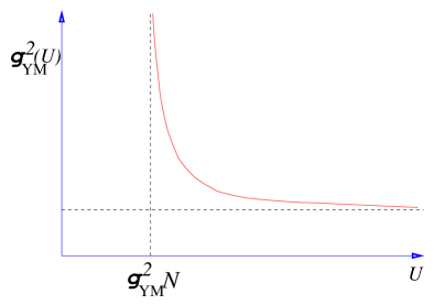
Figure 1: The running gauge coupling.

The coupling diverges at the scale $U=g^{2}_{\rm YM}N$. This should be the scale at which the $SU(N)$ is restored, but in fact it is not, since the divergence happens at $U\neq 0$. In other words, the branes are not coincident, and so (extending the discussion to any of the constituent branes), the generic gauge group is $U(1)^{N-1}$: we are out on the Coulomb branch of the gauge theory, and the origin is modified from being an $SU(N)$ point by quantum corrections.

3 Moduli Space Metrics

What we looked at just now was a four dimensional submanifold of the full $4N-4$ dimensional moduli space of the $SU(N)$ gauge theory. This full moduli space, which is hyperKähler, is proposed to be isomorphic to the relative moduli space^? of $N$ BPS monopoles of 4D $SU(2)$ gauge theory spontaneously broken to $U(1)$.^?,?,? Here, the wrapped D6–branes play the role of the monopoles, since they couple magnetically to the $U(1)$ which gets enhanced to an $SU(2)$ when $V(r)=V^{*}$. (There are 23 other $U(1)$’s which will not concern us here.) In the directions perpendicular to the wrapped brane, with coordinates $(r,\theta,\phi)$, they appear as monopoles in the $3+1$ dimensional problem.

So let us learn both about the gauge theory and the monopole moduli space. First let us consider the case of two monopoles $(N=2)$. In that case, it is known that the metric on the gauge theory moduli space is the Atiyah–Hitchin manifold, (as for the two monopole moduli space) which is given as follows:^?,?

$$ds^{2}_{\rm AH}=f^{2}d\rho^{2}+a^{2}\sigma_{1}^{2}+b^{2}\sigma_{2}^{2}+c^{2}\sigma_{3}^{2}\ ,\,\,\,{\rm where}$$

$$\qquad\sigma_{1}=-\sin\psi d\theta+\cos\psi\sin\theta d\phi\ ;$$

$$\qquad\sigma_{2}=\cos\psi d\theta+\sin\psi\sin\theta d\phi\ ;$$

$$\qquad\sigma_{3}=d\psi+\cos\theta d\phi\ ;$$

$${2bc\over f}{da\over d\rho} = (b-c)^{2}-a^{2}\ ,\mbox{ and cyclic perms.;}\quad\rho=2K\left(k\right),$$ (8)

and $K(k)$ is the elliptic integral of the first kind:

$$K(k)=\int_{0}^{\pi\over 2}(1-k^{2}\sin^{2}\tau)^{1\over 2}d\tau\ .$$ (9)

Also, $k$, the “modulus”, runs from $0$ to $1$, so $\pi\leq\rho\leq\infty$.

In our moduli space metric (7), if we rescale $\rho=U/g^{2}_{\rm YM}$ and $\psi=4\pi^{2}\sigma$, then we get:

$$ds^{2}={g^{2}_{\rm YM}\over 8\pi^{2}}ds^{2}_{\rm TN}\ ,\quad{\rm with}$$ (10)

$$ds^{2}_{\rm TN}=\left(1-{2\over\rho}\right)\left({d\rho}^{2}+\rho^{2}{d\Omega}^{2}_{2}\right)+4\left(1-{2\over\rho}\right)^{-1}\left({d\psi}+\cos\theta{d\phi}\right)^{2}\ .$$

This is precisely the form of the metric that one gets by expanding the Atiyah–Hitchin metric in large $\rho$. The difference between the Atiyah–Hitchin manifold and this “negative mass” ($m=-1$ in standard units, see e.g. ref.[15]) Taub–NUT metric is a family of exponential corrections of the form $e^{-\rho}$, which are non–perturbative in a large $\rho$ expansion.

From the point of view of the gauge theory, these corrections are of order $e^{-U/g^{2}_{\rm YM}}$, and so are instanton corrections. These corrections render the complete manifold smooth —the $\rho=2$ singularity is just an artifact of the large $\rho$ expansion— which is consistent with gauge theory expectations.

The combination $\psi=4\pi^{2}\sigma={\tilde{\sigma}}$ is the dual scalar to the gauge theory photon and has period $2\pi$. The fact that $\psi$ is $2\pi$ periodic and not $4\pi$ gives us an $SO(3)$ isometry for the Atiyah–Hitchin manifold instead of the naive $SU(2)$ of the Taub–NUT metric. In fact, it can be proven that the unique smooth hyperKähler manifold with this isometry and the above asymptotic behaviour is the Atiyah–Hitchin manifold, essentially proving that it is the correct result for the $SU(2)$ gauge theory moduli space.^?,?

What about $N$ different from 2? Well, the key observation^? is that the rescalings $\rho=2U/g^{2}_{\rm YM}N$ and $\psi=\sigma 8\pi^{2}/N$, give

$$ds^{2}={g^{2}_{\rm YM}N^{2}\over 32\pi^{2}}ds^{2}_{\rm TN}\ ,$$ (11)

generalising our previous result (3) connecting the moduli space metric to the same negative mass Taub–NUT spacetime. It is tempting to conclude that the manifold controlling our non–perturbative corrections for all $N$ is again the Atiyah–Hitchin manifold, but we should be careful. Note that changing $N$ will not change the period of the probe $U(1)$. ${\tilde{\sigma}}=4\pi^{2}\sigma$ should still have period $2\pi$. Therefore the period of $\psi$ in the metric above is now $4\pi/N$. Furthermore, the instanton corrections in the gauge theory will still be typically $e^{-U/g^{2}_{\rm YM}}$, and so this translates into $e^{-N\rho/2}$ for the corrections to the $m=-1$ Taub–NUT metric.

Let us then summarise what we have learned for our non–perturbative metrics for any $N$. They are Atiyah–Hitchin–like in the sense that:

$a)$ They differ from negative mass Taub–NUT by non–perturbative corrections of the form $e^{-N\rho/2}$.

$b)$ They have only a local $SU(2)$ action. Globally, it is broken by instanton corrections to $SU(2)/{\mathbf{Z}}_{N}$.

Some remarks are in order. One might worry that the manifolds that we seek might be singular, especially given property $b)$. This would be an awkward feature from the gauge theory perspective, since there is nothing like a Higgs branch available which might be opening up at the singularity, which is typically what happens in situations like this. (Classically there is no Higgs branch, and it seems imprudent to conjecture that one might be generated quantum mechanically.)

However, it is natural that there might be a harmless singularity in the moduli space following from the fact that we are studying a four dimensional subspace of the full $4N-4$ dimensional moduli space, which is known to be smooth. It is natural to expect that there are therefore $4N-8$ adjustable parameters in the full metric, which can resolve the singularity. The worry that the parameters do not appear in the metric written above is alleviated by the fact that these are non–perturbative parameters. They are monopole positions and phases: parameters of different vacua from the point of view of the one we have focussed on.

From the point of view of the monopole problem, or from the enhançon picture, this simply corresponds to the other monopoles which make up the internal structure of the $N-1$ monopole having to move around somewhat in order to accommodate the merging with the single monopole probe.

Property $a)$ also deserves some remarks. While the instanton corrections thus identified will smooth the singularity (together with the possible need for a resolution by adjusting $4N-8$ parameters) in the moduli space, it is clear that in the strict large $N$ limit, the corrections are extremely small because of the $N$ in the exponential. So in fact, the strict supergravity result for the location and nature of the enhançon is quite accurate. (See also ref.[20])

It is worth comparing this to the two monopole case ($N=2$). There, the naive singularity of the Taub–NUT metric is at $\rho=2$. It is in fact completely removed by non–perturbative effects, and the radius $\rho=\pi$ is the smallest possible value. This corresponds to the axisymmetric case of the two monopoles being exactly on top of one another.^? (This is naively a singularity of the complete metric but is in fact a “bolt” singularity, which is harmless.)

It is clear that there is a natural generalisation of this for each $N$. For very large $N$, the coincident monopole case is the enhançon itself, at $\rho=2$ of $U=g^{2}_{\rm YM}N$.

Another point worth making about large $N$ here is that while $\rho$ is a relative coordinate in the case of the two–monopole case, and the Taub–NUT and Atiyah–Hitchin manifolds have nothing to do with spacetime geometry, this is not true here: For large $N$, $\rho$ is a rescaled centre of mass coordinate of the $N-1$ monopole system being probed by a single one. But since $N$ is large, the centre of mass is essentially at the centre of the $N-1$ monopole, and so serves as a good spacetime coordinate, with the large monopole at the origin.

4 Fuzzy Geometry

Another appearance of the enhançon geometry is when a large number, $N$, of D3–branes are stretched between a pair of NS5–branes, as in figure 2(a).

                 

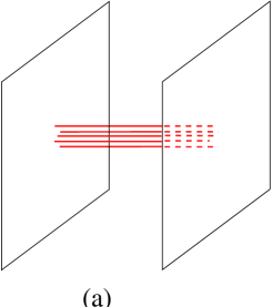
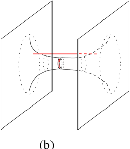
Figure 2: (a) A slice of the configuration of D3–branes stretching between NS5–branes. (b) A slice of the resulting “double trumpet” shape of the NS5–branes at large $N$. (A separated probe is also shown.) This system has a natural description in terms of the Nahm equations as explained in the text. The enhançon is the place (an $S^{2}$) where the NS5–branes touch.

This situation is related to the $K3$–wrapped D6–brane system by a chain of dualities.^? The D3–branes pull the NS5–branes into a shape such that at large $N$ they meet in an $S^{2}$ geometry, as in figure 2(b). This $S^{2}$ is the enhançon, since when two NS5–branes in type IIB string theory meet, there is an enhanced $SU(2)$ gauge symmetry describing their relative collective geometry. The endpoints of the D3–branes act as monopoles of the spontaneously broken $SU(2)$, where the Higgs vev is the asymptotic distance between the NS5–branes.

It is intuitively clear that in this and the wrapped D6–brane picture, the enhançon geometry is only a smooth sphere at large $N$. The geometry is made of $N$ smeared objects, the monopoles.

To find a quantitative description of this geometry needs new variables. In this D3/NS5 system, the variables are intuitive: $N$ D3–branes have 3 $N\times N$ matrix valued coordinates, $\Phi^{i}$ ($i=1,2,3$), representing their transverse motions within the NS5–brane worldvolumes. These coordinates are governed by Nahm’s equations in the BPS case:^?,?

$${d\Phi^{i}\over d\sigma}={1\over 2}\epsilon_{ijk}[\Phi^{j},\Phi^{k}]\ ,$$ (12)

where $\sigma\in[-1,1]$, (where we have placed the NS5–branes at $\pm 1$) and the appropriate solutions are those for which the $\Phi^{i}(\sigma)$ have a pole at the ends of the interval, with residues $\Sigma^{i}$, which form the $N\times N$ irreducible representation of $SU(2)$:^?,?,?

$$[\Sigma^{i},\Sigma^{j}]=2{\rm i}\epsilon^{ijk}\Sigma^{k}\ .$$ (13)

It is clear from this description that the D3–brane geometry has a non–commutative geometry underlying its description, the general solution taking one $SU(2)$ representation and twisting it into another while traversing the interval. A slice through this geometry, such as the enhançon itself at $\sigma=0$, is clearly a non–commutative or “fuzzy” sphere.^? As a simple attempt at creating an approximate solution, a symmetric “double trumpet” configuration can be made by gluing two sections of the infinite funnel solution of ref.[21]:

$$\Phi^{i}=f(\sigma)\Sigma^{i}\ ,\qquad f(\sigma)={g_{s}\over\sigma\pm 1}\ .$$ (14)

A complete solution would of course connect smoothly through the middle, but this crude solution serves to illustrate the point: A cross section of this is a fuzzy sphere, with radius $R$ given by:

$$R^{2}=4\pi^{2}\alpha^{\prime}\sum_{i=1}^{3}{\rm Tr}(\Phi^{i})^{2}=4\pi^{2}\alpha^{\prime}(N^{2}-1)f(\sigma)\ ,$$ (15)

giving a radius for the enhançon (at $\sigma=0$) of $R_{\rm e}\sim g_{s}\ell_{s}N$, which is we saw in the wrapped D6–brane description.

It is noteworthy that the geometry of this object made of expanding branes is described as a fuzzy sphere just as the brane expansion in a background R–R field produced by the dielectric brane effect.^? One is led to speculate that there might be further couplings to be deduced, such as multipole couplings to higher rank R–R fields via curvature terms on the D–brane worldvolume.

5 Other Branes and other Probes

Now although the wrapping of a D6–brane on $K3$ induces a negative D2–brane charge within the part of its worldvolume transverse to $K3$, it must be stressed that this is not an anti–D2–brane. It preserves the same supersymmetries that a D2–brane with that orientation would.

In fact, it is useful to consider adding extra D2–branes to the wrapped D6–brane arrangement with the same orientation as the unwrapped part of the D6–branes. Let us add $M$ of them. The net D2–brane charge as measured at infinity is therefore $M-N$, and it is interesting to note that we can cancel away the net charge by setting $M=N$.

There is an $SU(M)$ gauge theory on the worldvolume of these new branes, and there are of course strings which can stretch between these branes and the other set. Since these ones are not wrapped, the 2+1 dimensional gauge theory coupling is simply

$$g^{2}_{\rm YM,2}=g_{s}/\ell_{s}\ .$$ (16)

This form will produce an interesting conflict with the gauge theory coupling (1) of the wrapped brane gauge theory when we take decoupling limits shortly.

A natural question to ask is what happens to the geometry with the addition of these extra branes? Well, the first thing to note is that the supergravity geometry is simply modified by changing the harmonic function (4) which yields the D2–brane charge:

$$Z_{2}=1-\frac{(2\pi)^{4}g_{s}N\alpha^{\prime 5/2}}{2Vr}\longrightarrow{\widetilde{Z}}_{2}=1+\frac{(2\pi)^{4}g_{s}(M{-}N)\alpha^{\prime 5/2}}{2Vr}\ .$$ (17)

Note that this modifies, for example, the result for the volume of $K3$, which is now $V(r)=V{\widetilde{Z}}_{2}/Z_{6}$.

The next thing to notice is that we can probe with wrapped D6–branes as before, but we also can probe with pure D2–branes. The result for probing with a wrapped D6–brane is much like that which we saw before. It is equation (5), but now with

$$F(r)={Z_{6}\over 2g_{s}}\left(\mu_{6}V(r)-\mu_{2}\right)={1\over 2g_{s}}\left(\mu_{6}{\widetilde{Z}}_{2}-\mu_{2}Z_{6}\right)\ .$$ (18)

This means that everything we have seen is generically the same as before. There is an enhançon, which is still where $V(r)=V^{*}$, but for increasing $M$, this happens at smaller radius, given by:

$${\tilde{r}}_{\rm e}={V^{*}\over V-V^{*}}g_{s}\ell_{s}(N-M)\ .$$ (19)

After taking a decoupling limit, we will get similar results with $N$ replaced by $N-M$, and so, for example the scaled enhançon radius is ${\widetilde{U}}_{\rm e}=(N{-}M)g^{2}_{\rm YM}$. The result for probing with the pure D2–brane is easy to deduce. Take the previous results (5) and (18), set $\mu_{6}$ to zero, and reverse the sign of $\mu_{2}$. So we get in this case

$$F(r)={\mu_{2}Z_{6}\over 2g_{s}}\ .$$ (20)

So we see that the pure D2–branes completely ignore the D2–brane component, and we just get the usual result similar to that for D2–branes probing D6–branes in flat space. The effects of the wrapping on the transverse space simply do not show up. This is seen more clearly when one places this result for $F(r)$ into the metric (5) and see that it is essentially the Taub–NUT metric, now with a positive mass set by $N$. This will be precisely the case when we take a decoupling limit shortly.

So in fact the $M$ D2–branes which make up the geometry can clearly live at $r=0$, since there is no reason for them to be stuck at the enhançon radius. After excising the geometry interior to the radius $r_{\rm e}$, instead of replacing it with a flat geometry as we did before,^? we should replace it with a geometry produced by $M$ D2–branes in the interior, sitting at $r=0$, appropriately matched at ${\tilde{r}}_{\rm e}$ to the exterior geometry.

This is all made clearer when we take the decoupling limit of this result. Again we have a choice. We can take $\alpha^{\prime}\to 0$, holding $U=r/\alpha^{\prime}$ fixed, but we can choose to hold $a)$ the Yang–Mills coupling, (1) of the wrapped D6–branes, fixed, or $b)$ the coupling (16) on the pure D2–branes fixed. We cannot do both. The former stays with the wrapped D6–brane’s $SU(N)$ gauge theory, and treats the D2–branes as merely supplying extra hypermultiplets. The latter limit, instead, treats the D6–branes as hypermultiplets within the D2–brane $SU(M)$ gauge theory.

For the case $a)$ we get the metric in equation (7) with scaled function

$$f(U)={N\over 16\pi^{2}U}\ ,$$ (21)

a pure one loop contribution. Meanwhile, for case $b)$ we have instead the scaled function

$$f(U)={1\over 8\pi^{2}g^{2}_{\rm YM,2}}\left(1+{Ng^{2}_{\rm YM,2}\over 2U}\right)\ .$$ (22)

(It is interesting that one limit allows the tree level part to survive —coming from the “1” in the metric— while the other does not. The second case is reminiscent of an AdS–like limit.) The latter is precisely what one should get for the moduli space result. There is a $U(1)$ on the D2–brane and $N/2$ massless flavours supplied by the D6–branes.

With unwrapped D6–branes, we would have the following to say about the location $U=0$: The metric is smooth there for one flavour, as the NUT singularity is removable, but for higher numbers of flavours, the singularity is not removable (recall that the periodicity of $\sigma$ is fixed by the gauge theory), but has the happy interpretation of being the origin of a Higgs branch. This is the branch where the D2–brane becomes a fat instanton inside the D6–brane $SU(N)$ gauge theory. (More can be found out about this in refs.[28,29])

Here, with wrapped branes we have a subtlety. We have asked that we excise the naive spacetime geometry inside $r={\widetilde{r}}_{\rm e}$ (or $U={\widetilde{U}}_{\rm e}$), and replace it with a geometry which has no D6–branes inside that radius, so in fact there is no way to form instantons, and hence no Higgs branch. This appears to fit the fact that the D6–branes are wrapped on a small $K3$: we would need ${\mathbf{R}}^{4}$ to form genuine instantons.

Acknowledgements

CVJ would like to thank the organisers of the Strings 2000 conference at the University of Michigan for an invitation to present this work, and for an extremely enjoyable conference. A comment at the conference by Alex Buchel and an innocent–seeming question from an anonymous referee of ref.[3] are gratefully acknowledged.

References

References

- [1] J. Maldacena, Adv. Theor. Math. Phys. 2, 231 (1998), hep-th/9711200.
- [2] C. V. Johnson, A. Peet and J. Polchinski, Phys. Rev. D61 086001 (2000), hep-th/9911161.
- [3] C. V. Johnson, hep-th/0004068.
- [4] L. Järv and C. V. Johnson, hep-th/0002244, to appear in Phys. Rev. D.
-
[5]
K. Behrndt,
Nucl. Phys. B455, 188 (1995),
hep-th/9506106;
R. Kallosh and A. Linde, Phys. Rev. D52, 7137 (1995), hep-th/9507022;
M. Cvetič and D. Youm, Phys. Lett. B359, 87 (1995), hep-th/9507160. - [6] J. Polchinski, Phys. Rev. Lett. 75, 4724 (1995), hep-th/9510017.
- [7] C. V. Johnson, R. C. Myers, A. W. Peet and S. F. Ross, to appear.
-
[8]
E. J. Weinberg,
Phys. Rev. D20, 936 (1979);
W. Nahm, Phys. Lett. B85, 373 (1979). - [9] N. Seiberg and E. Witten, in “Saclay 1996, The mathematical beauty of physics” , hep-th/9607163.
- [10] G. Chalmers and A. Hanany, Nucl. Phys. B489, 223 (1997), hep-th/9608105.
- [11] A. Hanany and E. Witten, Nucl. Phys. B492, 152 (1997), hep-th/9611230.
- [12] N. Dorey, V. V. Khoze, M.P.Mattis, D. Tong and S. Vandoren, Nucl. Phys. B502, 59 (1997), hep-th/9703228.
- [13] M. F. Atiyah and N. J. Hitchin, “The Geometry And Dynamics Of Magnetic Monopoles.”, M.B. Porter Lectures, Princeton University Press (1988).
- [14] G. W. Gibbons and N. S. Manton, Nucl. Phys. B274 (1986) 183.
- [15] T. Eguchi, P. B. Gilkey and A. J. Hanson, Phys. Rept. 66, 213 (1980).
- [16] W. Nahm, “The Construction Of All Selfdual Multi - Monopoles By The ADHM Method. (Talk)”, in N. S. Craigie, P. . Goddard and W. . Nahm, “Monopoles In Quantum Field Theory. Proceedings, Monopole Meeting, Trieste, Italy, December 11-15, 1981”, World Scientific (1982).
- [17] D. Diaconescu, Nucl. Phys. B503, 220 (1997), hep-th/9608163.
- [18] J. Madore, Annals Phys. 219, 187 (1992); Class. Quant. Grav. 9, 69 (1992); Phys. Lett. B263, 245 (1991).
- [19] R. S. Ward, Commun. Math. Phys. 79 (1981) 317; Phys. Lett. B102, 136 (1981); Commun. Math. Phys. 83 563 (1982).
- [20] M. R. Douglas and S. H. Shenker, Nucl. Phys. B447, 271 (1995), hep-th/9503163.
- [21] N. R. Constable, R. C. Myers and O. Tafjord, Phys. Rev. D61, 106009 (2000).
- [22] N. Hitchin, Commun. Math. Phys. 83 579 (1982); Commun. Math. Phys. 89 148 (1982).
- [23] H. Nakajima, “Monopoles And Nahm’s Equations”, in Sanda 1990, Proceedings, Einstein metrics and Yang-Mills connections* 193-211.
- [24] D. Tsimpis, Phys. Lett. B433, 287 (1998), hep-th/9804081.
- [25] R. C. Myers, JHEP 9912, 022 (1999), hep-th/9910053.
- [26] M. Bershadsky, C. Vafa and V. Sadov, Nucl. Phys. B463, 398 (1996), hep-th/9510225.
-
[27]
E. B. Bogomolny,
Sov. J. Nucl. Phys. 24, 449 (1976);
M. K. Prasad and C. M. Sommerfield, Phys. Rev. Lett. 35, 760 (1975). - [28] N. Seiberg, Phys. Lett. B384, 81 (1996), hep-th/9606017.
- [29] C. V. Johnson, “D–Brane Primer”, hep-th/0007170.
- [30] C. V. Johnson and R. C. Myers, to appear.