Canonical and quantum FRW cosmological solutions in M-theory

Abstract

We present the canonical and quantum cosmological investigation of a spatially flat, four-dimensional Friedmann-Robertson-Walker (FRW) model that is derived from the M-theory effective action obtained originally by Billyard, Coley, Lidsey and Nilsson (BCLN). The analysis makes use of two sets of canonical variables, the Shanmugadhasan gauge invariant canonical variables and the “hybrid” variables which diagonalise the Hamiltonian. We find the observables and discuss in detail the phase space of the classical theory. In particular, a region of the phase space exists that describes a four-dimensional FRW spacetime first contracting from a strong coupling regime and then expanding to a weak coupling regime, while the internal space ever contracts. We find the quantum solutions of the model and obtain the positive norm Hilbert space of states. Finally, the correspondence between wave functions and classical solutions is outlined.

1 Introduction

The search for a theory of quantum gravity constitutes one of the uppermost challenges in theoretical high energy physics. The need for quantum gravity finds its roots within Einstein general relativity. Powerful general theorems [1] imply that our universe must have started from an initially singular state with infinite curvature. In such circumstances, where the laws of classical physics break down, it is unclear how any boundary conditions necessary for a description of a dynamical system could have been imposed at the initial singularity. Quantum corrections could induce a modification of classical general relativity and strongly influence the evolution of the very early universe [2].

In the last two decades superstring theory [3] has emerged as a successful candidate for the theory of quantum gravity. In cosmology, most of the modifications to general relativity induced by superstring theory are originated by the inclusion of the dilaton, axion and various moduli fields, together with higher curvature terms that are present in the low-energy effective actions. Each of these novel ingredients do indeed lead to new cosmological solutions. A remarkable example is given by the so-called pre-big bang cosmologies [4] that are derived by the low-energy effective string action. Different branches of the solution are related by time reflection and internal transformations – $O(d,d)$ and, in particular, scale factor duality – that follow from the $T$-duality property of the full superstring theory [5]. According to the pre-big bang scenario the universe evolves from a weak coupled string vacuum state to a radiation-dominated and then matter-dominated FRW geometry through a region of strong coupling and large curvature. Although the pre-big bang model has not yet proven able to solve all its pitfalls, such as the existence of a singular boundary that separates the pre- and post-big bang branches [6], it provides a good starting point to investigate high-energy cosmology.

Recently, it has become evident that the five consistent, anomaly free, perturbative formulations of ten-dimensional superstring theories are connected by a web of duality transformations [3] and constitute special points of a large, multi-dimensional moduli space of a more fundamental (non-perturbative) theory, designated as M-theory [7]. Quite interestingly, it happens that another point of the M-theory moduli space corresponds to eleven-dimensional supergravity, the low-energy limit of M-theory [7, 8]. Assuming that M-theory is the ultimate theory of quantum gravity, it is natural to begin exploring its cosmological implications. Although our understanding of M-theory is still incomplete, there are hopes that some of the obstacles of dilaton driven inflation in string theory could be overcome within the new theory. The underlying idea is to investigate the dynamics at the extreme weak- and strong-coupling regimes of superstring theory from a M-theory perspective, where the existence of eleven dimensions seems mandatory.

Several different approaches to M-theory cosmology have already been explored in the literature [9],[10],[12]-[17]. In the framework of the Hořava-Witten model [11], M-theory and cosmology have been combined in the works of Lukas, Ovrut and Waldram [9]. A somewhat related line of research is the brane world by Randall and Sundrum [10], where our four-dimensional universe emerges as the world volume of a three-brane in a higher-dimensional spacetime. From a different point of view, Damour and Henneaux have investigated chaotic models [12] and Lu, Maharana, Mukherji and Pope have discussed classical and quantum M-theory models with homogeneous graviton, dilaton and antisymmetric tensor field strengths [13]. Different classes of cosmological solutions that reduce to solutions of string dilaton gravity have been discussed in Ref. [14]-[16]. In particular, a global analysis of four-dimensional cosmologies derived from M-theory and type $IIA$ superstring theory has been presented by BCLN [17]. Using the theory of dynamical systems to determine the qualitative behaviour of the solutions, the authors find that form-fields associated with the NS/NS and R/R sectors play a rather crucial role in determining the dynamical behaviour of the solutions: the R/R fields cause the universe to collapse but the NS/NS fields, such as the axion, have opposite effect. Quite interestingly, for flat FRW models the boundary of the classical physical phase space is a set of invariant submanifolds, where either the axion field is trivial or the four-form field strength is dynamically unimportant. This interplay leads to important consequences, as the orbits in the phase space are dominated by the dynamics associated with one, or the other, or both invariant submanifolds in sequence, shadowing trajectories in the invariant submanifold [17].

In this paper we discuss the main scenario introduced by BCLN from a canonical perspective. This approach allows us to analyse in depth the physical properties of the classical solutions and to obtain a consistent quantum description of the model. We consider the bosonic sector of eleven-dimensional supergravity which consists of a graviton and an antisymmetric three-form potential. The theory is compactified to four dimensions by assuming a geometry of the form $M^{4}\times T^{6}\times S^{1}$, where $T^{6}$ is a six-dimensional torus and $M^{4}$ corresponds to a spatially flat FRW spacetime. The effective theory in four dimensions bears a dilaton $\phi$, a modulus field $\beta$ identifying the internal space, a pseudo-scalar axion field $\sigma$ and a potential term induced by a four-form field. [See Eq. (5) below.] A brief derivation of the previous steps is presented in Section 2, where the two invariant submanifolds are identified. In Section 3 we analyse the first invariant submanifold, where the four-form field is negligible and the axion field dominates. In particular, in Subsection 3.1 we discuss the parameter space of the classical theory and in Subsection 3.2 we find the Hilbert space of states of the quantum theory. This programme is performed by using two sets of canonical variables, the so-called Shanmugadhasan variables [18] (forming a maximal set of gauge invariant variables) and the “hybrid” variables that diagonalise the Hamiltonian. In Section 4, we repeat the analysis of Section 3 for the invariant manifold with negligible axion field and dominant four-form field. Finally, our conclusions are presented in Section 5. Two appendixes contain technical details and complete the paper.

2 M-theory cosmology

In this section we closely follow Ref. [17] and derive the four-dimensional minisuperspace effective actions that will be used to discuss the dynamics of M-theory cosmology.

The bosonic sector of eleven-dimensional supergravity action $S^{(11)}$ is

$$S^{(11)}=\int d^{11}X\sqrt{-g^{(11)}}\left[R^{(11)}(g^{(11)}_{ab})-{1\over 48}F_{a_{1}\dots a_{4}}F^{a_{1}\dots a_{4}}\right.$$

$$\qquad\qquad\left.-{1\over 12^{4}\sqrt{-g^{(11)}}}\epsilon^{a_{1}\dots a_{3}b_{1}\dots b_{4}c_{1}\dots c_{4}}A_{a_{1}\dots a_{3}}F_{b_{1}\dots b_{4}}F_{c_{1}\dots c_{4}}\right]\,,$$ (1)

where $a_{i},b_{i},c_{i}=0\dots 10$, $F_{a_{1}\dots a_{4}}=4\partial_{[a_{1}}A_{a_{2}\dots a_{4}]}$ is the four-form field strength of the antisymmetric three-form potential $A_{a_{1}\dots a_{3}}$, and $g^{(11)}$ denotes the determinant of the eleven-dimensional metric $g^{(11)}_{ab}$. Equation (1) describes the low-energy limit of M-theory [7, 8].

The four-dimensional effective action is derived from Eq. (1) by a sequence of two Kaluza-Klein compactifications, on a circle $S^{1}$ with radius $R_{S^{1}}=e^{\Phi_{10}/3}$ and on an isotropic six-torus with volume $V_{T^{6}}=e^{6\beta}$, respectively. The eleven-dimensional metric is

$$ds^{2}_{(11)}\equiv g^{(11)}_{ab}dX^{a}dX^{b}=e^{-\Phi_{10}/3}[g_{\mu\nu}dx^{\mu}dx^{\nu}+e^{2\beta}\delta_{ij}dx^{i}dx^{j}]+e^{2\Phi_{10}/3}dX_{10}^{2}\,,$$ (2)

where $\mu,\nu=0\dots 3$ and $i,j=4\dots 9$. The first compactification gives the ten-dimensional effective action for the massless type IIA superstring [7, 20]

$$S^{(10)}=\int d^{10}x\sqrt{-g^{(s)}}\left[e^{-\Phi_{10}}\left(R^{(10)}(g^{(s)}_{mn})+\left(\nabla\Phi_{10}\right)^{2}-{1\over 12}H_{mnp}H^{mnp}\right)\right.$$

$$\qquad\qquad\left.-\frac{1}{48}F_{mnpq}F^{mnpq}-{1\over 384\sqrt{-g^{(11)}}}\epsilon^{m_{1}m_{2}n_{1}\dots n_{4}p_{1}\dots p_{4}}B_{m_{1}m_{2}}F_{n_{1}\dots n_{4}}F_{p_{1}\dots p_{4}}\right]\,,$$ (3)

where $g^{(s)}_{mn}=(g_{\mu\nu},e^{2\beta}\delta_{ij})$, and $H_{mnp}$ and $F_{mnpq}$ are the field strengths of the potentials $B_{np}$ and $A_{npq}$, respectively. Assuming that the only non-trivial components of the form fields are those associated with $M^{4}$ the second compactification gives the effective four-dimensional action [17]

$$S=\int d^{4}x\sqrt{-g}\left[e^{-\Phi_{4}}\left(R^{(4)}(g_{\mu\nu})+\left(\nabla\Phi_{4}\right)^{2}-6\left(\nabla\beta\right)^{2}-{1\over 12}H_{\mu\nu\lambda}H^{\mu\nu\lambda}\right)-{1\over 48}e^{6\beta}F_{\mu\nu\lambda\kappa}F^{\mu\nu\lambda\kappa}\right]\,,$$ (4)

where the four-dimensional dilaton field is $\Phi_{4}=\Phi_{10}-6\beta$. Finally, solving the field equation for the four-form $F^{\mu\nu\lambda\kappa}$ and dualizing the three-form $H^{\mu\nu\lambda}$, Eq. (4) can be cast in the form

$$S=\int d^{4}x\sqrt{-g}\left[e^{-\Phi_{4}}\left(R^{(4)}(g_{\mu\nu})+\left(\nabla\Phi_{4}\right)^{2}-6\left(\nabla\beta\right)^{2}-{1\over 2}e^{2\Phi_{4}}\left(\nabla\sigma\right)^{2}\right)-{1\over 2}Q^{2}e^{-6\beta}\right]\,,$$ (5)

where $\sigma$ is the pseudo-scalar axion field dual to the three-form, $H^{\mu\nu\lambda}=e^{\Phi_{4}}\epsilon^{\mu\nu\lambda\kappa}\nabla_{\kappa}\sigma$, and $F^{\mu\nu\lambda\kappa}=Qe^{-6\beta}\epsilon^{\mu\nu\lambda\kappa}$. Equation (5) is our starting point to investigate classical and quantum four-dimensional M-theory cosmology.

Since we are interested in homogeneous and isotropic four-dimensional cosmologies the ansatz for the four-dimensional section of the (string frame) metric (2) is

$$ds^{2}_{(4)}\equiv g_{\mu\nu}dx^{\mu}dx^{\nu}=-N^{2}(t)dt^{2}+e^{2\alpha(t)}d\Omega_{3k}\,,\qquad N(t)>0$$ (6)

where $d\Omega_{3k}$ is the maximally symmetric three-dimensional unit metric with curvature $k=0,\pm 1$, respectively. By substituting Eq. (6) in Eq. (5) and requiring that the modulus field $\beta$, the dilaton $\Phi_{4}$, and the axion $\sigma$ depend only on $t$, the action (5) becomes

$$S=\int dt\,\left[{1\over\mu}\left(3\dot{\alpha}^{2}-\dot{\phi}^{2}+6\dot{\beta}^{2}+{1\over 2}\dot{\sigma}^{2}e^{2(3\alpha+\phi)}\right)+\mu\left(6ke^{-2(\alpha+\phi)}-{1\over 2}Q^{2}e^{3\alpha-\phi-6\beta}\right)\right]\,,$$ (7)

where we have defined the “shifted dilaton” field

$$\phi=\Phi_{4}-3\alpha\,,$$ (8)

and the Lagrange multiplier

$$\mu(t)=Ne^{\phi}>0\,.$$ (9)

The dynamics of the action (7) has been discussed qualitatively in Ref. [17]. Here we restrict attention to spatially flat spacetimes ($k=0$) and discuss in detail two subcases of Eq. (7) that turn out to be completely integrable:

• The invariant submanifold

  $$S_{I}=\int dt\,\left[{1\over\mu}\left(3\dot{\alpha}^{2}-\dot{\phi}^{2}+6\dot{\beta}^{2}+{1\over 2}\dot{\sigma}^{2}e^{2(3\alpha+\phi)}\right)\right]\,,$$ (10)

  which is obtained from Eq. (7) by setting $Q=0$ and $k=0$. This case describes spatially flat low-energy M-theory cosmology with negligible four-form $F^{\mu\nu\lambda\kappa}$. The general solution for this model (including spatially curved models which are not discussed here) was first discussed by Copeland, Lahiri and Wands in Ref. [15].

• The invariant submanifold

  $$S_{II}=\int dt\,\left[{1\over\mu}\left(3\dot{\alpha}^{2}-\dot{\phi}^{2}+6\dot{\beta}^{2}\right)-{1\over 2}\mu\,Q^{2}e^{3\alpha-\phi-6\beta}\right]\,.$$ (11)

  which is obtained from Eq. (7) by setting $\sigma=constant$ and $k=0$. This case describes spatially flat low-energy M-theory cosmology with trivial axion field.

The intersection of the two invariant submanifolds I and II further identifies the invariant submanifold

$$S_{I\cap II}=\int dt\,\left[{1\over\mu}\left(3\dot{\alpha}^{2}-\dot{\phi}^{2}+6\dot{\beta}^{2}\right)\right]\,.$$ (12)

In the following two sections we will discuss the classical and quantum dynamics of the invariant submanifolds I and II, respectively. The degenerate case $S_{I\cap II}$ will be outlined at the end of Section 4.

3 Invariant submanifold I

Equation (10) can be cast in the canonical form

$$S_{I}=\int dt\left[\dot{\alpha}p_{\alpha}+\dot{\phi}p_{\phi}+\dot{\beta}p_{\beta}+\dot{\sigma}p_{\sigma}-{\cal H}\right]\,,$$ (13)

where the Hamiltonian is

$${\cal H}=\mu H\,,\qquad H={1\over 24}\left(2p^{2}_{\alpha}-6p^{2}_{\phi}+p^{2}_{\beta}+12p^{2}_{\sigma}e^{-2(3\alpha+\phi)}\right)\,.$$ (14)

As is expected for a time-reparametrization invariant system, the total Hamiltonian ${\cal H}$ is proportional to the non-dynamical variable $\mu$ [21, 22]. The latter enforces the constraint

$$H=0\qquad\to\qquad 2p_{\alpha}^{2}-6p^{2}_{\phi}+p^{2}_{\beta}+12p^{2}_{\sigma}e^{-2(3\alpha+\phi)}=0\,.$$ (15)

The canonical equations of motion are

$$\begin{array}[]{llll}\displaystyle\dot{\alpha}={p_{\alpha}\over 6}\,,&\displaystyle\dot{\phi}=-{p_{\phi}\over 2}\,,&\displaystyle\dot{\beta}={p_{\beta}\over 12}\,,&\displaystyle\dot{\sigma}=p_{\sigma}e^{-2(3\alpha+\phi)}\,,\\ \\ \displaystyle\dot{p}_{\alpha}=3p_{\sigma}^{2}e^{-2(3\alpha+\phi)}\,,&\displaystyle\dot{p}_{\phi}=p_{\sigma}^{2}e^{-2(3\alpha+\phi)}\,,&\displaystyle\dot{p}_{\beta}=0\,,&\displaystyle\dot{p}_{\sigma}=0\,,\end{array}$$ (16)

where the dots represent differentiation w.r.t. gauge parameter

$$\tau(t)=\int_{t_{0}}^{t}\mu(t^{\prime})dt^{\prime}\,,\qquad t>t_{0}\,,$$ (17)

where $t_{0}$ is an arbitrary constant. Note that since $\mu$ is positive defined $\tau(t)$ is a monotone increasing function.

Different choices of $\mu$ correspond to different choices of time. We have the following interesting time parameters:

• Cosmic proper time $t_{c}$. The cosmic proper time is defined by the condition $N=1$. It is obtained by choosing

  $$\mu(\tau)\equiv\left[{dt_{c}\over d\tau}\right]^{-1}=e^{\phi}\,,$$ (18)

  which leads to

  $$t_{c}(\tau)=\int_{-\infty}^{\tau}d\tau\,e^{-\phi(\tau^{\prime})}\,,$$ (19)

  where we have chosen the arbitrary constant so that $t(-\infty)=0$.

• Gauge proper time $t_{g}$. The gauge proper time is defined by the condition $\mu=1$. This leads to

  $$t_{g}(\tau)=\tau-\tau_{0}\,.$$ (20)

  This is the natural time parameter to discuss the classical dynamics and the quantization of the model.

• The BCLN time variable $\eta$. This is defined by the condition

  $${d\eta\over dt_{c}}\equiv e^{(3\alpha+\phi-6\beta)/2}\,,$$ (21)

  or, using Eq. (19),

  $${d\eta\over d\tau}=e^{(3\alpha-\phi-6\beta)/2}\,,$$ (22)

• The BCLN dimensionless time variable $\tau_{\scriptscriptstyle BCLN}$

  $${d\tau_{\scriptscriptstyle BCLN}\over d\eta}={d\phi\over d\eta}\,,\quad\to\quad\tau_{\scriptscriptstyle BCLN}-\tau_{\scriptscriptstyle BCLN}{}_{0}=\phi\,.$$ (23)

The choices iii) and iv) are useful to compare the notations used in this paper to those of Ref. [17]. This is done in Appendix A.

3.1 Classical solutions

The off-shell solution of the canonical equations is

$$\begin{array}[]{lll}\alpha&=&\displaystyle\alpha_{0}+{1\over 2}\ln\left[\cosh\left(\kappa(\tau-\tau_{0})\right)\right]-\xi(\tau-\tau_{0})\,,\\ \\ p_{\alpha}&=&\displaystyle 3\kappa\tanh\left[\kappa(\tau-\tau_{0})\right]-6\xi\,,\\ \\ \phi&=&\displaystyle\phi_{0}-{1\over 2}\ln\left[\cosh\left(\kappa(\tau-\tau_{0})\right)\right]+3\xi(\tau-\tau_{0})\,,\\ \\ p_{\phi}&=&\displaystyle\kappa\tanh\left[\kappa(\tau-\tau_{0})\right]-6\xi\,,\\ \\ \beta&=&\displaystyle\beta_{0}+{p_{\beta}\over 12}(\tau-\tau_{0})\,,\\ \\ p_{\beta}&=&{\rm constant}\,,\\ \\ \sigma&=&\displaystyle\sigma_{0}+{\kappa\over p_{\sigma}}\tanh\left[\kappa(\tau-\tau_{0})\right]\\ \\ p_{\sigma}&=&{\rm constant}\,,\end{array}$$

where $\alpha_{0}$, $\phi_{0}$, $\beta_{0}$, $\sigma_{0}$ and $\tau_{0}$ are constants of integration,

$$\kappa^{2}-12\xi^{2}+{p_{\beta}^{2}\over 12}=2H\,,\qquad\kappa\not=0\,,$$ (24)

and (we choose $\kappa>0$ for simplicity)

$$3\alpha_{0}+\phi_{0}=\ln\left({|p_{\sigma}|\over\kappa}\right)\,.$$ (25)

On the (physical) shell $\xi=0$ is a degenerate trivial configuration of the system because it implies $\kappa=0$ and $p_{\beta}=0$.

Since the model is integrable we can find a maximal set of gauge invariant observables. The system is invariant under reparametrizations of time so we expect six physical gauge invariant observables. (Indeed, the system possesses four canonical degrees of freedom and thus the general solution is determined by eight constant of motion: the constraint $H$, the initial value of the gauge parameter $\tau$, and six other constant quantities which are the observables of the system.) Considering the off-shell solution a possible choice is

$$\begin{array}[]{lll}\displaystyle U=\alpha+\phi+{3p_{\phi}-p_{\alpha}\over 6\kappa}\,{\rm arccosh}\,\left({\kappa\over|p_{\sigma}|}e^{\phi+3\alpha}\right)\,,&&\displaystyle V={1\over 2}\left(3p_{\phi}-p_{\alpha}\right)\,,\\ \\ \displaystyle X=\beta-{p_{\beta}\over 12\kappa}\,{\rm arccosh}\,\left({\kappa\over|p_{\sigma}|}e^{\phi+3\alpha}\right)\,,&&\displaystyle W=p_{\beta}\,,\\ \\ \displaystyle Y=\sigma-{p_{\alpha}-p_{\phi}\over 2p_{\sigma}}\,,&&\displaystyle Z=p_{\sigma}\,,\end{array}$$ (26)

where

$$\kappa=\left[{1\over 4}\left(p_{\alpha}-p_{\phi}\right)^{2}+p_{\sigma}^{2}e^{-2(3\alpha+\phi)}\right]^{1/2}\,.$$ (27)

The quantities (26), being gauge invariant, have vanishing Poisson brackets with the Hamiltonian (14) and have been chosen such that the only nonvanishing Poisson brackets are

$$\begin{array}[]{lllll}\left[U,V\right]_{P}=1\,,&&\left[X,W\right]_{P}=1\,,&&\left[Y,Z\right]_{P}=1\,.\end{array}$$ (28)

The set of gauge invariant quantities (26) can be completed by the Hamiltonian $H$ and by its canonically conjugate ($[T,H]_{P}=1$)

$$T={1\over\kappa}\,{\rm arccosh}\,\left({\kappa\over|p_{\sigma}|}e^{\phi+3\alpha}\right)$$ (29)

to obtain a maximal set of canonical variables (also called Shanmugadhasan variables [18]). Note that the quantity $T$ has been chosen to have vanishing Poisson brackets with the observables (26). Since $[T,H]_{P}=1$, $T$ transforms linearly under gauge transformations generated by the constraint. This will be useful in the following.

For sake of completeness, let us write the relation between the gauge invariant observables and the constants of motion in Eqs. (3.1). Using Eqs. (14), (26) and (29), after a bit of algebra we find

$$\begin{array}[]{c}\displaystyle\alpha_{0}={1\over 2}\ln{|p_{\sigma}|\over\kappa}-{1\over 2}U\,,\quad\phi_{0}=-{1\over 2}\ln{|p_{\sigma}|\over\kappa}+{3\over 2}U\,,\quad\beta_{0}=X\,,\quad\sigma_{0}=Y\,,\\ \\ \displaystyle\xi=-{1\over 6}V\,,\quad p_{\beta}=W\,,\quad p_{\sigma}=Z\,,\quad\kappa=\left[{1\over 12}(4V^{2}-W^{2})+2H\right]^{1/2}\,.\end{array}$$ (30)

Another useful canonical chart is formed by the hybrid variables that diagonalise the constraint (15). Although the hybrid variables are not (all) gauge invariant they allow to fix a global gauge and quantize exactly the system. The hybrid variables $(a,b,c,\sigma)$ are defined by the canonical transformation

$$\begin{array}[]{lll}\displaystyle a=\phi+3\alpha\,,&\displaystyle b=\sqrt{3}(\phi+\alpha)\,,&\displaystyle c=2\sqrt{3}\beta\,,\\ \\ \displaystyle p_{a}={1\over 2}\left(p_{\alpha}-p_{\phi}\right)\,,&\displaystyle p_{b}={1\over 2\sqrt{3}}\left(3p_{\phi}-p_{\alpha}\right)\,,&\displaystyle p_{c}={1\over 2\sqrt{3}}p_{\beta}\,.\end{array}$$ (31)

Note that $a$ coincides with the four-dimensional dilaton field $\Phi_{4}$. Using the hybrid variables the constraint (15) reads (we have divided by a factor $12$)

$$p_{a}^{2}-p^{2}_{b}+p^{2}_{c}+p^{2}_{\sigma}e^{-2a}=0\,.$$ (32)

The gauge invariant canonical variables are related to the hybrid variables by the canonical transformation

$$\begin{array}[]{ll}\displaystyle U={1\over\sqrt{3}}\left[b+{p_{b}\over\kappa}\,{\rm arccosh}\,\left({\kappa\over|p_{\sigma}|}e^{a}\right)\right]\,,&\displaystyle V=\sqrt{3}p_{b}\,,\\ \\ \displaystyle X={1\over 2\sqrt{3}}\left[c-{p_{c}\over\kappa}\,{\rm arccosh}\,\left({\kappa\over|p_{\sigma}|}e^{a}\right)\right]\,,&\displaystyle W=2\sqrt{3}p_{c}\,,\\ \\ \displaystyle Y=\sigma-{p_{a}\over p_{\sigma}}\,,&\displaystyle Z=p_{\sigma}\,,\\ \\ \displaystyle T={1\over\kappa}\,{\rm arccosh}\,\left({\kappa\over|p_{\sigma}|}e^{a}\right)\,,&\displaystyle H={1\over 2}\left(p_{a}^{2}-p^{2}_{b}+p^{2}_{c}+p^{2}_{\sigma}e^{-2a}\right)\,,\end{array}$$ (33)

where $\kappa=\sqrt{p_{a}^{2}+p_{\sigma}^{2}e^{-2a}}$. The canonical transformation above is generated by the generating function of the first kind [19]

$$F_{1}(a,b,c,\sigma;U,X,Y,T)={1\over 2T}\left[(\sqrt{3}U-b)^{2}-(2\sqrt{3}X-c)^{2}-\,{\rm arccosh}\,^{2}\sqrt{1+e^{2a}(Y-\sigma)^{2}}\right]\,.$$ (34)

Let us now discuss the behaviour of the classical solution. The on-shell classical solution is determined by six physical parameters. From the equations of motion we see that five of them ($\alpha_{0}$, $\phi_{0}$, $\beta_{0}$, $\sigma_{0}$, and $\tau_{0}$) give initial conditions for the canonical variables and do not influence the qualitative behaviour of the solution. Therefore, the qualitative dynamics of the model is determined by a two-dimensional parameter space described by two coordinates, for instance $\kappa$ and $\xi$. Using $\kappa$ and $\xi$ as free parameters, from Eq. (24) it follows that $p_{\beta}$ is (on-shell)

$$p_{\beta}=\pm{2\sqrt{3}}\sqrt{12\xi^{2}-\kappa^{2}}\,.$$ (35)

The sign of $p_{\beta}$ determines the dynamical behaviour of the internal six-torus space. In fact, from the solution of the equations of motion one obtains the scale factor of the internal space (we set $\tau_{0}=0$ for simplicity)

$$R_{T^{6}}\equiv e^{\beta}=e^{\beta_{0}}\cdot e^{p_{\beta}\tau/12}\,.$$ (36)

Physically, we want compactification at late (cosmic) times. Compactification of the six-torus space is achieved for $p_{\beta}\leq 0$. Indeed, for negative values of $p_{\beta}$ $\lim_{\tau\to\infty}R_{T^{6}}=0$, i.e., the internal space shrinks to zero for large values of the gauge proper time, while decompatifying for $\tau\to-\infty$ when the strong coupling region of the theory is approached. Since the relation between the cosmic proper time and the gauge proper time is monotone [see Eq. (19)] the dynamics in $\tau$ is identical to the dynamics in $t_{c}$, and the internal space shrinks to zero for large values of the cosmic proper time as well. Note that the gauge proper time is defined in the interval $\tau\in]-\infty,\infty[$ whereas $t_{c}$ is defined only on the half line. The limiting value $p_{\beta}=0$ corresponds to a constant (stable) internal space with radius $R_{T^{6}}=e^{\beta_{0}}$ and is physically acceptable for sufficiently large negative values of $\beta_{0}$. In the following we will restrict attention to nonpositive values of $p_{\beta}$, the extension to $p_{\beta}>0$ being straightforward (see Fig. 1).

At fixed $\kappa$ we distinguish three different dynamical behaviours of the four-dimensional external space according to the value of $\xi$:

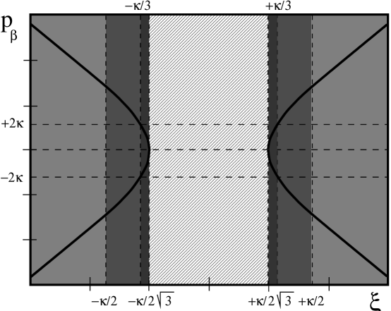
Figure 1: Parameter space for invariant submanifold I. The physical points are represented by the two branches of the hyperbola (35). The different colored regions determine on the two branches of the hyperbola the different physical cases described in the text.

• $\xi\leq-\kappa/2$ ($p_{\beta}<-2\kappa$). In this case the external scale factor ever expands while the internal scale factor shrinks from infinity to zero. The Hubble parameter is always positive and vanishes asymptotically at large times. In particular, for $\xi=-\kappa/2$ the external space starts at $\tau=-\infty$ ($t_{c}=0$) with a finite nonzero scale factor and vanishing Hubble parameter. For $\xi<-\kappa/2$ the external space starts with a vanishing scale factor and infinite Hubble parameter, which is always decreasing. $\tau=-\infty$ ($t_{c}=0$) is the strong coupling region where the coupling constants of the theory, $g=\exp(\phi)$ and $g_{10}=\exp(\Phi_{10})$, become infinite. Conversely, $\tau=\infty$ ($t_{c}=\infty$) is the weak region coupling where both $g$ and $g_{10}$ vanish. $g$ and $g_{10}$ are always decreasing. (See Fig. 2.)

    

  Figure 2: Graphical representation of the dynamics of the invariant submanifold I for $\xi<-\kappa/2$ as function of the gauge proper time $t_{g}$ and of the cosmic proper time $t_{c}$. [Here and in the following figures we set $\alpha_{0}=\phi_{0}=\beta_{0}=0$ for simplicity.] The solid and dashed lines describe the evolution of the radius of the external spacetime and of the internal space, respectively. The dotted and dash-dotted lines represent the evolution of the coupling constants $g$ and $g_{10}$, respectively.

• $\xi\geq\kappa/2$ ($p_{\beta}<-2\kappa$). In this case both the external scale factor and the internal scale factor ever contract. The Hubble parameter is always negative and asymptotically vanishing at small times ($\tau=-\infty$). In particular, for $\xi=\kappa/2$ the external space ends at $\tau=\infty$ ($t_{c}=0$) with a finite nonzero scale factor and vanishing Hubble parameter. For $\xi>\kappa/2$ the external space ends with a vanishing scale factor and infinite Hubble parameter. $g$ increases from zero at $\tau=-\infty$ ($t_{c}=-\infty$) to infinity at $\tau=\infty$ ($t_{c}=0$). Conversely, $g_{10}$ decreases from infinity to zero.

• $-\kappa/2<\xi<-\kappa/2\sqrt{3}$ and $\kappa/2\sqrt{3}<\xi<\kappa/2$. In this case the external scale factor first contracts then expands, bouncing from infinity to infinity. In particular, for

  • $-\kappa/2<\xi\leq-\kappa/3$ ($p_{\beta}<-2\kappa$) the internal scale factor shrinks from infinity to zero. The Hubble parameter starts with infinite negative value, becomes positive and then decreases to zero after having reached a positive maximum. $g$ and $g_{10}$ decrease from infinity to zero [$g_{10}$ to a finite nonzero positive value for the limiting value $\xi=-\kappa/3$] (see Fig. 3);

      

    Figure 3: Graphical representation of the dynamics of the invariant submanifold I for $-\kappa/2<\xi<-\kappa/3$ as function of the gauge proper time $t_{g}$ and of the cosmic proper time $t_{c}$. The internal scale factor and the coupling constant $g$ and $g_{10}$ are ever decreasing and vanish for large times. The external scale factor is large both at small and large times. (See Fig. 2 for the key to the plotted lines.)

  • $-\kappa/3<\xi\leq-\kappa/2\sqrt{3}$ the internal scale factor shrinks from infinity to zero [$-\kappa/3<\xi<-\kappa/2\sqrt{3}$ ($-2\kappa<p_{\beta}<0$)] or is constant [$\xi=-\kappa/2\sqrt{3}$ ($p_{\beta}=0$)].The Hubble parameter starts with infinite negative value, becomes positive and then decreases to zero after having reached a positive maximum. $g$ decreases from infinity to zero. $g_{10}$ bounces from infinity to infinity via a positive minimum;

  • $\kappa/2\sqrt{3}\leq\xi<\kappa/3$ ($-2\kappa<p_{\beta}<0$). The internal scale factor shrinks from infinity to zero [$\kappa/2\sqrt{3}<\xi<\kappa/3$ ($-2\kappa<p_{\beta}<0$)] or is constant [$\xi=\kappa/2\sqrt{3}$ ($p_{\beta}=0$)]. The Hubble parameter is first negative and small, decreases to a negative minimum and then increases to infinity. $g$ increases from zero to infinity. $g_{10}$ bounces from infinity to infinity via a positive minimum.

  • $\kappa/3\leq\xi<\kappa/2$ ($p_{\beta}<-2\kappa$). The internal scale factor shrinks from infinity to zero. The Hubble parameter is first negative and small, decreases to a negative minimum and then increases to infinity. $g$ increases from zero to infinity. $g_{10}$ decreases from infinity to zero for $\kappa/3<\xi<\kappa/2$ or to a finite nonzero positive value for the limiting value $\xi=\kappa/3$.

Several comments are in order about the dynamics of the dilaton-axion-moduli solution i)-iii). First of all, we do not find a two-branch solution as happens in the pre-big bang scenario [4]. Indeed, the action (10) (with $\dot{\sigma}\not=0$) is not invariant under scale factor duality and moreover the presence of the axion leads to an effective potential [see Eq. (32)] with opposite sign to that required for the pre-/post-big bang branches to exist. (See e.g. Gasperini, Maharana and Veneziano in Ref. [6].) Scenarios i) and iii) are most attractive as far as a physical description of our universe is concerned. According to i) the universe begins in a strong coupling region with large internal space. Actually, both the coupling constants, $g$ and $g_{10}$, and the radius of the internal six-torus are infinite at $t_{c}=0$. However, this is not disturbing because for $t_{c}\to 0$ the spacetime curvature blows up. So we are in the strong coupling regime of the theory and the low-energy description of M-theory given by eleven-dimensional supergravity breaks down. Hopefully, non-perturbative effects would cure the initial singularity. At small times ($t_{c}\approx 0$) the expansion of the external spacetime is characterized $H>>1$. Then the expansion slows down and at large times the Hubble parameter vanishes, approaching a standard FRW behaviour. At small cosmic times the scale factor of the external spacetime expands as

$$a(t_{c})\approx t_{c}^{(2\xi/\kappa+1)/(6\xi/\kappa+1)}\,.$$ (37)

This behaviour coincides with that found by Copeland, Lahiri and Wands in Ref. [15]. (See Eq. (4.43) and (4.46) with $\xi/\kappa=\pm n\xi_{\alpha}/\Delta$.) For $\xi<-\kappa/2$ the exponent in Eq. (37) takes values in the interval $]0,1/3[$. This implies that we have no inflationary expansion in the model. (Here and throughout the paper we follow Ref. [15] and define inflation as accelerated growth of the external scale factor, namely $d^{2}a/dt^{2}_{c}>0$.) Inflation happens instead in case iii), where the external spacetime is first contracting and eventually expanding. For this region of the parameter space the internal space is ever decreasing. At small times both the internal space and the ten-dimensional coupling constant are decompactified. At large times the eleventh dimension may be compactified [cases a)-d)] or decompactified [cases b)-c)]. Among the former cases, a) (Fig. 3) is the most relevant from the physical point of view since the Hubble parameter vanish asymptotically at large times.

In the next subsection we will quantize the model both in the gauge invariant and hybrid variables and prove the equivalence between the quantum theories in the two representations.

3.2 Quantization

Since the model is completely integrable the quantization can be performed exactly. Furthermore, since we have reduced the system to a maximal set of gauge invariant variables, the quantization in the Shanmugadhasan representation is straightforward and the reduced and the Dirac approach are equivalent [23]. We will discuss the reduced method for the maximal gauge invariant representation and the Dirac method for the hybrid representation for simplicity.

Let us consider first the gauge invariant canonical representation. Since $T$ transforms linearly under gauge transformations, a natural gauge fixing is

$$T=t-t_{0}\,.$$ (38)

By imposing Eq. (38) the Lagrange multiplier is

$$\mu=1\,,$$ (39)

so we are working in the gauge proper time. The effective action is

$$S_{\rm eff}=\int dt\left[\dot{U}V+\dot{X}W+\dot{Y}Z-H_{\rm eff}\right]\,,$$ (40)

where

$$H_{\rm eff}=-H=0\,.$$ (41)

Let us quantize the model. In order to do this we must choose a representation for the quantum observables. Taking into account Eqs. (26) we choose the representation in which $\hat{V}$, $\hat{W}$ and $\hat{Z}$ are differential operators with eigenvalues $v$, $w$ and $z$, respectively. The Hilbert space measure is

$$d[\varpi]=dudxdy\,,$$ (42)

and $\hat{V}$, $\hat{X}$ and $\hat{Z}$ read

$$\hat{V}=-i{\partial\over\partial u}\,,\qquad\hat{W}=-i{\partial\over\partial x}\,,\qquad\hat{Z}=-i{\partial\over\partial y}\,.$$ (43)

The Schrödinger equation reads

$$H_{\rm eff}\Psi(u,x,y;t)=i{\partial~{}\over\partial t}\Psi(u,x,y;t)\,.$$ (44)

Since the effective Hamiltonian of the system is vanishing identically the wave functions do not depend on $t$, i.e., $\Psi(u,x,y;t)=\Psi(u,x,y)$. (This equation is nothing else that the Wheeler-De Witt (WDW) equation of the system.) An orthonormal basis in the Hilbert space is given by the set of eigenfunctions of the observables (43), namely

$$\Psi(u,x,y)={1\over(2\pi)^{3/2}}\,e^{i(vu+wx+zy)}\,.$$ (45)

Let us briefly discuss the physical interpretation of Eq. (45). From the definition of $W$ in Eqs. (26) we find $w=p_{\beta}$. Therefore, the eigenstates (45) with $w>0$ ($w<0$) corresponds to a growing (decreasing) scale factor of the internal space. Analogously, $z>0$ ($z<0$) corresponds to growing (decreasing) axion field. From Eqs. (30) we can define the operator corresponding to $\kappa^{2}$

$$\hat{\kappa}^{2}={1\over 12}\left(-4{\partial^{2}~{}\over\partial u^{2}}+{\partial^{2}~{}\over\partial x^{2}}\right)\,.$$ (46)

The eigenvalues of the operators $\hat{\kappa}^{2}$ and of the operators in Eq. (43) are related by the relation $12\kappa^{2}=4v^{2}-w^{2}$. [See also Eq. (35).] Using the previous results it is straightforward to identify the wave functions that correspond to the classical cases i)-iii).

Now let us turn to the hybrid canonical chart. From the constraint (32) it is natural to choose

$$d[\varpi]=dadbdcd\sigma$$ (47)

as measure in the wave function space. Using this measure the operators $\hat{p}_{a}$, $\hat{p}_{b}$, $\hat{p}_{c}$ and $\hat{p}_{\sigma}$ are

$$\hat{p}_{a}=-i{\partial\over\partial a}\,,\quad\hat{p}_{b}=-i{\partial\over\partial b}\,,\quad\hat{p}_{c}=-i{\partial\over\partial c}\,,\quad\hat{p}_{\sigma}=-i{\partial\over\partial\sigma}\,.$$ (48)

The WDW equation is

$$\left[-{\partial^{2}~{}\over\partial a^{2}}+{\partial^{2}~{}\over\partial b^{2}}-{\partial^{2}~{}\over\partial c^{2}}-e^{-2a}{\partial^{2}~{}\over\partial\sigma^{2}}\right]\Psi(a,b,c,\sigma)=0\,.$$ (49)

The WDW equation can be completely solved by the technique of separation of variables. The general (bounded) solution is the superposition of wave functions

$$\Psi(a,b,c,\sigma)=\int dk_{b}dk_{c}dk_{\sigma}A(k_{b},k_{c},k_{\sigma})\psi(k_{b},k_{c},k_{\sigma};a,b,c,\sigma)\,,$$

$$\psi(k_{b},k_{c},k_{\sigma};a,b,c,\sigma)=Ne^{\pm ibk_{b}}e^{\pm ick_{c}}e^{\pm i\sigma k_{\sigma}}K_{i\nu}(k_{\sigma}e^{-a})\,,\quad\nu=\sqrt{k_{b}^{2}-k_{c}^{2}}\,,\quad k_{i}\geq 0\,,$$ (50)

where $K_{i\nu}$ is the modified Bessel function of imaginary index $i\nu$ [24]. By properly choosing the normalization factor $N$, and fixing the gauge using the $b$ degree of freedom, the eigenstates of the physical Hamiltonian with energy $E=k^{2}_{b}$ read

$$\psi_{k_{b},k_{c},k_{\sigma}}=\sqrt{\nu\sinh\pi\nu\over 2\pi^{4}}e^{\pm ick_{c}}e^{\pm i\sigma k_{\sigma}}K_{i\nu}(k_{\sigma}e^{-a})\,.$$ (51)

Note that $\nu=\kappa$ on shell. The wave functions (51) form an orthonormal basis in the Hilbert space with (gauge-fixed) measure $d[\varpi]=dadcd\sigma$

$$(\psi_{1},\psi_{2})=\int dadcd\sigma\,\psi_{1}^{\star}\psi_{2}=\delta(\nu_{1}-\nu_{2})\delta(k_{c1}-k_{c2})\delta(k_{\sigma 1}-k_{\sigma 2})\,.$$ (52)

This completes the quantization in the hybrid representation.

Using the generating function (34) the equivalence between the two sets of (gauge off-shell) solutions of the WDW equation (45) and (50) can be proven. The relation between the wave functions in the two representations is

$$\Psi(a,b,c,\sigma)=\int d[\varpi(u,x,y;t)]e^{iF_{1}(a,b,c,\sigma;u,x,y,t)}\Psi(u,x,y;t)\,,$$ (53)

where $d[\varpi(u,x,y;t)]$ is the measure in the space of wave functions. From Eq. (42) we know that $d[\varpi(u,x,y;t)]$ must be

$$d[\varpi(u,x,y;t)]=dudxdydt\,t^{-p-2}\,.$$ (54)

The unknown parameter $p$ in Eq. (54) represents possible factor ordering ambiguities in the relation between the (gauge off-shell) wave functions in the two representations. This ambiguity can be fixed by requiring the equivalence of the (gauge on-shell) wave functions in the two representations, thus proving the physical equivalence of the representations. By substituting Eq. (45) and Eq. (34) in Eq. (53) and choosing $p=-1/2$ in Eq. (54), after some algebra (details are given in Appendix B) one obtains Eq. (50).

Let us briefly discuss the correspondence between the hybrid wave functions and the classical solutions. The oscillating regions of the wave functions correspond to the classically allowed regions of the configuration space. Along $c$ and $\sigma$ directions the wave functions (51) are described by plane waves. Along the $a$ direction the wave functions are oscillating in the region

$$0<e^{-a}\,\raise 1.72218pt\hbox{$<$}\kern-8.00003pt\lower 2.6694pt\hbox{$\sim$}\,{\nu\over k_{\sigma}}\,.$$ (55)

This corresponds to the classically allowed region for the hybrid variable $a$. (We have chosen $k_{\sigma}>0$ for simplicity.) Indeed, from the solutions of the equations of motion we have

$$0<e^{-a}={\kappa\over p_{\sigma}}[\cosh(\kappa\tau)]^{-1}\leq{\kappa\over p_{\sigma}}\,.$$ (56)

Finally, the wave functions go like $e^{\pm ia\nu}$ for large values of $a$. With aid of Eqs. (30), Eqs. (31), and Eqs. (33), we find the relation between the quantum numbers $k_{i}$ and the classical parameters that characterize the behaviour of the classical solution

$$k_{b}=-2\sqrt{3}\xi\,,\qquad\qquad k_{c}={p_{\beta}\over 2\sqrt{3}}\,,\qquad\qquad\nu=\kappa\,.$$ (57)

Using the previous relations it is straightforward to identify the hybrid wave functions that correspond to the classical cases i)-iii). Finally, starting from Eq. (51) quantum M-theory cosmology can be investigated with aid of usual elementary quantum mechanics techniques. For instance, wave packets can be constructed along the lines of Refs. [25] and specific boundary conditions for the wave function of the universe can be selected.

It is curious to note that the hybrid wave functions (51) are formally equivalent to wormhole wave functions. [See e.g. [25] and references therein.] It would be interesting to investigate whether this analogy is purely accidental or conceals a deeper relation between M-theory cosmology and wormhole physics.

4 Invariant manifold II

In this case the phase space is six-dimensional and the canonical action is

$$S_{I}=\int dt\left[\dot{\alpha}p_{\alpha}+\dot{\phi}p_{\phi}+\dot{\beta}p_{\beta}-{\cal H}\right]\,,$$ (58)

where the Hamiltonian is

$${\cal H}=\mu H\,,\qquad H={1\over 24}\left(2p^{2}_{\alpha}-6p^{2}_{\phi}+p^{2}_{\beta}+12Q^{2}e^{3\alpha-\phi-6\beta}\right)\,.$$ (59)

The canonical equations of motion are

$$\begin{array}[]{lll}\displaystyle\dot{\alpha}={p_{\alpha}\over 6}\,,&\displaystyle\dot{\phi}=-{p_{\phi}\over 2}\,,&\displaystyle\dot{\beta}={p_{\beta}\over 12}\,,\\ \\ \displaystyle\dot{p}_{\alpha}=-3{Q^{2}\over 2}e^{3\alpha-\phi-6\beta}\,,&\displaystyle\dot{p}_{\phi}={Q^{2}\over 2}e^{3\alpha-\phi-6\beta}\,,&\displaystyle\dot{p}_{\beta}=3Q^{2}e^{3\alpha-\phi-6\beta}\,.\end{array}$$ (60)

The previous equations are supplemented by the constraint

$$2p_{\alpha}^{2}-6p^{2}_{\phi}+p^{2}_{\beta}+12Q^{2}e^{3\alpha-\phi-6\beta}=0\,.$$ (61)

Let us first discuss the case $Q\not=0$. The off-shell solution of the canonical equations is

$$\begin{array}[]{lll}\alpha&=&\displaystyle\alpha_{0}-{1\over 4}\ln\left[\cosh\left(\kappa(\tau-\tau_{0})\right)\right]-\xi(\tau-\tau_{0})\,,\\ \\ p_{\alpha}&=&\displaystyle-{3\kappa\over 2}\tanh\left[\kappa(\tau-\tau_{0})\right]-6\xi\,,\\ \\ \ \phi&=&\displaystyle\phi_{0}-{1\over 4}\ln\left[\cosh\left(\kappa(\tau-\tau_{0})\right)\right]-\chi(\tau-\tau_{0})\,,\\ \\ p_{\phi}&=&\displaystyle{\kappa\over 2}\tanh\left[\kappa(\tau-\tau_{0})\right]+2\chi\,,\\ \\ \beta&=&\displaystyle\beta_{0}+{1\over 4}\ln\left[\cosh\left(\kappa(\tau-\tau_{0})\right)\right]-\rho(\tau-\tau_{0})\,,\\ \\ p_{\beta}&=&\displaystyle 3\kappa\tanh\left[\kappa(\tau-\tau_{0})\right]-12\rho\,,\end{array}$$ (62)

where the constants of motion are related by

$$\kappa^{2}+6\xi^{2}-2\chi^{2}+12\rho^{2}=2H\,,\qquad\kappa\not=0\,,$$ (63)

and (we choose $\kappa>0$ for simplicity)

$$3\alpha_{0}-\phi_{0}-6\beta_{0}=2\ln\left({\kappa\over|Q|}\right)\,,\qquad 3\xi-6\rho-\chi=0\,.$$ (64)

On the (physical) shell $\chi=0$ is a degenerate trivial configuration of the system because it implies $\kappa=0$, $\xi=0$, and $\rho=0$.

Analogously to the invariant manifold I, we can find a maximal set of gauge invariant observables. In this case we expect four physical gauge invariant observables because the system possesses three canonical degrees of freedom. A possible choice is

$$\begin{array}[]{l}\displaystyle U=\alpha-\phi-{p_{\alpha}+3p_{\phi}\over 6\kappa}\,{\rm arccosh}\,\left({\kappa\over|Q|}e^{-(3\alpha-6\beta-\phi)/2}\right)\,,\\ \\ \displaystyle V=-{1\over 2}\left(p_{\alpha}+3p_{\phi}\right)\,,\\ \\ \displaystyle X={1\over 4}(3\alpha+2\beta-\phi)-{3p_{\alpha}+p_{\beta}+3p_{\phi}\over 24\kappa}\,{\rm arccosh}\,\left({\kappa\over|Q|}e^{-(3\alpha-6\beta-\phi)/2}\right)\,,\\ \\ \displaystyle W={1\over 2}\left(3p_{\alpha}+p_{\beta}+3p_{\phi}\right)\,,\end{array}$$ (65)

where

$$\kappa=\left[{1\over 16}\left(-p_{\alpha}+p_{\beta}-p_{\phi}\right)^{2}+Q^{2}e^{3\alpha-6\beta-\phi}\right]^{1/2}\,.$$ (66)

The quantities (65) have been chosen such that they satisfy the canonical Poisson brackets

$$\begin{array}[]{lll}\left[U,V\right]_{P}=1\,,&&\left[X,W\right]_{P}=1\,.\end{array}$$ (67)

The conjugate of the Hamiltonian that completes the Shanmugadhasan chart is

$$T={1\over\kappa}\,{\rm arccosh}\,\left({\kappa\over|Q|}e^{-(3\alpha-6\beta-\phi)/2}\right)\,.$$ (68)

Using Eqs. (59), (65) and (68) we find the relation between the gauge invariant observables and the constants of motion in Eqs. (62)

$$\begin{array}[]{lll}\displaystyle\alpha_{0}={1\over 2}(3X-U)+{1\over 4}\ln{\kappa\over|Q|}\,,&\displaystyle\beta_{0}={X\over 2}-{1\over 4}\ln{\kappa\over|Q|}\,,&\displaystyle\phi_{0}={3\over 2}(X-U)+{1\over 4}\ln{\kappa\over|Q|}\,,\\ \\ \displaystyle\xi=-{1\over 6}(V+3W/4)\,,&\displaystyle\rho=-{W\over 24}\,,&\displaystyle\chi=-{1\over 2}(V+W/4)\,,\end{array}$$ (69)

and

$$\kappa=\left[{1\over 12}(4V^{2}-W^{2})+2H\right]^{1/2}\,.$$ (70)

The relation between the invariant submanifold I and the invariant submanifold II can be made manifest in the hybrid canonical chart. For the invariant submanifold II the hybrid variables $(a,b,c)$ are

$$\begin{array}[]{lll}\displaystyle a=-{1\over 2}\left(3\alpha-6\beta-\phi\right)\,,&\displaystyle b=\sqrt{3}(\alpha-\phi)\,,&\displaystyle c={\sqrt{3}\over 2}\left(3\alpha+2\beta-\phi\right)\,,\\ \\ \displaystyle p_{a}={1\over 4}\left(-p_{\alpha}+p_{\beta}-p_{\phi}\right)\,,&\displaystyle p_{b}=-{1\over 2\sqrt{3}}\left(p_{\alpha}+3p_{\phi}\right)\,,&\displaystyle p_{c}={1\over 4\sqrt{3}}\left(3p_{\alpha}+p_{\beta}+3p_{\phi}\right)\,.\end{array}$$ (71)

Indeed, using the hybrid variables the constraint (61) reads (we have divided by a factor $12$)

$$p_{a}^{2}-p^{2}_{b}+p^{2}_{c}+Q^{2}e^{-2a}=0\,.$$ (72)

Moreover, the gauge invariant canonical variables (65) are related to the hybrid variables (71) by the canonical transformation

$$\begin{array}[]{ll}\displaystyle U={1\over\sqrt{3}}\left[b+{p_{b}\over\kappa}\,{\rm arccosh}\,\left({\kappa\over|Q|}e^{a}\right)\right]\,,&\displaystyle V=\sqrt{3}p_{b}\,,\\ \\ \displaystyle X={1\over 2\sqrt{3}}\left[c-{p_{c}\over\kappa}\,{\rm arccosh}\,\left({\kappa\over|Q|}e^{a}\right)\right]\,,&\displaystyle W=2\sqrt{3}p_{c}\,,\\ \\ \displaystyle T={1\over\kappa}\,{\rm arccosh}\,\left({\kappa\over|Q|}e^{a}\right)\,,&\displaystyle H={1\over 2}\left(p_{a}^{2}-p^{2}_{b}+p^{2}_{c}+Q^{2}e^{-2a}\right)\,,\end{array}$$ (73)

where $\kappa=\sqrt{p_{a}^{2}+Q^{2}e^{-2a}}$. Note that this transformation coincides with the section $p_{\sigma}=Q$ of the transformation (33).

The qualitative discussion of the physical properties of the solution proceeds similarly to that of the first invariant manifold. The dynamics of the model is determined by $\kappa$ and $\xi$. At fixed $\kappa$, the physical points of the model are determined in the plane ($\xi,\rho$) by the two branches of the hyperbola (63)

$$\hbox{Upper branch: }\rho={3\over 5}\xi+{1\over 5}\sqrt{4\xi^{2}+{5\kappa^{2}\over 12}}\,;\qquad\hbox{Lower branch: }\rho={3\over 5}\xi-{1\over 5}\sqrt{4\xi^{2}+{5\kappa^{2}\over 12}}\,.$$

The upper branch is characterized by an ever increasing four-dimensional effective coupling $g$, which evolves from zero at $\tau\to-\infty$ to infinity at $\tau\to\infty$. Conversely, the lower branch is characterized by an ever decreasing four-dimensional effective coupling $g$, which starts with an infinite value at $\tau\to-\infty$ and vanishes at $\tau\to\infty$. For each of the two branches we distinguish three different dynamical behaviours of the external geometry according to the value of $\xi$ (see Fig. 4).

Figure 4: Parameter space for invariant submanifold II. The physical points are represented by the two branches of the hyperbola $\rho=\left(3\xi\pm\sqrt{4\xi^{2}+5\kappa^{2}/12}\right)/5$.The colored regions determine on the two branches of the hyperbola the different physical cases described in the text.

For the upper branch we have:

• Ever expanding external spacetime. This happens for $\xi\leq-\kappa/4$. The ten-dimensional coupling constant is zero at $\tau\to-\infty$ and becomes infinite at $\tau\to\infty$. The Hubble constant is always positive and vanishes at $\tau=-\infty$ where the external scale factor is also zero. At large times ($\tau\to\infty$) both the Hubble constant and the external scale factor become infinite except for the limiting value $\xi=-\kappa/4$ for which they reach zero and a finite nonzero value, respectively. The radius of the internal space is infinite at large times and zero, finite, and infinite for $\xi<-\kappa(3/4+1/\sqrt{3})$, $\xi=-\kappa(3/4+1/\sqrt{3})$, and $-\kappa(3/4+1/\sqrt{3})<\xi\leq-\kappa/4$ at $\tau\to-\infty$, respectively.

• Ever contracting external spacetime. This happens for $\xi\geq\kappa/4$. The ten-dimensional coupling constant is infinite at $\tau\to-\infty$ and vanishes at $\tau\to\infty$. The Hubble constant is always negative, in particular is zero at $\tau=-\infty$ and infinite at $\tau=\infty$ where the external scale factor is zero. At small times ($\tau\to-\infty$) the external scale factor is infinite except for the limiting value $\xi=\kappa/4$ for which is finite nonzero. The radius of the internal space is infinite at $\tau=-\infty$ and zero at $\tau=\infty$.

• Bouncing external spacetime ($-\kappa/4<\xi<\kappa/4$). In this case the radius of the external spacetime is zero at $\tau\to-\infty$, reaches a maximum, and then decreases to zero at $\tau\to\infty$. The Hubble constant evolves from zero to $-\infty$ passing through a positive maximum. The ten-dimensional coupling constant and the scale factor of the internal space evolve as follows

  • For $-\kappa/4<\xi\leq-\kappa/12$ $g_{10}$ evolves from zero [from a finite nonzero value for the limiting value $\xi=-\kappa/12$] to infinity and $R_{T^{6}}$ bounces from infinity to infinity;

  • For $-\kappa/12<\xi\leq\kappa/12$ both $g_{10}$ and $R_{T^{6}}$ bounce from infinity to infinity [$g_{10}$ to a finite nonzero value for the limiting value $\xi=\kappa/12$] (see Fig. 5);

      

    Figure 5: Graphical representation of the dynamics of the invariant submanifold II for $-\kappa/12<\xi<\kappa/12$ (upper branch) as function of the gauge proper time $t_{g}$ and of the cosmic proper time $t_{c}$. The external scale factor is vanishing at small times, reaches a maximum, and then decreases to zero at large times. Both the internal scale factor and the coupling constant $g_{10}$ are infinite at small times, decrease to a minimum value, and then increase again to an infinite value for large times. (See Fig. 2 for the key to the plotted lines.)

  • For $\kappa/12<\xi<\kappa(3/4-1/\sqrt{3})$ $g_{10}$ evolves from infinity to zero and $R_{T^{6}}$ bounces from infinity to infinity;

  • For $\kappa(3/4-1/\sqrt{3})\leq\xi<\kappa/4$ both $g_{10}$ and $R_{T^{6}}$ evolve from infinity to zero [$R_{T^{6}}$ to a finite nonzero value for the limiting value $\xi=\kappa(3/4-1/\sqrt{3})$].

For the lower branch we have:

• Ever expanding external spacetime for $\xi\leq-\kappa/4$. The ten-dimensional coupling constant is zero at $\tau\to-\infty$ and becomes infinite at $\tau\to\infty$. The Hubble constant is always positive and vanishes at $\tau=\infty$ where the external scale factor is infinite except for the limiting value $\xi=-\kappa/4$ for which it reaches a finite nonzero value. At small times ($\tau\to-\infty$) the Hubble constant is infinite and the external scale factor is zero. The radius of the internal space evolves from zero to infinity (see Fig. 6).

    

  Figure 6: Graphical representation of the dynamics of the invariant submanifold II for $\xi<-\kappa/4$ (lower branch) as function of the gauge proper time $t_{g}$ and of the cosmic proper time $t_{c}$. The scale factor of the external spacetime, the scale factor of the internal space and the ten-dimensional coupling constant $g_{10}$ are ever increasing. The coupling constant $g$ is ever decreasing. (See Fig. 2 for the key to the plotted lines.)

• Ever contracting external spacetime for $\xi\geq\kappa/4$. The ten-dimensional coupling constant is infinite at $\tau\to-\infty$ and vanishes at $\tau\to\infty$. Both the external scale factor and the Hubble constant (always negative) vanish at large times. At small times the radius of the external spacetime is infinite and $H(-\infty)=-\infty$ except for the limiting value $\xi=\kappa/4$ for which the radius of the external spacetime and $H$ are finite nonzero and zero, respectively. In this case $H$ evolves through a negative minimum before going to zero at large times. The radius of the internal space is infinite for $\tau=-\infty$ and infinite, finite nonzero, and zero at $\tau=\infty$ for $\kappa/4<\xi<\kappa(3/4+1/\sqrt{3})$, $\xi=\kappa(3/4+1/\sqrt{3})$, and $\xi>\kappa(3/4+1/\sqrt{3})$, respectively.

• Bouncing external spacetime for $-\kappa/4<\xi<\kappa/4$. In this case the radius of the external spacetime is zero at $\tau\to-\infty$, reaches a maximum, and then decreases to a zero value at $\tau\to\infty$. The Hubble constant evolves from infinite to zero through a negative minimum. The ten-dimensional coupling constant and the scale factor of the internal space evolve as follows

  • For $-\kappa/4<\xi\leq-\kappa(3/4-1/\sqrt{3})$ $g_{10}$ evolves from zero to infinity and $R_{T^{6}}$ evolves from zero [from a finite nonzero value for the limiting value $\xi=-\kappa(3/4-1/\sqrt{3})$] to infinity;

  • For $-\kappa(3/4-1/\sqrt{3})<\xi\leq-\kappa/12$ $g_{10}$ evolves from zero [from a finite nonzero value for the limiting value $\xi=-\kappa/12$] to infinity and $R_{T^{6}}$ bounces from infinity to infinity;

  • For $-\kappa/12<\xi\leq\kappa/12$ both $g_{10}$ and $R_{T^{6}}$ bounce from infinity to infinity [$g_{10}$ to a finite nonzero value for $\xi=\kappa/12$];

  • For $\kappa/12<\xi<\kappa/4$ $g_{10}$ evolves from infinity to zero and $R_{T^{6}}$ bounces from infinity to infinity.

From the physical point of view cases i) (ever expanding external spacetime) are not viable because both the eleven dimension and the internal space always decompactify at large times. Bouncing external spacetimes can instead give a more realistic description of our universe. In particular, case iii)-d) of the upper branch is characterized by an ever decreasing ten-dimensional coupling and an ever decreasing internal scale factor. This property guarantees that a large-size external spacetime is weak-coupled and its internal space is compactified. Moreover, a bouncing external spacetime is always characterized by early accelerated expansion. Models with bouncing $g_{10}$ and $R_{T^{6}}$ are probably also viable from the physical point of view, albeit they might require some kind of fine tuning of the free parameters to actually describe a realistic universe.

4.1 Quantization

The quantization of the system proceeds analogously to the case I. (See also the footnote in Subsection 3.2.) Let us start again with the Shanmugadhasan representation. By imposing the gauge fixing (38) we obtain the effective action

$$S_{\rm eff}=\int dt\left[\dot{U}V+\dot{X}W-H_{\rm eff}\right]\,,$$ (74)

with vanishing effective Hamiltonian $H_{\rm eff}=-H$. We work in the representation in which $\hat{V}$, $\hat{W}$ are differential operators with eigenvalues $v$ and $w$, respectively. The Hilbert space measure is

$$d[\varpi]=dudx\,,$$ (75)

and $\hat{V}$, $\hat{W}$ are

$$\hat{V}=-i{\partial\over\partial u}\,,\qquad\hat{W}=-i{\partial\over\partial x}\,,$$ (76)

An orthonormal basis in the Hilbert space is given by the set of eigenfunctions of the observables (76), namely

$$\Psi(u,x,y)={1\over 2\pi}\,e^{i(vu+wx)}$$ (77)

In the hybrid representation the quantization is formally identical to that of case I. So we give here only the result. The Hamiltonian eigenstates with energy $E=k_{b}^{2}$ are

$$\psi(k_{b},k_{c};a,c)=\sqrt{\nu\sinh\pi\nu\over 2\pi^{4}}e^{\pm ick_{c}}K_{i\nu}(Qe^{-a})\,,\quad\nu=\sqrt{k_{b}^{2}-k_{c}^{2}}\,,\quad k_{i}\geq 0\,,$$ (78)

The set of wave functions (78) forms an orthonormal basis w.r.t. gauge-fixed Hilbert space with measure $d[\varpi]=dadc$. Starting from Eqs. (78) the quantum mechanics of the invariant submanifold II can be investigated.

Finally, let us discuss the degenerate case $S_{I\cap II}$ ($Q=0$). The general (Kasner) solution is (see also [16] and footnote 4)

$$\alpha=\alpha_{0}+{p_{\alpha}\over 6}(\tau-\tau_{0})\,,\qquad\phi=\phi_{0}-{p_{\phi}\over 2}(\tau-\tau_{0})\,,\qquad\beta=\beta_{0}+{p_{\beta}\over 12}(\tau-\tau_{0})\,,$$ (79)

where $p_{\alpha}$, $p_{\phi}$, and $p_{\beta}$ are constants related by the condition

$$2p_{\alpha}^{2}-6p^{2}_{\phi}+p^{2}_{\beta}=2H\,.$$ (80)

Note that Eqs. (62) reduce to Eqs. (79) with $\kappa=0$ and a redefinition of the integration constants. The on-shell dynamics is identical to the dynamics of a Klein-Gordon particle moving in a three-dimensional Minkowski space with timelike coordinate $\phi/\sqrt{6}$ and spacelike coordinates $\alpha/\sqrt{2}$ and $\beta$. In this case the gauge and hybrid canonical variables coincide and the quantization of the system is straightforward. Classically, the $S_{I\cap II}$ model describes a spacetime with expanding, contracting, and constant internal (external) space for $p_{\beta}>0$ ($p_{\alpha}>0$), $p_{\beta}<0$ ($p_{\alpha}<0$), and $p_{\beta}=0$ ($p_{\alpha}=0$), respectively. The sign of $p_{\phi}$ determines the strong and weak coupling regions of the model. In particular, a geometry with contracting internal space ($p_{\beta}<0$) and expanding external spacetime evolves from a strong region to a weak region for $p_{\phi}>p_{\alpha}+p_{\beta}>0$ and $-p_{\beta}/2<p_{\alpha}<-5p_{\beta}/2$ (see Fig. 7).

Figure 7: Parameter space for the degenerate case $S_{I\cap II}$. The portion of the hyperbola in the colored region represents geometries with contracting internal space ($p_{\beta}<0$) and expanding external spacetime which evolve from a strong coupling regime ($g\to\infty$, $g_{10}\to\infty$) at $\tau=-\infty$ to a weak coupling regime ($g\approx 0$, $g_{10}\approx 0$) at $\tau=\infty$.

5 Conclusions

In this paper we have analysed a spatially flat, four-dimensional cosmological model derived from the M-theory effective action [Eq. (1)]. The eleven-dimensional metric is first compactified on a one-dimensional circle to obtain the type IIA superstring effective action and then on a six-torus to obtain the effective four-dimensional theory. In our investigation we concentrated the attention on the boundary of the physical phase space of the theory which is constituted by two invariant submanifolds, where either the axion field (from the NS/NS sector) is negligible or the four-form R/R field strength is irrelevant. In our discussion we have heavily employed the canonical formalism. This approach makes the analysis of the features of the classical solution extremely simple and allows a straightforward quantization of the theory.

We found regions in the moduli space where a four-dimensional FRW universe evolves from a strong coupling regime towards a weak coupling regime, both internal six-volume and eleven-dimension contracting. In some cases, the dynamics is characterized by an early accelerated (inflationary) expansion with the spacetime eventually approaching a standard FRW decelerated expansion. Such scenario happens when the pseudo-scalar axion field dominates and the R/R field strength is negligible. (See also Ref. [15].) When the axion is subdominant w.r.t. the R/R field, different cosmological scenarios appear on the scene. In this case an ever expanding external spacetime is characterized at large times by an infinite ten-dimensional coupling constant (the size of eleven dimension). This seems to rule out this model from a physical point of view. On the contrary, for bouncing external spacetimes, where the external dimensions recollapse after initially expanding, geometries with early accelerated expansion, decreasing ten-dimensional coupling constant and decreasing internal space are found.

The quantization of the two invariant submanifolds can be performed exactly and the Hilbert space of states is derived. In the quantum framework our analysis allows to identify the quantum states that correspond to the different classical behaviours. In the hybrid representation we have identified regions in the space of parameters where the wave function of the universe is either oscillating or exponentially decaying. These regions are determined by the inverse exponential function of the four-dimensional (unshifted) dilaton, i.e., by the four-dimensional string coupling, and correspond to classically allowed and classically forbidden regions, respectively. Starting from the Hilbert space of states, the quantum mechanics of M-theory cosmology can be constructed with aid of usual elementary quantum mechanics techniques.

The results summarized in the preceeding paragraphs strengthen and extend previous results obtained within different approaches [13]-[17]. Although the models investigated in this paper represent a severe, yet consistent, truncation of the original eleven-dimensional action Eq. (1), new interesting physical output can be extracted. In particular, the quantum mechanics of M-theory that has been presented here may constitute the basis for further insights in high-energy (quantum) M-theory cosmology. If M-theory is the ultimate theory of quantum gravity, M-theory quantum cosmology is a subject which is certainly worth exploring. From this point of view related topics of investigation which deserve attention are the study of inhomogenous perturbations of the fields and a complete analysis of FRW models in the full phase space of the theory, when all form fields are excited. In the latter case, as Damour and Henneaux have recently observed [12], the dynamics may be qualitatively different and lead to potentially new theoretical and observational effects.

Appendix A. Comparison with notations of BCLN.

In this Appendix we compare our notations with those of Ref. [17]. This allows a straightforward interpretation of our results in the formalism of BCLN.

Let us first consider the invariant submanifold I. Using Eqs. (16) and (23), and Eq. (26) of Ref. [17] the BCLN variables $x_{\scriptscriptstyle BCLN}$, $y_{\scriptscriptstyle BCLN}$ and $\Omega_{\scriptscriptstyle BCLN}$ read

$$x_{\scriptscriptstyle BCLN}=-{p_{\alpha}\over\sqrt{3}p_{\phi}}\,,\qquad y_{\scriptscriptstyle BCLN}=-{p_{\beta}\over\sqrt{6}p_{\phi}}\,,\qquad\Omega_{\scriptscriptstyle BCLN}=2\left({p_{\sigma}\over p_{\phi}}\right)^{2}e^{-2(3\alpha+\phi)}\,,$$ (81)

respectively. Moreover we have the important relation

$$z_{\scriptscriptstyle BCLN}\equiv 1-x_{\scriptscriptstyle BCLN}^{2}-y_{\scriptscriptstyle BCLN}^{2}-\Omega_{\scriptscriptstyle BCLN}+{4\over p_{\phi}^{2}}H=0\,.$$ (82)

Differentiating Eqs.  (81) w.r.t. $\phi$ and recalling Eq. (23) we have (on shell)

$${dx_{\scriptscriptstyle BCLN}\over d\tau_{\scriptscriptstyle BCLN}} = \Omega_{\scriptscriptstyle BCLN}(x_{\scriptscriptstyle BCLN}+\sqrt{3})\,,$$

$${dy_{\scriptscriptstyle BCLN}\over d\tau_{\scriptscriptstyle BCLN}} = \Omega_{\scriptscriptstyle BCLN}y_{\scriptscriptstyle BCLN}\,,$$ (83)

$${d\Omega_{\scriptscriptstyle BCLN}\over d\tau_{\scriptscriptstyle BCLN}} = -2\Omega_{\scriptscriptstyle BCLN}(x_{\scriptscriptstyle BCLN}^{2}+y_{\scriptscriptstyle BCLN}^{2}+\sqrt{3}x_{\scriptscriptstyle BCLN})\,,$$

where we have used Eq. (82) and the equations of motion (16). Eqs. (83) coincide with Eqs. (28)-(29) of Ref. [17] for the invariant submanifold I. Since $\Omega_{\scriptscriptstyle BCLN}\geq 0$ from Eq. (82) the physical region in the phase space is

$$x_{\scriptscriptstyle BCLN}^{2}+y_{\scriptscriptstyle BCLN}^{2}\leq 1\,,$$ (84)

thus recovering the BCLN result. Finally, from (83) we obtain

$${d~{}~{}~{}~{}~{}~{}\over d\tau_{\scriptscriptstyle BCLN}}\left(x_{\scriptscriptstyle BCLN}+\sqrt{2}y_{\scriptscriptstyle BCLN}+\sqrt{3}\right)=\Omega_{\scriptscriptstyle BCLN}\left(x_{\scriptscriptstyle BCLN}+\sqrt{2}y_{\scriptscriptstyle BCLN}+\sqrt{3}\right)\,.$$ (85)

Equation (85) coincides with Eq. (33) of Ref. [17] for $z=0$.

BLCN present the analitical solution for the invariant submanifold I (see Eq. (35) of Ref. [17]). Using Eq. (81) and the solutions of the Eqs. of motion (3.1) it is straightforward to obtain Eq. (35) of Ref. [17] where

$${y_{0}\over x_{0}+\sqrt{3}}={p_{\beta}\over 12\sqrt{2}\xi}\,.$$ (86)

Let us now consider the invariant submanifold II. Using Eqs. (60) and (23), and Eq. (26) of Ref. [17] the BCLN variables $x_{\scriptscriptstyle BCLN}$, $y_{\scriptscriptstyle BCLN}$ and $z_{\scriptscriptstyle BCLN}$ read

$$x_{\scriptscriptstyle BCLN}=-{p_{\alpha}\over\sqrt{3}p_{\phi}}\,,\qquad y_{\scriptscriptstyle BCLN}=-{p_{\beta}\over\sqrt{6}p_{\phi}}\,,\qquad z_{\scriptscriptstyle BCLN}=2\left({Q\over p_{\phi}}\right)^{2}e^{3\alpha-\phi-6\beta}\,,$$ (87)

respectively. Using Eqs. (87) we find

$$\Omega_{\scriptscriptstyle BCLN}\equiv 1-x_{\scriptscriptstyle BCLN}^{2}-y_{\scriptscriptstyle BCLN}^{2}-z_{\scriptscriptstyle BCLN}+{4\over p_{\phi}^{2}}H=0\,,$$ (88)

thus $\Omega_{\scriptscriptstyle BCLN}$ is vanishing on-shell as expected for the invariant submanifold II. Since $z_{\scriptscriptstyle BCLN}\geq 0$ the physical region in the phase space is

$$x_{\scriptscriptstyle BCLN}^{2}+y_{\scriptscriptstyle BCLN}^{2}\leq 1\,,$$ (89)

where the equality holds iff $Q=0$.

Differentiating the previous equations w.r.t. $\phi$ and recalling Eq. (23) we have

$${dx_{\scriptscriptstyle BCLN}\over d\tau_{\scriptscriptstyle BCLN}} = {z_{\scriptscriptstyle BCLN}\over 2}\left(x_{\scriptscriptstyle BCLN}-\sqrt{3}\right)\,,$$

$${dy_{\scriptscriptstyle BCLN}\over d\tau_{\scriptscriptstyle BCLN}} = {z_{\scriptscriptstyle BCLN}\over 2}\left(y_{\scriptscriptstyle BCLN}+\sqrt{6}\right)\,,$$ (90)

$${dz_{\scriptscriptstyle BCLN}\over d\tau_{\scriptscriptstyle BCLN}} = z_{\scriptscriptstyle BCLN}\left(z_{\scriptscriptstyle BCLN}-1-\sqrt{6}y_{\scriptscriptstyle BCLN}+\sqrt{3}x_{\scriptscriptstyle BCLN}\right)\,.$$

Eqs. (90) coincide with Eqs. (28)-(29) of Ref. [17] for the invariant submanifold II. [Remember Eq. (88)]. Finally, we have

$$x_{\scriptscriptstyle BCLN}+\sqrt{2}y_{\scriptscriptstyle BCLN}+\sqrt{3}={1\over\sqrt{3}p_{\phi}}(3p_{\phi}-p_{\alpha}-p_{\beta})\,,$$ (91)

and by differentiating Eq. (91)

$${d~{}~{}~{}~{}~{}~{}\over d\tau_{\scriptscriptstyle BCLN}}\left(x_{\scriptscriptstyle BCLN}+\sqrt{2}y_{\scriptscriptstyle BCLN}+\sqrt{3}\right)={z_{\scriptscriptstyle BCLN}\over 2}\left(x_{\scriptscriptstyle BCLN}+\sqrt{2}y_{\scriptscriptstyle BCLN}+\sqrt{3}\right)\,.$$ (92)

Equation (92) coincides with Eq. (33) of Ref. [17] when $\Omega_{\scriptscriptstyle BCLN}=0$.

BLCN present also the analitical solution for the second invariant submanifold (Eq. (34) of Ref. [17]). Again, it is straightforward to obtain the BCLN result where

$${y_{0}+\sqrt{6}\over x_{0}-\sqrt{3}}=\sqrt{2}\;{\chi+\rho\over\xi-\chi}\,.$$ (93)

This completes the comparison to the BCLN variables.

Appendix B. Proof of the equivalence between gauge invariant and hybrid quantum representations.

Let us consider Eq. (53). By substituting Eq. (45) and Eq. (34) the wave function in the $(a,b,c,\sigma)$ representation can be written

$$\Psi(a,b,c,\sigma)=N\int dtt^{-p-2}I_{1}(u,t;b)I_{2}(x,t;c)I_{3}(y,t;a,\sigma)\,,$$ (94)

where

$$I_{1}(u,t;b) = \int du\exp\left[iuv+i{(\sqrt{3}u-b)^{2}\over 2t}\right]\,,$$ (95)

$$I_{2}(x,t;c) = \int dx\exp\left[ixw-i{(2\sqrt{3}x-c)^{2}\over 2t}\right]\,,$$ (96)

$$I_{3}(y,t;a,\sigma) = \int dy\exp\left[iyz-i{\,{\rm arccosh}\,^{2}\sqrt{1+e^{2a}(y-\sigma)^{2}}\over 2t}\right]\,,$$ (97)

and $N$ is a normalization factor. The evaluation of the integrals $I_{1}$ and $I_{2}$ is immediate. The result is

$$I_{1} = \sqrt{t}\exp\left[i\left({bv\over\sqrt{3}}-{tv^{2}\over 6}\right)\right]\,,$$ (99)

$$I_{2} = \sqrt{t}\exp\left[i\left({cw\over 2\sqrt{3}}+{tw^{2}\over 24}\right)\right]\,.$$ (100)

Substituting the previous results in Eq. (94) and using the new variable $\bar{y}=y-\sigma$, Eq. (94) is cast in the form

$$\Psi(a,b,c,\sigma)=N\exp\left[i\left({bv\over\sqrt{3}}+{cw\over 2\sqrt{3}}+\sigma z\right)\right]\int d\bar{y}\,e^{i\bar{y}z}\int dt\,t^{-p-1}\exp\left[{1\over 2}i\xi\left(t+{\zeta^{2}\over t}\right)\right]\,,$$ (101)

where

$$\xi={w^{2}-4v^{2}\over 12}\,,\qquad\zeta=2\sqrt{3}i{\,{\rm arccosh}\,\sqrt{1+e^{2a}\bar{y}^{2}}\over\sqrt{w^{2}-4v^{2}}}\,.$$ (102)

From Ref. [24] (Eq. 8.421 No. 8, p. 966) the integral in $dt$ can be evaluated. Using the new integration variable $\chi=\,{\rm arccosh}\,\sqrt{1+e^{2a}\bar{y}^{2}}$ Eq. (101) is cast in the form

$$\Psi(a,b,c,\sigma) = N\exp\left[i\left({bv\over\sqrt{3}}+{cw\over 2\sqrt{3}}+\sigma z\right)\right]e^{-a}\cdot$$ (103)

$$\cdot \int d\chi\,\cosh\chi\chi^{-p}H_{p}^{(1)}\left(i\chi{\sqrt{w^{2}-4v^{2}}\over 2\sqrt{3}}\right)e^{ize^{-a}\sinh\chi}\,.$$ (104)

Choosing $p=-1/2$ and recalling that $H_{-1/2}^{(1)}(z)=\sqrt{2/\pi z}e^{iz}$ (see Ref. [24] Eq. 8.469, No. 6, p. 978) we have

$$\Psi(a,b,c,\sigma)=N\exp\left[i\left({bv\over\sqrt{3}}+{cw\over 2\sqrt{3}}+\sigma z\right)\right]e^{-a}\sum_{\pm}\int{d\omega\over\sqrt{1+\omega^{2}}}e^{-\left({\sqrt{w^{2}-4v^{2}}\over 2\sqrt{3}}\pm 1\right)\,{\rm arcsinh}\,\omega+ize^{-a}\omega}\,,$$ (105)

where $\omega=\sinh\chi$. Finally, from Eq. 3.483, p. 387, of Ref. [24] we find

$$\Psi(a,b,c,\sigma) = N\exp\left[i\left({bv\over\sqrt{3}}+{cw\over 2\sqrt{3}}+\sigma z\right)\right]\left(ze^{-a}K_{\nu+1}(ze^{-a})+ze^{-a}K_{\nu-1}(ze^{-a})\right)$$ (106)

$$= N\exp\left[i\left({bv\over\sqrt{3}}+{cw\over 2\sqrt{3}}+\sigma z\right)\right]K_{\nu}(ze^{-a})\,,$$

where

$$\nu={\sqrt{w^{2}-4v^{2}}\over 2\sqrt{3}}\,,$$ (107)

and we have used Eq. 8.471, p. 979, of Ref. [24]. Setting $v=\pm\sqrt{3}k_{b}$, $w=\pm 2\sqrt{3}k_{c}$, and $z=\pm k_{\sigma}$ ($k_{b},k_{c},k_{\sigma}>0$) we obtain Eq. (50).

References

- [1] See e.g. G.F.R. Ellis and S.W. Hawking, The large scale structure of space-time (Cambridge Univ. Press, Cambridge, 1973).
- [2] G. Gibbons and S.W. Hawking, Euclidean quantum gravity (World Scientific, Singapore, 1993); A. Ashtekar, Lectures on non-Perturbative Canonical Gravity (World Scientific, Singapore, 1991).
- [3] See e.g. M. Kaku, Introduction to superstrings and M-theory (Springer Verlag, NY, 1999); M.B. Green, J.H. Schwarz and E. Witten, Superstring theory, Vol. I and II (Cambridge University Press, Cambridge, 1987); J. Polchinski, String theory, Vol. I and II (Cambridge University Press, Cambridge, 1998).
- [4] See http://www.to.infn.it/\̃hbox{}gasperin for an updated collection of papers on pre-big bang cosmology; M. Gasperini, Class. Quantum Grav. 17, R1 (2000) [hep-th/0004149]; G. Veneziano, “String cosmology: the pre-big bang scenario”, Lectures given at 71st Les Houches Summer School: The primordial universe, Les Houches, France, 28 June -23 July 1999 [hep-th/0002094]; M. Gasperini and G. Veneziano, Astropart. Physics 1, 317 (1993) [hep-th/9211021]; J. Lidsey, D. Wands and E. Copeland, Phys. Rep. (2000) to appear [hep-th/9909061].
- [5] G. Veneziano, Phys. Lett. B 265, 287 (1991); M. Gasperini and G. Veneziano, Phys. Lett. B 277, 256 (1992) [hep-th/9112044]; K.A. Meissner and G. Veneziano, Mod. Phys. Lett. A 6, 3397 (1991) [hep-th/9110004].
- [6] M. Gasperini and G. Veneziano, Gen. Rel. Grav. 28, 1301 (1996) [hep-th/9602096]; M. Gasperini, J. Maharana and G. Veneziano, Nucl. Phys. B 472, 349 (1996) [hep-th/9602087]; M. Gasperini, M. Maggiore and G. Veneziano, Nucl. Phys. B 494, 315 (1997) [hep-th/9611039]; M. Cavaglià and C. Ungarelli, Class. Quantum Grav. 16, 1401 (1999) [gr-qc/9902004]; R. Brustein and R. Madden, Phys. Rev. D 57, 712 (1998) [hep-th/9708046]; Phys. Lett. B 410, 110 (1997) [hep-th/9702043]; S. Foffa, M. Maggiore and R. Sturani, Nucl. Phys. B 552, 395 (1999) [hep-th/9903008].
- [7] E. Witten, Nucl. Phys. B 443, 85 (1995) [hep-th/9503124].
- [8] P. Townsend, Phys. Lett. B 350, 184 (1995) [hep-th/9501068].
- [9] A. Lukas, B.A. Ovrut and D. Waldram, Phys. Rev. D 60, 086001 (1999); [hep-th/9806022]; Phys. Rev. D 61, 023506 (2000) [hep-th/9902071]; Nucl. Phys. B 495, 365 (1997) [hep-th/9610238]; A. Lukas and B.A. Ovrut, Phys. Lett. B 437, 291 (1998) [hep-th/ 9709030]; A. Lukas, B.A. Ovrut, K.S. Stelle and D. Waldram, Phys. Rev. D 59, 086001 (1999) [hep-th/9803235].
- [10] L. Randall and R. Sundrum, Phys. Rev. Lett. 83, 3370 (1999) [hep-th/9905221]; ibid. 4690 (1983) [hep-th/9906064].
- [11] E. Witten, Nucl. Phys. B 471, 135 (1996) [hep-th/9602070]; P. Hořava and E. Witten, Nucl. Phys. B 460, 506 (1996) [hep-th/9510209]; ibid. 475, 94 (1996) [hep-th/9603142].
- [12] T. Damour and M. Henneaux, Phys. Rev. Lett. 85, 920 (2000) [hep-th/0003139]; Phys. Lett. B 488, 108 (2000) [hep-th/0006171].
- [13] H. Lu, J. Maharana, S. Mukherji and C.N. Pope, Phys. Rev. D 57, 2219 (1998) [hep-th/9707182].
- [14] H.S. Reall, Phys. Rev. D 59, 103506 (1999) [hep-th/9809195]; K. Benakli, Int. J. Mod. Phys. D 8, 153 (1999) [hep-th/9804096]; Phys. Lett. B 447, 51 (1999) [hep-th/9805181]; H. Lu, S. Mukherji and C.N. Pope, Int. J. Mod. Phys. A 14, 4121 (1999) [hep-th/9612224]; H. Lu, S. Mukherji, C.N. Pope and K.-W. Xu, Phys. Rev. D 55, 7926 (1997) [hep-th/9610107]; A. Feinstein and M.A. Vazquez-Mozo, Nucl. Phys. B 568, 405 (2000) [hep-th/9906006].
- [15] E.J. Copeland, A. Lahiri and D. Wands, Phys. Rev. D 50, 4868 (1994) [hep-th/9406216].
- [16] N. Kaloper, I.I. Kogan and K.A. Olive, Phys. Rev. D 57, 7340 (1998) and Erratum, ibid. 60, 049901 (1999) [hep-th/9711027].
- [17] A.P. Billyard, A.A. Coley, J.E. Lidsey, U.S. Nilsson, Phys. Rev. D 61, 043504 (2000) [hep-th/9908102].
- [18] S. Shanmugadhasan, J. Math. Phys. 14, 677 (1973).
- [19] See e.g. H. Goldstein, Classical Mechanics (Addison-Wesley Publishing Co., Cambridge MA, 1950) P. 239-240.
- [20] I.C. Campbell and P.C. West, Nucl. Phys. B 243, 112 (1984); F. Giani and M. Pernici, Phys. Rev. D 30, 325 (1984); M. Huq and M.A. Namazie, Class. Quantum Grav. 2, 293 (1985) and Erratum, ibid. 2, 597 (1985).
- [21] A. Hanson, T. Regge and C. Teitelboim, Constrained Hamiltonian Systems (Accademia Nazionale dei Lincei, Roma, 1976).
- [22] See, e.g., M. Henneaux and C. Teitelboim, Quantization of Gauge Systems (Princeton, NJ: Princeton University Press, Princeton NJ, 1992).
- [23] M. Cavaglià, Int. J. Mod. Phys. D 8, 101 (1999) [gr-qc/9811025]; M. Cavaglià and V. de Alfaro, Gen. Rel. Grav. 29, 773 (1997) [gr-qc/9605020].
- [24] I.S. Gradshteyn and I.M. Ryzhik, Table of Integrals, Series, and Products, Fifth Edition (Academic Press, London, 1994).
- [25] M. Cavaglià, Phys. Rev. D 50, 5087 (1994) [gr-qc/9407030]; Mod. Phys. Lett. A 9, 1897 (1994) [gr-qc/9407029].