Phase Transition in the Higgs Model of Scalar Fields with Electric and Magnetic Charges

Abstract

Using a one-loop renormalization group improvement for the effective potential in the Higgs model of electrodynamics with electrically and magnetically charged scalar fields, we argue for the existence of a triple (critical) point in the phase diagram ($\lambda_{run},g_{run}^{4}$), where $\lambda_{run}$ is the renormalised running selfinteraction constant of the Higgs scalar monopoles and $g_{run}$ is their running magnetic charge. This triple point is a boundary point of three first-order phase transitions in the dual sector of the Higgs scalar electrodynamics: The ”Coulomb” and two confinement phases meet together at this critical point. Considering the arguments for the one-loop approximation validity in the region of parameters around the triple point A we have obtained the following triple point values of the running couplings: $(\lambda_{(A)},g^{2}_{(A)})\approx(-13.4;18.6)$, which are independent of the electric charge influence and two–loop corrections to $g^{2}_{run}$ with high accuracy of deviations. At the triple point the mass of monopoles is equal to zero. The corresponding critical value of the electric fine structure constant turns out to be $\alpha_{crit}=\pi/g^{2}_{(A)}\approx{0.17}$ by the Dirac relation. This value is close to the $\alpha_{crit}^{lat}\approx{0.20\pm 0.015}$, which in a $U(1)$ lattice gauge theory corresponds to the phase transition between the ”Coulomb” and confinement phases. In our theory for $\alpha\geq\alpha_{crit}$ there are two phases for the confinement of the electrically charged particles. The results of the present paper are very encouraging for the Anti–grand unification theory which was developed previously as a realistic alternative to SUSY GUTs. The paper is also devoted to the discussion of this problem.

PACS: 11.15.Ha; 12.38.Aw; 12.38.Ge; 14.80.Hv
Keywords: gauge theory, phase transition, monopole, lattice,
renormalization group

Corresponding author:
Prof.H.B.Nielsen,
Niels Bohr Institute,
DK-2100, Copenhagen, Denmark
Tel: +45 35325259
E-mail: hbech@alf.nbi.dk

1 Introduction

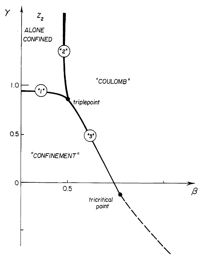
Fig. 1: The phase diagram for $U(1)$ when the two-parameter lattice action is used. This type of action makes it possible to provoke the confinement $Z_{2}$ (or $Z_{3}$) alone. The diagram shows the existence of a triple (critical) point. From this triple point emanate three phase borders: the phase border ”1” separates the totally confining phase from the phase where only the discrete subgroup $Z_{2}$ is confined; the phase border ”2” separates the latter phase from the totally Coulomb–like phase; and the phase border ”3” separates the totally confining and totally Coulomb–like phases.

Monte Carlo simulations of the lattice U(1)–, SU(2)– and SU(3)– gauge theories [1]-[7] indicate the existence of a triple point on the corresponding phase diagrams. A triple point is a boundary point of three first order phase transitions. Such a triple point is shown in Fig.1, which demonstrates the results of the Monte Carlo simulations of the U(1) gauge theory described by the following lattice action [1]-[3]:

$$S=\sum_{\Box}[\beta\cos{\Theta(\Box)}+\gamma\cos{2\Theta(\Box)}].$$ (1)

Here $\Theta(\Box)$ is a plaquette variable.

In the previous works [8]-[13] the investigation of the phase transition phenomena and in particular, the calculation of the U(1) critical coupling constant were connected with the existence of artifact monopoles in the lattice gauge theory and also in the Wilson loop action model, which we proposed in Ref.[13].

Now, instead of using the lattice or Wilson loop cut-off, we are going to introduce physically existing monopoles into the theory as fundamental fields. This idea was suggested previously in Refs.[14]-[16].

Developing a version of the local field theory of the Higgs scalar monopoles and electrically charged particles, we consider in Section 2 an Abelian gauge theory in the Zwanziger formalism [17]–[20] and look for a/or rather several phase transitions connected with the monopoles forming a condensate in the vacuum. This Zwanziger formalism revealing a dual symmetry contains two vector potentials $A_{\mu}(x)$ and $B_{\mu}(x)$ describing one physical photon. Using such an Abelian gauge theory with both magnetic and electric charges, we confirm in Section 3 rather simple expression for the effective potential in the one-loop approximation which was obtained for the Higgs scalar electrodynamics in Ref.[21] (see also the review [22] and Ref.[23]). Using the renormalization group improvement of this effective potential in Section 4, we investigate in Section 6 the phase structure of the Higgs model with scalar monopoles.

In Section 5 we revise the results of Ref.[20] where the renormalization group equations for the electric and magnetic fine structure constants were obtained in the case of the existence of both charges. The Dirac relation for the renormalized effective coupling constants is considered. The influence of the electric charge on the monopole running fine structure constant is investigated.

In Section 6 we show that the first–order phase transition arises in the Higgs monopole model already on the level of the ”improved” one–loop approximation for the effective potential. We argue for the existence of a triple point in the phase diagram ($\lambda_{run};g^{4}_{run}$), where $\lambda_{run}$ is the renormalized running selfinteraction constant in the Higgs monopole model and $g_{run}$ is the running magnetic charge of monopole. We have obtained the triple point values $(\lambda_{(A)};g^{2}_{(A)})\approx(-13.4;18.6)$ and the critical values of the magnetic fine structure constant $\tilde{\alpha}_{crit}=g^{2}_{(A)}/4\pi\approx{1.48}$ and electric fine structure constant $\alpha_{crit}=\pi/g^{2}_{(A)}\approx{0.17}$ (by the Dirac relation). The last value is very close to the lattice result [3]: $\alpha_{crit}^{lat}\approx{0.20\pm 0.015}$, which corresponds to the phase transition between the ”Coulomb” and confinement phases in the $U(1)$ lattice gauge theory. Thus, if the lattice phase transition coupling roughly coincides with our Coleman–Weinberg model it cannot depend much on lattice details. Then we can expect that an ”approximate universality” (regularization independence) of the critical coupling constants, previously suggested in Refs.[10] and [13], takes place even for the first order phase transitions. But this problem needs further more exact investigations.

Section 7 is devoted to the description of the confinement of the electrically charged particles by ANO ”strings” — electric vortices, which exist in the phase with nonzero monopole Higgs field VEVs.

The results of the present paper are very encouraging for the Multiple Point Model [8]-[16], [24]-[28]. This problem is discussed in Section 8.

2 The Zwanziger Formalism for the Abelian Gauge Theory with Electric and Magnetic Charges. Dual Symmetry

A version of the local field theory of electrically and magnetically charged particles is represented by Zwanziger formalism [17],[18] (see also [19] and [20]), which considers two potentials $A_{\mu}(x)$ and $B_{\mu}(x)$ describing one physical photon with two physical degrees of freedom. Now and below we call this theory QEMD (”Quantum ElectroMagnetoDynamics”).

In QEMD the total field system of the gauge, electrically ($\Psi$) and magnetically ($\Phi$) charged fields (with charges $e$ and $g$, respectively) is described by the partition function which has the following form in Euclidean space:

$$Z=\int[DA][DB][D\Phi][D\Phi^{+}][D\Psi][D\Psi^{+}]e^{-S},$$ (2)

where

$$S=\int d^{4}xL(x)=S_{Zw}(A,B)+S_{gf}+S_{(matter)}.$$ (3)

The Zwanziger action $S_{Zw}(A,B)$ is given by:

$$S_{Zw}(A,B)=\int d^{4}x[\frac{1}{2}{(n\cdot[\partial\wedge A])}^{2}+\frac{1}{2}{(n\cdot[\partial\wedge B])}^{2}+\\$$

$$+\frac{i}{2}(n\cdot[\partial\wedge A])(n\cdot{[\partial\wedge B]}^{*})-\frac{i}{2}(n\cdot[\partial\wedge B])(n\cdot{[\partial\wedge A]}^{*})],$$ (4)

where we have used the following designations:

$${[A\wedge B]}_{\mu\nu}=A_{\mu}B_{\nu}-A_{\nu}B_{\mu},\quad{(n\cdot[A\wedge B])}_{\mu}=n_{\nu}{(A\wedge B)}_{\nu\mu},\\$$

$$\quad{G}^{*}_{\mu\nu}=\frac{1}{2}\epsilon_{\mu\nu\lambda\rho}G_{\lambda\rho}.$$ (5)

In Eqs.(4) and(5) the unit vector $n_{\mu}$ represents the fixed direction of the Dirac string in the 4–space.

The action $S_{(matter)}$:

$$S_{(matter)}=\int d^{4}xL_{(matter)}(x)$$ (6)

describes the electrically and magnetically charged matter fields.

$S_{gf}$ is the gauge–fixing action.

Let us consider now the Lagrangian $L_{(matter)}$ describing the Higgs scalar fields $\Psi(x)$ and $\Phi(x)$ interacting with gauge fields $A_{\mu}(x)$ and $B_{\mu}(x)$, respectively:

$$L_{(matter)}(x)=\frac{1}{2}{|D_{\mu}\Psi|}^{2}+\frac{1}{2}{|{\tilde{D}}_{\mu}\Phi|}^{2}-U(\Psi,\Phi),$$ (7)

where

$$D_{\mu}=\partial_{\mu}-ieA_{\mu},$$ (8)

and

$${\tilde{D}}_{\mu}=\partial_{\mu}-igB_{\mu}$$ (9)

are covariant derivatives;

$$U(\Psi,\Phi)=\frac{1}{2}\mu_{e}^{2}{|\Psi|}^{2}+\frac{\lambda_{e}}{4}{|\Psi|}^{4}+\frac{1}{2}\mu_{m}^{2}{|\Phi|}^{2}+\frac{\lambda_{m}}{4}{|\Phi|}^{4}+\lambda_{1}{|\Psi|}^{2}{|\Phi|}^{2}$$ (10)

is the Higgs potential for the electrically and magnetically charged fields $\Psi$ and $\Phi$.

The complex scalar fields:

$$\Psi=\psi+i\zeta\qquad\mbox{and}\qquad\Phi=\phi+i\chi$$ (11)

contain the Higgs $(\psi,\phi)$ and Goldstone $(\zeta,\chi)$ boson fields.

The gauge–fixed action chosen in Ref.[19]:

$$S_{gf}=\int d^{4}x[\frac{M^{2}_{A}}{2}{(n\cdot A)}^{2}+\frac{M^{2}_{B}}{2}{(n\cdot B)}^{2}]$$ (12)

has no ghosts.

The interactions in the Lagrangian (7) are given by terms $j_{\mu}^{e}A_{\mu}$ and $j_{\mu}^{m}B_{\mu}$ (here $j_{\mu}^{e}$ and $j_{\mu}^{m}$ are the electric and magnetic currents) as well as by ”sea–gull” terms $e^{2}A_{\mu}^{2}{|\Psi|}^{2}$ and $g^{2}B_{\mu}^{2}{|\Phi|}^{2}$. The local interaction of the electric and magnetic charges is described by the term $\lambda_{1}{|\Psi|}^{2}{|\Phi|}^{2}$ of Eq.(10) and also is carried out via the ”metamorphosic” propagator $<0|A_{\mu}B_{\nu}|0>$ (see Refs.[19],[20]).

Letting

$$F=\partial\wedge A=-(\partial\wedge B)^{*},$$ (13)

$$F^{*}=\partial\wedge B=(\partial\wedge A)^{*},$$ (14)

and the Hodge star operation (5) on the field tensor:

$$F_{\mu\nu}^{*}=\frac{1}{2}\epsilon_{\mu\nu\rho\sigma}F_{\rho\sigma},$$ (15)

it is easy to see that the free Zwanziger Lagrangian (4) is invariant under the following duality transformations:

$$F\leftrightarrow F^{*},\quad\quad(\partial\wedge A)\leftrightarrow(\partial\wedge B),\quad\quad(\partial\wedge A)^{*}\leftrightarrow-(\partial\wedge B)^{*}.$$ (16)

The Lorentz invariance is lost in the Zwanziger Lagrangian (4) because of depending on a fixed vector $n_{\mu}$, but this invariance is regained for the quantized values of coupling constants $e$ and $g$ obeying the Dirac relation:

$$e_{i}g_{j}=2\pi n_{ij},~{}~{}~{}~{}~{}n_{ij}\in Z.$$ (17)

We also have a dual symmetry as the invariance of the total Lagrangian $L(x)$ under the exchange of the electric and magnetic fields (the Hodge star duality) provided that at the same time the electric and magnetic charges and currents transform according to the following discrete dual symmetry:

$$e\rightarrow g,\qquad g\rightarrow-e,$$

$$\qquad j_{\mu}^{e}\rightarrow j_{\mu}^{m},\qquad j_{\mu}^{m}\rightarrow-j_{\mu}^{e}.$$ (18)

The masses and selfinteraction constants $\lambda_{e,m}$ of the electrically and magnetically charged particles are also interchanged (if they are different):

$$\mu_{e}\leftrightarrow\mu_{m},\qquad\lambda_{e}\leftrightarrow\lambda_{m}.$$ (19)

Considering the electric and magnetic fine structure constants:

$\alpha=\frac{e^{2}}{4\pi}$  and  $\tilde{\alpha}=\frac{g^{2}}{4\pi}$ ,

we have the invariance of the QEMD under the interchange

$$\alpha\leftrightarrow\tilde{\alpha}.$$ (20)

The case $n_{ij}=1$ corresponds to the Dirac relation for elementary charges:

$$eg=2\pi,$$ (21)

which can be rewritten in the following form:

$$\alpha\tilde{\alpha}=\frac{1}{4},$$ (22)

Then we elicit a fact of the invariance of the QEMD under the interchange:

$$\alpha\leftrightarrow\frac{1}{4\alpha}.$$ (23)

Such a dual symmetry follows from Eq.(18). Now we are ready to calculate the effective potential.

3 The Coleman–Weinberg Effective Potential for the Higgs Model with Electrically and Magnetically Charged Scalar Fields

The effective potential in the Higgs model of electrodynamics for a charged scalar field was calculated in the one-loop approximation for the first time by the authors of Ref.[21]. The general method of the calculation of the effective potential is given in the review [22]. Using this method we can construct the effective potential (also in the one–loop approximation) for the theory described by the partition function (2) with the action $S$, containing the Zwanziger action (4), gauge fixing action (12) and the action (7) for the electrically and magnetically charged matter fields.

Let us consider now the shifts:

$$\Psi=\Psi_{B}+{\hat{\Psi}}(x),\quad\quad\Phi(x)=\Phi_{B}+{\hat{\Phi}}(x)$$ (24)

with $\Psi_{B}$ and $\Phi_{B}$ as background fields and calculate the following expression for the partition function in the one-loop approximation:

$$Z=\int[DA][DB][D\hat{\Phi}][D{\hat{\Phi}}^{+}][D\hat{\Psi}][D{\hat{\Psi}}^{+}]\times\\$$

$$\exp\{-S(A,B,\Phi_{B},\Psi_{B})-\int d^{4}x[\frac{\delta S(\Phi)}{\delta\Phi(x)}|_{\Phi=\Phi_{B}}{\hat{\Phi}}(x)+\frac{\delta S(\Psi)}{\delta\Psi(x)}|_{\Psi=\Psi_{B}}{\hat{\Psi}}(x)+h.c.]\}\\$$

$$=\exp\{-F(\Psi_{B},\Phi_{B},e^{2},g^{2},\mu_{e}^{2},\mu_{m}^{2},\lambda_{e},\lambda_{m})\}.$$ (25)

Using the representations (11), we obtain the effective potential:

$$V_{eff}=F(\psi_{B},\phi_{B},e^{2},g^{2},\mu_{e}^{2},\mu_{m}^{2},\lambda_{e},\lambda_{m})$$ (26)

given by the function $F$ of Eq.(25) for the constant background fields:

$$\Psi_{B}=\psi_{B}=\mbox{const},\qquad\qquad\Phi_{B}=\phi_{B}=\mbox{const}.$$ (27)

The effective potential (26) has several minima. Their position depends on $e^{2},g^{2},\mu^{2}_{e,m}$ and $\lambda_{e,m}$. If the first local minimum occurs at $\psi_{B}=0$ and $\phi_{B}=0$, it corresponds to the so-called ”symmetrical phase”, which is the Coulomb-like phase in our description.

We are interested in the phase transition from the Coulomb-like phase ”$\psi_{B}=\phi_{B}=0$” to the confinement phase ”$\psi_{B}=0,\;\phi_{B}=\phi_{0}\neq 0$”. In this case the one–loop effective potential for monopoles coincides with the expression of the effective potential calculated by authors of Ref.[21] for scalar electrodynamics and extended to the massive theory in Ref.[23] (see review [22]):

$$V_{eff}(\phi_{B}^{2})=\frac{\mu_{m}^{2}}{2}{\phi_{B}}^{2}+\frac{\lambda_{m}}{4}{\phi_{B}}^{4}$$

$$+\frac{1}{64\pi^{2}}[3g^{4}{\phi_{B}}^{4}\log\frac{\phi_{B}^{2}}{M^{2}}+{(\mu_{m}^{2}+3\lambda_{m}{\phi_{B}}^{2})}^{2}\log\frac{\mu_{m}^{2}+3\lambda_{m}\phi_{B}^{2}}{M^{2}}$$

$$+{(\mu_{m}^{2}+\lambda_{m}\phi_{B}^{2})}^{2}\log\frac{\mu_{m}^{2}+\lambda_{m}\phi_{B}^{2}}{M^{2}}]+C,$$ (28)

where $M$ is the cut–off scale and C is a constant not depending on $\phi_{B}^{2}$.

Considering the existence of the first vacuum at $\phi_{B}=0$, we have $V_{eff}(0)=0$ and it is easy to determine the constant C:

$$C=-\frac{\mu_{m}^{4}}{16{\pi^{2}}}\log\frac{\mu_{m}}{M}.$$ (29)

Using from now the designations:$\quad\mu=\mu_{m},\quad\lambda=\lambda_{m}$, we have the effective potential in the Higgs monopole model described by the following expression equivalent to Eq.(28):

$$V_{eff}(\phi^{2})=\frac{\mu^{2}_{run}}{2}\phi_{B}^{2}+\frac{\lambda_{run}}{4}\phi_{B}^{4}+\frac{\mu^{4}}{64\pi^{2}}\log\frac{(\mu^{2}+3\lambda\phi_{B}^{2})(\mu^{2}+\lambda\phi_{B}^{2})}{\mu^{4}}.$$ (30)

Here $\lambda_{run}$ is the running self–interaction constant given by the expression standing before $\phi_{B}^{4}$ in Eq.(28):

$$\lambda_{run}(\phi_{B}^{2})=\lambda+\frac{1}{16\pi^{2}}[3g^{4}\log\frac{\phi_{B}^{2}}{M^{2}}+9{\lambda}^{2}\log\frac{\mu^{2}+3\lambda\phi_{B}^{2}}{M^{2}}+{\lambda}^{2}\log\frac{\mu^{2}+\lambda\phi_{B}^{2}}{M^{2}}].$$ (31)

The running squared mass of Higgs scalar monopoles also follows from Eq.(28):

$$\mu^{2}_{run}(\phi_{B}^{2})=\mu^{2}+\frac{\lambda\mu^{2}}{16\pi^{2}}[3\log\frac{\mu^{2}+3\lambda\phi_{B}^{2}}{M^{2}}+\log\frac{\mu^{2}+\lambda\phi_{B}^{2}}{M^{2}}].$$ (32)

As it was shown in Ref.[21], the one–loop effective potential (30) can be improved by the consideration of the renormalization group equation.

4 The Renormalization Group Equation for the Improved Effective Potential

The renormalization group (RG) describes the dependence of a theory and its couplings on an arbitrary scale parameter M. We are interested in RG applied to the effective potential. In this case, knowing the dependence on $M^{2}$ is equivalent to knowing the dependence on $\phi^{2}\equiv\phi_{B}^{2}$. This dependence is given by the renormalization group equations (RGE). Considering the RG improvement of the effective potential, we will follow the approach of Coleman and Weinberg [21] and its extension to the massive theory [23], which are successively described in the review [22]. According to Refs.[21]-[23], RGE for the improved one–loop effective potential is given by the following expression:

$$(M^{2}\frac{\partial}{\partial M^{2}}+\beta_{\lambda}\frac{\partial}{\partial\lambda}+\beta_{g}\frac{\partial}{\partial g}+\beta_{(\mu^{2})}{\mu^{2}}\frac{\partial}{\partial\mu^{2}}-\gamma\phi^{2}\frac{\partial}{\partial\phi^{2}})V_{eff}(\phi^{2})=0,$$ (33)

where the function $\gamma$ is the anomalous dimension:

$$\gamma(\frac{\phi}{M})=-\frac{\partial\phi}{\partial M}.$$ (34)

RGE (33) leads to a new improved effective potential (see the method of its obtaining in the review [22]):

$$V_{eff}(\phi^{2})=\frac{1}{2}\mu^{2}_{run}(t)G^{2}(t)\phi^{2}+\frac{1}{4}\lambda_{run}(t)G^{4}(t)\phi^{4},$$ (35)

where

$$G(t)\equiv\exp[-\frac{1}{2}\int_{0}^{t}dt^{\prime}\gamma\biggl{(}g_{run}(t^{\prime}),\lambda_{run}(t^{\prime})\biggl{)}].$$ (36)

Eq.(33) reproduces also a set of ordinary differential equations:

$$\frac{d\lambda_{run}}{dt}=\beta_{\lambda}\biggl{(}g_{run}(t),\lambda_{run}(t)\biggl{)},$$ (37)

$$\frac{d\mu^{2}_{run}}{dt}=\mu^{2}_{run}(t)\beta_{(\mu^{2})}\biggl{(}g_{run}(t),\lambda_{run}(t)\biggl{)},$$ (38)

$$\frac{dg_{run}}{dt}=\beta_{g}\biggl{(}g_{run}(t),\lambda_{run}(t)\biggl{)},$$ (39)

where $t=\log(\phi^{2}/{M^{2}})$.

We can determine both beta functions for $\lambda_{run}$ and $\mu^{2}_{run}$ by considering a change in M in the conventional non–improved one–loop potential given by Eqs.(30), (31) and (32).

Let us write now the one–loop potential (30) as

$$V_{eff}=V_{0}+V_{1},$$ (40)

where

$$V_{0}=\frac{\mu^{2}}{2}\phi^{2}+\frac{\lambda}{4}\phi^{4}$$ (41)

and

$$V_{1}=\frac{1}{64\pi^{2}}[3g^{4}{\phi}^{4}\log\frac{\phi^{2}}{M^{2}}+{(\mu^{2}+3\lambda{\phi}^{2})}^{2}\log\frac{\mu^{2}+3\lambda\phi^{2}}{M^{2}}$$

$$+{(\mu^{2}+\lambda\phi^{2})}^{2}\log\frac{\mu^{2}+\lambda\phi^{2}}{M^{2}}-2\mu^{4}\log\frac{\mu^{2}}{M^{2}}].$$ (42)

We can plug this $V_{eff}$ into RGE (33) and obtain the following equation (see [22]):

$$(\beta_{\lambda}\frac{\partial}{\partial\lambda}+\beta_{(\mu^{2})}{\mu^{2}}\frac{\partial}{\partial\mu^{2}}-\gamma\phi^{2}\frac{\partial}{\partial\phi^{2}})V_{0}=-M^{2}\frac{\partial V_{1}}{\partial M^{2}}.$$ (43)

Equating $\phi^{2}$ and $\phi^{4}$ coefficients, we obtain:

$$\beta_{\lambda}=2\gamma\lambda_{run}+\frac{5\lambda_{run}^{2}}{8\pi^{2}}+\frac{3g_{run}^{4}}{16\pi^{2}},$$ (44)

$$\beta_{(\mu^{2})}=\gamma+\frac{\lambda_{run}}{4\pi^{2}}.$$ (45)

The result for $\gamma$ is given in Ref.[21] for scalar field with electric charge $e$, but it is easy to rewrite this $\gamma$–expression for monopoles with charge $g=g_{run}$:

$$\gamma=-\frac{3g_{run}^{2}}{16\pi^{2}}.$$ (46)

Finally we have:

$$\frac{d\lambda_{run}}{dt}=\frac{1}{16\pi^{2}}(3g^{4}_{run}+10\lambda^{2}_{run}-6\lambda_{run}g^{2}_{run}),$$ (47)

$$\frac{d\mu^{2}_{run}}{dt}=\frac{\mu^{2}_{run}}{16\pi^{2}}(4\lambda_{run}-3g^{2}_{run}).$$ (48)

Now the aim is to calculate the $\beta_{g}$–function, and here, as it was shown in the next Section, we have the difference between the scalar electrodynamics [21] and scalar QEMD.

5 Renormalization Group Equation for the Magnetic Charge. The Dirac Relation

It is well-known that in the absence of monopoles the Gell–Mann–Low equation has the following form:

$$\frac{\mbox{d}(\log\alpha(p))}{\mbox{d}t}=\beta(\alpha(p)),$$ (49)

where $t=\log(p^{2}/M^{2})$, $p$ is a 4-momentum and $\alpha=e^{2}/4\pi$. Let us consider also an energy scale $\tilde{\mu}$: $p^{2}={\tilde{\mu}}^{2}$ and $t=2\log(\tilde{\mu}/M)$.

As it was first shown in Refs.[29], at sufficiently small charge ($\alpha<1$) the $\beta-$function is given by series over $\alpha/4\pi$:

$$\beta(\alpha)=\beta_{2}(\frac{\alpha}{4\pi})+\beta_{4}{(\frac{\alpha}{4\pi})}^{2}+...$$ (50)

The first two terms of this series were calculated in the QED long time ago in Refs.[29],[30]. The following result was obtained in the framework of perturbation theory (in the one- and two-loop approximations):

a)

$$\beta_{2}=\frac{4}{3}\quad\mbox{and}\quad\beta_{4}=4\quad-\quad\mbox{for fermion (electron) loops},$$ (51)

and

b)

$$\beta_{2}=\frac{1}{3}\quad\mbox{and}\quad\beta_{4}=1\quad-\quad\mbox{for scalar particle loops}.$$ (52)

This result means that for scalar particles the $\beta$-function can be represented by the following series aroused from Eq.(50):

$$\beta(\alpha)=\frac{\alpha}{12\pi}(1+3\frac{\alpha}{4\pi}+...)$$ (53)

and we are able to exploit the one-loop approximation (given by the first term of Eqs.(50) and (53)) up to $\alpha\sim 1$ (with accuracy $\approx 25\%$ for $\alpha\simeq 1$).

The Dirac relation and the renormalization group equations (RGE) for the electric and magnetic fine structure constants $\alpha$ and $\tilde{\alpha}$ were investigated in detail by the authors in their recent paper [26], where the same Zwanziger formalism was developed for the QEMD. The following result was obtained.

If we have the electrically and magnetically charged particles existing simultaneously for $\tilde{\mu}>\tilde{\mu}_{(threshold)}$ and if in some region of $\tilde{\mu}$ their Gell–Mann–Low $\beta$–functions are computable perturbatively as a power series in $e^{2}$ and $g^{2}$, then the Dirac relation [31] is valid not only for the ”bare” elementary charges $e_{0}$ and $g_{0}$, but also for the renormalized effective charges $e$ and $g$ (see the history of this problem in Refs.[32] and in the review [33]):

$$eg=e_{0}g_{0}=2\pi.$$ (54)

Then

$$\alpha(t)\tilde{\alpha}(t)=\frac{1}{4}\qquad{\mbox{for any}}\quad\tilde{\mu}~{}\geq~{}\tilde{\mu}_{\mbox{(threshold)}}.$$ (55)

Eq.(55) confirms the equality:

$$\frac{d\log\alpha(p)}{dt}=-\frac{d\log\tilde{\alpha}(p)}{dt}$$ (56)

in the corresponding region of $t$.

Now if there exists a region of $\alpha$ and $\tilde{\alpha}$, where we can describe monopoles and electrically charged scalar particles by a perturbation theory, then the following RG–equations (obtained in [20]) take place:

$$\frac{d\log\alpha(p)}{dt}=-\frac{d\log{\tilde{\alpha}}(p)}{dt}=\beta^{(e)}(\alpha)-\beta^{(m)}(\tilde{\alpha}).$$ (57)

These RGE are in accordance not only with the Dirac relation (55), but also with the dual symmetry considered in Section 2.

If both $\alpha$ and $\tilde{\alpha}$ are sufficiently small, then the functions $\beta^{(e,m)}$ in Eq.(57) are described by the contributions of the electrically and magnetically charged particle loops [20]. Their analytical expressions are given by the usual series similar to (50). By restricting ourselves to the two–loop approximation, we have the following equations (57) for scalar particles:

$$\frac{d\log\alpha(p)}{dt}=-\frac{d\log{\tilde{\alpha}}(p)}{dt}=\frac{\alpha-\tilde{\alpha}}{12\pi}(1+3\frac{\alpha+\tilde{\alpha}}{4\pi}+....).$$ (58)

It is not difficult to see that $\beta^{(e,m)}$ coincide with the usual well–known $\beta$–functions calculated in QED only in the two–loop approximation. The deviation from the QED expressions for $\beta$–functions arises only on the level of the higher order approximations when the monopole (or electric particle) loops begin to play a role in the electric (or monopole) loops.

According to Eq.(58), the two–loop contribution is not more than $30\%$ if both $\alpha$ and $\tilde{\alpha}$ obey the following requirement:

$$0.25\stackrel{{\scriptstyle<}}{{\sim}}{\large\alpha,\tilde{\alpha}}\stackrel{{\scriptstyle<}}{{\sim}}1.$$ (59)

The lattice simulations of compact QED give the behavior of the effective fine structure constant $\alpha(\beta)$ ($\beta=1/e_{0}^{2}$ in Eq.(116), and $e_{0}$ is the bare electric charge) in the vicinity of the phase transition point (see Refs.[2],[3],[5]). The following critical value of the fine structure constant $\alpha$ was obtained in Ref.[3]:

$$\alpha_{crit}^{lat}\approx{0.20\pm 0.015}\quad\quad\mbox{at}\quad\quad\beta_{crit}\approx{1.011}.$$ (60)

By the Dirac relation (55), it is easy to obtain the corresponding critical value of the monopole fine structure constant:

$${\tilde{\alpha}}_{crit}^{lat}\approx{1.25\pm 0.10}.$$ (61)

These lattice critical values of the fine structure constants $\alpha$ and $\tilde{\alpha}$ correspond to the phase transition point $(\beta,\gamma)\approx(1,0)$ belonging to the phase diagram presented in Fig.1.

Eqs.(60) and (61) demonstrate that $\alpha$ and $\tilde{\alpha}\;$ considered in the compact (lattice) QED in the vicinity of the phase transition point almost coincide with the borders of the requirement (59) given by the perturbation theory for $\beta$–functions.

Assuming that in the vicinity of the phase transition point the coupling constant $g_{run}$ may be described by the one–loop approximation, we obtain from Eq.(58) the following RGE for $g_{run}^{2}$:

$$\frac{d\log(g_{run}^{2})}{dt}=\frac{g^{2}_{run}-e^{2}_{run}}{48\pi^{2}}.$$ (62)

Using the Dirac relation (55), we have:

$$\frac{dg^{2}_{run}}{dt}=\frac{g^{4}_{run}}{48\pi^{2}}-\frac{1}{12}.$$ (63)

Note that the second term of Eq.(63) describes the influence of the electrically charged fields on the behavior of the monopole charge. In the case $\tilde{\alpha}>>\alpha$ we can neglect the second term on the right side of Eq.(63). Then we have the usual running coupling in the dual sector of the scalar electrodynamics, which according to Eq.(58), is given by the following RGE in the two–loop approximation:

$$\frac{dg^{2}_{run}}{dt}=\frac{g^{4}_{run}}{48\pi^{2}}+\frac{g^{6}_{run}}{{(16\pi^{2})}^{2}}.$$ (64)

These expressions of RGE for $g^{2}_{run}$ will be exploited in the next Section for the investigation of the phase transition couplings in our model.

6 Calculation of the Triple Point Couplings in the Higgs Monopole Model of U(1) Gauge Theory

As it was mentioned in Section 3, we consider the phase transition from the Coulomb–like phase ”$\psi_{B}=\phi_{B}=0$” to the phase with ”$\psi_{B}=0,\;\phi_{B}=\phi_{0}\neq 0$”. This means that the effective potential (35) of the Higgs scalar monopoles has the first and the second minima appearing at $\phi=0$ and $\phi=\phi_{0}$, respectively. They are shown in Fig.2 by the curve ”1”. These minima of $V_{eff}(\phi^{2})$ correspond to the different vacua arising in the model. The conditions for the existence of degenerate vacua are given by the following equations:

$$V_{eff}(0)=V_{eff}(\phi_{0}^{2})=0,$$ (65)

$$\frac{\partial V_{eff}}{\partial\phi}|_{\phi=0}=\frac{\partial V_{eff}}{\partial\phi}|_{\phi=\phi_{0}}=0$$ (66)

with inequalities

$$\frac{\partial^{2}V_{eff}}{\partial\phi^{2}}|_{\phi=0}>0,\quad\frac{\partial^{2}V_{eff}}{\partial\phi^{2}}|_{\phi=\phi_{0}}>0.$$ (67)

The $\phi=\phi_{0}$ equation and inequality here are equivalent to:

$$V^{\prime}_{eff}(\phi_{0}^{2})\equiv\frac{\partial V_{eff}}{\partial\phi^{2}}|_{\phi=\phi_{0}}=0,$$ (68)

$$V^{\prime\prime}_{eff}(\phi_{0}^{2})\equiv\frac{\partial^{2}V_{eff}}{\partial{(\phi^{2})}^{2}}|_{\phi=\phi_{0}}>0$$ (69)

using $\phi^{2}$ as variable. The first equation (65) applied to Eq.(35) gives:

$$\mu_{run}^{2}=-\frac{1}{2}\lambda_{run}(t_{0}){\phi_{0}^{2}}G^{2}(t_{0}),$$ (70)

where $t_{0}=\log(\phi_{0}^{2}/M^{2})$.

The calculation of the first derivative of $V_{eff}(\phi^{2})$ leads to the following expression:

$$V^{\prime}_{eff}(\phi^{2})=\frac{V_{eff}(\phi^{2})}{\phi^{2}}(1+2\frac{d\log G}{dt})+\frac{1}{2}\frac{d\mu^{2}_{run}}{dt}G^{2}(t)$$

$$+\frac{1}{4}\biggl{(}\lambda_{run}(t)+\frac{d\lambda_{run}}{dt}+2\lambda_{run}\frac{d\log G}{dt}\biggr{)}G^{4}(t)\phi^{2}.$$ (71)

From Eq.(36) and (46) we have:

$$\frac{d\log G}{dt}=-\frac{1}{2}\gamma=\frac{3g^{2}_{run}}{32\pi^{2}}.$$ (72)

Using Eqs.(47), (48), (70) and (72), it is easy to find the joint solution of equations $V_{eff}(\phi_{0}^{2})=V^{\prime}_{eff}(\phi_{0}^{2})=0$:

$${V^{\prime}}_{eff}(\phi_{0}^{2})=(\frac{3}{16\pi^{2}}g^{4}_{run}+\lambda_{run}+\frac{3}{8}\frac{{\lambda_{run}}^{2}}{\pi^{2}})G^{4}(t_{0})\phi_{0}^{2}=0,$$ (73)

or

$$g^{4}_{crit}=-2\lambda_{run}(\frac{8\pi^{2}}{3}+\lambda_{run}).$$ (74)

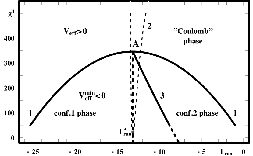
Fig. 3: The phase diagram ($\lambda_{run};\;{\rm g}^{4}\equiv g^{4}_{run}$) corresponding to the Higgs monopole model shows the existence of a triple point A $\bigl{(}\lambda_{(A)}\approx-13.4;\;{\rm g}^{2}_{(A)}\approx 18.6\bigr{)}$. This triple point is a boundary point of three phase transitions: the ”Coulomb-like” phase and two confinement phases (”conf.1” and ”conf.2”) meet together at the triple point A. The dashed curve ”2” shows the requirement: $V_{eff}(\phi_{0}^{2})=V^{\prime\prime}_{eff}(\phi_{0}^{2})=0$. Monopole condensation leads to the confinement of the electric charges: ANO electric vortices (with electric charges at their ends, or closed) are created in the confinement phases ”conf.1” and ”conf.2”.

The curve (74) is represented on the phase diagram $(\lambda_{run};g^{4}_{run})$ of Fig.3 by the curve ”1” which describes a border between the ”Coulomb–like” phase with $V_{eff}\geq 0$ and the confinement ones having $V_{eff}^{min}<0$.

The next step is the calculation of the second derivative of the effective potential:

$${V^{\prime\prime}}_{eff}(\phi^{2})=\frac{{V^{\prime}}_{eff}(\phi^{2})}{\phi^{2}}+\biggl{(}-\frac{1}{2}\mu^{2}_{run}+\frac{1}{2}\frac{d^{2}\mu^{2}_{run}}{dt^{2}}+2\frac{d\mu^{2}_{run}}{dt}\frac{d\log G}{dt}$$

$$+\mu^{2}_{run}\frac{d^{2}\log G}{dt^{2}}+2\mu^{2}_{run}{(\frac{d\log G}{dt})}^{2}\biggl{)}\frac{G^{2}}{\phi^{2}}+\biggl{(}\frac{1}{2}\frac{d\lambda_{run}}{dt}+\frac{1}{4}\frac{d^{2}\lambda_{run}}{dt^{2}}+2\frac{d\lambda_{run}}{dt}\frac{d\log G}{dt}$$

$$+2\lambda_{run}\frac{d\log G}{dt}+\lambda_{run}\frac{d^{2}\log G}{dt^{2}}+4\lambda_{run}{(\frac{d\log G}{dt})}^{2}\biggl{)}G^{4}(t).$$ (75)

Let us consider now the case when this second derivative changes its sign giving a maximum of $V_{eff}$ instead of the minimum at $\phi^{2}=\phi_{0}^{2}$. Such a possibility is shown in Fig.2 by the dashed curve ”2”.

Now two additional minima at $\phi^{2}=\phi_{1}^{2}$ and $\phi^{2}=\phi_{2}^{2}$ appear in our theory. They correspond to two different confinement phases related with the confinement of the electrically charged particles. If these two minima are degenerate, then we have the following requirements:

$$V_{eff}(\phi_{1}^{2})=V_{eff}(\phi_{2}^{2})<0$$ (76)

and

$${V^{\prime}}_{eff}(\phi_{1}^{2})={V^{\prime}}_{eff}(\phi_{2}^{2})=0,$$ (77)

which describe the border between the confinement phases ”conf.1” and ”conf.2” presented in Fig.3. This border is given as a curve ”3” at the phase diagram $(\lambda_{run};g^{4}_{run})$ drawn in Fig.3. The curve ”3” meets the curve ”1” at the triple point A (see Fig.3). According to the illustration shown in Fig.2, it is obvious that this triple point A is given by the following requirements:

$$V_{eff}(\phi_{0}^{2})=V^{\prime}_{eff}(\phi_{0}^{2})=V^{\prime\prime}_{eff}(\phi_{0}^{2})=0.$$ (78)

In contrast to the requirements:

$$V_{eff}(\phi_{0}^{2})=V^{\prime}_{eff}(\phi_{0}^{2})=0,$$ (79)

giving the curve ”1”, let us consider now the joint solution of the following equations:

$$V_{eff}(\phi_{0}^{2})=V^{\prime\prime}_{eff}(\phi_{0}^{2})=0.$$ (80)

It is easy to obtain this solution using Eqs.(75), (70), (47), (48) and (63):

$${\cal F}(\lambda_{run},g^{2}_{run})-\pi^{2}(\lambda_{run}-2g^{2}_{run})=0,$$ (81)

where

$${\cal F}(\lambda_{run},g^{2}_{run})=5g_{run}^{6}+24\pi^{2}g_{run}^{4}+12\lambda_{run}g_{run}^{4}-9\lambda_{run}^{2}g_{run}^{2}$$

$$+36\lambda_{run}^{3}+80\pi^{2}\lambda_{run}^{2}+64\pi^{4}\lambda_{run}.$$ (82)

The dashed curve ”2” of Fig.3 represents the solution of Eq.(81) which is equivalent to Eqs.(80). The curve ”2” is going very close to the maximum of the curve ”1”. It is natural to assume that the position of the triple point A coincides with this maximum and the corresponding deviation can be explained by our approximate calculations. Taking into account such an assumption, let us consider the border between the phase ”conf.1” having the first minimum at nonzero $\phi_{0}$ with $V_{eff}^{min}=c_{1}<0$ and the phase ”conf.2 ” which reveals two minima with the second minimum being the deeper one and having $V_{eff}^{min}=c_{2}<0$. This border (described by the curve ”3” of Fig.3) was calculated in the vicinity of the triple point A by means of Eqs.(76) and (77) with $\phi_{1}$ and $\phi_{2}$ represented as $\phi_{1,2}=\phi_{0}\pm\epsilon$ with $\epsilon<<\phi_{0}$. The result of such calculations gives the following expression for the curve ”3”:

$$g^{4}_{run}=\frac{5}{2}(5\lambda_{run}+8\pi^{2})\lambda_{run}+8\pi^{4}.$$ (83)

The curve ”3” meets the curve ”1” at the triple point A.

The piece of the curve ”1” to the left of the point A describes the border between the ”Coulomb–like” phase and the phase ”conf.1”. In the vicinity of the triple point A the second derivative $V_{eff}^{\prime\prime}(\phi_{0}^{2})$ changes its sign leading to the existence of the maximum at $\phi^{2}=\phi_{0}^{2}$, in correspondence with the dashed curve ”2” of Fig.2. By this reason, the curve ”1” does not already describe a phase transition border up to the next point B when the curve ”2” again intersects the curve ”1” at $\lambda_{(B)}\approx-12.24$. This intersection (again giving $V^{\prime\prime}_{eff}(\phi_{0}^{2})>0$) occurs supprisingly quickly.

The right piece of the curve ”1” along to the right of the point B separates the ”Coulomb” phase and the phase ”conf.2”. But between the points A and B the phase transition border is going slightly upper the curve ”1”. This deviation is very small and can’t be distinguished on Fig.3.

The joint solution of equations (78) leads to the joint solution of Eqs.(74) and (81).

It is necessary to note that only $V^{\prime\prime}_{eff}(\phi^{2})$ contains the derivative $dg^{2}_{run}/dt$. According to Eqs.(62) and (63), the influence of the electric charge is described by the second term of Eq.(81).

With aim to investigate a position of the triple point, let us consider the joint solution of Eqs.(78) in the following three cases:

a) The joint solution of Eqs.(74) and

$${\cal F}(\lambda_{run},g^{2}_{run})=0$$ (84)

neglects the influence of the electrically charged fields.

b) The joint solution of Eqs.(74) and (81) takes into account the electric charge influence.

c) In the two–loop approximation for $dg^{2}_{run}/dt\;$ and in the absence of the electric charge influence (see RGE (64)), it is necessary to consider the joint solution of Eq.(74) and the following equation:

$${\cal F}(\lambda_{run},g^{2}_{run})+\frac{3}{32\pi^{2}}g^{8}=0.$$ (85)

These solutions were obtained numerically and gave the following triple point values of $\lambda_{run}$ and $g^{2}_{run}$:

$$a)\qquad\lambda_{(A)}\approx{-13.4073},\quad g^{2}_{(A)}\approx{18.6070};$$ (86)

$$b)\qquad\lambda_{(A)}\approx{-13.3696},\quad g^{2}_{(A)}\approx{18.6079};$$ (87)

$$c)\qquad\lambda_{(A)}\approx{-13.4923},\quad g^{2}_{(A)}\approx{18.6044}.$$ (88)

Such results show that the triple point position ($\lambda_{(A)};g^{2}_{(A)})$ is independent of the electric charge influence and two–loop corrections to $dg^{2}_{run}/dt$ with accuracy of deviations $<1\%$.

The numerical solution also demonstrates that the triple point A exists in the very neighborhood of the maximum of the curve (74) and its position is approximately given by the following values:

$$\lambda_{(A)}\approx-\frac{4\pi^{2}}{3}\approx-13.4,$$ (89)

$$g^{2}_{(A)}=g^{2}_{crit}|_{\mbox{for}\;\lambda_{run}=\lambda_{(A)}}\approx\frac{4\sqrt{2}}{3}{\pi^{2}}\approx 18.6.$$ (90)

Let us conclude now what description of the phase diagram shown in Fig.3 we have finally.

There exists three phases in the dual sector of the Higgs scalar electrodynamics : ”Coulomb–like phase” and the confinement phases ”conf.1” and ”conf.2”. The border ”1”, which is described by the curve (74), separates the ”Coulomb–like phase” ($V_{eff}\geq 0$) and the confinement phases ($V_{eff}^{min}(\phi_{0}^{2})<0,\;V^{\prime}_{eff}(\phi_{0}^{2})=0$). The curve ”1” corresponds to the joint solution of the equations $V_{eff}(\phi_{0}^{2})=V^{\prime}_{eff}(\phi_{0}^{2})=0$ in the case b).

The dashed curve ”2” represents the solution of the equations $V_{eff}(\phi_{0}^{2})=V^{\prime\prime}_{eff}(\phi_{0}^{2})=0$.

The phase border ”3” of Fig.3 separates two confinement phases. The following requirements take place for this border:

$$V_{eff}(\phi_{1,2}^{2})<0,\qquad$$

$$V_{eff}(\phi_{1}^{2})=V_{eff}(\phi_{2}^{2}),$$

$$V^{\prime}_{eff}(\phi_{1}^{2})=V^{\prime}_{eff}(\phi_{2}^{2})=0,$$

$$V^{\prime\prime}_{eff}(0)>0,\qquad V^{\prime\prime}_{eff}(\phi_{2}^{2})>0.$$ (91)

The triple point A is a boundary point of all three phase transitions shown in the phase diagram of Fig.3. For $g^{2}<g^{2}_{({A})}$ the field system described by our model exists in the confinement phase, where all electric charges are confined.

The triple point value of the magnetic fine structure constant follows from Eq.(90):

$$\tilde{\alpha}_{(A)}=\frac{g^{2}_{(A)}}{4\pi}\approx 1.48.$$ (92)

By the Dirac relation (55), we have calculated the value of the triple point electric fine structure constant:

$$\alpha_{(A)}=\frac{\pi}{g^{2}_{(A)}}\approx{0.17}.$$ (93)

The obtained result is very close to the Monte Carlo lattice result (60). Taking into account that monopole mass $m$ is given by the following expression:

$$V^{\prime\prime}_{eff}(\phi_{0}^{2})=\frac{1}{2\phi_{0}^{2}}\frac{d^{2}V_{eff}}{d\phi^{2}}|_{\phi=\phi_{0}}=\frac{m^{2}}{2\phi_{0}^{2}},$$ (94)

we see that monopoles acquire zero mass in the vicinity of the triple point A:

$$V^{\prime\prime}_{eff}(\phi_{0A}^{2})=\frac{m^{2}_{(A)}}{2\phi_{0A}^{2}}=0,$$ (95)

and we can compare the values (92) and (93) with the corresponding results obtained in Refs.[5,6] for the compact QED described by the Villain action:

$$\alpha\approx 0.1836,\quad\tilde{\alpha}\approx 1.36,\quad m^{2}\approx 0\quad-\quad\mbox{in the vicinity of the critical point}.$$ (96)

The phase diagram drawn in Fig.3 corresponds to the following region of parameters:

$$0.17\stackrel{{\scriptstyle<}}{{\sim}}{\large\alpha,\tilde{\alpha}}\stackrel{{\scriptstyle<}}{{\sim}}1.5,$$ (97)

where this diagram can be described by the one–loop (renormalization group improved) effective potential. According to Eq.(58), in the region (97) the contribution of two loops is given by the accuracy of deviations not more than $30\%$, therefore the perturbation theory works in this region.

It is necessary to note that the estimation of $\beta_{\lambda}(\lambda,g^{2})$ in RGE (37) indicates a slow convergence of the series over $\lambda$. The comparison of the expressions for the effective potentials $V_{eff}^{(1)}$ and $V_{eff}^{(2)}$ corresponding to the one–loop and two–loop approximations in $\lambda$, respectively, leads to the following relation:

$$V_{eff}^{(2)}\approx V_{eff}^{(1)}(1+\frac{a\lambda_{run}}{48\pi^{2}}+...)$$ (98)

with $a\sim 1$. Such a result allows to consider the one–loop approximation for $\lambda_{run}$ up to $|\lambda|\stackrel{{\scriptstyle<}}{{\sim}}30$ with accuracy of deviations $<10\%$, and the value $\lambda_{(A)}\approx-13$ obtained in the present paper for the triple point A is expected as well described by our method. The analysis of such an estimation was performed with help of Refs.[34],[35] applied to our case of the scalar Higgs fields.

7 ”ANO–strings”, or the vortex description of the confinement phases

As it was shown in the previous Section, two regions between the curves ”1”, ”3” and ”3”, ”1”, given by the phase diagram of Fig.3, correspond to the existence of two confinement phases, different in the sense that the phase ”conf.1” is produced by the second minimum, but the phase ”conf.2” corresponds to the third minimum of the effective potential. It is obvious that in our case both phases have nonzero monopole condensate in the minima of the effective potential, when $V_{eff}^{min}(\phi_{1,2}\neq 0)<0$. By this reason, the Abrikosov–Nielsen–Olesen (ANO) electric vortices (see Refs.[36],[37]) may exist in these both phases, which are equivalent in the sense of the ”string” formation. If electric charges are present in a model (they are given in our model by the electrically charged Higgs field $\Psi$), then these charges are placed at the ends of the vortices–”strings” and therefore are confined.

Utilizing the string formulation of our Abelian Higgs Model (AHM), we can use the result of Ref.[38] and consider the partition function:

$$Z_{AHM}=\int DBD\Phi D{\bar{\Phi}}e^{-S_{AHM}(B,\Phi,\bar{\Phi})}$$ (99)

with

$$S_{AHM}(B,\Phi,\bar{\Phi})=\int d^{4}x\{\frac{1}{4}{(\partial\wedge B)}^{2}+\frac{1}{2}{|(\partial-igB)\Phi|}^{2}+\frac{\lambda}{4}{({|\Phi|}^{2}-\Phi_{0}^{2})}^{2}\},$$ (100)

which in the London limit $(\lambda\to\infty)$ can be rewritten in terms of the world–sheet coordinates $X^{\mu}(\sigma)$ of the ANO closed strings:

$$\lim_{\lambda\to\infty}Z_{AHM}=\int_{\delta\Sigma=0}D\Sigma e^{-S(\Sigma)}.$$ (101)

In Eq.(101) we have:

$$S(\Sigma)=\frac{\pi^{2}m_{V}^{2}}{g^{2}}\int d^{2}\sigma d^{2}\sigma^{\prime}\epsilon^{ab}\partial_{a}X^{\mu}(\sigma)\partial_{b}X^{\nu}(\sigma)K[X(\sigma)-X(\sigma^{\prime})]$$

$$\epsilon^{a^{\prime}b^{\prime}}\partial_{a^{\prime}}X^{\mu}(\sigma^{\prime})\partial_{b^{\prime}}X^{\nu}(\sigma^{\prime}),$$ (102)

where $m_{V}^{2}=g^{2}\phi_{0}^{2}$. The kernel $K(x)$ obeys the following equation:

$$(-{\partial}^{2}+m_{V}^{2})K(x)=\delta(x).$$ (103)

As it is well–known [36],[37], in the London’s limit ($\lambda\to\infty$) the Abelian Higgs model, described by the Lagrangian (7)–(10) with $\Psi=0$, gives the formation of the condensate with amplitude $\phi_{0}$ which repels and suppresses the electromagnetic field $F_{\mu\nu}$ almost everywhere, except the region around the vortex lines. In this limit, we have the following London equation:

$${\mbox{r}ot}\;{\vec{j}}^{m}={\delta}^{-2}{\vec{E}},$$ (104)

where ${\vec{j}}^{m}$ is the microscopic current of monopoles, ${\vec{E}}$ is the electric field strength and $\delta$ is the penetration depth. It is clear that ${\delta}^{-1}$ is the photon mass $m_{V}$, generated by the Higgs mechanism. The closed equation for $\vec{E}$ follows from the Maxwell equations and Eq.(104) just in the London’s limit.

In our case $\delta$ is defined by the following relation:

$${\delta}^{-2}\equiv m_{V}^{2}=g^{2}\phi_{0}^{2}.$$ (105)

On the other hand, the field $\phi$ has its own correlation length $\xi$, connected to the mass of the field $\phi$ (”the Higgs mass”):

$$\xi={m_{S}}^{-1},\qquad m_{S}^{2}=\lambda\phi_{0}^{2}.$$ (106)

The London’s limit for our ”dual superconductor of the second kind” corresponds to the following relations:

$$\delta>>\xi,\qquad m_{V}<<m_{S},\qquad g<<\lambda,$$ (107)

and ”the string tension” — the vortex energy per unit length (see Ref.[37]) — for the minimal electric vortex flux $2\pi$, is:

$$\sigma=\frac{2\pi}{g^{2}\delta^{2}}\ln\frac{\delta}{\xi}=2\pi\phi_{0}^{2}\ln\frac{m_{S}}{m_{V}},\qquad{\mbox{where}}\qquad\delta/\xi=\frac{m_{S}}{m_{V}}>>1.$$ (108)

We see that in the London’s limit ANO–theory implies the mass generation of the photons, $m_{V}=1/\delta$, which is much less than the Higgs mass $m_{S}=1/\xi$.

Let us be interested now in the question whether our ”strings” are thin or not. The vortex may be considered as thin, if the distance between the electric charges sitting at its ends, i.e. the string length $L$, is much larger than the penetration length $\delta$:

$$L>>\delta>>\xi.$$ (109)

In the framework of classical calculations, it is not difficult to obtain the mass $M$ and angular momentum $J$ of the rotating ”string”:

$$J=\frac{1}{2\pi\sigma}M^{2},\qquad M=\frac{\pi}{2}\sigma L.$$ (110)

The following relation follows from Eqs.(110):

$$L=2\sqrt{\frac{2J}{\pi\sigma}},$$ (111)

or

$$L=\frac{2g\delta}{\pi}\sqrt{\frac{J}{\ln\frac{m_{S}}{m_{V}}}}.$$ (112)

For $J=1$ we have:

$$\frac{L}{\delta}=\frac{2g}{\pi\sqrt{\ln\frac{m_{S}}{m_{V}}}},$$ (113)

what means that for $m_{S}>>m_{V}$ the length of this ”string” is small and does not obey the requirement (109). It is easy to see from Eq.(112) that in the London’s limit the ”strings” are very thin ($L/\delta>>1$) only for the enormously large angular momenta $J>>1$.

The phase diagram of Fig.3 shows the existence of the confinement phase for $\alpha\geq\alpha_{(A)}\approx 0.17$. This means that the formation of vortices begins at the triple point $\alpha=\alpha_{(A)}$: for $\alpha>\alpha_{(A)}$ we have nonzero $\phi_{0}$ leading to the existence of vortices.

It is necessary to emphasize that this value $\alpha_{(A)}$, as the lattice $\alpha_{crit}$, is sufficiently small and corresponds to the validity of the perturbation theory for $\beta$–functions of RGE.

The lattice investigations show that in the confinement phase $\alpha(\beta)$ increases when $\beta=1/e_{0}^{2}\to 0$ (here $e_{0}$ is the the bare electric charge) and very slowly approaches to its maximal value (see Refs.[2,3]). Such a phenomenon leads to the ”freezing” of the electric fine structure constant at the value $\alpha=\alpha_{max}$ due to the Casimir effect. The authors of Ref.[39] predicted: $\alpha_{max}=\frac{\pi}{12}\approx 0.26$ (see also Ref.[13]).

Let us consider now the region of the confinement values of the magnetic charge $g$ (obtained in this paper):

$$g_{min}\leq g\leq g_{max},$$

$$g_{max}=g_{(A)}\approx{\sqrt{18.6}}\approx 4.3,$$

$$g_{min}=\sqrt{\frac{\pi}{\alpha_{max}}}\approx 3.5.$$ (114)

Then for $m_{S}=10m_{V}$ say we have from Eq.(113) the following estimation of the ”string” length for $J=1$:

$$1.5\stackrel{{\scriptstyle<}}{{\sim}}\frac{L}{\delta}\stackrel{{\scriptstyle<}}{{\sim}}2.$$ (115)

We see that ”low-lying” states of ”strings” correspond to the short and thick vortices.

It is worthwhile mentioning that the confinement of monopoles is described by the non–dual (usual) sector of the Higgs electrodynamics and the Higgs field $\Psi$, having the electric charge, is responsible for this confinement. The corresponding confinement phases for monopoles are absent on the phase diagram of Fig.3. They can be described by the phase diagram ($\lambda^{e}_{run};e^{2}_{run}$). Of course, the dual symmetry predicts that the triple point $e^{2}_{(A)}$ has to be given by the same value (90), i.e. $\alpha_{(A)}\approx 1.48$ and $\tilde{\alpha}_{(A)}\approx 0.17$. The overall phase diagram is three-dimensional and is given by $(\lambda^{m}_{run};\lambda^{e}_{run};g^{2}_{run})$, because $e^{2}_{run}$ and $g^{2}_{run}$ are related by the Dirac charge quantization condition. It is natural to expect that the region of the monopole confinement also stretches from $\tilde{\alpha}={\tilde{\alpha}}_{(A)}\approx 0.17$ up to the value $\tilde{\alpha}={\tilde{\alpha}}_{max}\approx 0.26$.

8 Multiple Point Principle and the Higgs Monopole Model

Most efforts to explain the Standard Model (SM) describing well all experimental results known today are devoted to Grand Unification Theories (GUTs). The supersymmetric extension of the SM consists of taking the SM and adding the corresponding supersymmetric partners [40]. The Minimal Supersymmetric Standard Model (MSSM) shows the possibility of the existence of the grand unification point at $\mu_{GUT}\sim 10^{16}$ GeV [41]. But the absence of supersymmetric particle production at current accelerators and additional constraints arisen from limits on the contributions of virtual supersymmetric particle exchange to a variety of the SM processes indicate that at present there are no unambiguous experimental results requiring the existence of the supersymmetry [42], [43].

Anti–Grand Unification Theory (AGUT) was developed in Refs.[24]-[28] as a realistic alternative to SUSY GUTs. According to the AGUT, the supersymmetry does not come into the existence up to the Planck energy scale:

$$\mu_{Pl}=1.22\cdot 10^{19}\;\mbox{GeV}.$$ (116)

The AGUT suggests that at the Planck scale $\mu_{Pl}$, considered as a fundamental scale, there exists the more fundamental gauge group $G$, containing three copies of the Standard Model Group ($SMG$) [24]-[28]:

$$SMG=S(U(2)\times U(3))=\frac{U(1)\times SU(2)\times SU(3)}{\{{(2\pi,-1^{2\times 2},e^{i2\pi/3}1^{3\times 3})}^{n}|n\in Z\}},$$ (117)

$$G=(SMG)^{3}=SMG_{1}\otimes SMG_{2}\otimes SMG_{3}.$$ (118)

The fitting of fermion masses [28] suggests the generalized G:

$$G_{f}={(SMG)}^{3}\otimes U(1)_{f}.$$ (119)

The AGUT approach is used in conjunction with the Multiple Point Principle (MPP) proposed several years ago in Refs.[8]-[10]. According to this principle, Nature seeks a special point – the Multiple Critical Point (MCP) where many phases meet.

In the AGUT the group $G$ undergoes (an order of magnitude under the Planck scale) spontaneous breakdown to the diagonal subgroup:

$$G\to G_{diag.subgr.}=\left\{g,g,g\parallel g\in SMG\right\},$$ (120)

which is identified with the usual (low–energy) group SMG.

The MCP is a point on the phase diagram of the fundamental regularized gauge theory G, where the vacua of all fields existing in Nature are degenerate (MPP).

The idea of the MPP has its origin in the lattice investigations of gauge theories [1]-[7].

The precision of the LEP–data allows to extrapolate three running constants $\alpha_{i}(\mu)$ of the SM (i=1,2,3 for U(1), SU(2), SU(3) groups) to high energies with small errors and we are able to perform some checks of GUTs and AGUT. The MPP predicts the following values of the fine structure constants at the Planck scale in terms of the phase transition couplings (see Refs.[8]-[10]):

$$\alpha_{i}(\mu_{Pl})=\frac{\alpha_{i}^{crit}}{N_{gen}}=\frac{\alpha_{i}^{crit}}{3}\qquad\mbox{for}\qquad i=2,3,$$ (121)

and

$$\alpha_{1}(\mu_{Pl})=\frac{\alpha_{1}^{crit}}{{\frac{1}{2}}N_{gen}(N_{gen}+1)}=\frac{\alpha_{1}^{crit}}{6}\qquad\mbox{for}\quad U(1),$$ (122)

where $N_{gen}=3$ is the number of quark and lepton generations.

Eqs.(121) and (122) contain the phase transition values $\alpha_{i}^{crit}$ of the fine structure constants $\alpha_{i}$. This means that at the Planck scale the running constants $\alpha_{1}$ (or $\alpha_{Y}\equiv\frac{3}{5}\alpha_{1}$), $\alpha_{2}$ and $\alpha_{3}$, as chosen by Nature, are just the ones corresponding to the MCP.

Multiple Point Model (MPM) [8]-[16], [24]-[28] assumes the existence of the MCP at the Planck scale $\mu_{Pl}$. The MCP is a boundary point of a number of the first order phase transitions in the system of all fields presented by Nature beyond the SM. We assume that the Higgs scalar fields with dual charges (in particular, Higgs scalar monopoles of U(1) gauge theory) are responsible for such phase transitions.

The extrapolation of the experimental values of the inverses $\alpha^{-1}_{Y,2,3}(\mu)$ to the Planck scale $\mu_{Pl}$ by the renormalization group formulas (in doing the extrapolation with one Higgs doublet under the assumption of a ”desert”) leads to the following result:

$$\alpha^{-1}_{Y}(\mu_{Pl})=55.5;\quad\alpha^{-1}_{2}(\mu_{Pl})=49.5;\quad\alpha^{-1}_{3}(\mu_{Pl})=54.$$ (123)

Eq.(122) applied to the first value of Eq.(123) gives the MPM prediction for the U(1) fine structure constant at the phase transition point (see details in [10]):

$$\alpha_{crit}^{-1}\approx 8.$$ (124)

The result (93) obtained in this paper in the Higgs scalar monopole model gives the following prediction:

$$\alpha_{crit}^{-1}={\alpha_{(A)}}^{-1}\approx 6,$$ (125)

which is comparable with the MPM result (124).

Although the one–loop approximation for the (improved) effective potential does not give an exact coincidence with the MPM prediction of the critical $\alpha$, we see that, in general, the Higgs monopole model is very encouraging for the AGUT–MPM. We have a hope that the two–loop approximation corrections to the Coleman–Weinberg effective potential will lead to the better accuracy in calculation of the phase transition couplings. But this is an aim of the next papers.

9 Conclusions

We have used the Coleman–Weinberg effective potential for the Higgs model with the Higgs field $\phi$ conceived as a monopole scalar field to enumerate a phase diagram suggesting that in addition to the phase with $<\phi>=0$ (i.e. the Coulomb phase) we have two different phases with $<\phi>\neq 0$ meaning confinement phases: ”conf.1” and ”conf.2”. These three phases meet in the dual phase diagram at a triple point A and we calculated the running $\lambda_{run}$ and $g^{2}_{run}$ couplings at this point:

$$\bigl{(}\lambda_{(A)};{g^{2}_{(A)}}\bigr{)}\approx(-\frac{4}{3}\pi^{2};\frac{4\sqrt{2}}{3}\pi^{2})\approx{(-13.4;18.6)}.$$ (126)

By the Dirac relation, the obtained $g^{2}_{(A)}$ corresponds to

$$\alpha_{(A)}=\frac{\pi}{g^{2}_{(A)}}\approx{0.17}.$$ (127)

It is noticed that these triple point fine structure constant values are very close to the phase transition values of the fine structure constants given by a U(1) lattice gauge theory and Wilson loop action model [13].

The review of all existing results gives:

1)

$$\alpha_{crit}^{lat}\approx{0.20\pm 0.015},\quad{\tilde{\alpha}}_{crit}^{lat}\approx{1.25\pm 0.10}$$ (128)

– in the Compact QED with the Wilson lattice action [3];

2)

$$\alpha_{crit}^{lat}\approx{0.204}\quad{\tilde{\alpha}}_{crit}^{lat}\approx{1.25}$$ (129)

– in the model with the Wilson loop action [13];

3)

$$\alpha_{crit}\approx 0.1836,\quad\tilde{\alpha}_{crit}\approx 1.36$$ (130)

– in the Compact QED with the Villain lattice action [6];

4)

$$\alpha_{crit}=\alpha_{(A)}\approx{0.17},\quad{\tilde{\alpha}}_{crit}={\tilde{\alpha}}_{(A)}\approx 1.48$$ (131)

– in the Higgs scalar monopole model (the present paper).

It is necessary to emphasize that the functions $\alpha(\beta)$ for the effective electric fine structure constant are different for the Wilson and Villain lattice actions in the U(1) lattice gauge theory, but the critical values of $\alpha$ coincide for both theories [2],[3].

Hereby we see an additional arguments for our previously hoped (see [10] and [13]) ”approximate universality” of the first order phase transition couplings: the fine structure constant (in the continuum) is at the/a multiple point approximately the same one independent of various parameters of the different (lattice, etc.) regularization.

All critical values (128)-(131) correspond to the perturbative region of parameters:

$$0.17\stackrel{{\scriptstyle<}}{{\sim}}{\large\alpha,\tilde{\alpha}}\stackrel{{\scriptstyle<}}{{\sim}}1.5,$$ (132)

when the two-loop contributions to RGE are $<30\%$.

We could also comment:

All different versions of U(1) lattice gauge theories have artifact monopoles. If they are approximated by a continuum field model it should be the Higgs model interpreted as in the present article and our triple point $\alpha_{(A)}$ would be the critical (and maybe the triple point) coupling of $\underline{whatever}$ U(1) lattice gauge theory. This is our previously suggested ”approximate universality” which is very needed for the AGUT and MPP predictions. To the point, the result $\alpha_{(A)}\approx 0.17$ obtained in our Higgs monopole model leads to $\alpha_{crit}^{-1}\approx 6$ which is comparable with AGUT–MPP prediction $\alpha_{crit}^{-1}\approx 8$. The details of this problem are discussed in Refs.[8]-[10].

The results of the present paper stimulate the further investigations of the phase transition phenomena in the Higgs model of scalar monopoles with aim to obtain better accuracy for the phase transition coupling values.

ACKNOWLEDGMENTS: We would like to express a special thanks to D.L.Bennett for useful discussions and D.A.Ryzhikh for numerical calculations. We are also very thankful with Colin Froggatt, Roman Nevzorov and all participants of the Bled Workshop-2000 ”What comes beyond the Standard Model” (Bled, Slovenia, 17-28 July, 2000) for stimulating interactions.

One of the authors (L.V.L.) thanks very much the Niels Bohr Institute for its hospitality and financial support.

Also the financial support from grants INTAS-93-3316-ext and INTAS-RFBR-96-0567 is gratefully acknowledged.

References

-
[1]
G.Bhanot, Nucl.Phys.B205, 168 (1982); Phys.Rev. D24, 461 (1981);
Nucl.Phys. B378 633 (1992). - [2] J.Jersak, T.Neuhaus and P.M.Zerwas, Phys.Lett. B133 103 (1983).
-
[3]
J.Jersak, T.Neuhaus and P.M.Zerwas, ”Charge renormalization in compact
lattice QED”, PITHA 84/08, Aachen, Tech. Hochsch., May 1984;
published in Nucl.Phys. B251, 299 (1985). -
[4]
H.G.Everetz, T.Jersak, T.Neuhaus, P.M.Zervas, Nucl.Phys. B251, 279
(1985). -
[5]
J.Jersak, T.Neuhaus, H.Pfeiffer, ”Scaling of Magnetic Monopoles in the
Pure Compact QED”, The 17th International Symposium on Lattice Field
Theory (LATTICE’99); Nucl.Phys.Proc.Suppl. 83-84, 491 (2000). - [6] J.Jersak, T.Neuhaus, H.Pfeiffer, Phys.Rev. D60, 054502 (1999).
- [7] C.P.Bachas and R.F.Dashen, Nucl.Phys. B210, 583 (1982).
-
[8]
H.B.Nielsen and D.L.Bennett, ”Fitting the Fine Structure Constants by
Critical Couplings and Integers”,in: H.J.Kaiser, editor, Proceedings
of the XXV International Symposium Ahrenshoop on the Theory of Elementary
Particles, page 366. Institut fur Hochenergiephysik, Platanenallee 6,
D-O-1615 Zeuthen, Germany, Gosen, Sept.23-26 1991. -
[9]
D.L.Bennett and H.B.Nielsen, ”Standard Model Couplings from Mean Field
Criticality at the Planck Scale and a Maximum Entropy Principle”, in:
D.Axen, D.Bryman, and M.Comyn, editors,Proceedings of the
Vancouver Meeting on Particles and Fields ’91, 18-22 August,
World Scientific Publishing Co., Singapore, 1992, page 857. - [10] D.L.Bennett and H.B.Nielsen, Int. J. Mod. Phys. A9, 5155 (1994).
- [11] L.V.Laperashvili, Phys.of Atom.Nucl. 57, 471 (1994);
- [12] L.V.Laperashvili, Phys.of Atom.Nucl. 59, 162 (1996).
- [13] L.V.Laperashvili, H.B.Nielsen, Mod.Phys.Let. A12, 73 (1997).
- [14] C.D.Froggatt, L.V.Laperashvili, H.B.Nielsen, ”SUSY or NOT SUSY: Anti-GUT’s, Critical Coupling Universality and Higgs–Top Masses”, ”SUSY98”, Oxford, 10-17 July 1998; hepwww.rl.ac.uk/susy98/.
- [15] L.V.Laperashvili, H.B.Nielsen, ”Multiple Point Principle and Phase Transition in Gauge Theories”, in:Proceedings of the International Workshop on ”What Comes Beyond the Standard Model”, Bled, Slovenia, 29 June - 9 July 1998; Ljubljana 1999, p.15.
- [16] L.V.Laperashvili, H.B.Nielsen, ”Phase Transition Coupling Constants in the Higgs Monopole Model”, hep-th/9711388.
- [17] D.Zwanziger, Phys.Rev. D3, 343 (1971).
- [18] R.A.Brandt, F.Neri, D.Zwanziger, Phys.Rev.D19, 1153 (1979).
- [19] F.V.Gubarev, M.I.Polikarpov, V.I.Zakharov, Phys.Lett.B438, 147 (1998).
- [20] L.V.Laperashvili, H.B.Nielsen, Mod.Phys.Lett. A14, 2797 (1999).
- [21] S.Coleman, E.Weinberg, Phys.ReV. D7, 1888 (1973).
- [22] M.Sher, Phys.Rept. 179, 274 (1989).
- [23] D.Gross, in: Methods of Field Theory, Proc. 1975 Les Houches Summer School, eds R.Balian and J.Zinn-Justin, North Holland, Amsterdam, 1975.
-
[24]
H.B.Nielsen, ”Dual Strings. Fundamental of Quark Models”, in:
Proceedings of the XVII Scottish University Summer Scool in Physics,
St.Andrews, 1976, p.528. - [25] D.L.Bennett, H.B.Nielsen, I.Piĉek, Phys.Lett. B208, 275 (1988).
-
[26]
H.B.Nielsen, N.Brene, Phys.Lett. B233, 399 (1989); Nucl.Phys.
B224,
396 (1983). -
[27]
C.D.Froggatt, H.B.Nielsen, Origin of Symmetries, Singapore: World
Scientific, 1991. - [28] C.D.Froggatt, M.Gibson, H.B.Nielsen, D.J.Smith, ”The Fermion Mass Problem and the Anti–Grand Unification Model”, in: Proceedings of the 29th International Conference on High Energy Physics, Vancouver, Canada, 23–29 July, 1998; Int.J.Mod.Phys. A13, 5037 (1998).
-
[29]
N.N.Bogoljubov, D.V.Shirkov, Doklady AN SSSR (Reports of AS USSR),
103(1955)203; ibid 103, 391 (1955); JETP, 30, 77 (1956). -
[30]
L.D.Landau, A.A.Abrikosov, I.M.Khalatnikov, Doklady AN SSSR
(Reports of AS USSR), 95, 773 (1954); ibid 95, 1177 (1954). - [31] P.A.M.Dirac, Proc.Roy.Soc. A33, 60 (1931).
-
[32]
J.Shwinger, Phys.Rev. 44, 1087 (1996);ibid 151, 1048, 1055
(1966);
ibid 173, 1536 (1968); Science 165, 757 (1969); ibid 166, 690 (1969). - [33] M.Blagojevich, P.Senjanovich, Phys.Rept. 157, 234 (1988).
- [34] H.Alhendi, Phys.Rev. D37, 3749 (1988).
- [35] H.Arason, D.J.Castano, B.Kesthelyi, S.Mikaelian, E.J.Piard, P.Ramond, B.D.Wright, Phys.Rev. D46, 3945 (1992).
- [36] H.B.Nielsen, P.Olesen, Nucl.Phys., B61, 45 (1973).
- [37] A.A.Abrikosov, Soviet JETP, 32, 1442 (1957).
- [38] E.T.Akhmedov, M.N.Chernodub, M.I.Polikarpov, M.A.Zubkov, Phys.Rev. D53, 2087 (1996).
- [39] M.Lüscher, K.Symanzik, P.Weisz, Nucl.Phys. B173, 365 (1980).
- [40] H.P.Nilles, Phys.Reports 110, 1 (1984).
- [41] P.Langacker, N.Polonsky, Phys.Rep. D47, 4028 (1993).
-
[42]
K.A.Olive, ”Introduction to Supersymmetry: Astrophysical and
Phenomenological Constraints”, hep-ph/9911307. -
[43]
Gi-Chol Cho, Kaoru Hagiwara, ”Supersymmetry versus precision
experiments revisted”, hep-ph/9912260.