Numerical Black Hole Interiors and String Cosmology Initial Conditions

R. Madden

Institut des Hautes Etudes Scientifiques, 91440 Bures-sur-Yvette, France

Recent work has proposed the principle of ‘asymptotic past triviality’ to characterize the initial state in the pre-big bang scenario of string cosmology, that it is a generic perturbative solution of the low-energy effective action. Among the more generic sets of solutions which is simple enough to investigate thoroughly, yet complex enough to exhibit interesting behavior, is the gravity-dilaton system in spherical symmetry. Since, in the Einstein frame, this system reduces to a massless minimally coupled scalar, which has been target of a large body of previous investigation, we will draw on this and interpret it in the cosmological context. Since this scenario necessarily involves the transition from weak field initial data into the strong field regime, gravitational collapse, we have made numerical computations to answer some of the questions raised on the road to the proposal that ‘the pre-big bang is as generic as gravitational collapse’.

IHES/P/00/71

1 Introduction

Since superstring theory in its various manifestations [1], is currently the best candidate for a theory incorporating General Relativity (GR) in a quantum context, it is natural to explore its implications for cosmology, in particular what it can say about a proposed early period of rapid expansion, inflation [2]. While string theory contains GR as a limiting case, the metric tensor is supplemented by other massless fields, universally including the scalar dilaton and an anti-symmetric tensor. There is additional field content dependent on the choice of a particular perturbative string theory, including numerous higher index form fields and moduli [3].

Of particular importance is the dilaton, which plays the role of a Brans-Dicke type field dynamically controlling the strength of the gravitational coupling. While the dilaton was recognized as a candidate inflaton early on, it was also realized that it created problems for standard potential dominated inflation [4]. However it was also realized that a massless dilaton could drive inflationary expansion in the early universe (mass would be acquired later, presumably through a mechanism related to supersymmetry breaking) by virtue of an instability related solely to its kinetic energy. Using this as a base, Gabriele Veneziano and collaborators made an ‘heretical’ proposal for cosmological initial conditions [5], the pre-big bang (PBB). Since kinetic dilaton-driven inflation naturally pushed the universe in the direction of increasingly strong coupling and increasingly large curvature it was natural to propose that the universe began in a regime of weak coupling and small curvature, weakly coupled perturbative string theory in a nearly Minkowski vacuum. Furthermore, if a transition to a decelerated evolution and a stabilized coupling could be made, this era could be smoothly joined to a standard radiation dominated cosmology. While the mechanism of this transition (‘graceful exit’) remains obscure, it seems plausible that it could be achieved by high curvature and strong coupling corrections to the lowest order effective action [6], which are not presently unambiguously calculable.

This radically different choice of initial conditions could not long escape the notice of cosmologists accustomed to thinking of initial conditions at near Planck scale conditions. In [7] it was pointed out that the initial spatial curvature scale of the universe would need to be extremely large in string units to give sufficient e-folds of inflation, and [8] underlined this objection and quantified it in other ways, pointing out that it seemed to lead to other unnaturally large or small numbers and questioning whether the PBB in fact solved the problems inflation is supposed to solve. Part of these objections can be dealt with simply by pointing out that the posited PBB initial conditions constitute a classical state, so there is no reason why it should have a characteristic scale of the order of the string scale. Indeed the limit to the initial curvature scale is of the same order as its initial expansion rate [9], so there is simply no curvature problem to solve. Nonetheless, the question of how broad a range of initial conditions could be regarded as good for PBB inflation remained. In [10] the authors explored the idea of a constant negative curvature Milne universe as a universal past attractor for PBB universes, but as pointed out in [11] a broadened class of Bianchi types includes solutions exhibiting gravitational plane waves as past attractors.

This led to the proposal of [12], that a sufficiently generic state for PBB initial conditions is ‘asymptotic past triviality’ (APT), a generic perturbative solution to the lowest order effective action. More concretely, they propose a bath of weak gravitational and dilatonic radiation. They pointed out that this initial condition of radiation can still exhibit the runaway dilaton behavior characteristic of the PBB in the form of localized gravitational collapse. The interior of this collapsing region may serve as a seed (a baby universe). Just as in the simplest flat PBB, the runaway inflation produced by the kinetic energy of the dilaton is hoped, even expected, to be stopped by the singularity regulating effects expected of strings as extended objects, a graceful exit. With the abrupt curvature changes would come copious particle production and a transition to a decelerated evolution, a hot big-bang, followed by the standard cosmological scenario.

A threat to this general notion of a black hole containing our universe is pioneering work by Belinskii, Khalatnikov and Lifshitz (BKL) [13] suggesting that a generic approach to a vacuum singularity in Einstein gravity exhibits an infinite number of violent anisotropic oscillations. Encouraging is the observation by two of the same authors, among others [14], that the presence of a scalar field quenches these oscillations. However, recent work [15] has suggested that truncating our field content to the graviton and dilaton is unrealistic, and that including the full form field content of the full string theory will restore the BKL oscillatory nature of the singularity.

A modified realization of this idea of realizing PBB initial conditions via collapse was proposed in [16]. They suggest a similar scenario in the context of singularity formation by colliding plane waves. By examining the analytic approach to the singularity cosmologically in the string frame, they find a significant region in the parameter space of initial data which supports PBB inflation, in the sense of having all directions expanding in the string frame. But the effect of including the antisymmetric tensor field in the plane wave collision scenario was studied in [17], with the conclusion that this also tends to spoil the inflationary behavior and that PBB inflation may not be able to replace altogether more standard forms of potential driven inflation. Nevertheless, they suggest it may play a complementary role in providing initial conditions for subsequent standard inflation, so singularity onset from perturbative initial conditions may still play an important part in the formation of the universe.

Restricting the field content to the graviton and the dilaton and applying a conformal rescaling from the string frame leads to a physically equivalent picture in the Einstein frame, gravity coupled minimally to a massless scalar. Further restriction to spherical symmetry gives a framework which is both theoretically and numerically tractable, but is still thought to retain the essence of physically realistic gravitational collapse. A long series of works by Christodoulou used this system to prove rigorous results ranging from the existence of global solutions to Einstein’s equations, to criteria guaranteeing the collapse of initial data to his most recent investigations of the genericity of naked singularities [18]-[23]. Further evidence of the richness of the system comes from the discovery of universal scaling and various sorts of critical phenomena [24].

We will concentrate on some questions raised in [12]. To probe the system the authors develop weak and strong field expansions for the evolution. However matching them only seems possible numerically, and we have developed an algorithm to do this matching. Our main goal is to explore the degree to which the black hole interior can resemble the dilaton driven regime of the PBB scenario. Other numerical studies of the PBB have focused on questions of its perturbative stability [25], but we will study the full nonlinear evolution. We will also look at a collapse criterion proposed in [12] on the basis of a weak field expansion and attempt to draw some comparison with a more rigorous bound of Christodoulou.

2 The Action, Conformal Frames and EOMs

The tree-level low-energy effective action of a generic string theory, truncating to the graviton-dilaton content is

$$S_{s}=\frac{1}{\alpha^{\prime}}\int d^{4}x\,\sqrt{G}\,e^{-\Phi}[R(G)+G^{\mu\nu}\partial_{\mu}\Phi\,\partial_{\nu}\Phi]\,,$$ (2.1)

where $G$ is the string frame metric, $\Phi$ is the four dimensional dilaton and $\alpha^{\prime}$ is related to the fundamental string length scale by $\alpha^{\prime}\sim{\ell_{s}}^{2}$. While this is the physical frame in string theory and it is in this frame that the inflationary behavior of the dilaton is manifested most clearly, we will find it convenient to work in the conformally related but physically equivalent Einstein frame. Defining

$$g_{\mu\nu}=e^{-\Phi}G_{\mu\nu},$$ (2.2)

this action becomes

$$S_{e}=\frac{1}{\alpha^{\prime}}\int d^{4}x\,\sqrt{g}\,[R(g)-{1\over 2}g^{\mu\nu}\partial_{\mu}\Phi\,\partial_{\nu}\Phi]\,,$$ (2.3)

the usual action for gravity coupled to a massless scalar.

Reducing to spherical symmetry gives a numerically tractable but still rich system. We use an algorithm based on a form of the scalar-Einstein equations in radial symmetry given in a work of Christodoulou [18]. Its use as the basis for a numerical code was pioneered in [26] and has since been exploited by many authors [27]. It leads naturally to a completely characteristic stepping code. As such it has the same capabilities as double null codes [28, 29], although it is most naturally expressed in a mixed coordinate system $(u,r)$, where $u$ is a null coordinate and $r$ is the area $r$ coordinate (spheres at fixed $r$ have area $4\pi r^{2}$). Though thought of as a coordinate in the definition of the metric, in the formulation of the algorithm $r$ will become a quantity to be evolved along a second null direction. We deliberately do not specify whether $u$ corresponds to an ingoing or outgoing null direction, since will have occasion to use it both ways. Use of this algorithm along ingoing nulls was made in [31] to explore charged singularity structure.

Through the introduction of an auxiliary variable we reduce the second order field equations to a first order system. Further, several of the field equations will be enforced by quadratures along nulls. Thus the algorithm requires no numerical differentiation during the evolution. This leads to an extremely stable ‘pocket-sized’ code, accounting for its popularity. Finally the auxiliary function will turn out to be proportional to the ‘news’ function at past null infinity, facilitating comparison with [12].

We express the metric in the $(u,r)$ coordinate system as

$$ds^{2}=-g(u,r)\bar{g}(u,r)~{}du^{2}-2g(u,r)~{}du~{}dr+r^{2}d\omega^{2}.$$ (2.4)

In terms of the scalar normalization of [18], the Einstein-scalar equations are

$$R_{\mu\nu}=8\pi\nabla_{\mu}\phi(u,r)\nabla_{\nu}\phi(u,r),$$ (2.5)

together with the scalar field equation

$$\nabla^{\mu}\nabla_{\mu}\phi=0,$$ (2.6)

where $\phi$ is related to $\Phi$ by

$$\Phi=4\sqrt{\pi}\phi.$$ (2.7)

For notational reasons we will also write $\bar{h}=\phi$. We then define the auxiliary variable

$$(r\bar{h})_{,r}=h.$$ (2.8)

To connect this with the notation of [12], we recall that they define the ‘news’ function in the following way. The free field behavior of initial perturbative data is given by

$$\Phi={{f(v)-f(u)}\over{r}},$$ (2.9)

with $u=t-r$ and $v=t+r$. The news is then defined by

$${\cal{N}}(v)=f^{\prime}(v).$$ (2.10)

Putting this together and correcting for normalization, we see that

$$2\sqrt{\pi}h\rightarrow{\cal{N}}$$ (2.11)

as $u\rightarrow-\infty$ at constant $v$ (past null infinity or ${{\cal I}^{-}}\,\,$).

Finally we define the differential operator

$$D_{u}(f)=f_{,u}-{\bar{g}\over 2}f_{,r}.$$ (2.12)

From the form of the metric (2.4), this is differentiation in the null direction complementary to the nulls of constant $u$. That is,

$$D_{u}(f)=\left(\frac{\partial f}{\partial u}\right)_{v},$$ (2.13)

where $v$ is a complementary null coordinate to $u$. The component content of the equations of motion (2.5) and (2.6) can now be written very simply:

$$(\log g)_{,r} = 4\pi{(h-\bar{h})^{2}\over r}$$ (2.14)

$$(r\bar{g})_{,r} = g$$ (2.15)

$$D_{u}(h) = {(g-\bar{g})(h-\bar{h})\over 2r}$$ (2.16)

$$0={\cal{L}} = {(g-\bar{g})\over 2r}+D_{u}\left[\log({\bar{g}\over g})\right]-{8\pi r(D_{u}\bar{h})^{2}\over\bar{g}}.$$ (2.17)

As promised all derivatives are taken along null directions, so we now begin to think of all functions as functions of $(u,v)$, though we will abuse notation somewhat and sometimes write them as functions of $(u,r)$, which presents no problem since $r(u,v)$ will be monotone in $v$. As usual, conservation imposes a redundancy on the equations of motion and one can be regarded as superfluous if we insure it is satisfied ‘initially’. We choose to regard the most complicated equation (2.17) as the constraint and use the others to construct an algorithm. Some tedious work of differentiating and plugging in the other eoms shows,

$${\cal{L}}_{,r}={-2{\cal{L}}\over r}.$$ (2.18)

This has the solution ${\cal{L}}=C/r^{2}$, implying that if the constraint is satisfied at any single point along the null, it will be satisfied everywhere along the null provided the other equations of motion are satisfied.

We choose an initial $u=u_{0}$ null. We specify initial data for $r$ and $h$ on a grid of points in $v$ along the null. The choice of the $v$ coordinate is completely arbitrary. From this data (2.8) is used to construct $\bar{h}$. We can then use (2.14) to construct $g$ and (2.15) to construct $\bar{g}$. Clearly initial conditions will be required somewhere along the null, but once this is done the constructions can carried out by simple quadrature. The choice of these initial conditions will be dictated by the need to solve the constraint. Once we have $r$, $h$, $\bar{h}$, $g$, and $\bar{g}$ we can use (2.16) to step $h$ to the next null at $u_{0}+\Delta u$. We use the obvious evolution operator for $r$ following from (2.12),

$$D_{u}(r)={-\bar{g}\over 2},$$ (2.19)

to step the $r$ values on the grid to the next null. Having new values of $r$ and $h$ on the next grid allows us to iterate the process.

The location of the apparent horizon is given by the solution to the equation

$$\nabla_{\mu}r\nabla^{\mu}r={\bar{g}\over g}=0.$$ (2.20)

Upon crossing this surface even the outgoing nulls become ‘ingoing’, in the sense of having a decreasing value of $r$ along the null, signalling the formation of a trapped surface and inevitable collapse. Finally the Bondi mass function is given by

$$m={r\over 2}(1-{\bar{g}\over g}),$$ (2.21)

so the apparent horizon can also be characterized by the condition $2m/r=1$.

3 Stepping Modes

This formulation of characteristic evolution, while technically simple, cannot cover the whole of the collapse spacetime in a single coordinate patch for several reasons. First, the metric components being evolved, $g$ and $\bar{g}$, are specific to an ingoing or outgoing null coordinate system. In an outgoing null coordinate system these components will diverge on approach to the apparent horizon, signalling a breakdown in the coordinate system. A global ingoing null system does not have this problem, but is at best awkward to attach to $r=0$, even before the formation of the $r=0$ singularity, due to mixed boundary conditions. Finally, on approach to ${{\cal I}^{-}}\,\,$, $r$ will diverge. The primary problem we wish to examine, the relationship of asymptotic news to asymptotic behavior near the singularity involves approaching all of these limits.

To deal with this we split the spacetime into three regions and develop variants of the basic algorithm described in section 2. The first ($u$-mode) is one based on outgoing nulls and imposing boundary conditions at the regular $r=0$ origin. The second ($v$-mode) is based on ingoing nulls and takes boundary conditions on an outgoing null boundary from data extracted from the $u$-mode variant, allowing us to approach the $r=0$ singularity. Finally in the third (${{\cal I}^{-}}\,\,$-mode), we rescale the equations to put the ${{\cal I}^{-}}\,\,$boundary at a finite position on the grid. Next we describe these modes in more detail.

3.1 $u$-mode Stepping on Outgoing Nulls Touching $r=0$

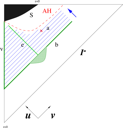
Figure 1: Evolution along outgoing nulls in a portion of a collapse spacetime. Shown are the singularity S, the apparent horizon AH and ${{\cal I}^{-}}\,\,$. Initial conditions are fixed by regularity at the central axis v ($r=0$) and initial data $r$ and $h$ are supplied along the outgoing null b. The arrow indicates the direction of null stepping. Beginning at point a the stepped ingoing nulls are truncated near the apparent horizon. Initial data is then extracted along null e for use in the ingoing null version of the algorithm.

Here we include $r=0$ as the initial point in the grid and identify $u$ as a null coordinate which is constant along outgoing nulls, Fig. 1. We will fix our initial data by specifying $h(u_{0},v)$ and $r(u_{0},v)$ along an initial outgoing null at finite $u=u_{0}$ (‘b’ in Fig. 1). Regularity at $r=0$ (‘v’ in Fig. 1) requires that $h(u,r=0)=\bar{h}(u,r=0)$ (2.8) and $g(u,r=0)=\bar{g}(u,r=0)$ (2.15). Further we will gauge fix $u$ to be proper time at the origin $r=0$, so $g(u,r=0)=\bar{g}(u,r=0)=1$. In light of (2.18), we see that regularity at the origin implies ${\cal{L}}=0$, so the constraint is satisfied everywhere as observed in [18]. We note the explicit quadratures of (2.8), (2.14) and (2.15) subject to these boundary conditions,

$$\bar{h}(u,v) = {1\over r(u,v)}{\int_{0}}^{r(u,v)}h(u,r^{\prime})dr^{\prime}$$ (3.1)

$$g(u,v) = \exp\left[4\pi{\int_{0}}^{r(u,v)}{(h(u,r^{\prime})-\bar{h}(u,r^{\prime}))^{2}\over r^{\prime}}dr^{\prime}\right]$$ (3.2)

$$\bar{g}(u,v) = {1\over r(u,v)}{\int_{0}}^{r(u,v)}g(u,r^{\prime})dr^{\prime}.$$ (3.3)

The choice of $v$ coordinate along the initial null is arbitrary and serves only to identify which grid point belongs to which ingoing null. In practice $v$ is generally taken from a ${{\cal I}^{-}}\,\,$evolution (see section 3.3) so it corresponds to the usual $v\sim t+r$ at past null infinity. The evolution of $r$ and $h$ to the next null is now carried out using (2.16) and (2.19).

As we evolve, the $r$ value of grid locations will decrease eventually becoming negative. The point then becomes unphysical and is dropped from the grid and a new $r=0$ point is interpolated. This is a consistent procedure since the quadratures (3.3) will maintain the correct regularity boundary conditions at the new origin. It is also reassuring to consider the limiting case of the evolution of extremely weak news data, the flat space wave equation. In this limit $u=t-r$, $v=t+r$ and $g=\bar{g}=1$ so $D_{u}(h)=0$. Thus $h(u,v)\propto{\cal{N}}(v)=f^{\prime}(v)$. Substituting this into (3.1) and correcting for normalizations gives

$$\Phi(u,v)={2\over r}{\int_{0}}^{r}{\cal{N}}(v(u,r))dr={1\over{r}}{\int_{u}}^{v}f^{\prime}(v^{\prime})dv^{\prime}={{f(v)-f(u)}\over{r}},$$ (3.4)

so we correctly reproduce the weak field evolution (2.9). In terms of our stepping algorithm this corresponds to our procedure of simply discarding points as they pass to negative values of $r$.

We also monitor the value of

$$\mu={2m\over r}=1-{\bar{g}\over g}$$ (3.5)

along the grid. If $\mu$ approaches 1 (the point ‘a’ in Fig. 1), then we are approaching the apparent horizon. This version of the algorithm cannot proceed past this point since $r$ begins to decrease along an outgoing null as it crosses the apparent horizon, so the $(u,r)$ coordinate system is not even one-to-one. The value of $r$ at the grid point where this limit was exceeded is noted as an estimate of the final black hole size $r_{BH}$, as is an estimate of the asymptotic Bondi mass, the value of $m$ in the outermost grid point.

We now proceed with the evolution by simply discarding the outer parts of the grid where a limit on $\mu$ is exceeded (notice $\mu=0$ at the regular $r=0$ origin as can be seen from a power series expansion of the functions in $r$). This allows us to approach close to the appearance of the singularity at $r=0$. The integration is halted when the outermost value of $r$ is less than some $r_{min}$ and we extract initial data ($u$, $r$ and $\bar{h}$) along the ingoing null containing that point (‘e’ in Fig. 1) for use as initial conditions for the ingoing null phase of the evolution (see section 3.2).

3.2 $v$-mode Stepping on Ingoing Nulls Excluding $r=0$

In this mode we abandon our dependence on regularity at $r=0$. Indeed, generally $r=0$ will be a singular point. The basic algorithm is identical with that described in section 2 but we now reinterpret the ‘$u$’ coordinate to be a conventional $v$ coordinate constant along ingoing nulls. Our region of integration is now bounded by an ingoing null and an outgoing null, Fig. 2. We use the extracted data from the previous $u$-mode integration to provide initial data on the ingoing null (‘e’ in Fig. 2), $u$, $r$ and $h$ (which is obtained from the extracted $\bar{h}$ by numerical differentiation). On the outgoing null boundary (‘b’ in Fig. 2) we similarly extract values for $r$, $\bar{h}$, $g$ and $\bar{g}$, but change $g\rightarrow-g$ and $\bar{g}\rightarrow-\bar{g}$ corresponding to the gauge change $v\rightarrow-v$. This gives us a $v$ coordinate increasing along the outgoing null as implicitly defined by the analog of (2.19),

$$D_{v}(r)={-\bar{g}\over 2}.$$ (3.1)

Equations (2.8), (2.14) and (2.15) are solved using the initial data on the outgoing null, instead of using the regularity conditions at $r=0$.

We now evolve just as before, but in the $v$ direction, stepping the data on the ingoing initial null outwards, employing the same equations as in section 2 with $v$ substituted for $u$. These ensure the solution of all of Einstein’s equations except for the constraint (2.17). But as we have argued through (2.18), we only need to show the constraint is satisfied at one point along each ingoing null. We choose this point to be its intersection with the outgoing null boundary. So we wish to show

$${(g-\bar{g})\over 2r}+{D_{v}(\bar{g})\over\bar{g}}-{D_{v}(g)\over g}-{8\pi r(D_{v}\bar{h})^{2}\over\bar{g}}=0$$ (3.2)

along the outgoing null, where

$$D_{v}(f)=\left(\frac{\partial f}{\partial v}\right)_{u}.$$ (3.3)

By virtue of our definition of $v$ coordinate (3.1) we can replace the $D_{v}$ operator in (3.2) by

$$D_{v}(f)={-\bar{g}\over 2}D_{r}(f)$$ (3.4)

where

$$D_{r}(f)=\left(\frac{\partial f}{\partial r}\right)_{u}.$$ (3.5)

So $D_{r}(f)$ is the same as $f_{,r}$ in the $(u,r)$ coordinate system. Now from (2.8), (2.14) and (2.15) respectively (which were used to construct our original outgoing null data), we have,

$$D_{r}(\bar{h}) = {\hat{h}-\bar{h}\over r}$$ (3.6)

$${D_{r}(g)\over g} = 4\pi{(\hat{h}-\bar{h})^{2}\over r}$$ (3.7)

$$D_{r}(\bar{g}) = {g-\bar{g}\over r}.$$ (3.8)

We have written $\hat{h}$ instead of $h$ to emphasize that it refers to the function $h$ in the old coordinates $(u,r)$. $h$ and $\hat{h}$ are related to the invariant $\bar{h}=\phi$ by $r$ derivatives along different null directions. Substitution of these results into (3.2) yields an identity. So we conclude we have consistent data for an integration of the eoms.

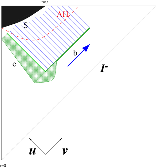
Figure 2: Evolution along ingoing nulls in a collapse spacetime as in Fig. 1. Initial data from the $u$-mode evolution is supplied along the ingoing null e and the outgoing null b. The arrow indicates the direction of null evolution. The ingoing nulls are truncated as they approach the $r=0$ singularity S.

According to a theorem of Christodoulou [20], the apparent horizon will extend outwards from the regular $r=0$ axis in an ‘achronal’ manner, spacelike except for possible null parts. So provided we have penetrated deep enough in $r$ with our ingoing initial null the evolving integration region should encounter the apparent horizon and pass inside. Notice that, unlike in the $u$-mode scheme, $\bar{g}$ can pass through zero and change sign. $\bar{g}=0$ signals the apparent horizon and there is no divergence in the metric functions in the $v$-mode gauge. Once an outgoing null crosses the horizon its $r$ value begins to decrease as it falls in towards the singularity and we truncate the grid again at some fixed $r_{min}$.

Once the horizon appears we have grid points inside falling towards the singularity and those outside flying away, so the region around the horizon quickly empties. We replenish them using a ‘point-splitting’ scheme [28], simply interpolating new points to keep the grid populated. Also the $u$ coordinate grid becomes extremely flat. To integrate to large values of $v$ we would need a ‘gauge-correction’ and to increase efficiency a ‘point-removal’ scheme to eliminate unnecessary points. The extent of the region of spacetime we are interested in has not required these steps.

3.3 ${{\cal I}^{-}}\,\,$-mode Outgoing Null Evolution Excluding $r=0$

Finally, we introduce one more operating mode to bring past null infinity, ${{\cal I}^{-}}\,\,$, into the grid, Fig. 3. We will rescale the auxiliary functions involved in the $u$-mode integration in such a way that derivatives and functions are well defined and finite at ${{\cal I}^{-}}\,\,$. To this end we introduce a compactified $u$ coordinate and $v$ related quantity,

$${\tilde{u}} = {-1\over u}$$ (3.1)

$${\tilde{v}} = u+2r=2r-{1\over{\tilde{u}}}.$$ (3.2)

$v$ will be gauge fixed to equal to ${\tilde{v}}$ at ${{\cal I}^{-}}\,\,$(${\tilde{u}}=0$). This is, as usual, an arbitrary choice since it plays no essential role other than being a label, but (3.2) ensures that $v$ approaches the usual sort of $v\sim t+r$ coordinate at ${{\cal I}^{-}}\,\,$. We also restrict ourself to initial data such that ${\cal{N}}(v)=0$ for $v<v_{0}$. This allows us to impose vacuum boundary conditions along the ingoing boundary null $v=v_{0}$ (‘v’ in Fig. 3) so we are not obliged to include the origin on the grid. To be clear we work in the $({\tilde{u}},v)$ null coordinates, though again we occasionally abuse the notation and regard functions as depending on $({\tilde{u}},{\tilde{v}})$. ${\tilde{v}}({\tilde{u}},v)$ will play a role similar to $r$ in $u$-mode, it will be evolved. Initial data specified at ${{\cal I}^{-}}\,\,$are ${\tilde{v}}(0,v)$ and ${\tilde{h}}(0,v)$. We now define the auxiliary functions, which are rescaled versions of (3.3) modified to contain an inner cutoff radius,

$${\tilde{h}}({\tilde{u}},v) = h(u,v)$$ (3.3)

$${\tilde{\bar{h}}}({\tilde{u}},v) = u\bar{h}={-1\over(1+{\tilde{u}}{\tilde{v}})}\int_{{\tilde{v}}({\tilde{u}},v_{0})}^{{\tilde{v}}({\tilde{u}},v)}{\tilde{h}}({\tilde{u}},{\tilde{v}}^{\prime})d{\tilde{v}}^{\prime}$$ (3.4)

$${\tilde{g}}({\tilde{u}},v) = u(g-1)={-1\over{\tilde{u}}}\left[\exp{(4\pi{\tilde{u}}\int_{{\tilde{v}}({\tilde{u}},v_{0})}^{{\tilde{v}}({\tilde{u}},v)}{({\tilde{h}}({\tilde{u}},{\tilde{v}}^{\prime})+{\tilde{u}}{\tilde{\bar{h}}}({\tilde{u}},{\tilde{v}}^{\prime}))^{2}\over(1+{\tilde{v}}^{\prime}{\tilde{u}})}d{\tilde{v}}^{\prime})}-1\right]$$ (3.5)

$${\tilde{\bar{g}}}({\tilde{u}},v) = u^{2}(\bar{g}-1)={-1\over(1+{\tilde{u}}{\tilde{v}})}\int_{{\tilde{v}}({\tilde{u}},v_{0})}^{{\tilde{v}}({\tilde{u}},v)}{\tilde{g}}({\tilde{u}},{\tilde{v}}^{\prime})d{\tilde{v}}^{\prime}.$$ (3.6)

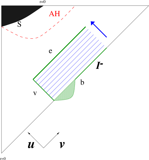
Figure 3: Evolution along outgoing nulls from ${{\cal I}^{-}}\,\,$in a collapse spacetime as in Fig. 1. Initial data is given along a portion of ${{\cal I}^{-}}\,\,$, b, and vacuum initial data is set along the ingoing null v. The arrow indicates the direction of null stepping. Data at finite $r$ is extracted along a final outgoing null e.

In terms of these variables the evolution equations read

$$D_{\tilde{u}} = u^{2}D_{u}$$ (3.7)

$$D_{\tilde{u}}{\tilde{v}} = -{\tilde{\bar{g}}}$$ (3.8)

$$D_{\tilde{u}}{\tilde{h}} = {{-({\tilde{g}}+{\tilde{u}}{\tilde{\bar{g}}})({\tilde{h}}+{\tilde{u}}{\tilde{\bar{h}}})}\over(1+{\tilde{u}}{\tilde{v}})}.$$ (3.9)

${{\cal I}^{-}}\,\,$(${\tilde{u}}=0$) is now a regular null on the grid. Explicitly, at ${{\cal I}^{-}}\,\,$(3.5) can be replaced by the only non-vanishing term in its power series expansion in ${\tilde{u}}$,

$${\tilde{g}}(0,v) =-4\pi\int_{{\tilde{v}_{0}}(0,v_{0})}^{{\tilde{v}}(0,v)}{\tilde{h}}(0,{\tilde{v}}^{\prime})^{2}d{\tilde{v}}^{\prime}.$$ (3.10)

The evolution is halted when the innermost point of the data reaches a specified finite $r$ and data is extracted. It can then be connected through vacuum to the origin and evolution is continued in $u$-mode.

4 Numerics, Tests and Verifications

We use the lowest order algorithms still compatible with quadratic convergence. The $r$ integrations along the nulls are carried out using the trapezoid rule, the null stepping is carried using a second order Runge-Kutta method and linear interpolation is used where necessary. Besides the advantage of simplicity, these methods work tolerably well even with data of low differentiability (e.g. [12] (4.37)).

It is useful to choose an analytic test case exhibiting features in common with scalar collapse. A simple case is spatially flat FRW scalar collapse, the simplest version of the PBB. While too simple to provide a good test of an $(r,t)$ code, having no spatial gradients, when written in radial null coordinates we will see it has features in common with radial scalar collapse and has non-zero gradients in the null directions.

We write the FRW metric

$$ds^{2}=-dt^{2}+a(t)^{2}(dR^{2}+R^{2}d\omega^{2})$$ (4.1)

in terms of conformal time $\eta$,

$$ds^{2} = a(\eta)^{2}(-d\eta^{2}+dR^{2}+R^{2}d\omega^{2})$$ (4.2)

$$\eta = \int^{t}{1\over a(t^{\prime})}dt^{\prime}.$$ (4.3)

Introducing null coordinates defined by conformal time at the origin, $\hat{u}=\eta-R$ and $v=\eta+R$, we can write the PBB solution,

$$a(\eta) = \sqrt{\eta\over\eta_{0}},\,\,\eta<0$$ (4.4)

$$\phi(\eta) = {-\sqrt{3}\over{2\sqrt{\pi}}}\log(a(\eta)),$$ (4.5)

in terms of these null coordinates. Finally we replace the $\hat{u}$ coordinate with the $u$ coordinate defined in terms of proper time at the origin

$$\hat{u}=\eta_{0}\left[{u\over u_{0}}\right]^{2\over 3},$$ (4.6)

where $\eta_{0}=3u_{0}/2$ is a chosen initial time ($a(\eta_{0})=1$). Finally we change to the area $r$ coordinate by $R={r/a(u,v)}$.

The resulting solution has divergent news at ${{\cal I}^{-}}\,\,$, requiring us to specify initial data at finite $u$, but the rest of the algorithm proceeds just as with a realistic collapse since this solution has a spacelike singularity at $v=-\hat{u}$ ($\eta=0$) hidden by a spacelike apparent horizon at $v=-\hat{u}/3$, allowing us to test the horizon crossing and $v$-mode approach to the $r=0$ singularity.

First we verify the order of convergence of the algorithm by checking it against the exact solution (4.5). We take initial $r$ and $h$ data from the exact solution at $u_{0}=-2$, $-2<v<0.5$. The data is then evolved to $u=-1$ and the results are compared with the exact solution. Fig. 4 shows the logarithm (base 10) of the absolute value of the largest error, $\Delta$, in $\phi$ on the grid versus the logarithm of the number of initial grid points $n=50,100,200,400,800$. It is clearly almost exactly quadratically convergent.

The full algorithm is then deployed to test the near $r=0$ approach to the singularity. Anticipating the asymptotic analysis of section 6, we numerically extract the small $r$ behavior of the dilaton near the singularity. As we will discuss this is expected to be of the form $\Phi(v)=2\alpha(v)\log(r)$, and since this is homogeneous and isotropic collapse, the value of $\alpha(v)=-\sqrt{3}$ is expected. Using 400 points on the grid, the horizon first appears at $r=0.42$ (marked by $\mu>0.98$) and the $v$-mode integration is pushed to $r=0.001$. The results are shown in the second figure in Fig. 4. We show the values of $\alpha^{2}(v)$ extracted from the asymptotics of $\Phi$, $m$ and $g$. The small $v$ deviation from the asymptotic values are expected, since the null geodesics have not yet penetrated close to the singularity, see Fig. (2). In this particular run we find $\alpha(v)\rightarrow-1.728$ compared with $-\sqrt{3}=-1.732$, confirming we can reach near enough to the singularity to extract asymptotic values of $\alpha(v)$. As we will discuss further in section 6, this is the quantity which will characterize the cosmological nature of the collapse.

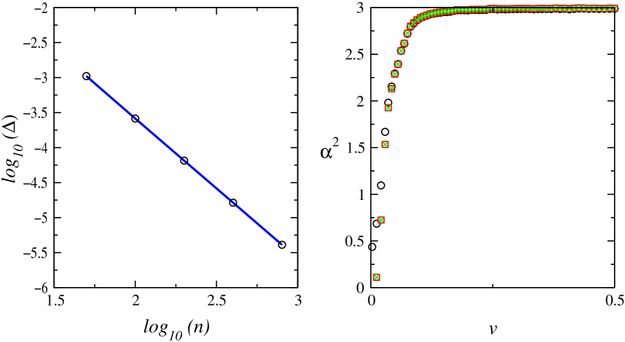
Figure 4: Left: the log of the maximum difference, $(\Delta)$, of the numerical integration of $\phi$ from the exact PBB solution (4.5) plotted versus the log of the number of grid points $n$ for $n=50,100,200,400,800$. Right: a numerical extraction of the asymptotic value of $\alpha^{2}(v)$ for the same solution from $\phi$ ($\circ$), $m$ ($\Box$) and $g$ ($\times$) over a range of $v$.

Among other tests of the code, we repeat a calculation of the collapse of a initial pulse in $\phi$ and compare with the data presented in [30] with good agreement. We note that although his integration proceeds several orders of magnitude deeper into the black hole than we do, he finds almost no change in the asymptotic $\alpha(v)$ over the last few orders of magnitude, giving us some confidence we can get a good idea of the asymptotic behavior with a relatively shallow penetration inside the apparent horizon. We also compare with other numerical results (e.g. [26]) and other exact solutions. In addition we verify agreement between the various stepping modes on regions of overlap and numerically evaluate the constraint. All tests indicate the code produces stable integrations in agreement with others in the literature.

5 Collapse Criteria

In attacking the question of the structure of scalar collapse, the authors of [12] develop a perturbative expansion of the weak-field behavior in terms of powers of the strength of the news function, as defined by (2.10). They obtain a concise result for the quadratic approximation of the mass ratio $\mu=2m/r$ for news data ${\cal{N}}(v)=f^{\prime}(v)$,

$$\mu_{2}(u,v)=\frac{1}{v-u}\int_{u}^{v}dx\,f^{\prime 2}(x)-\left[\frac{f(v)-f(u)}{v-u}\right]^{2}\,.$$ (5.1)

They further simplify by noting that if one defines the average of a function by

$$\langle g\rangle(u,v)={1\over v-u}\int_{u}^{v}g(x)dx,$$ (5.2)

and defines a variance by

$$Var(g)(u,v)=\langle(g-\langle g\rangle(u,v))^{2}\rangle(u,v),$$ (5.3)

this becomes just

$$\mu_{2}(u,v)=Var({\cal{N}})(u,v).$$ (5.4)

Since $\mu=1$ is the signal of the formation of an apparent horizon leading to inevitable collapse, this leads them to define the maximum of its quadratic approximation

$$BDV({\cal{N}})=\sup_{u,v\atop u\leq v}Var({\cal{N}})(u,v),$$ (5.5)

and state that news data will collapse if it satisfies an inequality of the form

$$BDV({\cal{N}})\geq C({\cal{N}}),$$ (5.6)

where $C({\cal{N}})$ depends only on the shape of the news and not on its amplitude. So $C({\cal{N}})$ measures one aspect of the departure from linearity of the evolution of ${\cal{N}}$. The usefulness of a criterion of this form is measured by the complexity of the functional $C({\cal{N}})$ and would be maximized if it could be replaced by a constant. But it could still be of some use if $C({\cal{N}})$ would be bounded for a family of ‘reasonably generic’ initial data and perhaps only depend weakly on ${\cal{N}}$. Aside from its simplicity the criterion is suggestive because it shares the exact scale invariance of the massless gravity-scalar system ($r\rightarrow kr$). The perturbative expansion leads them to estimate $C({\cal{N}})=O(1)$. They also examine an exact collapse, [34], and find $C({\cal{N}})=1/4$ for this particular case.

To examine this numerically, we select a family of news data depending on a number of parameters, map the boundary between collapse and dispersal in this parameter space and then evaluate $BDV({\cal{N}})$ along this boundary. Specifically we define a ‘wavelet’,

$$n(v)=a\cos({{2\pi(v-v_{0})f}\over w})\exp(-{(v-v_{0})^{2}\over w^{2}}).$$ (5.7)

Assigning ${\cal{N}}(v)=n(v)$ we see that this initial data has four parameters, amplitude $a$, frequency $f$, width $w$ and center $v_{0}$. $v_{0}$ is clearly irrelevant since translation of news data just shifts the value of $u$ where the pulse approaches the origin. The irrelevance of $w$ is less obvious, but comes from the scale invariance of the system. So shifting $w$ can change the size of black hole formed, but cannot affect whether it will form. We have verified the numerics show this same insensitivity. So we will set these variables arbitrarily ($v_{0}=-2$, $w=1$). We then choose a value for $f$ and locate a value of $a$ where the data disperses and a larger value of $a$ where it collapses. Searching by bisection we find the critical collapse amplitude $a_{0}(f)$ for this value of $f$. Doing this for a number of values of $f$ allows us to collect a set of critical values of $a_{0}(f)$ for different values of $f$. Finally calculating $BDV({\cal{N}})$ for these critical collapse news functions gives us a cross-section of the shape of $C({\cal{N}})$ across this family of functions.

Before doing this we check that the algorithm can accurately approach the collapse threshold by extracting the Choptuik exponent of the scaling of the black hole radius with the difference in amplitude from the critical amplitude

$$r_{BH}\propto(a-a_{0})^{\gamma},$$ (5.8)

where the constant $\gamma$ is expected to depend only on the type of collapsing matter and not on the details of the waveform [24]. The results for $f=0$ news data are shown are shown in the first graph in Fig. 5. A best fit line to the first five points yields a slope of $\gamma=0.373$. This can be compared with other values in the literature, 0.376 in the first reference in [24] or 0.374 in [29].

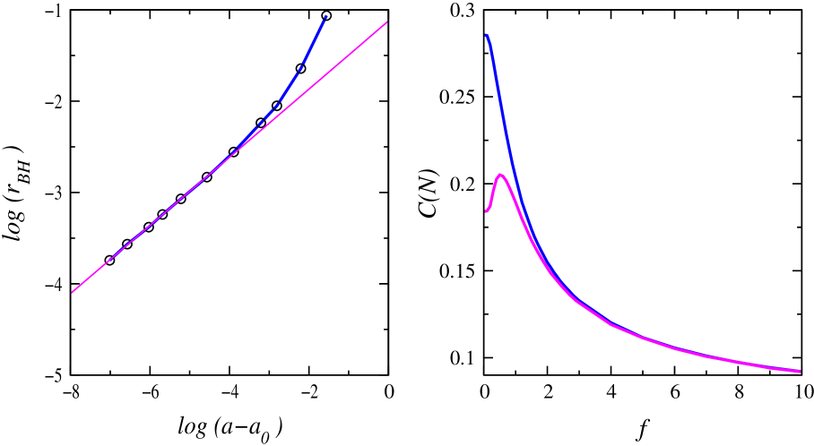
Figure 5: Left: Choptuik scaling for $f=0$, $w=1$ news (${\cal{N}}(v)=n^{\prime}(v)$ (5.7)). Log of the black hole radius versus log of the difference between the amplitude $a$ and the critical amplitude $a_{0}=0.1896$. A best fit line to the first five points is also shown with slope 0.373. Right: The $C({\cal{N}})$ functional appearing in the $BDV$ criterion as a function of frequency $f$. On the upper trace ${\cal{N}}(v)\propto n(v)$ and on the lower ${\cal{N}}(v)\propto n^{\prime}(v)$.

We will use the wavelet data $n(v)$ as initial data ${\cal{N}}(v)$. We also take a second family of news functions ${\cal{N}}(v)\propto n^{\prime}(v)$ While looking substantially different for low frequencies where the derivative of $n(v)$ is dominated by the gaussian component, at higher frequencies these functions will differ mainly by a phase coming from the oscillatory component. The dependence of $C({\cal{N}})$ as a function of $f$ for these two families is shown in the second graph in Fig. 5.

As one might expect, the phase difference at higher frequencies makes little difference in collapse, as the numerics confirm by the convergence of the two curves. The most remarkable feature of the curves is their decline at high frequencies. If $C({\cal{N}})$ has no lower bound, then in light of the scale invariance of the collapse this suggests that a very long wave train of very low amplitude news may in fact be gravitationally unstable to collapse. Unsystematic experiments have produced data which collapse at $BDV({\cal{N}})$ as low as 0.06, but numerical experiments alone cannot give a definitive answer. This complements analysis in [12] suggesting that for extremely slowly decaying news data $C({\cal{N}})$ may go to zero.

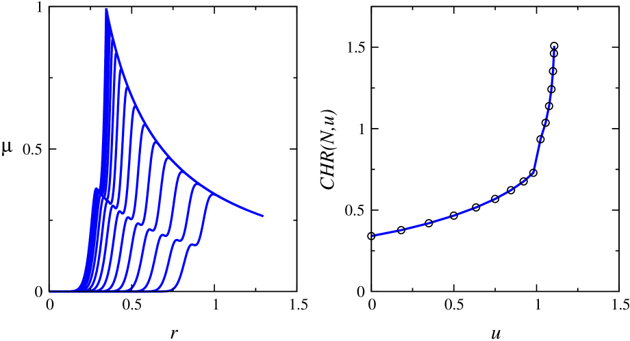
Figure 6: Collapse with ${\cal{N}}\propto n^{\prime}(v)$, $f=0$, $w=1$ with amplitude normalized to 0.4. Left: the evolution of $\mu$ at several successive values of $u$ approaching horizon formation. Right: The values of $CHR({\cal{N}},u)$ for these values of $u$.

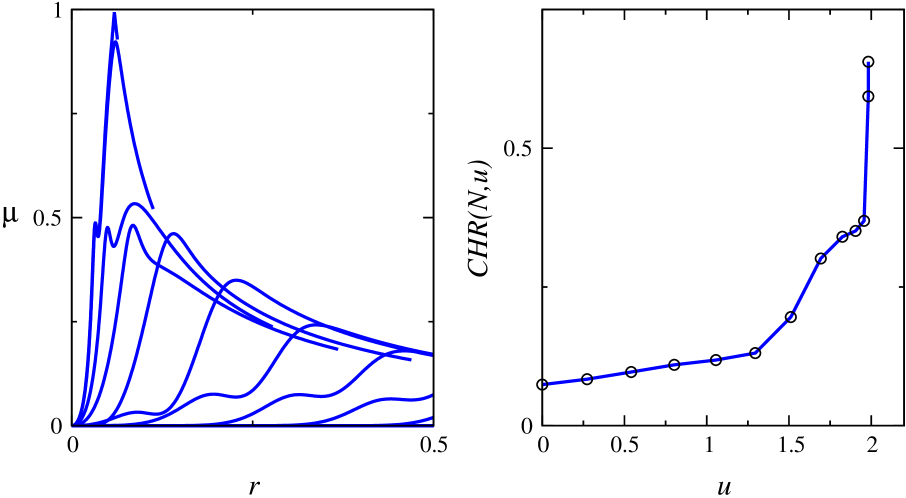
Figure 7: Collapse with ${\cal{N}}\propto n^{\prime}(v)$, $f=0$, $w=1$ and amplitude normalized to 0.2. Left: the evolution of $\mu$ at several successive values of $u$ approaching horizon formation. Right: The values of $CHR({\cal{N}},u)$ for these values of $u$.

We also wish to make some comparison of this criteria with a rigorous sufficient criterion of Christodoulou [20]. It states that if for some value of $u$

$$\frac{2\Delta m}{\Delta r}\geq\left[\frac{r_{1}}{r_{2}}\,\log\left(\frac{r_{1}}{2\Delta r}\right)+\frac{6r_{1}}{r_{2}}-1\right]\,,$$ (5.9)

where $r_{1}<r_{2},r_{2}\leq 3r_{1}/2,\Delta r=r_{2}-r_{1}$ and $\Delta m=m(u,r_{2})-m(u,r_{1})$, then future collapse is inevitable. In physical terms it states that if the energy flux contained between two spheres is larger than a function involving the ratio of the two radii, then we can predict collapse.

Defining $C_{l}({\cal{N}},u,r_{1},r_{2})$ to be the left hand side of this inequality and $C_{r}({\cal{N}},u,r_{1},r_{2})$ to be the right and

$$CHR({\cal{N}},u)=\sup_{r_{1},r_{2}\atop r_{1}<r_{2}\leq 3r_{1}/2}C_{l}({\cal{N}},u,r_{1},r_{2})/C_{r}({\cal{N}},u,r_{1},r_{2}),$$ (5.10)

we can then state the criterion as simply that $CHR({\cal{N}},u)\geq 1$ is sufficient to insure collapse.

As this criterion needs to be applied at finite $u$ (since $m\rightarrow 0$ as $u\rightarrow-\infty$, $CHR$ can never predict collapse at large negative $u$) and the $BDV$ criterion needs to be applied at ${{\cal I}^{-}}\,\,$, a direct comparison is impossible. The best we can do to investigate its strength in predicting collapse is to ask how early it can predict collapse before the formation of the apparent horizon.

To test this we form initial data ${\cal{N}}\propto n^{\prime}(v)$ for $f=0$, $w=1$ corresponding to a gaussian pulse in $\phi$. Since the normalized amplitude for threshold collapse of this data set is found to be 0.1896, we first normalize the amplitude of ${\cal{N}}(v)$ to 0.40 (Fig. 6) to investigate a heavy collapse and then to 0.20 (Fig. 7) to investigate a near critical collapse. In the first graph in each figure we show the profile of $\mu$ versus $r$ for a number of values of $u$ leading up to horizon formation. In the second graph we show the corresponding values of $CHR({\cal{N}},u)$. In the first case we find that even for the heavier collapse the criterion predicts the appearance of the apparent horizon only rather near to its formation. In the second we do not get near enough to the horizon formation for the criterion to ever predict the collapse. This would seem to point to the strong nonlinearities involved in the horizon formation, particularly in the near critical region where a very small change in the news amplitude leads to a very large change in the largest value of $\mu$ eventually attained.

6 Black Hole Interior Asymptotics and the PBB

The proposal that ‘the PBB is as generic as gravitational collapse’ is the central proposal of [12], and the measure of validity of this proposal lies in the interior of the black holes produced by massless scalar collapse. Since inside the black holes the $r$ coordinate becomes timelike, the geometry there describes a spacelike hypersurface approaching a future singularity and the geometry is naturally interpreted as cosmological. And since the dilaton, the scalar field, also generically shows runaway behavior, this suggests that the black hole interior when interpreted in the string frame may generically exhibit the pole-law inflation of the PBB scenario. With a graceful exit mechanism (possibly due to corrections to the lowest order perturbative action coming from large curvature and strong coupling) to regulate the approach to the singularity, the black hole interior may be regarded as a ‘baby universe’. The first step is to check that the regime where the dynamics is dominated only by the lowest order action without corrections has some resemblance to the PBB scenario.

Thanks to the work of [14] it is known that the interior solutions for generic initial data (without additional field content) will be asymptotically velocity dominated, a ‘quiescent cosmological singularity’. The final cosmological approach to the singularity will take the form of Kasner evolution, an FRW evolution modified by some degree of anisotropy. As the PBB form of inflation is known not to wash out anisotropy [32] (as is clear in our case, since once we are into the Kasner regime the degree of anisotropy freezes and remains constant), unless we take the opinion that the graceful exit will also cure this problem, we should look for features of generic gravitational collapse that will also select for isotropy. Working in spherical symmetry takes us part of the way to isotropy. since this forces two of the Kasner exponents to be equal, but this restriction is quite artificial. Nonetheless, if we can show collapse favors a third exponent equalling the other two, this would be some evidence a non-spherical collapse could also favor isotropy.

In addition to relative isotropy, a ‘good’ PBB collapse should satisfy several requirements related to APT. The dilaton should be increasing with $\Phi<<0$ and the spacetime curvature should be small at the entrance to the asymptotic regime to ensure the lowest order action is valid for a sufficiently large number of e-folds of dilaton driven inflation. But we observe that any solution can be mapped to a solution of arbitrarily small curvature and weak coupling by applying a constant shift of the dilaton $\Phi\rightarrow\Phi+C$ or performing a scale transformation $\Phi(r)\rightarrow\Phi(kr)$ (changing the scalar curvature $R\rightarrow R/k^{2}$) without affecting the asymptotic Kasner behavior, as will be seen from the following analysis.

In this scenario the need for a ‘tuning’ of these two classical moduli of the collapse is acknowledged. But due to the invariances of the system we should also expect collapses to occur on all size scales and couplings. Only sufficiently large and weakly coupled collapses will lead to universes such as we occupy. Others are regarded as stillborn [35]. This also makes the question of the degree of fine-tuning subject to anthropic considerations, since the birth of a universe is no longer a unique event. With these invariances, the task left to a numeric code will be to analyze the relative degree of isotropy in the cosmology within the collapse as a function of the shape and amplitude of the initial news data.

We first recall the small $r$ asymptotics derived in [12, 30] (and confirmed numerically in [30]) and rederive the relation between the asymptotics of the different functions. We start with the dominant terms in the growth of the scalar as we approach the $r=0$ singularity,

$$\Phi(v,r)\sim 4\sqrt{\pi}\bar{h}\sim 2\alpha(v)\log r+C_{\phi}(v).$$ (6.1)

Using the defining relation for $h$ (2.8) we easily have,

$$h(v,r)=\bar{h}(v,r)+{\alpha(v)\over{2\sqrt{\pi}}}.$$ (6.2)

Inserting this into (2.14) we find that to leading order,

$$g(v,r) \sim C_{g}(v)r^{\alpha^{2}(v)}$$ (6.3)

$$\bar{g}(v,r) \sim {{C_{\bar{g}}(v)}\over r}.$$ (6.4)

Recalling the relation $\bar{g}/g=1-2m/r$, we have in the limit of small $r$,

$$m(v,r)\sim C_{m}(v)r^{-\alpha^{2}(v)}.$$ (6.5)

So we see that nature of the evolution near the singularity is controlled entirely by $\alpha(v)$. We will next see how this $\alpha(v)$ is related to the Kasner exponents in the string and Einstein frame. We will follow the discussion of [12], filling in some details and omitting some more general discussions.

Inserting the limiting behavior above into (2.4) we find

$$ds^{2}\sim r^{\alpha^{2}(v)-1}~{}dv^{2}+r^{\alpha^{2}(v)}~{}dv~{}dr+r^{2}d\omega^{2}.$$ (6.6)

Here we have omitted all $C(v)$ factors (in the asymptotic Kasner region they are locally nearly constant) and numerical constants since they can finally be absorbed into rescalings of the coordinates. By completing the square, this can be written as

$$ds^{2}\sim-{1\over 4}r^{\alpha^{2}(v)+1}dr^{2}+(dv+{r\over 2}dr)^{2}r^{\alpha^{2}(v)-1}+r^{2}d\omega^{2}.$$ (6.7)

Changing to Einstein frame cosmic time via

$$(-t_{E})\sim r^{{\alpha^{2}(v)+3}\over 2},$$ (6.8)

this becomes (again omitting constants)

$$d{s_{E}}^{2} \sim -d{t_{E}}^{2}+(-t_{E})^{2\lambda_{1}}d{x_{1}}^{2}+(-t_{E})^{2\lambda_{2}}(d{x_{2}}^{2}+d{x_{3}}^{2})$$ (6.9)

$$\Phi \sim \gamma(v)\log(-t_{E}),$$ (6.10)

where $x_{2}$ and $x_{3}$ are the spacelike coordinates of spherical symmetry (in $d\omega^{2}$) and $x_{1}$ is the remaining spacelike direction and

$$\lambda_{1}(v)=\frac{\alpha^{2}(v)-1}{\alpha^{2}(v)+3}\,,\quad\quad\lambda_{2}(v)=\frac{2}{\alpha^{2}(v)+3}\,,\quad\quad\gamma(v)=\frac{4\alpha(v)}{\alpha^{2}(v)+3}\,.$$ (6.11)

We complete the transition into the string frame by applying (2.2) and changing to string frame cosmic time by

$$-t_{S}=(-t_{E})^{{2+\gamma(v)}\over 2}$$ (6.12)

obtaining

$$d{s_{S}}^{2} \sim -d{t_{S}}^{2}+(-t_{S})^{2\alpha_{1}}d{x_{1}}^{2}+(-t_{S})^{2\alpha_{2}}(d{x_{2}}^{2}+d{x_{3}}^{2})$$ (6.13)

$$\Phi \sim \sigma(v)\log(-t_{S}),$$ (6.14)

where

$$\alpha_{1}(v) = \frac{\alpha^{2}(v)+2\alpha(v)-1}{\alpha^{2}(v)+2\alpha(v)+3},\quad\alpha_{2}(v)=\frac{2(\alpha(v)+1)}{\alpha^{2}(v)+2\alpha(v)+3},$$

$$\sigma(v) = \frac{4\alpha(v)}{\alpha^{2}(v)+2\alpha(v)+3}.$$ (6.15)

We can now state the requirement for a ‘good’ PBB collapse in terms of $\alpha(v)$. Consistent with inflationary behavior, we should at least require all directions are expanding (all string Kasner exponents negative) and an increasing dilaton. These requirements can be met by looking for regions where $-1-\sqrt{2}<\alpha(v)<-1$ with $\alpha(v)=-\sqrt{3}$ corresponding to exact isotropy. Since changing the sign of ${\cal{N}}(v)$ reverses the sign of $\alpha(v)$, we will be concerned with the magnitude of $\alpha(v)$.

While it is clearly difficult to generalize about the infinite dimensional space of all possible initial data, we will present several data sets extracted from the many we have run looking for general trends. We choose a collapsing data set and extract values of $\alpha^{2}(v)$ by fits to the small $r$ data from (6.1), (6.3) and (6.5). We will take agreement between these values to indicate that we are qualitatively in the asymptotic regime.

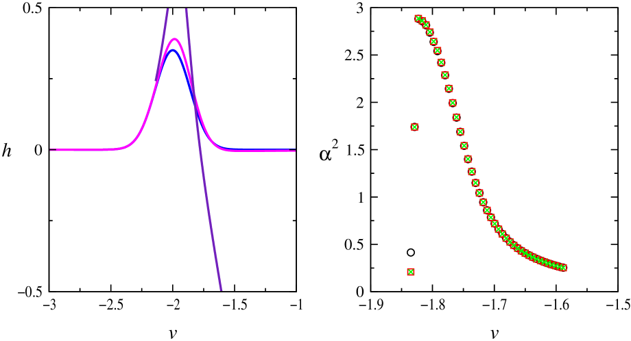
Figure 8: Collapse of an amplitude 0.35 gaussian news pulse, left: $h$ as a function of $v$ at ${{\cal I}^{-}}\,\,$, the end of ${{\cal I}^{-}}\,\,$evolution and near horizon formation (in order of increasing amplitude). Right: the extracted values of $\alpha^{2}(v)$ from $\phi$ ($\circ$), $m$ ($\Box$) and $g$ ($\times$).

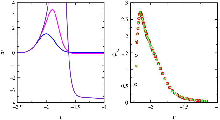
Figure 9: Collapse of an amplitude 1.5 gaussian news pulse, left: $h$ as a function of $v$ at ${{\cal I}^{-}}\,\,$, the end of ${{\cal I}^{-}}\,\,$evolution and near horizon formation (in order of increasing amplitude). Right: the extracted values of $\alpha^{2}(v)$ from $\phi$ ($\circ$), $m$ ($\Box$) and $g$ ($\times$).

In the first set, Fig. 8, we choose gaussian news, $a=0.35$, $f=0$, $v_{0}=-2$ and $w=0.2$ (5.7). This is somewhat over the critical amplitude of $a_{0}=0.309$. The first graph shows the profile of $h$ at ${{\cal I}^{-}}\,\,$, at the end of the ${{\cal I}^{-}}\,\,$evolution and at the point where $\mu>0.99$ and it shortly after forms a black hole of radius $r_{BH}=0.1349$. We run the $v$-mode integration over the region near the $r=0$ singularity to extract the $\alpha^{2}(v)$ values from data going as deep as $r_{min}=0.00008$. As the second figure shows, this includes the region of significant deviation of $\alpha(v)$ from zero. At larger values of $v$, $\alpha(v)$ is running to its Schwarzschild value of zero, in accordance with the dictum ‘black holes have no hair inside or out’. We do find a region of $\alpha^{2}(v)>1$, corresponding a minimal inflationary criterion of ‘all-directions expanding’, and further the maximum value of $\alpha^{2}(v)\sim 3$ reached corresponds to relative isotropy, although it is a narrow region very near to the initial $v$ of the black hole formation. The innermost points represent ingoing nulls that fail to penetrate into the asymptotic region, so the apparent fall-off in the value of $\alpha(v)$ should not be taken seriously. We also note that the onset of black hole formation occurs as the end of the pulse is striking the origin.

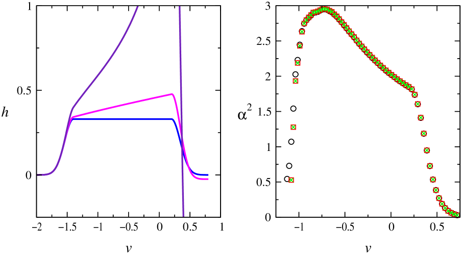
Figure 10: Collapse of a lengthened gaussian pulse, left: $h$ as a function of $v$ at ${{\cal I}^{-}}\,\,$, the end of ${{\cal I}^{-}}\,\,$evolution and near horizon formation (in order of increasing amplitude). Right: the extracted values of $\alpha^{2}(v)$ from $\phi$ ($\circ$), $m$ ($\Box$) and $g$ ($\times$).

In the second set, Fig. 9 we raise the amplitude to $a=1.5$, forming a black hole of radius $r_{BH}=3.495$. We cut off at $r_{min}=0.002$. The qualitative results are quite similar to the first case, pointing again to a small relatively isotropic region corresponding to in a narrow region close to the onset of black hole formation. With the increased amplitude this now occurs when the leading surface of the pulse arrives at the origin.

In the third set, Fig. 10 we extend a gaussian pulse of width 0.2 by adding a flat portion of $v$ length 1.6 in the center of the pulse. We also tune the amplitude to 0.33 so the apparent horizon forms as the flat part of the pulse is striking the origin, although the wave form is no longer flat by then. This time the closeness of the approach to $\alpha^{2}=3$ is striking.

Finally, in the fourth set we send in additional pulses after the first. We also vary the exact form of the initial news data to

$$h(v)=a\sin^{2}({{\pi(v-v_{0})}\over w})$$ (6.16)

with $v_{0}=-2$, $a=0.4$ and $w=1$, and setting $h=0$ outside of four peaks of the news function. Again we find an initial approach to quasi-isotropy and notice that further incoming news data after the formation of the black hole does not have much effect on interior asymptotics.

Comparison of these data with our criteria for a ‘good’ initial PBB leads to limited good news. Large regions of the black hole interior do not reach strong enough gradients in $\Phi$ to meet the ‘all directions expanding’ criterion, much less isotropy. On the other hand there is a strong hint that there may be generically a small region very close the initial point of singularity formation where these requirements are met.

Indeed we note that as we approach smaller and smaller $r$, closer and closer to the first appearance of the apparent horizon at the origin, the asymptotic $\alpha^{2}(v)$ seems to approach 3 and seems to resist exceeding this value. This tempts us to conjecture that singularity onsets in spherical symmetry may approach exact isotropy. This is also suggested by the fact the regular $r=0$ origin is a point of exact isotropy before the collapse, so this quality may extend into the singular region. While suggestive, we have been unable to verify this analytically. However, this would imply the occurrence of this near isotropic region may come from the exact spherical symmetry imposed, so it would not clearly extend to nonspherical collapse.

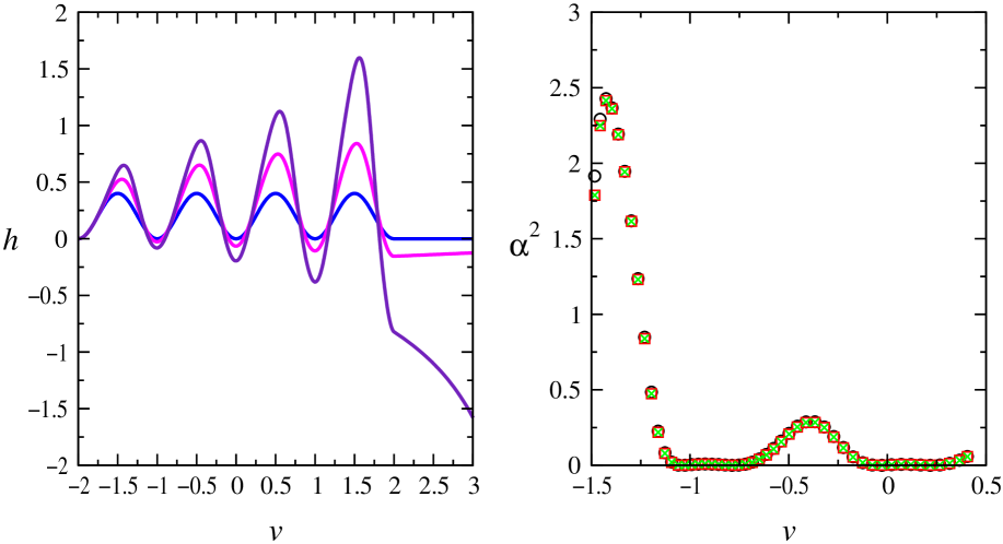
Figure 11: Collapse of a wave train, left: $h$ as a function of $v$ at ${{\cal I}^{-}}\,\,$, the end of ${{\cal I}^{-}}\,\,$evolution and near horizon formation (in order of increasing amplitude). Right: the extracted values of $\alpha^{2}(v)$ from $\phi$ ($\circ$), $m$ ($\Box$) and $g$ ($\times$).

This singularity onset region is also the most numerically difficult to reach and our results so far are hardly conclusive. Analyzing the exact solution ([12] (4.37)) we find it corresponds to $\alpha^{2}(v)=1$. But this solution is neither asymptotically flat nor differentiable at singularity onset, so it may not be representative of more physical collapse data. There also seems to be some trend for near critical collapses to reach higher levels of isotropy, but it is not clear whether this is because the isotropic regions are absent for heavier collapse or that we are simply unable to reach them.

While we conclude the string frame near-isotropy region seems to be generically small (though in a way difficult to quantify exactly), it does seem to be present. Further, as suggested in [36], an initially small isotropic region may grow preferentially relative to its more anisotropic neighbors. Along a slice of constant string frame time (where $t_{S}=0$ is the time of singularity, lacking a graceful exit), the volume of space per unit $dv$ goes as

$$Vol(t_{S},v)=(-t_{S})^{\Sigma\alpha_{i}(v)}.$$ (6.17)

This expansion rate is indeed maximized at $\alpha(v)=-\sqrt{3}$ with $\Sigma\alpha_{i}(v)=-\sqrt{3}$. Since successful PBB inflation is expected to be accompanied by a large growth in $\Phi$, in turn giving many e-folds in string time and in turn of the scale factor, this would seem to say that even an initially small region of isotropy could be exponentially enhanced over its neighbors having less negative exponents of growth rate.

However, this process of comparing growth rates at different places at the same ‘time’ requires singling out a particular foliation of spacelike hypersurfaces. For example, computing the string frame volume growth rates along slices of constant $t_{E}$ or constant $r$ results in a preference for $\alpha(v)$ with relatively strong anisotropy. Given this ambiguity we need to invoke some physical reason for a given choice of foliation. This choice should have something to do with the details of the final graceful exit mechanism but it is not clear to us how to make this more precise without choosing some family of observers to give the proper weight to different regions. Perhaps, finally, these observers should correspond to the locations of future civilizations who could observe this anisotropy. For a Bayesian look at this possibility we refer again to [12], since it is not clear to us that the numerics can add quantitatively to this discussion.

Nevertheless, we routinely find collapses featuring regions of $\alpha(v)<-1$ and indeed approaching isotropy, confirming the general picture of ‘ballooning patches of inflating space’ in [12].

7 Conclusions

We have numerically investigated massless scalar collapse in spherical symmetry in the context of its possible role as a precursor for a PBB inflationary cosmology. We find evidence that such collapses do provide plausible precursors. Our most interesting conclusion based on this preliminary survey, that there seems to be a region of substantial isotropy very near the initial appearance of the singularity on the central axis, will need to be investigated further. It lies in a region that is numerically difficult to reach and it would be much more satisfying to have some analytical understanding of this phenomenon, especially the degree to which it is particular to spherical symmetry. This conclusion also will need to be qualified to the degree to which the additional field content of string theory can spoil this behavior.

We have also investigated a proposed collapse criterion [12]. We find suggestions, again at the fringes of our numerical reach, that special forms of news data, specifically long trains of low amplitude waves, can collapse even though the criterion would suggest they should remain perturbative. In an extreme form this phenomenon would suggest that perhaps a very long train of arbitrarily low amplitude may be capable of collapse through a long slow buildup of non-linearity. While this seems somewhat physically unlikely it would be interesting to try to get some sort of analytical handle on this sort of behavior as well.

8 Acknowledgements

The author wishes to thank Gabriele Veneziano for his continued support of this project and his valuable suggestions and the CERN Theory Division for their hospitality. Also thanks for useful talks and comments from Alessandra Buonanno, Thibault Damour, Vincent Montcrief, Phillipos Papadopoulus, I. M. Segal, Reza Tavakol and Carlo Ungarelli. We also express gratitude for computational facilities provided by the UMS CNRS/Polytechnique MEDICIS and CERN.

References

- [1] J. Polchinski, String Theory (Cambridge University Press, 1998).
- [2] A. Guth, Phys. Rev. Lett. 49 (1982) 1110; A. Linde, Phys. Lett. B129 (1983) 177; A. Linde, Phys. Lett. B175 (1986) 395; K.A. Olive, Phys. Rep. 190 (1990) 307.
- [3] J. Lidsey, D. Wands and E. Copeland, Phys. Rep. 337 343.
- [4] J. Ellis, K. Enqvist, D.V. Nanopoulos and M. Quiros, Nucl. Phys. B277 (1986) 231; K. Maeda and M.D. Pollack, Phys. Lett. B173 (1986) 251, P. Binetruy and M.-K. Gaillard, Phys. Rev. D34 (1986) 3069, R. Brustein and P. Steinhardt, Phys. Lett. B302 (1993) 196.
- [5] G. Veneziano, Phys. Lett. B265 (1991) 287; M. Gasperini and G. Veneziano, Astropart. Phys. 1 (1993) 317; Phys. Rev. D50 (1994) 2519; G. Veneziano, [hep-th/0002094]; For an updated list of references visit the web page http://www.to.infn.it/gasperin/.
- [6] R. Brustein and G. Veneziano, Phys. Lett. B329 (1994) 429; N. Kaloper, R. Madden and K.A. Olive, Nucl. Phys. B452 (1995) 677; M. Gasperini and G. Veneziano, Gen. Rel. Grav. 28 (1996) 1301; R. Easther and K. Maeda, Phys. Rev. D54 (1996)0 7252; M. Gasperini, M. Maggiore and G. Veneziano, Nucl. Phys. B494 (1997) 315; R. Brustein and R. Madden, Phys. Rev. D57 (1998) 712; M. Maggiore, Nucl. Phys. B525 (1998) 413; R. Brandenberger and D. Easson, JHEP 03 (1999) 009; R. Brustein and R. Madden, JHEP 07 (1999) 006; S. Foffa, M. Maggiore and R. Sturani, Nucl. Phys. B552 (1999) 395; A. Ghosh, R. Madden and G. Veneziano, Nucl. Phys. B570 (2000) 207; C. Cartier, E. Copeland and R. Madden, JHEP 01 (2000) 035.
- [7] M.S. Turner and E.J. Weinberg, Phys. Rev. D56 (1997) 4604.
- [8] N. Kaloper, A. Linde and R. Bousso, Phys. Rev. D59 (1999) 043508.
- [9] M. Gasperini, Phys. Rev. D61 (2000) 087301.
- [10] A. Buonanno, K. Meissner, C. Ungarelli and G. Veneziano, Phys. Rev. D57 (1998) 2543.
- [11] D. Clancy, J.E. Lidsey and R. Tavakol, Phys. Rev. D58 (1998) 44017.
- [12] A. Buonanno, T. Damour and G. Veneziano, Nucl. Phys. B543 (1999) 275.
- [13] V.A. Belinskii and I.M. Khalatnikov, Sov. Phys. JETP 30 (1970) 1174; I.M. Khalatnikov and E.M. Lifshitz, Phys. Rev. Lett. 24 (1970) 76; V.A. Belinskii, E.M. Lifshitz and I.M. Khalatnikov, Sov. Phys. Uspekhi 13 (1971) 745; A. A. Kirillov and A.A. Kochnev, Pis’ma Zh. Eksp. Teor. Fiz. 46 (1987) 345 (JETP Lett. 46 (1987) 435); V.A. Belinskii, Pis’ma Zh. Eksp. Teor. Fiz. 56 (1992) 437 (JETP Lett. 56, (1992) 421).
- [14] V.A. Belinskii and I.M. Khalatnikov, Sov. Phys. JETP 36 (1973) 591; L. Andersson and A.D. Rendall, [gr-qc/0001047].
- [15] T. Damour and M. Henneaux, Phys. Lett. B488 (2000) 108, Phys. Rev. Lett. 85 (2000) 920.
- [16] A. Feinstein, K. Kunze and M. Vasquez-Mozo, [hep-th/0004094], Class. Quant. Grav. 17 (2000) 3599.
- [17] V. Bozza and G. Veneziano, [hep-th/0007159].
- [18] D. Christodoulou, Comm. Math. Phys. 105 (1986) 337.
- [19] D. Christodoulou, Comm. Math. Phys. 109 (1987) 613.
- [20] D. Christodoulou, Comm. Pure Appl. Math. 54 (1991) 339.
- [21] D. Christodoulou, Comm. Pure Appl. Math. 56 (1993) 1131.
- [22] D. Christodoulou, Ann. of Math. 140 (1994) 607.
- [23] D. Christodoulou, Ann. of Math. 149 (1999) 183.
- [24] M. Choptuik, Phys. Rev. Lett. 70 (1993) 9; C. Gundlach, Living Reviews 1999-4, [gr-qc/0001046].
- [25] J. Maharana, E. Onofri and G. Veneziano, JHEP 04 (1998) 004, T. Chiba, Phys. Rev. D59 (1999) 083508.
- [26] D. Goldwirth and T. Piran, Phys. Rev. D36 (1987) 3575.
- [27] D. Garfinkle, Phys. Rev. D51 (1995) 5558; C. Gundlach, R. Price and J. Pullin, Phys. Rev. D49 (1994) 890.
- [28] L.M. Burko and A. Ori, Phys. Rev. D56 (1997), 7820.
- [29] R. Hamedi and J. Stewart, Class. Quant. Grav. 13 (1996) 497.
- [30] L.M. Burko, Phys. Rev. D58 (1998) 084013.
- [31] P. Brady and J. Smith, Phys. Rev. Lett. 75 (1995) 1256.
- [32] K. Kunze and R. Durrer, Class. Quant. Grav. 17 (2000) 2597.
- [33] A. Melchiorri, F. Vernizzi, R. Durrer and G. Veneziano, Phys. Rev. Lett. 83 (1999) 4464.
- [34] P. S. Wesson, J. Math. Phys. 19 (1978) 2283; M. D. Roberts, Gen. Rel. Grav. 21 (1989) 907; R. A. Sussman, J. Math. Phys. 32 (1990) 223; D. Christodoulou, Ref. [21]; Y. Oshiro, K. Nakamura and A. Tomimatsu, Prog. Theor. Phys. 91 (1994) 1265.
- [35] G. Veneziano, [hep-ph/0002094].
- [36] G. Veneziano, Phys. Lett. B406 (1997) 297.