TAUP–2633–00 UTTG–13–00

Domain Walls in the Large $N$ Limit

Yuval Artstein^(a), Vadim S. Kaplunovsky^(b) and Jacob Sonnenschein^(a)

(a) School of Physics and Astronomy
Beverly and Raymond Sackler Faculty of Exact Sciences
Tel Aviv University
Ramat Aviv, Tel Aviv 69978, Israel

(b) Theory Group, Physics Department
University of Texas
Austin, TX 78712, USA

We study BPS saturated domain walls in supersymmetric $SU(N)$ Yang–Mills theories in the large $N$ limit. We focus on the Seiberg–Witten regime of ${\cal N}=2$ theory perturbed by a small mass ($m<O(\Lambda/N^{4})$) and determine the wall profile by numerically minimizing its energy density. Similar to the $SU(2)$ wall studied in a previous work, the $SU(N)$ wall has a five layer structure, with two confinement phases on the outside, a Coulomb phase in the middle and two transition regions.

1 Introduction

The phenomena of Domain walls, namely, classical configurations that interpolate between degenerate discrete vacua arise in many areas of physics. In fact even in high energy physics domain walls show up in very distinct scenarios like in supergravity, in grand unification and in supersymmetric gauge theories. In this note we focus on the latter framework. Domain walls in this context have been a subject of a rather intensive study in recent years [2] -[15]. Theories with spontaneously broken discrete symmetries are natural setups for domain walls. A well known prototype of such a theory is the ${\cal N}=1$ Supersymmetric $SU(N)$ Yang–Mills theory. It has a non-anomalous $Z_{2N}$ chiral symmetry which is spontaneously broken down to the $Z_{2}$ group by the expectation value of the gaugino bilinear $\left\langle\mathop{\rm tr}\lambda^{\alpha}\lambda_{\alpha}\right\rangle$. The SYM theory thus has ${N_{c}}$ degenerate discrete vacua, each characterized by a different value of the chiral gaugino condensate.

In supersymmetric theories there is a special class of domain walls, the so-called BPS-saturated domain walls which preserve half of the supersymmetries of the theory. In terms of the field configuration of the domain wall, preserving supersymmetries imposes first-order differential equations of the general form

$$(Q_{\alpha}-ie^{i\varphi}\sigma^{3}_{\alpha\dot{\alpha}}\bar{Q}^{\dot{\alpha}})\left|\hbox{\rm wall}\right\rangle=0,$$ (1)

where the wall is in the $x_{1},x_{2}$ plane with the fields varying in the normal direction $x_{3}$, $Q_{\alpha}$ are the supersymmetry generators, and $\varphi=\arg(\Delta W)$ is the phase of the superpotential difference $\Delta W$ between the two vacua separated by the wall. The solutions to these BPS equations automatically solve the second order field equations of motion.

Like other BPS-saturated states, the BPS domain walls are more tractable and one may reasonably hope for some exact results for such walls even in a context of a confining strongly interacting theory. Indeed, the tension i.e. energy per unit area of a BPS domain wall is exactly determined by the difference between the superpotential values in the two vacua connected by the wall without having to find the actual wall profile,

$$\epsilon\equiv\ {\rm Energy\over Area}\ =2|\Delta W|$$ (2)

In the ${\cal N}=1$ SYM theory, the superpotential — which acts as a central charge for domain walls — is related by the chiral anomaly to the gaugino condensate, so a BPS domain wall has tension[3] $\epsilon={{N_{c}}\over 8\pi^{2}}\,\left|\Delta\left\langle\mathop{\rm tr}\lambda^{\alpha}\lambda_{\alpha}\right\rangle\right|$.

There are two basic ingredients that determine the BPS equation (1), the superpotential and the Kähler potential. Whereas the exact form of the effective superpotential for the ${\cal N}=1$ SYM theory is known, the Kähler potential is not fully determined. The effective superpotential is constrained by the requirements of holomorphy and flavor symmetry [16, 17, 18]. Unfortunately, no such constraints apply to the effective Kähler function of the theory which controls the kinetic energies of the fields. Prior to our previous paper[19], all the investigations of this issue have assumed specific Kähler functions, only to find that the answer depends on their assumptions. In fact, the singularities of a particular Kähler metric led the authors of [2, 3, 4] to claim that the SYM theory has an additional chiral-invariant vacuum — despite overwhelming evidence that it does not.

Such problems of determining the BPS equations can be avoided in theories with more supersymmetries. Indeed, the situation is under much better control for the ${\cal N}=2$ SQCD where the Kähler metric follows from a holomorphic pre-potential and the entire low-energy effective Lagrangian is completely determined by the Seiberg–Witten theory [20]. In the ${\cal N}=1$ terms, the ${\cal N}=2$ SQCD has an extra chiral superfield in the adjoint representation of the gauge group. Giving this superfield a mass $m\neq 0$ breaks the supersymmetry down to ${\cal N}=1$. In the $m\to\infty$ limit, the adjoint superfield decouples from the low-energy physics and one is left with an effective ${\cal N}=1$ SQCD. We have therefore decided to study the BPS-saturated domain walls in the ${\cal N}=2$ SQCD perturbed by the adjoint mass $m$.

The analysis of the the BPS domain walls in the $SU(2)$ Seiberg–Witten (SW) theory perturbed by a small adjoint mass, $m\ll\Lambda$, was performed in [19]. In the small mass regime, it was found that the SW domain wall has a sandwich-like five-layer structure. In each of the two outer layers, the fields asymptote to their respective vacuum values. This behavior corresponds to the two confining phases of the SW theory characterized by respectively magnetic monopole or dyon condensates. In the middle layer, the theory is in its Coulomb phase, and the modulus field slowly interpolates between its stable-vacuum values; for $\rm mass\neq 0$, the Coulomb phase is thermodynamically unstable in bulk but exists in a layer of finite thickness inside the domain wall. The two remaining layers contain transition regions between the Coulomb and the appropriate confining phases. This profile was determined by solving numerically the BPS equations for each of the wall’s layers. It was found that the mass is restricted to the region $m\leq\Lambda/400$. Beyond this limit, the transition regions take over the Coulomb phase region and overlap each other. Also, the wall becomes too thin to be analyzed in terms of a low-energy i.e long-distance effective theory such as Seiberg–Witten; Nevertheless, it was argued that the BPS-saturated domain wall exists for any $m$, small or large. In section 2 we summarize the analysis and results of [19].

The original $SU(2)$ Seiberg–Witten theory was extended [24, 25] to $SU(N)$ gauge groups. Since these theories are more complicated than the $SU(2)$ theory, so is the analysis of their domain wall configurations. However, one may anticipate simplifications by using the large $N$ limit. Indeed such simplifications were found in [1] where the large $N$ limit of the $SU(N)$ SW theories were addressed. In general the $SU(N)$ ${\cal N}=2$ SW theory has a moduli space of $N-1$ complex dimensions. There are $N$ points at which $N-1$ monopoles become massless, which become the vacuum points of the theory when perturbed by a superpotential breaking the number of supersymmetries down to one.

Douglas and Shenker [1] introduced a trajectory along the $N=2$ moduli space that connects the extreme semiclassical regime to the singular point. They showed that along this trajectory the one loop expression for $a_{D}$ is exact apart from a vanishingly small region around the singularity. To analyze the domain wall profiles we introduce a trajectory that interpolates between adjacent vacua by analytically continuing the trajectory of [1].

The object of this work is to solve the equations and extract the profiles of the BPS saturated domain-walls in the SW theory with $SU(N)$ gauge group in the large $N$ limit, perturbed by a mass term. The equations for a BPS wall appear to be too complicated to solve directly. Instead the wall is constructed in two steps: firstly, by regarding only a subset of the BPS equations and disregarding the rest, a first approximation of a domain wall profile was calculated. Then by a numerical method the configuration was iteratively deformed into a state of minimal energy. This two step procedure is described is section 3. We found that the final wall configuration is again (i) limited to the small values of $m$ and (ii) characterized by a five-layer profile. In section 4 we summarize the results and discuss some open questions.

2 The SU(2) domain wall

Consider the Seiberg–Witten theory with gauge group $SU(2)$. When perturbed by a superpotential breaking supersymmetry down from ${\cal N}=1$ to ${\cal N}=2$, the moduli space of vacua collapses into two distinct vacuum points. At one of these vacua, a massless monopole field condenses, and at the other a dyon field condenses. The low energy effective action is thus a different theory in each of these vacua, and when a domain wall stretches between them, different theories rule its different regions. The different theories cannot coexist in the same region of space, and must be spatially separated in order for the configuration to make sense. Along the domain wall, three distinct phases can be identified: an electric-confinement phase where monopoles exist, an oblique-confinement phase with dyons, and a Coulomb phase, away from the two vacua where neither monopoles nor dyons are allowed.

The expectation value of $u=\mathop{\rm tr}(\phi^{2})$ serves as the global coordinate of the ${\cal N}=2$ moduli space, for the construction of the domain wall. The perturbation term for the superpotential is $m\cdot u$. The Kähler metric for this coordinate, $g_{u\bar{u}}$, is found by numerically calculating the Seiberg–Witten elliptic integrals [20]. The resulting metric is a function of $u$ in the domain $[-\lambda,\lambda]$, which diverges logarithmically towards both ends, and is rather flat otherwise. It was found in [19] to be quite accurately approximated by the function

$$g_{u\bar{u}}(u)\approx\frac{1}{16\pi^{2}\Lambda^{2}}\log\frac{64\Lambda^{4}}{\Lambda^{4}-u^{2}}.$$ (3)

The metric for the monopoles is taken canonically to be $g_{M\bar{M}}=g_{\tilde{M}\bar{\tilde{M}}}=1$ and similarly for the dyon fields. For the superpotential, one must look separately at different regions of $u$, and determine it separately for the three different phases of the theory. The perturbed superpotential used for the electric-confinement phase is

$$W=m\cdot u+\frac{\Lambda^{2}-u}{i\sqrt{2}\Lambda}M\tilde{M}.$$ (4)

At the oblique-confinement region a similar superpotential can be written for the massless dyons:

$$W=m\cdot u+\frac{\Lambda^{2}+u^{2}}{-i\sqrt{2}}\Lambda D\tilde{D}.$$ (5)

Away from the vacuum points, in the Coulomb phase, the only term in the superpotential is $m\cdot u$. This makes sense if the expectation value of the monopoles vanishes as we get away from $u=-\Lambda$, and that of the dyons vanishes away from $u=\Lambda$. In the construction to follow this condition is met, and imposes a limitation on the value of the mass $m$.

Generally, the field profile of a BPS-saturated domain wall is governed by eqs. (1). In an effective field theory without higher-derivative terms in its Lagrangian, the explicit form of these equations is

$$\frac{dA^{i}}{dx_{3}}=e^{i\varphi}g^{i\bar{\jmath}}\frac{\partial W^{*}}{\partial\bar{A}^{\bar{\jmath}}}$$ (6)

where $A^{i}(x_{3})$ runs over all the scalar fields of the theory. For the theory at hand, this means $u$, $M$, $\tilde{M}$, $D$ and $\tilde{D}$. Fortunately, in the Seiberg–Witten regime of the theory (small $m$), the monopole and the dyon fields are segregated to different regions of space, so for any particular stretch of $x_{3}$ we may eliminate some of the fields from the BPS eqs. (6).

Altogether, the wall has five distinct layers: On the left side, the $u$, $M$ and $\tilde{M}$ fields asymptote to their vacuum values in the electric confinement phase and there are no dyons. Next, there is a transition region where monopole fields turn off. The third, middle layer is in the Coulomb phase, where both monopoles and dyons are absent and $u$ varies slowly from $\Lambda^{2}$ to $-\Lambda^{2}$. Next, there is another transition layer where the dyon fields turn on. Finally, on the right side, $u$, $D$ and $\tilde{D}$ fields approach their vacuum expectation values in the oblique confinement phase.

Figure 1: Field profiles for the Seiberg–Witten domain wall, $(m=\Lambda/2000)$. (Figure 5 of [19])

Consider the middle layer first. The only important field here is $u$, hence the BPS eqs. reduce to

$$\frac{du}{dx_{3}}=m^{*}e^{i\varphi}g^{u\bar{u}}.$$ (7)

Without loss of generality, we assume real positive $m$ and $\Lambda$, hence $e^{i\varphi}=-1$ and real $u(x_{3})$. For the approximate metric (3), the exact solution is

$$16\pi^{2}mx_{3}\ =\ \log\frac{\Lambda^{2}+u}{\Lambda^{2}-u}\ -\ \frac{u}{\Lambda^{2}}\log\frac{64e^{2}\Lambda^{4}}{\Lambda^{4}-u^{2}}$$ (8)

and the domain-wall has finite thickness (as defined in [19]) of about $w=0.0605m^{-1}$. Working numerically with the exact metric yields a slight adjustment to this value, $w=0.0625m^{-1}$.

The two transition regions are isomorphic, so it is enough to consider the transition between the electric-confinement and the Coulomb phases. The relevant fields here are $u,M$ and $\tilde{M}$, the superpotential is (4) and thus the BPS equations are

$$g_{u\bar{u}}\frac{du}{dx_{3}} = -m+\frac{1}{\sqrt{2}\Lambda}M^{*}\tilde{M}^{*},$$

$$\frac{dM}{dx_{3}} = \frac{\Lambda^{2}-u^{*}}{i\sqrt{2}\Lambda}\tilde{M}^{*},$$ (9)

$$\frac{d\tilde{M}}{dx_{3}} = \frac{\Lambda^{2}-u^{*}}{i\sqrt{2}\Lambda}M^{*}.$$

As in the Coulomb phase, the $u$ field takes real value while the magnetic gauge symmetry allows us to specify real $M$ and imaginary $\tilde{M}=iM$. The boundary conditions for eqs. (2) amount to requirements that 1. all fields must asymptotically approach their vacuum expectation values for $x\to{-\infty}$, and 2. the monopole fields $M,\tilde{M}$ must disappear towards the middle of the wall so that the solution can be matched with the previous solution of the Coulomb phase. Of course, analytically the monopole fields cannot vanish exactly, but numerically they do become negligibly small at $x_{3}=0$ — drop to less than 1% of their vacuum values — provided $m$ is smaller than about $\Lambda/400$.

The numerical wall profile for $m=\Lambda/2000$ is shown in figure (1); note the transition regions occupying a considerable fraction of the wall width despite rather small $m$, although this fraction becomes smaller for even smaller values of the perturbing mass parameter. On the other hand, for larger perturbing masses, the transition regions spread towards the mid-wall point and start overlapping each other. Both the monopole and the dyon fields appear to be present in such an overlap, a situation quite untractable in terms of an effective field theory. In fact, this is just a symptom of a more general problem: A larger $m$ makes for a thinner wall, which can never be adequately described in terms of a low-energy — i.e., long-distance — effective theory theory such as Seiberg–Witten.

3 The large-$N$ domain wall

The ${\cal N}\approx 2$ limit of the $SU(N)$ SYM is generally similar to the Seiberg–Witten $N=2$ theory, but instead of a single complex modulus $u=\mathop{\rm tr}(\phi^{2})$ we now have $N-1$ moduli. The eigenvalues $\phi^{1},\ldots,\phi^{N}$ of the scalar field $\phi$ (viewed as an $N\times N$ matrix) provide a redundant coordinate system for this moduli space (note $\sum_{j}\phi^{j}=0$). At $N$ discrete points in this space [1],

$$\left\langle\phi^{j}\right\rangle\ =\ e^{i\pi r/N}\times 2\Lambda\cos{\pi(j-1/2)\over N}\,,\qquad r=0,1,\ldots,(N-1),$$ (10)

the maximal number of magnetic monopoles or dyons become massless. Such massless monopoles/dyons acquire non-zero vacuum expectation values when the ${\cal N}=2$ theory is perturbed by the superpotential

$$W\ =\ {Nm\over 2}\,\sum_{j}(\phi^{j})^{2}\,,$$ (11)

(the ${\cal N}=1$ mass term) and the theory enters a confining phase (electric or oblique). All vacua other than (10) become unstable.

Following M. Douglas and S. Shenker [1], let us Fourier transform the eigenvalues $\phi^{j}$ according to

$$t^{k} = \frac{2}{N}\sum_{j=1}^{N}\phi^{j}\cos{\pi k(j-1/2)\over N}\,,$$ (12)

$$\phi^{j} = \sum_{k=1}^{N-1}t^{k}\cos{\pi k(j-1/2)\over N}\,.$$ (13)

In terms of the new moduli $t^{1},\ldots,t^{N-1}$, the $N$ stable vacua are located at $t^{1}=2\Lambda e^{\pi ir/N}$ and $t^{2}=t^{3}=\cdots=t^{k}=0$. Let us focus on the $r=0$ vacuum (electric confinement) where the light fields comprise the $t^{k}$ moduli and the magnetic monopoles $M_{l},\tilde{M}_{l}$ ($l=1,\ldots,N-1$). The superpotential for these fields combines the perturbative term (11) and the monopole mass terms $\sum a^{D}_{l}(t)M_{l}\tilde{M}_{l}$. Expanding the latter around $t^{k}\approx 2\Lambda\delta_{k,1}$ and taking the large $N$ limit [1], we arrive at

$$W\ =\ \frac{N^{2}m}{4}\sum_{k}(t^{k})^{2}\ +\sum_{k,l}\sin\frac{kl\pi}{N}(t^{k}-2\Lambda\delta_{k,1})M_{l}\tilde{M}_{l}.$$ (14)

Among other things, this superpotential governs the monopole condensations; solving for $dW=0$, we find

$$\left\langle M_{l}\tilde{M}_{l}\right\rangle\ =\ -2N\Lambda m\sin\frac{\pi l}{N}\,.$$ (15)

3.1 Domain Wall: First Approximation

We would like to construct a BPS-saturated domain wall between two adjacent vacua (10), say $r=0$ and $r=1$. Both vacua have $t^{2}=\cdots=t^{N-1}=0$, so as a first approximation to the domain wall’s profile, we assume all the $t^{k>1}$ moduli to maintain zero values throughout the wall while the $t^{1}$ modulus evolves from $t^{1}=2$ to $t^{1}=2e^{\pi i/N}$. (Henceforth we shall use $\Lambda=1$ units). This ‘trajectory’ through the moduli space is related to the ‘scaling trajectory’

$$\phi^{j}(s)=e^{s/N}\times 2\cos\frac{\pi(j-1/2)}{N}$$ (16)

of ref. [1] via analytic continuation to imaginary $s$ that runs from 0 to $\pi i$ ($t^{1}=2e^{s/N}$). Along this trajectory, the moduli metric is diagonal in the $t^{k}$ basis (in the large $N$ limit only!),

$$g_{\bar{k}k^{\prime}}\ =\ \delta_{\bar{k},k^{\prime}}\times{\mathop{\rm Re}(FG^{*})\over 8\pi\sin{\pi k\over 2N}}\,,$$ (17)

where $F(s,\frac{k}{N})$ and $G(s,\frac{k}{N})$ are defined in eqs. (5,9–10) of [1]; for $k\ll N$, $F\approx G\approx 1$ regardless of $s$. For larger $k=O(N)$, $F$ and $G$ — and hence the metric $g_{\bar{k}k}$ — become $s$ dependent, but fortunately, the detailed nature of this dependence is not germane for the present analysis.

Similarly to the $SU(2)$ case, we expect the domain wall to have the five-layer structure with two well-separated transition regions for sufficiently small perturbing mass $m$. Consequently, there should be no monopole fields for $x_{3}\geq 0$ or dyon fields for $x_{3}\leq 0$. Physically, the wall is left-right symmetric, so let us focus on its left half and thus dispense with the dyon fields. The remaining moduli and monopole fields are governed by the BPS equations

$$g_{k\bar{k}}\frac{\partial t^{*\bar{k}}}{\partial x_{3}} = e^{i\varphi}\,\frac{\partial W}{\partial t^{k}}\,,$$ (18)

$$\frac{\partial M_{l}^{*}}{\partial x_{3}} = e^{i\varphi}\,\frac{\partial W}{\partial\tilde{M}_{l}}\,,$$ (19)

$$\frac{\partial\tilde{M_{l}}^{*}}{\partial x_{3}} = e^{i\varphi}\,\frac{\partial W}{\partial M_{l}}\,.$$ (20)

In the Coulomb phase domain where the monopole fields have very low values, the right hand sides of these equations vanish, except for the the first eq. (18) for the $t^{1}$ modulus. Thanks to the diagonality of the moduli metric (17), this means that $t^{1}$ is the only non-constant field in the Coulomb domain, in perfect consistency with the $t^{k>1}\equiv 0$ trajectory assumption. Unfortunately, in the middle of the transition region where the monopole fields neither vanish nor take vacuum values, the right hand sides of eqs. (18) for the moduli $t^{2},t^{3},\ldots,t^{N-1}$ do not vanish, which means that the $t^{k>1}\equiv 0$ wall is not exactly BPS.

Nevertheless, as our first approximation, we would like to freeze all $t^{k>1}\equiv 0$ and solve the BPS equations for the $t^{1}(x_{3})$ and all the monopoles $M_{l}(x_{3})$ and $\tilde{M}_{l}(x_{3})$ analytically. In the following subsection, we numerically calculate the deviation of the true BPS wall from this trajectory; we shall see that such deviations are negligible in the Coulomb domain but significant in the transition region, especially its outer edge. For the overall profile of the wall however, $t^{k>1}\approx 0$ is a good approximation.

For the two vacua $r=0$ and $r=1$, $\Delta W=N^{2}m(e^{2\pi i}-1)\approx 2\pi Nmi$, so let us re-phase $W\to-iW$ and make the eqs. (18)[for the $T^{1}$] and (19–20) real. The boundary conditions are $t^{1}=2$ and eqs. (15) for the monopole fields at $x_{3}=-\infty$, while for $x_{3}=0$, $t^{1}=2e^{\pi i/2N}\approx 2+\pi i/N$ and the monopoles must vanish. The BPS solution can be generally written as

$$M_{l}=\tilde{M}_{l} = i\sqrt{2Nm\sin(\frac{\pi l}{N})}\times\exp\Bigl{(}-h\sin\frac{\pi l}{N}\Bigr{)},$$ (21)

$$t^{1} = 2+\frac{2is^{1}}{N}\,,$$ (22)

with $s^{1}(x_{3})$ and $h(x_{3})$ developing according to differential equations

$$\frac{\partial s^{1}}{\partial x_{3}} = 2\pi^{2}Nm[N-2\sum_{l}\sin^{2}(\frac{\pi l}{N})e^{-2h\sin\frac{\pi l}{N}}],$$ (23)

$$\frac{\partial h}{\partial x_{3}} = \frac{2s^{1}}{N}\,.$$ (24)

Physically, $s^{1}$ simply keeps track of the coordinate $t^{1}$ of the ${\cal N}=2$ moduli space, while $h$ governs the decay of the monopole condensates away from the confining vacuum domain; note different monopole condensates $M_{l}$ decaying at different rates thanks to the $\sin(\frac{\pi l}{N})$ factor in the exponent in eq. (21).

The boundary conditions are $s^{1}\rightarrow 0$ and $h\rightarrow 0$ at $-\infty$, and $s^{1}=\pi/2$ at $x_{3}=0$. Also, all the monopole condensates must become vanishingly small towards $x_{3}=0$, thus $h(\pi/N)\gg 1$ at $x_{3}=0$. Physically, the last requirement imposes a lower limit on the domain wall’s width and hence an upper limit on the perturbing mass $m$. Indeed, in light of eq. (24) we estimate $h(x_{3}=0)\sim\frac{\pi}{2N}\times\frac{w}{2}$, hence the wall should be much wide than $w_{0}\sim 4N^{2}/\pi^{2}$. On the other hand, eq. (23) lets us estimate $2\pi^{2}N^{2}m\times\frac{w}{2}\sim\frac{\pi}{2}$, hence

$$w\sim\frac{1}{2\pi N^{2}m}\,.$$

Consequently, to maintain spatial separation between the monopole and the dyon fields, we need

$$m\ll\frac{\pi}{8N^{4}}$$ (25)

(in $\Lambda=1$ units).

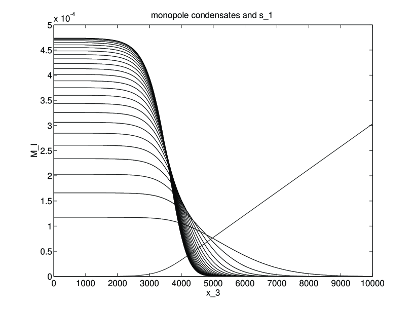
Figure 2: First approximation to the transition region of the domain wall, between the electric confinement phase on the left and the Coulomb phase on the right. One can see how the monopole condensates disappear towards the middle of the wall (the right side of the picture), while the $s^{1}$ coordinate moves from 0 up to $\frac{\pi}{2}$ at the center (far right, out of the frame). The horizontal axis is $x_{3}$ in units of $1/\Lambda$, shifted so that the zero point is deep in the confining phase on the left. The scale for the monopole condensates is shown on the left; the scale of $s^{1}$ is 2500 times large, thus $s^{1}=0.75$ at the right edge of the frame.

Given small enough $m$, equations (23–24) can be easily solved numerically. Figure (2) displays the resulting field profiles through the transition region of the wall, as calculated for $N=51$, $m=2.2\cdot 10^{-9}$. Note different monopole condensates decreasing at different rates but all reaching negligible values in the Coulomb domain (the right side of the figure).

3.2 Correcting the Trajectory: Minimizing the Energy

The net energy density of a BPS-saturated domain wall comprises potential and kinetic terms, each contributing $|\Delta W|$ to the total. The approximately but not exactly BPS domain wall of the previous section has correct kinetic energy,

$$g_{i\bar{j}}\partial_{3}A^{i}\partial_{3}\bar{A}^{\bar{\jmath}}\ =\ g_{11}\partial_{3}t^{1}\partial_{3}t^{*1}\ +\sum_{l}\left(\partial_{3}M_{l}\partial_{3}{M}_{l}^{*}+\partial_{3}\tilde{M}_{l}\partial_{3}\tilde{M}_{l}^{*}\right)$$

$$=\ \partial_{3}t^{1}\frac{\partial W}{\partial t^{1}}\ +\sum_{l}\left(\partial_{3}M_{l}\frac{\partial W}{\partial M_{l}}+\partial_{3}\tilde{M}_{l}\frac{\partial W}{\partial\tilde{M}_{l}}\right)$$

$$=\ \partial_{3}W,$$

thus

$$\epsilon_{kin}\ =\int_{-\infty}^{\infty}\!\!dx_{3}\,\partial_{3}W\ =\ \Delta W.$$ (26)

Its potential energy however is higher than BPS because of un-satisfied BPS equations (18) for the $t^{k>1}$. Indeed,

$$\epsilon_{pot}\ = \int_{-\infty}^{\infty}\!\!dx_{3}\,g^{i\bar{\jmath}}\frac{\partial W}{\partial A_{i}}\frac{\partial W^{*}}{\partial\bar{A_{\bar{\jmath}}}}$$ (27)

$$= \int\!\!dx_{3}\,\biggl{[}\sum_{k}g^{k\bar{k}}\frac{\partial W}{\partial t^{k}}\frac{\partial W^{*}}{\partial t^{*k}}\ +\sum_{l}\left(\frac{\partial W}{\partial M_{l}}\frac{\partial W^{*}}{\partial M_{l}^{*}}\,+\,\frac{\partial W}{\partial\tilde{M}_{l}}\frac{\partial W^{*}}{\partial\tilde{M}_{l}^{*}})\right)\biggr{]}$$

$$= \int\!\!dx_{3}\,\biggl{[}\partial_{3}t^{1}\,\frac{\partial W}{\partial t^{1}}\,+\sum_{l}\left((\partial_{3}M_{l}\frac{\partial W}{\partial M_{l}}+\partial_{3}\tilde{M_{l}}\frac{\partial W}{\partial\tilde{M}_{l}}\right)\,+\sum_{k\neq 1}g^{k\bar{k}}\left|\frac{\partial W}{\partial t^{k}}\right|^{2}\biggr{]}$$

$$= {}\ \Delta W\ +\int\!\!dx_{3}\sum_{k\neq 1}g^{k\bar{k}}\left|\frac{\partial W}{\partial t^{k}}\right|^{2}.$$

Altogether, the last term in eq. (27) is the excess energy density over the BPS domain wall due to violation of some of the BPS equations. Spacewise, this excess energy comes solely from the transition region ($\partial W/\partial t^{k}=0$ in both Confining and Coulomb phases), thus our approximate solution is accurate for the Coulomb phase region — which constitutes most of the wall width and provides most of its energy in the small $m$ limit. However, the transition regions of the wall are rather interesting even when they are narrow, so we would like a better approximation to the field profiles. In particular, we need to get rid of the wrong assumption about $t^{k>1}$ and calculate their actual profiles.

To obtain such a better approximation, we minimize the wall’s net energy density as a function of its field profile. Basically, we first discretize $x_{3}$ and analytically evaluate the variational derivatives of the energy with respect to all possible lattice field variations, then numerically evolve the field configuration in the direction of the steepest energy descent. The boundary values are fixed to vacuum values at the left boundary and all fields except $t^{1}$ are zero at the right boundary. We start with the approximate wall profile obtained in the previous subsection, then evolve the lattice fields until we reach the (numeric) minimum of the wall’s energy.

Our calculations are somewhat eased by the symmetries of the superpotential (14) and hence of the exact solution to the BPS equations,

$$M_{l}\equiv\tilde{M}_{l}\equiv M_{N-l}\equiv\tilde{M}_{N-l}\quad{\rm and}\quad t^{k}\equiv 0\ \forall\,{\bf even}\ k.$$ (28)

Naturally, we hardcoded these symmetries into our minimization procedure. Also, for convenience of taking the large $N$ limit, we use rescaled moduli fields

$$s^{k}=\frac{N}{2i}(t^{k}-2\delta_{k,1})\,;$$ (29)

note consistency with the $s^{1}$ variable used in eq. (22). In terms of the independent $M_{l}(x_{3})$ and $s^{k}(x_{3})$, the energy density we need to minimize is

$$\epsilon\ =\int\!\!dx_{3}\rho$$

where

$$\rho(x_{3}) = \sum_{{\rm odd}\,k}\left\{\frac{N^{2}g_{\bar{k}k}}{4}\,(\partial_{3}s^{k})^{2}\ +\ \frac{4}{g_{\bar{k}k}}\left(\smash{\sum_{l=1}^{(N-1)/2}}M_{l}^{2}\,\sin\frac{\pi kl}{N}\ -\ \frac{N^{2}m}{2}\,\delta_{k,1}\right)^{2}\right\}\!$$ (30)

$$+\sum_{l=1}^{(N-1)/2}\left\{4\bigl{(}\partial_{3}M_{l}\bigr{)}^{2}\ +\ \frac{16}{N^{2}}\,M_{l}^{2}\left(\smash{\sum_{{\rm odd}\,k}}s^{k}\,\sin\frac{\pi kl}{N}\right)^{2}\right\}$$

and

$$g_{\bar{k}k}\ \approx\ {1\over 8\pi\sin{\pi k\over 2N}}$$ (31)

since $\mathop{\rm Re}(FG^{*})\approx 1$ in eq. (17).

The technical details of the minimization procedure being rather boring, let us simply present our results. Figure (3) depicts the monopole condensates profiles — which have not changed dramatically during the energy-minimization procedure, cf. figure (2), except their transition regions became a bit narrower. This is easily understood in terms of BPS eqs. (18–19): the additional terms involving $t^{k>1}$ moduli make for steeper decrease of the monopole fields. Figure (4) displays the moduli profiles $s^{1}$ and also $s^{3}$, $s^{5}$, etc. As expected, $s^{3},s^{5},\ldots$ vanish in the Coulomb phase on the right, but not in the transition region between the confining and the Coulomb phases. For example, at its peak in the middle of the transition region, the $s^{3}$ reaches about 18% of the value of the $s^{1}$ at the same point. For other odd $k$, the $s^{k}$ reach their peaks at about the same point, reaching a value roughly proportional to $1/k$. The reason for such behavior is the superpotential (14): for large $k$, $\sin(\pi kl/N)$ oscillates faster between positive and negative values, leaving an average of order $1/k$.

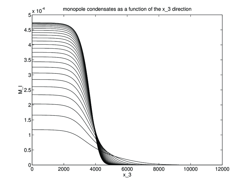
Figure 3: Field profiles for the monopoles at the final domain wall configuration, $N=51$ and $m=2.2\cdot 10^{-9}$. The highest and steepest line is $M_{25}$, and the lowest $M_{1}$.

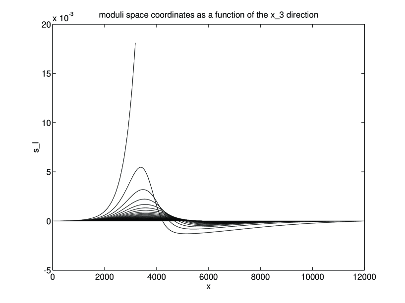
Figure 4: Field profiles for the moduli $s^{k}$ (odd $k$). The $s^{1}$ will continue to rise throughout the Coulomb but the plot is cut at $x=3200$ to avoid lines sticking out of the frame. The tallest line after $s^{1}$ is $s^{3}$, then $s^{5}$, etc.

The width of the transition region can now be measured by looking at either monopole condensates or moduli $s^{k}$. The highest peak of the $s^{3}$ field — where its value is above 50% of its maximum — corresponds to the region where the highest monopole mode $M_{(N-1)/2}$ decreases from 85% of its vacuum value down to 15%. Other monopoles are wider and recede less steeply. As for the higher moduli fields, the $s^{k>3}$ have wider peaks, for example twice as wide for $s^{21}$ than for $s^{3}$ and slightly more than that for yet larger $k$. We see no obvious way to account for this fact, other than to say that it is a numerical result. In any case, the high modes are not that much wide wider: merely by a factor of 2 rather than $N$ or even $\sqrt{N}$.

Interestingly, on the immediate right of the transition region, the $s^{k>1}$ moduli drop below zero and develop small negative values before they finally disappear in the Coulomb region. The origin of this behavior is unclear, but this is definitely not an artefact of the boundary condition. This is verified by pushing the right boundary of the lattice region further right.

Finally, we would like to mention that when all the $s^{k}$ are very small, they have comparable magnitudes, for example $s^{3}\approx 0.65s^{1}$. In other words, at the left edge of the wall, where the moduli fields just begin to shift away from their values in the confining vacuum, they move in a direction at rather wide angle to the $s^{1}$ “axis” characteristic of the Coulomb phase in the middle of the wall. This rather unexpected geometry of the wall’s ‘trajectory’ of the moduli space indicates that the present analysis does not extrapolate well into the regime of not-too-small (${\cal N}=2$)–breaking mass $m$ for which various regions of the domain wall start overlapping each other.

3.3 Conclusion

The structure of the domain wall worked out in this work is in many ways reminiscent of the $SU(2)$ domain wall. Both exhibit a similar five-layer profile, and both depend strongly on the smallness of the perturbation mass parameter $m$. The devil is in the details and the $SU(N)$ theories exhibit many new features associated with multiple monopole/dyon condensates and multiple moduli fields. There are many more BPS equations now, all entangled with each other, so calculating the field profiles of the wall calls for numerical lattice calculations. Even the BPS route that the moduli fields take on their way from one stable vacua to another is highly turns out to be non-trivial. In the $SU(N)$ model, the route between two vacua in the moduli space is not trivial, and distinct functions describe the evolutions of different monopole fields.

The large $N$ approximation helps us to get explicit expressions for the Kähler metric and for the superpotential, but unfortunately, at the end of the day we are again faced with the same limitation as in the $SU(2)$ domain wall, namely that the wall is valid only for a small perturbation parameter $m$. In fact, the limitation here is more severe, as $m$ must be smaller than ${\cal O}(N^{-4})$. For such small $m$, the five-layer picture is adequate. The work shows that the dominant field in the Coulomb phase is $t^{1}$, and the other fields either asymptote to zero, or remain very small. It is not possible, however, to disregard the other $t$’s in the transition region. As $m$ gets larger and the two transition regions overlap, on top of the difficulty from having coexisting monopole fields from two different vacua, we cannot even say along what route in the moduli space of the ${\cal N}=2$ theory the domain wall lies. The wall derived here, however, is a legitimate domain wall, and it may be interesting to study its low energy excitations in the future.

Acknowledgement: Research supported in part by the US–Israeli Binational Science Foundation, the Israeli Science Foundation, the German–Israeli Foundation for Scientific Research (GIF), the US National Science Foundation (grants PHY–95–11632 and PHY–00–71512) and the Robert A. Welsh Foundation.

References

- [1] M.R. Douglas and S.H. Shenker, Nucl. Phys. B 447 (1995) 271-296 [hep-th/9503163].
- [2] A. Kovner and M. Shifman, Phys. Rev. D56 (1997) 2396-2402 [hep-th/9611213].
- [3] G. Dvali and M. Shifman, Phys. Lett. B 396 (1997) 64-69 and ibid 407B (1997) 452 [hep-th/9612128].
- [4] A. Kovner, M. Shifman and A. Smilga, Phys. Rev. D56 (1997) 7978 [hep-th/9706089].
- [5] A.V. Smilga and A.I. Veselov, Phys. Rev. Let. 79 (1997) 4529-4532 [hep-th/9706217], Nucl. Phys. B515 (1998) 163-183 [hep-th/9710123] and Phys. Lett. 428B (1998) 303-309 [hep-th/9801142]; also A. Smilga, Phys. Rev. D58 (1998)65 [hep-th/9711032].
- [6] M. Shifman, Phys. Rev. D57 (1998) 1258-1265 [hep-th/9708060].
- [7] M. Shifman and M. Voloshin, Phys. Rev. D57 (1998) 2590-2598 [hep-th/9709137].
- [8] I.I. Kogan, A. Kovner and M. Shifman, Phys. Rev. D57 (1998) 5195-5213 [hep-th/9712046].
- [9] T. Matsuda, Phys. Lett. 436B (1998) 264 [hep-th/9805134].
- [10] K. Holland, A. Campos and U.J. Wiese, Phys. Rev. Lett. 81 (1998) 2420-2423 [hep-th/9805086].
- [11] M. Shifman, Published in Continous Advances in QCD 1998: Proceedings. Edited by A.V. Smilga. Singapore, World Scientific, 1998. pp. 526-535 hep-th/9807166.
- [12] A.V. Smilga, hep-th/9807203.
- [13] G. Dvali, G. Gabadadze and Z. Kakushadze, Nucl. Phys. B562 (1999) 158-180 [hep-th/9901132].
- [14] B. de Carlos and J.M. Moreno, Phys. Rev. Lett. 83 (1999) 2120-2123 [hep-th/9905165], and hep-th/9910208.
- [15] G. Gabadadze and M. Shifman, Phys. Rev. D61 (2000) 0750 14 [hep-th/9910050].
- [16] G. Veneziano and S. Yankielowicz, Phys. Lett. 113B (1982) 231.
- [17] T.R. Taylor, G. Veneziano and S. Yankielowicz, Nucl. Phys. B218 (1983) 493.
- [18] I. Affleck, M. Dine and N. Seiberg, Nucl. Phys. B241 (1984) 493 and Nucl. Phys. B256 (1985) 557.
- [19] V.S. Kaplunovsky, J. Sonnenschein and S. Yankielowicz, Nucl. Phys. B 552 (1999) 209-245.
- [20] N. Seiberg and E. Witten, Nucl. Phys. B 426 (1994) 19-52[hep-th/9407087] and ibid B430 (1994) 485-486.
- [21] N. Seiberg, Phys. Lett. B 206 (1998) 75.
- [22] E. Witten and D. Olive, Phys. Lett. B 78 (1978) 97.
- [23] G. Dvali and M. Shifman, Nucl. Phys. B 504 (1997) 127-146 [hep-th/9611213].
- [24] P.C. Argyres and A.E. Faraggi, Phys. Rev. Lett. 74(20) (1995) 3931-3934.
- [25] A. Klemm, W. Lerche, S. Yankielowicz and S. Theisen, Phys. Lett. B 344 (1995) 169-175.