Regularization-independent studies of nonperturbative field theory

Abstract

We propose a regularization-independent method for studying a renormalizable field theory nonperturbatively through its Dyson-Schwinger equations. Using QED₄ as an example, we show how the coupled equations determining the nonperturbative fermion and photon propagators can be written entirely in terms of renormalized quantities, which renders the equations manifestly finite in a regularization-independent manner. As an illustration of the technique, we apply it to a study of the fermion propagator in quenched QED₄ with the Curtis-Pennington electron-photon vertex. At large momenta the mass function, and hence the anomalous mass dimension $\gamma_{m}(\alpha)$, is calculated analytically and we find excellent agreement with previous work. Finally, we show that for the CP vertex the perturbation expansion of $\gamma_{m}(\alpha)$ has a finite radius of convergence.

I Introduction

As is well known, in studies of renormalizable relativistic field theories it is unavoidable to make use of a regulator in order to control the UV divergences of the theory, even though at the end this regulator is removed in order to obtain physical results. In perturbation theory the regulator and its removal via the renormalization procedure is usually little more than an inconvenience, however in nonperturbative studies, which are largely numerical, much effort needs to made in order to perform this removal in a well-controlled manner.

The best known example of the latter, of course, is lattice gauge theory[1] where the regulator is the lattice spacing and its removal entails a careful numerical extrapolation to the continuum. Another popular tool, which is the subject of this investigation, is the numerical study of a truncated set of the Dyson-Schwinger equations of the theory [2, 3, 4], where most often the regulator is simply a hard momentum cutoff $\Lambda$. Although these calculations are numerically far less demanding than the numerical integration of a functional integral, they are not entirely trivial either as they involve solving a set of integral equations for momenta $p$ ranging over many orders of magnitude, from $|p|=0$ to $|p|=\Lambda$. Renormalization then requires a further numerical extrapolation, with fixed boundary conditions provided by the relevant renormalization scheme, to $\Lambda\rightarrow\infty$.

That this removal of the regulator can be done numerically was demonstrated explicitly in Refs.[5, 6, 7] within subtractively renormalized quenched QED, using an off-shell renormalization scheme. However, as emphasized in those works and pointed out first by Dong, Munczek and Roberts [8] (it was also apparently realized at an earlier stage by Pennington [9]), the use of a momentum cut-off as a regulator is not entirely satisfactory as it violates translational invariance (in momentum space) which leads to a violation of gauge invariance in the final results, even after $\Lambda$ is taken to infinity. More precisely, this violation of gauge invariance was observed in quenched QED calculations employing the Curtis-Pennington (CP) electron-photon vertex and may be traced back to a certain, logarithmically divergent, 4-dimensional momentum integral which vanishes because of rotational symmetry at all $\Lambda<\infty$, but leads to a finite contribution for $\Lambda\rightarrow\infty$. It is this discontinuous behaviour as a function of $\Lambda$ which complicates correct numerical renormalization with this regulator. Incorrect results will be obtained unless care is taken to drop ‘gauge covariance violating terms’. Although this recipe appears to work in practise (see the Appendix of Ref. [6] as well as Ref. [10] for a more detailed discussion) it is fair to say that it is ad hoc and it would be more desirable to avoid it altogether.

Dimensional regularization, of course, does not break translational invariance and hence will not lead to the spurious gauge covariance violations outlined above. However, as shown in Ref. [11], the use of this regulator in nonperturbative studies of chiral symmetry breaking introduces a new unwelcome feature: In a dimensionally regulated theory a fermion mass will be generated dynamically at all values of the coupling constant $\alpha$ in $D\neq 4$ dimensions for any vertex which only does so above a finite critical coupling $\alpha_{cr}$ in $D=4$ dimensions. In other words, again discontinuous behaviour (this time as a function of $4-D$) prevents a naive removal of the regulator. Ultimately, it is this feature which limited the accuracy with which one could determine the critical coupling associated with the CP vertex within dimensional regularization in Ref. [11]. In addition, of course, with this regulator the integration range now extends to $|p|\rightarrow\infty$, compounding the numerical difficulties mentioned at the start. In short, although it was shown in Ref. [11] that the results obtained within dimensional regularization agree with those obtained by employing a cut-off within some limited precision, the numerical difficulties encountered in implementing this regulator has limited its further use.

It is the purpose of this letter to point out that all the difficulties mentioned above may be circumvented by removing the regulator analytically rather than numerically. This may be done by formulating the Dyson-Schwinger equations in terms of renormalized quantities only, where the dependence on the mass scale introduced by the regulator is traded for the momentum scale $\mu$ at which the theory is renormalized before performing any numerical calculations. This way dimensional regularization (or any other regulator which doesn’t violate gauge covariance) can be used and, more importantly from a numerical point of view, removal of the regulator means that no longer does one have to solve integral equations involving mass scales of vastly different orders of magnitude (and then, in addition, take a limit in which one of the scales goes to infinity). Rather, the important scales in the problem become scales of ‘physical’ importance, such as the renormalized mass $M_{\mu}$ and the renormalization scale $\mu$ at which this mass is defined. It is therefore to be expected that the dominant contributions to any integrands will be from a relatively small region of momenta. This feature is generic; i.e. it is independent of the particular vertex Ansatz that one makes use of and it remains a valid consideration for an arbitrary renormalizable field theory. Hence, although we shall illustrate this approach only within QED (and numerically only within quenched QED), it is our hope that ultimately this ‘regularization-free’ approach will prove its utility elsewhere.

To a certain extent there is a price to be paid for using the approach advocated above: one looses all contact to the bare theory. In particular, we stress that because of this one cannot study dynamical chiral symmetry breaking in this approach by simply setting the bare mass $m_{0}$ equal to zero and investigating at what point a dynamical fermion mass is generated. It is in this crucial point that we differ from the analysis in Ref. [13] where, within quenched QED, a removal of the regulator was attempted in a manner which has some similarity to what we do here. Indeed, as emphasized particularly by Miranksy (Refs. [14], [2] as well as Ch 10.7 of Ref. [3]), some care needs to be taken with the treatment of the bare mass while removing the regulator in order to avoid drawing incorrect conclusions about the presence or absence of dynamical chiral symmetry breaking in gauge theories. In the present approach this problem is avoided: chiral symmetry breaking, both explicit as well as dynamical, is characterized by a nonzero renormalized mass $M_{\mu}$, and hence this quantity in itself does not distinguish between these two possibilities. In Section III, we shall take (within quenched QED) the somewhat more indirect signal of the appearance of oscillations in the renormalized fermion mass function [14] as an indicator of the onset of dynamical chiral symmetry breaking.

This paper is organized as follows: in the next section all reference to the bare Lagrangian will be explicitly eliminated by re-expressing the Dyson-Schwinger equations of full QED in terms of renormalized quantities only. As a first application of this seemingly innocuous step we then re-examine, in the second part of this paper, the large momentum behaviour of the electron propagator in quenched QED₄ (employing the Curtis-Pennington vertex [12]). In particular, because of the absence of a cut-off, scaling invariance in this momentum region is restored in the equation for the electron’s mass function and hence this equation can be solved analytically. We compare the results with existing numerical studies and also use it to derive the analytic form of the anomalous mass dimension $\gamma_{m}(\alpha)$ within this offshell momentum subtraction scheme. Finally, we discuss the analytic behaviour of $\gamma_{m}(\alpha)$ as a function of the coupling and conclude.

II Regularization-independent formulation

The Dyson-Schwinger equations for the renormalized electron and photon propagators (Fig. 1) are well known. For example, employing dimensional regularization, we have

$$S^{-1}(\mu;p) = Z_{2}(\mu){S^{0}}^{-1}(p)\>-\>iZ_{1}(\mu){e_{\mu}}^{2}\int{d^{D}k\over(2\pi)^{D}}\>\Gamma^{\alpha}(\mu;p,k)\>S(\mu;k)\gamma^{\beta}\>D_{\alpha\beta}(\mu;q)$$ (1)

$$\equiv Z_{2}(\mu){S^{0}}^{-1}(p)\>-\>Z_{1}(\mu)\>\bar{\Sigma}(p)$$ (2)

$$D_{\alpha\beta}^{-1}(\mu;q) = Z_{3}(\mu){D_{\alpha\beta}^{0}}^{-1}(q)\>+\>iZ_{1}(\mu){e_{\mu}}^{2}N_{F}\>{\rm tr}\int{d^{D}k\over(2\pi)^{D}}\>\Gamma_{\alpha}(\mu;p,k)\>S(\mu;k)\>\gamma_{\beta}\>S(\mu;p)\>$$ (3)

$$\equiv Z_{3}(\mu){D_{\alpha\beta}^{0}}^{-1}(q)\>+\>Z_{1}(\mu)\>\bar{\Pi}_{\alpha\beta}(q)$$ (4)

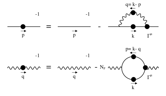
FIG. 1.: The Dyson-Schwinger equations for the fermion and photon propagators in QED

Here $N_{F}$ is the number of species of fermions in the theory and the constants $Z_{1}(\mu)$, $Z_{2}(\mu)$ and $Z_{3}(\mu)$ are the vertex, fermion wave function and photon wave function renormalization constants, respectively. We have assumed, for convenience, that the $N_{f}$ fermions are identical (i.e. they have equal mass), the generalization being straightforward. $S(\mu;p)$ and $D_{\alpha\beta}(\mu;q)$ are the full fermion and photon propagators renormalized at the momentum scale $\mu$ ($S^{0}(p)$ and $D_{\alpha\beta}^{0}(q)$ are their bare counterparts), while the full (proper) fermion-photon vertex is $\Gamma_{\alpha}(\mu;k,p)$. These propagators are usually expressed in terms of scalar functions $Z(\mu^{2};p^{2})$, $M(p^{2})$ and $G(\mu^{2};q^{2})$ through

$$S(\mu;p)\>=\>\frac{Z(\mu^{2};p^{2})}{\not\!p-M(p^{2})}\hskip 42.67912ptD_{\alpha\beta}(\mu;q)\>=\>-\frac{1}{q^{2}}\,\left[G(\mu^{2};q^{2})\left(g_{\alpha\beta}-\frac{q_{\alpha}q_{\beta}}{q^{2}}\right)+\xi\frac{q_{\alpha}q_{\beta}}{q^{2}}\right],$$ (5)

where $\xi$ is the renormalized covariant gauge fixing parameter, so that the fermion’s equation separates into two scalar equations

$$Z^{-1}(\mu^{2};p^{2}) = Z_{2}(\mu)\>-\>Z_{1}(\mu)\>\bar{\Sigma}_{d}(p^{2})$$ (6)

$$M(p^{2})\>Z^{-1}(\mu^{2};p^{2}) = Z_{2}(\mu)\>m_{0}\>+\>Z_{1}(\mu)\>\bar{\Sigma}_{s}(p^{2})\;\;\;.$$ (7)

Here $\bar{\Sigma}_{d}(p^{2})$ and $\bar{\Sigma}_{s}(p^{2})$ refer, respectively, to the Dirac odd and even parts of $\bar{\Sigma}(p)$, i.e. $\bar{\Sigma}(p)=\not\!p\;\bar{\Sigma}_{d}(p^{2})+\bar{\Sigma}_{s}(p^{2})$. The bar over these quantities indicates that we have explicitly separated out the renormalization constants $Z_{i}(\mu)$; also, note that we do not indicate the implicit dependence of $\bar{\Sigma}_{d,s}(p^{2})$, through the functions $Z(\mu^{2};p^{2})$ and $D_{\alpha\beta}(\mu;q)$, on $\mu^{2}$. The equivalent equation for the photon wavefunction renormalization $G(\mu^{2};q^{2})$ is given by

$$G^{-1}(\mu^{2};q^{2})\>=\>Z_{3}(\mu)\>+\>Z_{1}(\mu)\>\bar{\Pi}(q^{2})\;\;\;,$$ (8)

where $\bar{\Pi}^{\alpha\beta}(q)\equiv-q^{2}\left(g^{\alpha\beta}-\frac{q^{\alpha}q^{\beta}}{q^{2}}\right)\bar{\Pi}(q^{2})$. Note that, as we are free to use a regulator which respects gauge covariance and will use a vertex which satisfies the Ward-Takahashi identity, $\bar{\Pi}^{\alpha\beta}(q)$ does not contain spurious quadratic divergences [15] and is transverse as it should be. Hence the term involving the gauge parameter $\xi$ on the left hand side of Eq. (3) precisely cancels the corresponding term involving $\xi_{0}$ in $D_{\alpha\beta}^{0}$ on the right hand side (i.e. $\xi_{0}=Z_{3}\xi$).

The renormalization constants $Z_{i}(\mu)$ as well as $m_{0}$ are fixed by the boundary conditions

$$Z(\mu^{2};\mu^{2})\>=\>1\quad\quad\quad M(\mu^{2})\>\equiv\>M_{\mu}\quad\quad\quad G(\mu^{2};\mu^{2})\>=\>1\;\;\;.$$ (9)

(Although we shall not do so here, in practice the fermion and photon can be renormalized at two different scales $\mu^{2}$ and ${\mu^{\prime}}^{2}$. In QED it is usual to choose the latter as ${\mu^{\prime}}^{2}=0$, in which case ${e_{\mu^{\prime}}}^{2}/(4\pi)$ just becomes the physically measured fine structure constant $\alpha$.) Because of the Ward-Takahashi identity, which should be satisfied by the vertex Ansatz for $\Gamma_{\alpha}$, one has $Z_{1}(\mu)=Z_{2}(\mu)$.

In order to avoid cumbersome notation, we have not explicitly indicated functional dependence on the regulator in Eqs. (1)–(8). Most of the above quantities, i.e. $Z(\mu^{2};p^{2})$, $M(p^{2})$ and $G(\mu^{2};q^{2})$, as well as $Z_{1,2,3}(\mu)$, are functions of the regulator. Indeed, if one keeps $M_{\mu}$ and $e_{\mu}$ fixed as one removes the regulator, which is the standard textbook prescription, the bare fermion mass $m_{0}$ and the bare charge also become regulator dependent.

As one removes the regulator, the integrals on the right hand side of Eqs. (1) and (3), and hence $\bar{\Sigma}_{d}(p^{2})$, $\bar{\Sigma}_{s}(p^{2})$ and $\bar{\Pi}(q^{2})$ diverge logarithmically (or, to be more precise, in dimensional regularization they develop singularities at $D=4$). It is the defining feature of a renormalizable field theory that these divergences may be absorbed into the constants $Z_{1,2,3}(\mu)$ and into the bare mass $m_{0}$, rendering finite limits for $Z(\mu^{2};p^{2})$, $M(p^{2})$ and $G(\mu^{2};q^{2})$. However, we can make use of the $p^{2}$ independence of $Z_{1,2,3}(\mu)$ and $m_{0}$ in order to eliminate these constants from the above equations. For example, by evaluating Eq. (6) at a second momentum which, for convenience, we take to be $p^{2}=\mu^{2}$, and forming an appropriate difference one obtains

$$Z(\mu^{2};p^{2})\>=\>1\>+\>Z(\mu^{2};p^{2})\>\bar{\Sigma}_{d}(p^{2})\>-\>\bar{\Sigma}_{d}(\mu^{2})$$ (10)

where we have made use of the renormalization condition (9). Because the left hand side of this equation is finite as the regulator is removed, the right hand side must also be (even though, of course, the individual terms on the RHS separately diverge). In a similar way one obtains

$$M(p^{2})\>=\>M_{\mu}\>+\>\left[M(p^{2})\bar{\Sigma}_{d}(p^{2})\>+\>\bar{\Sigma}_{s}(p^{2})\right]\>-\>\left[M_{\mu}\bar{\Sigma}_{d}(\mu^{2})\>+\>\bar{\Sigma}_{s}(\mu^{2})\right]$$ (11)

and

$$G^{-1}(\mu^{2};q^{2})\>=\>1\>+\>\left[G^{-1}(\mu^{2};q^{2})\bar{\Sigma}_{d}(\mu^{2})\>+\>\bar{\Pi}(q^{2})\right]\>-\>\left[\bar{\Sigma}_{d}(\mu^{2})\>+\>\bar{\Pi}(\mu^{2})\right]\;\;\;.$$ (12)

We note in passing that the perturbative solution of these three equations defines ‘finite QED’ in a rather different sense to that developed by Johnson, Baker and Willey [16]. We do not pursue this further here; rather, the main point of this letter is to point out that these renormalized equations (10) to (12) (with the regulator removed, of course), or equivalently their counterparts in QCD or any other renormalizable field theory, provide a starting point for nonperturbative investigations which has some significant advantages over the usual treatment found in the literature. To illustrate this we now turn to the well-studied example of quenched QED.

III Application to Quenched QED₄

For quenched QED Eq. (12) becomes irrelevant and Eqs. (10) and (11) reduce to one-dimensional integral equations. In particular, if we employ the CP vertex (which, importantly for the present approach, satisfies the Ward-Takahashi identity and respects renormalizability) and make use of a regulator which does not violate gauge covariance then these renormalized equations become, in Euclidean space,

$$Z(\mu^{2};p^{2}) = 1-\frac{\alpha\xi}{4\,\pi}\,\int_{p^{2}}^{{\mu}^{2}}dk^{2}\frac{1}{\left[k^{2}+M^{2}(k^{2})\right]}\,Z(\mu^{2};k^{2})$$ (14)

$$\hskip 42.67912pt+\frac{\alpha}{4\,\pi}\,\int_{0}^{\infty}\frac{dk^{2}}{\left[k^{2}+M^{2}(k^{2})\right]}\left[Z(\mu^{2};p^{2})\,I(k^{2},p^{2})\>-\>I(k^{2},\mu^{2})\right]$$

$$M(p^{2}) = M_{\mu}+\frac{\alpha}{4\pi}\int_{0}^{\infty}\frac{dk^{2}}{\left[k^{2}+M^{2}(k^{2})\right]}\left[J(k^{2},p^{2})-J(k^{2},\mu^{2})\right.$$ (16)

$$\left.\hskip 142.26378pt\>+\>M(p^{2})\>I(k^{2},p^{2})-M_{\mu}\>I(k^{2},\mu^{2})\right]$$

where $I(k^{2},p^{2})$ and $J(k^{2},p^{2})$ are those of Table. 1 of Atkinson et al.’s paper [17], apart from the term proportional to $\xi\left(1+{M^{2}(k^{2})\over k^{2}}\right)$ in $I(k^{2},p^{2})$ in their paper which originated from the violation of gauge covariance by their cutoff mentioned in the introduction. As promised, these equations are finite in the absence of a regulator. The equation for the wavefunction renormalization function (Eq. 14) is the same as Eq. (10) in Ref. [13], however our treatment of the mass function differs from theirs. We shall not solve these equations numerically here but, rather, shall make use of the fact that, for momenta $k^{2}$ larger than $M^{2}(k^{2})$, the absence of a cut-off implies that they become scaling invariant. Hence we can solve them analytically in this region for finite $M_{\mu}$, in the same way as was done by Atkinson et al. [17] for the chirally symmetric theory (i.e. $M_{0}=M_{\mu}=0$).

A Large Momentum Behaviour in Quenched QED₄

For $k^{2}>>M^{2}(k^{2})$ Eqs. (14, 16) may be expanded in powers of ${M^{2}(k^{2})\over k^{2}}$. Keeping at most linear terms in $M(k^{2})$ we obtain

$$Z(\mu^{2};p^{2}) = 1\>-\>\frac{\alpha\xi}{4\pi}\int_{p^{2}}^{\mu^{2}}\frac{dk^{2}}{k^{2}}Z(\mu^{2};k^{2})\quad,$$ (17)

$$M(p^{2}) = M_{\mu}\>+\>{\alpha\xi\over 4\pi}\left\{\int_{0}^{p^{2}}{dk^{2}\over p^{2}}{Z(\mu^{2};k^{2})\over Z(\mu^{2};p^{2})}M(k^{2})\>-\>\int_{0}^{\mu^{2}}{dk^{2}\over\mu^{2}}Z(\mu^{2};k^{2})M(k^{2})\right\}$$ (20)

$$\>+\>{3\alpha\over 8\pi}\int_{0}^{\infty}dk^{2}\left\{\left[2\,M(k^{2}){p^{2}\over p_{>}^{2}}{{Z(\mu^{2};k^{2})\over Z(\mu^{2};p^{2})}-{k^{2}\over p^{2}}\over p^{2}-k^{2}}\right.\right.$$

$$\left.\left.\hskip 42.67912pt\>-\>{Z(\mu^{2};k^{2})\over Z(\mu^{2};p^{2})}{p_{<}^{2}\over p_{>}^{2}}{M(p^{2})-M(k^{2})\over p^{2}-k^{2}}\right]\>-\>[p^{2}\rightarrow\mu^{2}]\right\}\;\;,$$

where $p_{<}^{2}$ ($p_{>}^{2}$) is the minimum (maximum) of $p^{2}$ and $k^{2}$.

Because of scaling invariance, these equations are solved by a power law Ansatz for $Z(\mu^{2};p^{2})$ and $M(p^{2})$, i.e.

$$Z(\mu^{2};p^{2})\>=\>\left(\frac{p^{2}}{\mu^{2}}\right)^{\nu}\quad\quad M(p^{2})\>=\>M_{\mu}\left(\frac{p^{2}}{\mu^{2}}\right)^{-s}\;\;\;.$$ (21)

The reader should note that the overall scale of $M(p^{2})$ is fixed by the renormalization condition. Explicitly, one finds $\nu$ and $s$ to be given by

$$\nu=\frac{\alpha\xi}{4\pi}\quad,$$ (22)

$$\frac{3\nu}{2\xi}\Bigg{[}2\pi\cot{s\pi}-\pi\cot{\nu\pi}+3\pi\cot(\nu-s)\pi+\frac{2}{(1-s)}+\frac{1}{(\nu+1)}+\frac{1}{\nu}$$ (23)

$$\hskip 170.71652pt-\frac{3}{(\nu-s)}-\frac{1}{(\nu-s+1)}\Bigg{]}+\frac{s-1}{\nu-s+1}=0\quad.$$ (24)

These are the same powers as those found in Ref. [17] (corrected for the gauge covariance violating term). We emphasize that in contrast to the unrenormalized equations in Ref. [17], for the renormalized equations this power Ansatz is valid whether or not the bare mass $m_{0}$ is zero. We demonstrate this explicitly in Fig. (2), where the above asymptotic form of the mass function (dashed line) is compared to previously published numerical work (Ref. [6]) with $m_{0}\neq 0$ (solid line). As one can see there is excellent agreement in the region $p^{2}>>M^{2}(p^{2})$. Quantitatively, one sees in Table [1] that the logarithmic slope $s$ calculated from Eq. (24) for a variety of gauge parameters and couplings agrees, in most cases, with the same quantity extracted from the published numerical work to better than 1 part in $10^{5}$.

We note that in the above calculations $\alpha<\alpha_{cr}$. There are, in general, several real solutions $s$ to Eq. (24) at these values of the coupling (see also Ref. [17]). However, only one of these matches smoothly onto the perturbative solution and it is this one which is used above. The other solution appears to be a spurious byproduct of the linearized approximation (20) to Eq. (16) (Solutions which do not match smoothly onto perturbation theory can arise in Eq. (20) if the integrals diverge like ${1\over\alpha}$ due to IR divergences; this cannot occur in the exact Eq. (16) because of the regulating mass in the denominator). Because $s$ is real there are no oscillations in the mass function and hence there is no chiral symmetry breaking for these couplings. For $\alpha>\alpha_{cr}$, however, the solutions $s$ become complex. As Eq. (24) defines $s$ as a real analytic function of $\alpha$, it is clear that if $s$ is a solution, then so is $s^{*}$. In this case the correct asymptotic tail to the oscillating, but real, mass function (Eq. 16) is obtained by a suitable superposition of these two particular solutions to Eq. (20). The oscillations are the indication that, above $\alpha_{cr}$, chiral symmetry is broken in quenched QED employing the CP vertex.

         

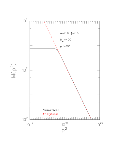
FIG. 2.: Comparison of a numerical solution for the mass function $M(p^{2})$ (solid line, obtained from Ref. [6]) and the analytical expectation for its asymptotic behaviour (dashed line, Eq. 24). The renormalized mass is $M_{\mu}=400$ (arbitrary units), while $\alpha=0.6$ and $\xi=0.5$.

B The anomalous mass dimension

The analytical expression for the asymptotic behaviour of the mass function is closely related to the anomalous mass dimension of the theory, i.e.

$$\gamma_{m}\>=\>{d\log Z_{m}\over d\log\mu}\>\rightarrow\>2s\;\;\;,$$ (25)

where we have used $Z_{m}\equiv m_{0}/M_{\mu}$ and the asymptotic form of the mass function in Eq. (20). Hence Eq. (24) defines, within the off-shell renormalization scheme used here, the prediction for the asymptotic value of the anomalous mass dimension obtained with the CP vertex as a function of the coupling and the gauge parameter $\xi$. For convenience, let us restrict ourselves to Landau gauge, in which case one obtains

$$\alpha\>=\>-\frac{8}{3}\frac{1}{\left[\cot\left(\frac{\pi\>\gamma_{m}}{2}\right)+\frac{1}{\pi}\frac{\gamma_{m}^{2}\>+\>2\>\gamma_{m}\>-\>12}{\gamma_{m}(2\>-\>\gamma_{m})}\right]}\;\;\;.$$ (26)

It is amusing to note the similarity of this equation, obtained within the framework of Dyson-Schwinger equation studies, to that obtained for the anomalous mass dimension within the MS scheme using a completely different nonperturbative approach [18], namely one based on the use of a variational principle for the evaluation of the functional integral, i.e.

$$\alpha\>=\>{4\over 3}\left(1+\gamma_{m}^{\rm var}\right)\cot\left({\pi\over 2}\>{1\over 1+\gamma_{m}^{\rm var}}\right)\;\;\;.$$ (27)

Not only are both equations implicit equations for $\gamma_{m}$, but even the same transcendental function is involved in both. Actually, the similarity does not end there. It is a simple matter to numerically solve Eq. (26) for complex $\alpha$ in order to investigate its analytic structure. The result, for both the imaginary and real part of the anomalous mass dimension, is shown in Fig. (3). A branch point in $\alpha$ is clearly visible on the positive real axis (the direction of the cut is arbitrary). Its position may be determined via a bifurcation analysis of Eq. (24) or, equivalently, Eq. (26). Its numerical value is $\alpha=0.933667$ (in Feynman gauge it is $\alpha=0.890712$) and it coincides, of course, with the well-known critical coupling associated with the CP vertex [17, 11] above which the theory breaks chiral symmetry. The variational result for the same quantity in the MS scheme, Eq. (27), also results in a branch point, however this time it is at a complex value of $\alpha$ [18, 19]. Hence no sign of chiral symmetry breaking for $\alpha>\alpha_{cr}$ was seen in $\gamma_{m}^{\rm var}$ in that work.

 

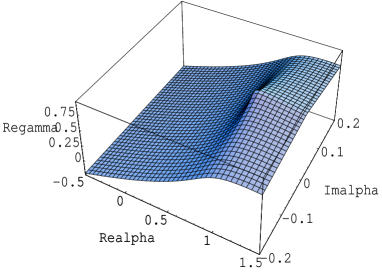
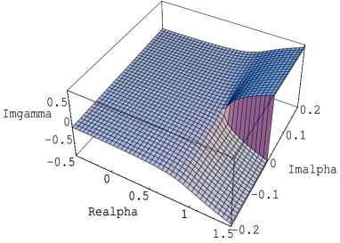
FIG. 3.: The real and imaginary part of the anomalous mass dimension versus complex coupling constant.

Apart from the presence of a branch point at finite $\alpha$, the other notable feature in Fig. (3) (also found for $\gamma_{m}^{\rm var}(\alpha)$ in Refs. [18, 19]) is the absence of a branch point, or any other nontrivial analytic structure, at $\alpha=0$, i.e. the radius of convergence of the perturbation expansion of $\gamma_{m}(\alpha)$ as obtained with the CP vertex is finite. This is in marked contrast to general expectations from studies of high order perturbation theory [20], where the factorial growth in the number of diagrams results in a vanishing of the radius of convergence of the perturbation expansion of a general Green function. It is difficult to specify whether or not the CP vertex correctly reproduces the factorial growth in the number of diagrams. What can be said with certainty, however, is that clearly the Dyson-Schwinger equation for the fermion propagator does not itself generate a branch point at $\alpha=0$ like it does, for example, at $\alpha=\alpha_{cr}$. If a branch point at $\alpha=0$ is present in the exact theory then it already needs to be present in the vertex itself.

Finally, associated with the above analytical structure, one can derive the behaviour of high order perturbation theory for $\gamma_{m}(\alpha)$ from Eq. (26), using the methods discussed in [19]. We define the expansion coefficients $c_{n}$ through

$$\gamma_{m}(a) = \sum_{n=1}^{\infty}c_{n}\>a^{n}\quad\quad\quad a\equiv{\alpha\over\pi}$$ (28)

so that the radius of convergence (in $a$) is given by $\lim_{n\rightarrow\infty}|c_{n}|^{-1/n}$. The asymptotic behaviour of these coefficients may be derived most easily by converting Eq. (24) into a differential equation:

$$-\frac{8}{3a^{2}}=\frac{1}{2}\left\{\pi^{2}+\left[-\frac{8}{3a}+1+3f(a)+g(a)\right]^{2}\right\}{\gamma_{m}^{\prime}(a)}+3f^{\prime}(a)+g^{\prime}(a)$$ (29)

where we have defined $f(a)=2/{\gamma_{m}(a)}$ and $g(a)=1/[1-\gamma_{m}(a)/2]$. These functions have the perturbative expansions

$$f(a)=\frac{2}{a\,c_{1}}\sum_{n=0}^{\infty}b_{n}\>a^{n}\quad\quad g(a)=\sum_{n=0}^{\infty}d_{n}\>a^{n}$$ (30)

where the coefficients $b_{n}$ and $d_{n}$ are related to the $c_{n}$’s through [21]

$$b_{0}\>=\>1\quad d_{0}\>=\>1$$ (31)

$$b_{n}\>=\>-\sum_{k=1}^{n}b_{n-k}{c_{k+1}\over c_{1}}\quad d_{n}\>=\>{1\over 2}\sum_{k=1}^{n}d_{n-k}\>c_{k}\quad\quad\quad n>0$$ (32)

These equations, together with Eqs. (28) and (30) substituted into Eq. (29), define the expansion coefficients $c_{n}$ and may be solved iteratively to very high orders. For the first few orders we obtain

$$\gamma_{m}(\alpha) = \frac{3}{2}\frac{\alpha}{\pi}+\frac{9}{8}\left(\frac{\alpha}{\pi}\right)^{2}+\frac{9}{64}(9+\pi^{2})\left(\frac{\alpha}{\pi}\right)^{3}$$ (34)

$$\hskip 14.22636pt+\frac{81}{256}(6+\pi^{2})\left(\frac{\alpha}{\pi}\right)^{4}+\frac{81}{2560}(105+20\pi^{2}+\pi^{4})\left(\frac{\alpha}{\pi}\right)^{5}+{\cal{O}}(\alpha^{6})$$

while for large $n$ the behaviour of the coefficients approaches the form

$$c_{n}=\left({\alpha_{cr}\over\pi}\right)^{-n}\frac{e^{-\beta_{0}}}{n^{3/2}}$$ (35)

with $\beta_{0}\approx 0.52$. The absence of a term of the form $n^{n}$ indicates the absence of factorial growth mentioned previously and the power $3/2$ in the denominator is indicative of the fact that close to the branch point the cut has the character of a square root.

IV Conclusions and Outlook

In this letter we have argued that there are significant advantages in performing nonperturbative calculations based on the use of Dyson-Schwinger equations in a manner different to that commonly used in the literature. The central idea is to work with renormalized quantities only, allowing one to completely eliminate the regulator. Within QED, this allows one to avoid spurious problems associated with the usual cut-off regulator, such as the breaking of gauge covariance in the fermion propagator and the introduction of unwanted quadratic divergences into the photon propagator. Furthermore we have shown that, within quenched QED, it allows one to gain an analytical understanding of both the mass function at large momenta as well as the analytic structure of the anomalous mass dimension of this theory. We expect that the main advantage of the method, however, will be that one can restrict the numerical task of solving the Dyson-Schwinger equations of any renormalizable theory to a relatively small region of momenta. For example, we anticipate that this feature will make it feasible to study full, rather than quenched, QED₄. Furthermore, it is our hope that the numerical task of solving a coupled set of Dyson-Schwinger equations is sufficiently simplified by the approach discussed here to allow one to consider pushing the truncation of this set beyond the equations for the two-point functions.

- [1] H. J. Rothe, Lattice Gauge Theories: an Introduction, (World Scientific, Singapore, 1992).
- [2] P. I. Fomin, V. P. Gusynin, V. A. Miransky and Yu. A. Sitenko, Riv. Nuovo Cim. 6 (1983) 1.
- [3] V. A. Miransky, Dynamical Symmetry Breaking in Quantum Field Theories, (World Scientific, Singapore, 1993).
- [4] C.D. Roberts and A.G. Williams, Prog. Part. Nuc. Phys. 33 (1994) 477.
- [5] F.T. Hawes and A.G. Williams, Phys. Rev. D 51 (1995) 3081.
- [6] F.T. Hawes, A.G. Williams and C.D. Roberts, Phys. Rev. D 54 (1996) 5361.
- [7] F.T. Hawes, T. Sizer and A.G. Williams, Phys. Rev. D 55 (1997) 3866.
- [8] Z. Dong, H. Munczek, and C. D. Roberts, Phys. Lett. 333B (1994) 536.
- [9] See Footnote 1 in A. Bashir and M. R. Pennington, Phys. Rev. D 50 (1994) 7679.
- [10] A. Kızılersü, T. Sizer and A. G. Williams, ADP-99-43-T380, hep-ph/0001147.
- [11] A.W. Schreiber, T. Sizer and A.G. Williams, Phys. Rev. D 58 (1998) 125014 ; V. P. Gusynin, A. W. Schreiber, T. Sizer and A.G. Williams, Phys. Rev. D 60 (1999) 065007.
- [12] D.C. Curtis and M.R. Pennington, Phys. Rev. D 42 (1990) 4165 and references therein.
- [13] D.C. Curtis and M.R. Pennington, Phys. Rev. D 46 (1992) 2663.
- [14] V. A. Miransky, Phys. Lett. 165B (1985) 401; ibid, Il Nuovo Cim. 90A (1985) 149; see also D. Atkinson and P. W. Johnson, Phys. Rev. D35 (1987) 1943.
- [15] K.-I. Kondo, H. Mino and H. Nakatani, Mod. Phys. Lett. A17 (1992) 1509; J. C. R. Bloch and M.R. Pennington, Mod. Phys. Lett. A10 (1995) 1225.
- [16] K. Johnson, M. Baker and R. Willey, Phys. Rev. 136 (1964) B1111.
- [17] D. Atkinson et al., Phys. Lett. 329B (1994) 117.
- [18] C. Alexandrou, R. Rosenfelder and A.W. Schreiber, Phys. Rev. D 62 (2000) 085009.
- [19] A.W. Schreiber, R. Rosenfelder and C. Alexandrou, in “Proceedings of the 3rd International Symposium on Symmetries in Subatomic Physics”, eds. X.-H. Guo and A. W. Thomas, to be published by AIP Conference Proceedings, ADP-00-20 /T403, hep-th/0007182.
- [20] L. N. Lipatov, Sov. Phys. JETP 45 (1977) 216; for a review, see E. Bogomol’nyi, V. A. Fateev and L. N. Lipatov, Physics Reviews 2 (1980) 247 as well as the collection of papers in “Large-order behaviour of perturbation theory”, eds. J.C. Le Guillou and J. Zinn-Justin, North-Holland (1990).
- [21] I. S. Gradshteyn and I. M. Ryzhik: Table of integrals, series and products, 4th edition, Academic Press (1980), p. 14.