HAMILTONIAN SOLUTION OF THE SCHWINGER MODEL WITH COMPACT U(1)

Abstract

We present the complete exact solution of the Schwinger model with compact gauge group $U(1)$ (compact case). This is realized by demanding that the true electromagnetic degree of freedom $c$ has angular character. This is suggested by the loop approach to this problem and defines a version of the Schwinger model which is different from the standard one, where the electromagnetic degree of freedom ultimately takes values on the line (non-compact case). All our results follow naturally from the compactification condition. The main consequences are: the spectra of the zero modes is not degenerated and does not correspond to the equally spaced harmonic oscillator, the spectra and wave functions of the excited states also differ from those of the standard case, both the electric charge and a modified gauge invariant chiral charge are conserved and, finally, there is no need to introduce a $\theta$-vacuum. Nevertheless, the axial-current anomaly is still present. In more detail, these unusual properties turn out to be a consequence of the following basic features: (i) the compactification condition makes the electromagnetic degree of freedom $c$ invariant under small and large gauge transformations. (ii) this full gauge invariance is inherited by the fermionic creation and annihilation operators, which are subsequently used to solve the model and (iii) the boundary conditions upon the wave functions,which are imposed by demanding hermiticity of both the electric field and the zero mode Hamiltonian, in the compact space of the variable $c$. They result in requiring the wave functions $F(c)$ (and their first derivatives) to be equal at points $\pm\,{\bar{c}}$, corresponding to the beginning and the end of the circle $-\,{\bar{c}}<\,c\,<\,{\bar{c}}$. These end points must be identified as a single physical point in the compact electromagnetic configuration space. A comparison with the standard Schwinger model is pointed out along the text.

I Introduction

One of the most popular exactly soluble systems in quantum field theory is the Schwinger model, which describes electrodynamics in $1+1$ dimensions [1]. This model has been solved in many ways and we have not attempted here to provide a complete list of all the related references [2, 3, 4, 5, 6, 7, 8, 9, 10].

Most of the solutions consider the one dimensional coordinate space as a line or a circle, with the basic electromagnetic degree of freedom, the zero mode of the spatial component of the electromagnetic potential $A_{1}$, taking values in the interval $[-\infty,+\infty]$. We refer to this version of the model as the non-compact case, where the topological qualification refers, from now on, to the electromagnetic configuration variables and not to the space coordinates.

In general, gauge theories have also their compact version, which is realized when the degrees of freedom corresponding to the gauge field take values on a compact interval. The natural settings for this to happen are, on one hand, the lattice formulation of gauge theories [11] and on the other, the loop-space formulation of gauge theories [12]. In the latter approach, all the information about the theory is encoded in terms of variables which are invariant under small and large gauge transformations. In $1+1$ dimensions the basic variable for the electromagnetic degrees of freedom is $\exp[ie\int_{0}^{L}dxA_{1}(x)]$ and, consequently, the loop representation naturally describes compact electrodynamics, since it is enough to restrict $c={1\over L}\int_{0}^{L}dxA_{1}(x)$ to the interval $\{-{\pi\over eL},{\pi\over eL}\}$ [13]. The loop representation can also encompass the non-compact case, at the expense of introducing additional degrees of freedom [14].

As emphasized by Polyakov [15], the selection of one type of theory (compact case) over the other (non-compact case) has to be decided only on empirical grounds according to the predictions of each choice. From a more technical point of view we can say that compact gauge theories are blind to large gauge transformations, while non-compact ones have to be supplemented by $\theta$-vacua in order to preserve the invariance under such transformations. One also expects that one of the main differences between the compact and the non-compact cases would show up in the boundary conditions satisfied by the corresponding wave functionals, rather than in the specific form of the (functional) differential equations describing the dynamics . This is in complete analogy with the simple case of a one-dimensional particle in a line ( non-compact situation) versus the one dimensional rigid rotator (compact situation)[16], which are both described by the same Schroedinger equation, but subjected to different boundary conditions.

Many solutions to the standard Schwinger model, $c$ in the line $\{-\infty,+\infty\}$, start from considering $c$ as an angular variable. Nevertheless, using appropriate boundary conditions, the corresponding authors manage to unfold the circle into the line, i.e. to go from compact $U(1)$ to its universal covering [5, 7, 8, 9].

In this work we maintain the angular character of $c$ and fully explore the consequences of this choice which, up to our knowledge, are not previously reported in the literature. It is important to emphasize that our results follow uniquely from the compactification condition, together with the standard definitions of both a scalar product and the hermiticity conditions in the corresponding Hilbert space. Not surprisingly, the compactification prescription leads to a model which drastically differs from the NCSM, as will be seen along the text.

The compactification of the gauge group $U(1)$ is realized by demanding that the only surviving electromagnetic degree of freedom $c$ behaves as an angular variable living in a circle of length $\frac{2\,\pi}{eL}$. In the sequel we call this model the compact Schwinger model, or the compact case. Furthermore, we are going to take full advantage of one of the many methods which have been successfully applied previously to solve the non-compact model. To this purpose we have selected the Hamiltonian approach of Refs. [8, 9] upon which the present work heavily relies.

In the present Hamiltonian formulation we obtain the complete solution of the compact Schwinger model, including the ground and excited states. A partial solution of the CSM was found in Ref. [13], using the loop approach to this problem [12], and served as motivation for the work presented here. These partial results coincide with those obtained in this work. Previous progress in the solution of this model were reported in [17].

The possibility of rewriting the initially linear fermionic Hamiltonian in terms of the corresponding Sugawara currents [18], together with the introduction of the Bogoliubov transformation in the Hamiltonian approach are the fundamental keys to obtain the full solution of the model. The formulation of these topics in the loop approach provides an interesting subject for future studies.

The paper is organized as follows: Section II contains a brief motivation for our compactification procedure, arising from the loop approach quantization of the free electromagnetic field. In Section III we define the compact Schwinger model and state our notation and conventions. In Section IV we discuss the gauge invariance of the model. There it is shown how the compactification condition, i.e. our choice for the topology of $c$, leads to fully gauge invariant electromagnetic and fermionic degrees of freedom, which are subsequently used in the resolution of the model. We also consider the Gauss law and show that it implies that the physical states of the theory must be independent of the excited modes of the electromagnetic potential. In section V we construct the fermionic Fock space in a background electromagnetic field and introduce the total electric charge $Q$ together with the total modified chiral charge $\bar{Q}_{5}$. Both charges are gauge invariant and conserved, in contrast with the non-compact case where $\bar{Q}_{5}$ is not fully gauge invariant. In Section VI we perform the full quantization of the model. Using a Bogoliubov transformation we get a complete solution for the ground and excited states. In Section VII we present a detailed proof of the conservation of the modified chiral charge ${\bar{Q}}_{5}$. Accordingly, we show that there is no spontaneous symmetry braking, since the fermionic condensates $\langle\bar{\psi}\psi\rangle$ and $\langle\bar{\psi}\gamma_{5}\psi\rangle$ are exactly zero. In consequence, the $\theta$-vacuum structure is not required in the compact Schwinger model. We summarize our results in Section VIII, emphasizing the main differences with the standard Schwinger model. The Appendix contains the calculation of the regularized current algebra of the model, together with the corresponding hermiticity properties.

II Motivation

In this section we provide a motivation for the compactification of the electromagnetic degree of freedom in the framework of the loop-space formulation of the free electromagnetic field. We take the space as a circle of length $L$ and impose periodic boundary conditions on $A_{\mu}$.

Classically, our choice of gauges is $A_{0}=0$, together with $\partial_{1}A_{1}=0$. This implies $A_{1}=A_{1}(t)=c(t)$, leaving the zero mode of the electromagnetic potential as the only true electromagnetic degree of freedom, with $E={\dot{c}}$. We still have the freedom of large gauge transformations $A_{\mu}\rightarrow A_{\mu}-\partial_{\mu}\,\alpha,\ \alpha=\frac{2\,\pi\,n}{e\,L}\,x$, which change

$$c(t)\rightarrow c(t)-\frac{2\,\pi\,n}{e\,L}\,$$ (1)

leaving $A_{0}=0$ together with $E$ invariant.

The quantization is performed in the subspace $A_{0}=0=\Pi_{0}$, and subsequently imposing the remaining Gauss law constraint upon the physical states. The Hamiltonian density, the Gauss law and the commutation relations are

$${\cal H}=\frac{1}{2}\,E^{2},\qquad{\cal G}=\partial_{x}\,E\approx 0,\qquad[A_{1}(x),\,E(y)]=i\,\hbar\,\delta(x-y),$$ (2)

Expanding in modes, we have

$$A_{1}(x,t)=c(t)+\sum_{m\neq 0}A_{m}\,{\rm exp}\left(\frac{2\,\pi\,m}{L}\,x\right),$$ (3)

$$E(x,t)=E_{0}(t)+\sum_{m\neq 0}E_{m}\,{\rm exp}\left(-\frac{2\,\pi\,m}{L}\,x\right),\qquad E^{2}=\sum_{m\geq 0}E_{m}^{*}\,E_{m},$$ (4)

leading to

$$[A_{m},\,E_{n}]=\frac{i\,\hbar}{L}\,\delta_{mn}\quad\Rightarrow\qquad[{c}(t),\,{E}_{0}(t)]=\frac{i\,\hbar}{L}.$$ (5)

In the connection representation we have the realization $E_{n}=\frac{i\,\hbar}{L}\frac{\partial}{\partial\,A_{n}}$ for the above commutators. Only the zero-mode survives because the Gauss law implies $E_{m}=0,m\neq 0$, upon the physical states. That is to say $\Psi_{\rm phys}=\Psi(c)$. The Hamiltonian is

$$H=-\frac{\hbar^{2}}{2L}\frac{d^{2}}{d\,c^{2}},$$ (6)

with the corresponding eigenfunctions and eigenvalues

$$\Psi(c)=\Psi_{0}\,{\rm exp}(i\,p\,c),\qquad E_{p}=\frac{\hbar^{2}\,p^{2}}{2\,L}$$ (7)

The precise nature of the spectra will depend on the boundary conditions imposed upon the wave functions.

Now we turn to the loop approach, where we introduce

$$T^{0}[\gamma]={\rm exp}\left(i\,e\,\oint_{\gamma}d\,x\,A_{1}(x,t)\right)={\rm exp}\left(i\,e\,c(t)\,M\,L\right),$$ (8)

as the manifestly gauge invariant electromagnetic degree of freedom. Here $M=0,\,\pm\,1,\,\pm\,2\dots$ is the number of turns of the loop $\gamma$, which completely characterize any loop in our spatial circle. In fact, $T^{0}[\gamma]$ is also invariant under large gauge transformations, because

$$T^{0}[\gamma]\rightarrow{\rm exp}\left(i\,e\,M\,L\,\left(c(t)-\frac{2\,\pi\,n}{e\,L}\right)\right)={\rm exp}\left(i\,M\,n\,2\pi\right)T^{0}[\gamma]=T^{0}[\gamma].$$ (9)

Let us consider the gauge invariant operators ${\hat{T}}^{0}[N]$ and ${\hat{E}}$, such that

$${\hat{T}}^{0}[N]={\rm exp}\left(i\,e\,{\hat{c}}\,N\,L\right),\quad[{\hat{T}}^{0}[N],\,{\hat{E}}]=-\,e\,\hbar\,N\,{\hat{T}}^{0}[N].$$ (10)

The Hilbert space $\{|N\rangle\}$, where the states are labeled by the number of turns, is built by starting from the vacuum $|0\rangle$

$${\hat{E}}\,|0\rangle=0,\qquad|N\rangle={\hat{T}}^{0}[N]\,|0\rangle,$$ (11)

where we have

$$|N+P\rangle={\hat{T}}^{0}[N]\,|P\rangle,\quad{\hat{E}}\,|N\rangle=\,e\,N\,|N\rangle.$$ (12)

The Hamiltonian is

$$H=\int_{0}^{L}d\,x\frac{1}{2}E^{2},\qquad H\,|N\rangle=\frac{1}{2}(\,e^{2}\,\hbar^{2}\,L)\,N^{2}\,|N\rangle=(\,\hbar\,e^{2}\,L^{2})\,\frac{\hbar}{2\,L}\,N^{2}\,|N\rangle.$$ (13)

Here, the choice of boundary conditions, which determine the eigenvalues and eigenfunctions, is somewhat hidden in the algebraic process. In order to make them explicit, we introduce a modified connection representation basis $|{\tilde{c}}\rangle$ defined by

$$|{\tilde{c}}\rangle=\sum_{N}\,{\rm exp}(i\,e\,{\tilde{c}}\,N\,L)\,|N\rangle=\sum_{N}\,{\rm exp}\left(i\frac{\pi{\tilde{c}}}{{\bar{c}}}N\right)\,|N\rangle,\qquad\quad{\bar{c}}=\frac{\pi}{e\,L},$$ (14)

which is a superposition of fully gauge invariant states. From the above expression we verify that $|{\tilde{c}}+2\,M\,{\bar{c}}\rangle\,=\,|{\tilde{c}}\rangle$, which states the angular character of the variable ${\tilde{c}}$ in an interval of length $2\,{\bar{c}}$, which we choose to be $-{\bar{c}}\leq{\tilde{c}}\leq{\bar{c}}$.

The inversion of the above relation is

$$|N\rangle=\int_{-{\bar{c}}}^{{\bar{c}}}d\,{\tilde{c}}\,\,{\rm exp}\left(-i\frac{\pi{\tilde{c}}}{{\bar{c}}}\,N\right)\,|{\tilde{c}}\rangle.$$ (15)

Summarizing, in the modified connection representation with ${\tilde{c}}$ being the angular variable defined above, we have the following realization for the operators

$${\hat{E}}=\frac{\hbar}{i\,L}\frac{\partial}{\partial{\tilde{c}}},\qquad H=-\frac{\hbar^{2}}{2L}\frac{\partial^{2}}{\partial{\tilde{c}}^{2}},$$ (16)

together with the corresponding eigenfunctions, and its derivatives

$$\Psi_{N}({\tilde{c}})=\frac{1}{\sqrt{2\,{\bar{c}}}}\,{\rm exp}\left(-i\frac{\pi{\tilde{c}}}{{\bar{c}}}\,N\right),\qquad\frac{d\,\Psi_{N}({\tilde{c}})}{d\,{\tilde{c}}}=-\frac{i\,\pi\,N}{\sqrt{2\,{\bar{c}}^{3}}}\,{\rm exp}\left(-i\frac{\pi{\tilde{c}}}{{\bar{c}}}\,N\right).$$ (17)

Clearly the above functions satisfy the boundary conditions

$$\Psi_{N}|_{{\tilde{c}}=-{\bar{c}}}=\Psi_{N}|_{{\tilde{c}}=+{\bar{c}}},\qquad\frac{d\,\Psi_{N}}{d\,{\tilde{c}}}|_{{\tilde{c}}=-{\bar{c}}}=\frac{d\,\Psi_{N}}{d\,{\tilde{c}}}|_{{\tilde{c}}=+{\bar{c}}}.$$ (18)

From now on we will denote by $c$ the compacted variable ${\tilde{c}}$.

III The model

In the sequel we use similar notation and conventions as those in Ref.[9]. The model is described by the Lagrangian

$${\cal L}=-\frac{1}{4}F_{\mu\nu}F^{\mu\nu}+\bar{\psi}\gamma^{\mu}\left(i\partial_{\mu}-eA_{\mu}\right)\psi$$ (19)

where $F_{\mu\nu}=\partial_{\mu}A_{\nu}-\partial_{\nu}A_{\mu}$, $\bar{\psi}=\psi^{\dagger}\gamma^{0}$ is a Grassmann valued fermionic field and we are using units such that $\hbar=c=1$. We consider the coordinate space to be $S^{1}$ and we will require periodic(antiperiodic) boundary conditions for the fields

$$A_{\mu}(x+L)=A_{\mu}(x),\quad\psi(x+L)=-\psi(x),$$ (20)

where $L$ is the length of the circle. The gamma matrices are: $\gamma^{0}=\sigma_{1},\;\gamma^{1}=i\sigma_{2},\;\gamma^{5}=-\gamma^{0}\gamma^{1}=\sigma_{3}$, where $\sigma_{i}$ are the standard Pauli matrices. We use the signature $(+,-),\;\;i.e.\;\;\eta_{00}=-\eta_{11}=1$.

After the standard canonical analysis of the Lagrangian density (19), describing the configuration space variables $A_{0},\,A_{1}$ and $\psi$, we obtain

$${\cal H}=\frac{1}{2}E^{2}+i\psi^{\dagger}\sigma_{3}\left(\partial_{1}+ieA_{1}\right)\psi-A_{0}\,\left(\partial_{1}\,E-e\,\psi^{\dagger}\,\psi\right),\qquad\Pi_{0}\approx 0,$$ (21)

where the corresponding canonical momenta are $\Pi_{0},\,\Pi_{1}=F_{01}=E$ and $\Pi_{\psi}=-i\,\psi^{*}$. Conservation in time of the primary constraint $\Pi_{0}\approx 0$ leads to the Gauss law constraint

$${\cal G}=\partial_{1}E-e\psi^{\dagger}\psi\approx 0.$$ (22)

There are no additional constraints.

At this stage we partially fix the gauge in the electromagnetic potential by choosing

$$A_{0}=0,\quad\Pi_{0}=0.$$ (23)

The only remaining constraint ${\cal G}$ is first class and it will be imposed strongly upon the physical states of the system.

From now on we use the notation $A_{1}=A$ for the surviving electromagnetic degree of freedom. Also we have $\psi=(\psi_{1},\psi_{2})^{\top}$, where $\top$ denotes transposition. The charge density is given by $\rho(x)=e\psi^{\dagger}\psi=e(\psi_{1}^{*}\psi_{1}+\psi_{2}^{*}\psi_{2}$). The resulting Poisson brackets algebra at equal times is

$$\left\{A(x),E(y)\right\}=\delta(x,y),\qquad\left\{\psi_{\eta}(x),\psi^{*}_{\xi}(y)\right\}=-i\delta_{\eta\xi}\delta(x,y),\quad\eta,\xi=1,2\,,$$ (24)

with all other brackets being zero.

The standard canonical quantization procedure leads to the following non-zero commutators $(\hbar=1)$

$$\left[A(x),E(y)\right]=i\delta(x,y),\qquad\left\{\psi_{\eta}(x),\psi^{*}_{\xi}(y)\right\}=\delta_{\eta\xi}\delta(x,y).$$ (25)

The gauge chosen in (23) does not completely fix the electromagnetic degrees of freedom, leaving the Lagrangian density (19) still invariant under the following gauge transformations

$$\psi\rightarrow{\rm e}^{ie\alpha(x)}\psi,\quad A_{\mu}\rightarrow A_{\mu}-\partial_{\mu}\alpha(x),$$ (26)

generated by the remaining Gauss law constraint. The constant piece $\alpha_{0}$ of the function $\alpha(x)$ is irrelevant in the above transformation. In the sequel we consider ${\bar{\alpha}}(x)=\alpha(x)-\alpha_{0}$ as the function generating the gauge transformations. Notice that $\partial_{0}\alpha(x)=0$ respects the gauge condition $A_{0}=0$.

There are two families of gauge transformations:

1. Those continuously connected to the identity, called small gauge transformations (SGT), characterized by the function

   $${\bar{\alpha}}(x)=b\left(e^{i2\pi nx/L}-1\right),$$ (27)

   which is periodic in $x$ and preserves the boundary conditions (20).

2. The second family corresponds to the so called large gauge transformations (LGT), which are generated by the non-periodic functions

   $${\bar{\alpha}}(x)={2\pi n\over eL}x=2\,n{\bar{c}}\,x,\quad n=\pm 1,\pm 2,\dots.$$ (28)

   The boundary conditions (20) are also preserved in this case.

Notice that in both cases we have

$${\bar{\alpha}}(0)=0.$$ (29)

At this stage we define the compact Schwinger model by demanding that the only true degree of freedom arising from the electromagnetic potential in one dimension, which is the zero mode $c$, be restricted to the interval

$$-{\bar{c}}\leq\,c=\frac{1}{L}\int_{0}^{L}A(z)\,dz\,\leq{\bar{c}}.$$ (30)

In the previous section we provided some motivation for considering this situation.

Equation (30) means that two values of $c$ differing by $2\,{\bar{c}}\,N=\frac{2\,\pi\,N}{eL}$ must be identified as a single physical point in the compact space of the variable $c$.

Since the remaining electromagnetic degrees of freedom are pure gauge, we expect the possible compactification of them to be irrelevant. Nevertheless, there still remains the question of in which way, if any, the imposed compactification shows itself in the fermionic degrees of freedom of the problem. These topic will be addressed to in the next section.

IV Identification of the gauge invariant degrees of freedom

Let us consider the following Fourier decomposition for the electromagnetic potential $A(x)$, the field strength $E(x)$ and the gauge transformation function ${\bar{\alpha}(x)}$

$$A(x) = c+\sum_{m\neq 0}A_{m}\ {\rm e}^{\frac{2\pi im}{L}x},\quad E(x)=E_{0}+\sum_{m\neq 0}E_{m}\ {\rm e}^{-\frac{2\pi im}{L}x},$$ (31)

$${\bar{\alpha}}(x) = \sum_{m\neq 0}{\bar{\alpha}}_{m}\ {\rm e}^{\frac{2\pi im}{L}x},$$ (32)

leading to the following inverse transformations

$$c=\frac{1}{L}\int_{0}^{L}dx\ A(x),\quad A_{m}=\frac{1}{L}\int_{0}^{L}dx\ A(x)\ {\rm e}^{-\frac{2\pi im}{L}x},\ m\neq 0,$$ (33)

with similar expressions for $E_{0},E_{m},{\bar{\alpha}}_{m}$. Let us observe that $E_{m}^{\dagger}=E_{-m}$, $A_{m}^{\dagger}=A_{-m}$ in virtue of the hermiticity of both $E(x)$ and $A(x)$. Let us remark that

$$0={\bar{\alpha}}(0)=\sum_{m\neq 0}{\bar{\alpha}}_{m},$$ (34)

which will be used in the sequel.

Under a gauge transformation $A(x)\rightarrow A(x)-\frac{\partial{\bar{\alpha}}(x)}{\partial x}$, the corresponding modes change as

$$c\rightarrow c-\frac{1}{L}({\bar{\alpha}}(L)-{\bar{\alpha}}(0)),\quad A_{m}\rightarrow A_{m}-\frac{2\pi im}{L}\ {\bar{\alpha}}_{m},\quad m\neq 0.$$ (35)

Clearly, the zero mode $c$ is invariant under the small gauge transformations generated by ${\bar{\alpha}}=b\left({\rm e}^{i2\pi nx/L}-1\right)$. As for the LGT (28), $c\rightarrow c-\frac{2\pi n}{eL}$, but these points must be identified, according to the compactification condition (30). In other words, $c$ is also invariant under large gauge transformations.

Summarizing, the zero mode $c$ is fully gauge invariant.

The remaining electromagnetic modes $A_{m}$ are decoupled from the theory due to the Gauss Law (22), as will be shown below.

Next we consider the expansion of the fermionic variables in a background electromagnetic field. According to Ref. [9], these can be written as

$$\psi_{1}(x,t)=\sum_{n}a_{n}\phi_{n}(x){\rm e}^{-i\epsilon_{n}t},\quad\psi_{2}(x,t)=\sum_{n}b_{n}\phi_{n}(x){\rm e}^{i\epsilon_{n}t},$$ (36)

where $a_{n},b_{n}$ are standard fermionic annihilation operators satisfying the non-zero anticommutators

$$\{a_{m},a_{n}^{\dagger}\}=\delta_{mn},\quad\{a_{m},a_{n}\}=0,\quad\{b_{m},b_{n}^{\dagger}\}=\delta_{mn},\quad\{b_{m},b_{n}\}=0,$$ (37)

while any of the $a$’s anticommutes with any of the $b$’s. The states $\psi_{1}\ (\psi_{2})$ describe the positive  (negative) chiral (eigenvalues of $\gamma_{5}$) sectors of the model.

The basic functions $\phi_{n}$ , together with the eigenvalues of the energy are given by

$$\phi_{n}(x)={1\over\sqrt{L}}e^{-i\epsilon_{n}x-ie\int_{0}^{x}A(z)dz},\quad\epsilon_{n}={2\pi\over L}\left(n+{1\over 2}-{eL\over 2\pi}c\right)\equiv{2\pi n\over L}+{\pi\over L}-ec.$$ (38)

Rewriting the fermionic sector of the Hamiltonian density (21) as ${\cal H}_{F}=\psi^{\dagger}h_{F}\psi$, we observe that the corresponding eigenvalues of $h_{F}$ are $+\epsilon_{n}$ and $-\epsilon_{n}$ for the positive and negative quirality sectors, respectively.

Since $c$ is invariant under large and small gauge transformations the energy eigenvalues $\epsilon_{n}$ are fully gauge invariant. Furthermore, according to the definition (38)

$$\phi_{n}\to{\rm e}^{ie\,\bar{\alpha}(x)}\phi_{n},$$ (39)

under gauge transformations, where we have used $\bar{\alpha}(x)=0$ which is valid for both large and small gauge transformations. As a consequence of the above properties and in order to recover the transformation law (26) of the fermionic field $\psi$, we must have

$$a_{n}\rightarrow a_{n},\quad b_{n}\rightarrow b_{n}.$$ (40)

for the gauge transformation of the fermionic operators $a_{n}$ and $b_{n}$. In other words, consistency among the compactification condition (30), the transformation law (26) and the definition (38) demands that the basic fermionic operators $a_{n}$ and $b_{n}$ are fully gauge invariant in the compact case.

Let us emphasize that the above property establishes a main difference between the compact and the non-compact cases. Following the same steps in the latter situation we obtain that the change $c\rightarrow c-\frac{2\pi n}{eL}$, under large gauge transformations and with these points not identified, implies that the energy eigenvalues are not gauge invariant, i.e. $\epsilon_{n}\to\epsilon_{n+1}$, which leads to $\phi_{n}(x)\to{\rm e}^{-ie\bar{\alpha}(x)}\phi_{n+1}$. Then, in order to satisfy the transformation property (26) of the fermionic field, we must have now that $a_{n}\rightarrow a_{n+1},b_{n}\rightarrow b_{n+1}$, under LGT.That is to say, the fermionic operators are not fully gauge invariant in the non-compact case.

In this way, it is transparent that the topological behavior of $c$, i.e. compact versus non-compact variable, implies a completely different transformation law for the fermionic operators $a_{n},b_{n}$ under gauge transformations.

Using the Fourier expansions (31) and (36), we rewrite the commutators for the fields in terms of the corresponding modes. In particular, the commutator $[E(x),\psi_{\alpha}(y)]=0$ leads to

$$[E_{m},a_{n}]=\frac{ie}{2\pi m}\left(a_{n}-a_{n+m}\right),\ \ m\neq 0,\qquad[E_{0},a_{n}]=0,$$ (41)

$$[E_{m},b_{n}]=\frac{ie}{2\pi m}\left(b_{n}-b_{n+m}\right),\ \ m\neq 0,\qquad[E_{0},b_{n}]=0.$$ (42)

The remaining commutators are

$$[A_{k},A_{l}]=0=[E_{k},E_{l}],\quad[A_{k},E_{l}]=\frac{i}{L}\delta_{kl},\quad[A_{k},a_{n}]=0,\quad[A_{k},b_{m}]=0.$$ (43)

Next, we concentrate on the commutator algebra of the Fourier modes. To this end, we introduce the following operators

$$j_{++}^{nm}=a_{n}^{\dagger}a_{m},\hskip 28.45274ptj_{--}^{nm}=b_{n}^{\dagger}b_{m},\hskip 28.45274ptj_{+-}^{nm}=a_{n}^{\dagger}b_{m},\hskip 28.45274ptj_{-+}^{nm}=b_{n}^{\dagger}a_{m},$$ (44)

which satisfy $(j_{++}^{nm})^{\dagger}=j_{++}^{mn},\ (j_{--}^{nm})^{\dagger}=j_{--}^{mn}$   and   $(j_{+-}^{mn})^{\dagger}=j_{-+}^{nm}$. Additional useful combinations of the above fermionic operators are the currents

$$j_{+}(x)=\psi_{1}{}^{\dagger}(x)\psi_{1}(x)=\frac{1}{L}\sum_{n=-\infty}^{+\infty}{\rm e}^{-\frac{2\pi in}{L}x}\ j_{+}{}^{n},$$ (45)

$$j_{-}(x)=\psi_{2}{}^{\dagger}(x)\psi_{2}(x)=\frac{1}{L}\sum_{n=-\infty}^{+\infty}{\rm e}^{+\frac{2\pi in}{L}x}\ j_{-}{}^{n},$$ (46)

where

$$j_{+}{}^{n}=\sum_{m=-\infty}^{\infty}j_{++}^{m,m+n},\quad j_{+}{}^{0}=Q_{+},\qquad j_{-}{}^{n}=\sum_{m=-\infty}^{\infty}j_{--}^{m+n,m},\quad j_{-}{}^{0}=Q_{-}.$$ (47)

At this stage we introduce the $\zeta-$regularized form of the currents defined in Eq.(47),

$$j_{+}{}^{n}|_{\rm reg}={\rm lim}_{s\rightarrow 0}\sum_{m=-\infty}^{\infty}\frac{1}{\lambda_{m,s}}a^{\dagger}_{m}a_{m+n},\quad j_{-}{}^{n}|_{\rm reg}={\rm lim}_{s\rightarrow 0}\sum_{m=-\infty}^{\infty}\frac{1}{\lambda_{m,s}}b^{\dagger}_{m+n}b_{m}.$$ (48)

In the sequel we will drop the subindex $|_{\rm reg}$ from the above currents, but we will always consider their form (48) in calculating any relation involving them. At the end of the calculation we will take the $s\rightarrow 0$ limit. In other words, we will construct an algebra among regularized objects, which will be further restricted to the action upon the physical Hilbert space of the problem.

As it is shown in detail the Appendix, the regularized current algebra of the operators (48) is given by

$$[j_{+}{}^{n},(j_{+}{}^{m})^{\dagger}]=n\delta_{m,n},\qquad[j_{-}{}^{n},(j_{-}{}^{m})^{\dagger}]=n\delta_{m,n},\qquad[j_{+}{}^{n},j_{-}{}^{m}]=0.$$ (49)

The above commutation relations are the same as those obtained in the non-compact case. The calculation here is somewhat different than the one in Ref. [9] because we have used the regularized expressions (48) for the currents. We have also verified in the Appendix that the regularized currents satisfy the hermiticity properties

$$(j_{\pm}{}^{m})^{\dagger}=j_{\pm}{}^{-m}.$$ (50)

In order to satisfy the commutation relations (41) and (42) we make the ansatz

$$E_{m}=\frac{1}{iL}\frac{\partial}{\partial A_{m}}-\frac{e}{2\pi im}\left(j_{+}{}^{m}+(j_{-}{}^{m})^{\dagger}\right),\ \ m\neq 0,\quad E_{0}=\frac{1}{iL}\frac{\partial}{\partial c},$$ (51)

which clearly satisfies the third commutation relation in (43). Let us emphasize that the fields $E_{m},\ m\neq 0$, defined in Eq.(51) satisfy also the second commutation relation in (43), by virtue of (49). Substituting the expressions (51) in the corresponding commutators of Eq.(41) we obtain

$$\frac{\partial a_{n}}{\partial A_{m}}=-\frac{eL}{2\pi m}a_{n},\ m\neq 0,\quad\frac{\partial a_{n}}{\partial c}=0.$$ (52)

The above equation leads to the following solution for the fermionic operators with respect to their dependence on the gauge field

$$a_{m}={\rm exp}\left(-\frac{eL}{2\pi}\sum_{k\neq 0}\frac{1}{k}A_{k}\right){\bar{a}}_{m}\equiv U{\bar{a}}_{m},$$ (53)

where ${\bar{a}}_{m}$ are new fermionic operators which are independent of the gauge field $A_{k}$ and which also satisfy the basic fermionic anticommutation relations. In fact, the transformation $U$ defined above is unitary because $A_{k}{}^{\dagger}=A_{-k}$. A relation analogous to (53) can be found for the remaining fermionic operators: $b_{m}=U{\bar{b}}_{m}$, where the new operators $\bar{b}_{m}$ are independent of the electromagnetic potential by construction.

The expression (53) reproduces the fully gauge invariant character of $a_{n}$. In fact, under the gauge transformation given by (35), the exponential in (53) changes by a factor ${\rm exp}(ie\sum_{k\neq 0}{\bar{\alpha}}_{k})$ which is exactly ${\rm exp}(ie{\bar{\alpha}}(0))=1$, according to the relation (34). The same result is obtained for the operators $b_{n}$.

With the ansatz (51), the Gauss law ${\cal G}(x)=-\frac{1}{L}\sum{\rm exp}(-\frac{2\pi imx}{L}){\cal G}_{m}$ reduces to

$${\cal G}_{0} = e\left(j_{+}{}^{0}+(j_{-}{}^{0})^{\dagger}\right)=eQ$$ (54)

$${\cal G}_{m} = 2\pi im\ E_{m}+e\left(j_{+}{}^{m}+(j_{-}{}^{m})^{\dagger}\right)=\frac{2\pi m}{L}\frac{\partial}{\partial A_{m}},\quad m\neq 0.$$ (55)

These expressions reproduce the transformation property

$$[{\cal G}(x),a_{n}]=ea_{n}\delta(x)\Longleftrightarrow[{\cal G}_{m},a_{n}]=-e\ a_{n},$$ (56)

in virtue of the relation (52). The above commutator is the infinitesimal version of the relation (40).

Our expression (54) for the Gauss law constraint is somewhat different from the one obtained in Ref. [9]. Imposing this constraint upon the physical states we conclude that the wave functions of the system must be of zero electric charge and also independent of the modes $A_{m},\ m\neq 0$, which explicitly show the decoupling of the $m\neq 0$ electromagnetic modes.

In particular, the following bilinears in the fermionic operators: $a^{\dagger}a,\,a^{\dagger}b,\,b^{\dagger}a,\,b^{\dagger}b$, which will be subsequently used in the solution of the model, are independent of the electromagnetic modes and are gauge invariant under SGT and LGT.

Summarizing, we have shown that the compactification condition (30) implies that the operators $c$, $a_{n}$ and $b_{n}$ are fully gauge invariant. Also, the Gauss constraint imply that the wave function of the system is independent of the electromagnetic modes $A_{m},\ m\neq 0$.

V Fock Space

We now construct the fermionic Fock space in a background electromagnetic field. Starting from the vacuum $|0\rangle$ annihilated by the operators $a_{n}$ (positive quirality sector), $b_{n}$ (negative quirality sector), the Dirac vacuum $|vac\rangle$ is constructed in such a way that all negative energy levels are filled. Our compactification condition (30) for the electromagnetic variable $c$ implies that all levels with $n\leq-1\ (n\geq 0)$ have negative energies for the positive  (negative) quirality sectors, respectively. In this way, the Dirac vacuum is

$$|vac\rangle=\prod_{n=-\infty}^{-1}a_{n}^{\dagger}|0\rangle\otimes\prod_{n=0}^{\infty}b_{n}^{\dagger}|0\rangle.$$ (57)

The $\zeta-$regularized Hamiltonians and the $\zeta-$regularized charge operators of the positive (negative) chiral sectors are given by [9]

$$H_{+} = \lim_{s\rightarrow 0}\sum_{n\in Z}\frac{\epsilon_{n}}{\lambda_{n,s}}a_{n}^{\dagger}a_{n}{\hskip 28.45274pt}Q_{+}=\lim_{s\rightarrow 0}\sum_{n\in Z}\frac{1}{\lambda_{n,s}}a_{n}^{\dagger}a_{n}$$ (58)

$$H_{-} = \lim_{s\rightarrow 0}\sum_{n\in Z}\frac{(-\epsilon_{n})}{\lambda_{n,s}}b_{n}^{\dagger}b_{n}{\hskip 28.45274pt}Q_{-}=\lim_{s\rightarrow 0}\sum_{n\in Z}\frac{1}{\lambda_{n,s}}b_{n}^{\dagger}b_{n},$$ (59)

where the regulator is given by $\lambda_{n,s}=|\lambda\,\epsilon_{n}|^{s}$, with $\lambda$ been a parameter with dimensions of inverse energy.

The total charge $Q$, the total chiral charge $Q_{5}$ and the total energy $H$ are hermitian operators defined by

$$Q=Q_{+}+Q_{-},\quad Q_{5}=Q_{+}-Q_{-},\quad H_{F}=H_{+}+H_{-}.$$ (60)

The eigenvalues of the above operators for the Dirac vacuum state are

$$Q|vac\rangle = 0,\qquad Q_{5}|vac\rangle=-\frac{ecL}{\pi}|vac\rangle,$$ (61)

$$H_{F}|vac\rangle = \frac{2\pi}{L}\left\{\left(\frac{ecL}{2\pi}\right)^{2}-\frac{1}{12}\right\}|vac\rangle\equiv{\varepsilon}_{0}|vac\rangle,$$ (62)

At this level it is already convenient to introduce the modified chiral charge

$${\bar{Q}}_{5}=lim_{s\rightarrow 0}\sum_{n=-\infty}^{+\infty}\frac{1}{|\lambda\epsilon_{n}|^{s}}\left({a}_{n}^{\dagger}{a}_{n}-{b}_{n}^{\dagger}{b}_{n}\right)+\frac{ecL}{\pi},$$ (63)

which is invariant under SGT and LGT in the compact Schwinger model. This is not the case in the non-compact situation, where ${\bar{Q}}_{5}$ is not invariant under LGT. The eigenvalues of ${\bar{Q}}_{5}$ are integer numbers in the fermionic Hilbert space. In the sequel we will refer to ${\bar{Q}}_{5}$ as the (total) modified chiral charge of the system. Also, a given eigenvalue $2\,M$ of ${\bar{Q}}_{5}$ will be referred to as the $M$-chiral sector of the theory. In this way, the second equation (62) reads ${\bar{Q}}_{5}|vac\rangle=0$, which assigns zero chiral charge to the Dirac vacuum.

In order to construct excited states with different modified chiral charge, we need to use the operators (44). The application of any of them to $|vac\rangle$ produce new energy eigenstates with the same zero eigenvalue for the electric charge. Nevertheless, the chiral charge is changed in steps of two units, by the action of $j_{+-}$, $j_{-+}$.

Let us focus on the states

$$j_{+-}^{pq}|vac\rangle,\ p,q\geq 0\hskip 28.45274ptj_{-+}^{pq}|vac\rangle,\ p,q<0,$$ (64)

where the choice of $p,q$ in each case is such that a non-zero vector results. If we compute their energy, we find

$$H_{F}(j_{+-}^{pq}|vac\rangle) = ({\varepsilon}_{0}+\epsilon_{p}+\epsilon_{q})j_{+-}^{pq}|vac\rangle,$$ (65)

$$H_{F}(j_{-+}^{pq}|vac\rangle) = ({\varepsilon}_{0}-\epsilon_{p}-\epsilon_{q})j_{-+}^{pq}|vac\rangle.$$ (66)

The chiral charge of these states is

$${\bar{Q}}_{5}(j_{+-}^{pq}|vac\rangle) = \ 2j_{+-}^{pq}|vac\rangle,$$ (67)

$${\bar{Q}}_{5}(j_{-+}^{pq}|vac\rangle) = -2j_{-+}^{pq}|vac\rangle.$$ (68)

From Eqs. (66) and (68) we conclude that the state with chiral charge $+2$ and lowest energy ${\varepsilon}_{1}={\varepsilon}_{0}+2\epsilon_{0}$ is

$$j_{+-}^{00}|vac\rangle=\prod_{n=-\infty}^{0}a_{n}^{\dagger}\prod_{n=1}^{\infty}b_{n}^{\dagger}|0\rangle\equiv\left|{\varepsilon}_{1},2\right\rangle.$$ (69)

Analogously, the state with chiral charge $-2$ and lowest energy ${\varepsilon}_{-1}={\varepsilon}_{0}-2\epsilon_{-1}$ is

$$j_{-+}^{-1-1}|vac\rangle=\prod_{n=-\infty}^{-2}a_{n}^{\dagger}\prod_{n=-1}^{\infty}b_{n}^{\dagger}|0\rangle\equiv\left|{\varepsilon}_{-1},-2\right.\rangle.$$ (70)

Repeating this procedure we construct the local ground states $\left|{\varepsilon}_{N},2N\right\rangle$, for a definite quirality $2\,N,\,\ N\in{\cal Z}$,

$$j_{+-}^{NN}\left|{\varepsilon}_{N},\,2N\right\rangle = \left|{\varepsilon}_{N+1},\,2(N+1)\right\rangle,$$ (71)

$$j_{-+}^{N-1N-1}\left|{\varepsilon}_{N},\,2N\right\rangle = \left|{\varepsilon}_{N-1},\,2(N-1)\right\rangle,$$ (72)

having minimum energy ${\varepsilon}_{N},$ determined by the recursions ${\varepsilon}_{N+1}={\varepsilon}_{N}+2\epsilon_{N}$ and ${\varepsilon}_{N-1}={\varepsilon}_{N}-2\epsilon_{N-1}$, respectively. The above states can be written as

$$\left|{\varepsilon}_{N},2N\right\rangle=\prod_{n=-\infty}^{N-1}a_{n}^{\dagger}|0\rangle\otimes\prod_{m=N}^{\infty}b_{m}^{\dagger}|0\rangle.$$ (73)

Using the regularized expression for the fermionic Hamiltonian, the result

$${\varepsilon}_{N}(c)=\frac{2\pi}{L}\left\{\left(N-\frac{ecL}{2\pi}\right)^{2}-\frac{1}{12}\right\},$$ (74)

is obtained, which is equivalent to what we get using the recursions previously indicated. In the above notation the Dirac vacuum state is

$$|vac\rangle=\left|{\varepsilon}_{0},0\right\rangle.$$ (75)

All the states (73) have zero electric charge, which is not explicitly written.

Summarizing, from the Dirac vacuum we have so far constructed states with minimum energy for each possible chirality. As noticed before, each one of these states can be considered as a local vacuum in the corresponding quirality sector.

We are now in position to determine the characteristics of the complete fermionic spectrum in the electromagnetic external field. Within each chiral sector and starting from the local ground state $|{\varepsilon}_{N},2N\rangle$, we have to consider all possible zero-charge excitations generated by $a^{\dagger}_{p}a_{q}$. The corresponding minimum energy ${\varepsilon}_{N}$ will be shifted to ${\varepsilon}_{N}+\epsilon_{p}-\epsilon_{q}={\varepsilon}_{N}+\frac{2\pi}{L}(p-q)$. Furthermore, the expression (73) implies that

$$a^{\dagger}_{p}a_{q}|{\varepsilon}_{N},2N\rangle=0,\quad p<q,\quad q>N-1.$$ (76)

In this way, only the excitations with $p\geq q$ are allowed. An analogous result is obtained by considering the excitations generated by the operators $b_{n}^{\dagger}b_{m}$. The final conclusion is that the fermionic spectrum is

$$\{{\varepsilon}_{N}+\frac{2\pi}{L}M,M=1,2,\dots,,\ N=0,\pm 1,\pm 2,\dots\}.$$ (77)

Next we explicitly construct the corresponding excited states. To this end we use the operators (47). The electric charge $Q$ and the modified chiral charge ${\bar{Q}}_{5}$ of the system are thus written as

$$Q=j_{+}{}^{0}+j_{-}{}^{0},\qquad{\bar{Q}}_{5}=j_{+}{}^{0}-j_{-}{}^{0}+\frac{ecL}{\pi}.$$ (78)

The operators $j_{\pm}{}^{n},n\geq 1$ annihilate the states (73), i.e.,

$$j_{\pm}{}^{n}\left|{\varepsilon}_{N},2N\right\rangle=0,\quad n\geq 1,$$ (79)

which is just a consequence of the relation (76), together with the analogous one including the $b$-operators. Another property that will be used in the sequel is

$$\langle{\varepsilon}_{N},2N\,|\,j_{+-}^{p\,q}\,|{\varepsilon}_{N},2N\rangle=0,\quad\langle{\varepsilon}_{N},2N\,|\,j_{-+}^{p\,q}\,|{\varepsilon}_{N},2N\rangle=0,\quad\forall\ p,\,q.$$ (80)

Also, the following commutators can be calculated

$$\left[H_{F},(j_{\pm}^{n})^{\dagger}\right]=\frac{2\pi n}{L}\ (j_{\pm}^{n})^{\dagger}.$$ (81)

In this way, the fermionic Fock space in the background electromagnetic field will consist of all the local vacuums (73), together with all possible states constructed from them by the application of an arbitrary number of the current operators ${(j_{\pm}{}^{n}})^{\dagger},n=1,2,\dots$ defined in Eq. (48).

Taking into account the spectrum of the system, together with the way in which the Fock space has been constructed, the fermionic Hamiltonian in the external field can be rewritten in the Sugawara form [18]

$$H_{F}={\varepsilon}_{N}(c)+\frac{2\pi}{L}\sum_{n>0}\left((j_{+}^{n})^{\dagger}j_{+}^{n}+(j_{-}^{n})^{\dagger}j_{-}^{n}\right).$$ (82)

Also we obtain the following commutation relations

$$[j_{+}^{n},j_{+-}^{pq}]=j_{+-}^{p-n,q},\quad[j_{-}^{n},j_{+-}^{pq}]=-j_{+-}^{p,q-n},\quad[j_{+}^{n},j_{-+}^{pq}]=-j_{-+}^{p,q+n},\quad[j_{-}^{n},j_{-+}^{pq}]=j_{-+}^{p+n,q}$$ (83)

From them, together with (49) we conclude that

$$[Q,j_{+}^{n}]=[{\bar{Q}}_{5},j_{+}^{n}]=[Q,j_{-}^{n}]=[{\bar{Q}}_{5},j_{-}^{n}]=0,$$ (84)

and

$$[Q,j_{+-}^{pq}]=[Q,j_{-+}^{pq}]=0,\hskip 14.22636pt[{\bar{Q}}_{5},j_{+-}^{pq}]=2j_{+-}^{pq},\hskip 14.22636pt[{\bar{Q}}_{5},j_{-+}^{pq}]=-2j_{-+}^{pq}.$$ (85)

The above commutators show that the current operators $j_{+}^{n}$ and $j_{-}^{n}$ do not change either the electric or the chiral charge. Also we conclude that any linear combination of the operators $j_{+-}^{pq}\,\,(j_{-+}^{pq})$, although does not change the electric charge, will increase (decrease) the modified chiral charge by 2 units.

VI THE FULL QUANTIZATION OF THE MODEL

The next step is to write the complete Hamiltonian $H=H_{EM}+H_{F}$ in terms of the fermionic currents operators together with the electromagnetic degrees of freedom, which are the zero mode of the electric field, $\partial/\partial c$, and the zero mode of the gauge potential, $c$,

$$H_{EM}=\frac{L}{2}\sum_{n}E_{n}^{\dagger}E_{n} = -\frac{1}{2L}\left(\left(\frac{\partial}{\partial c}\right)^{2}-\sum_{n\not=0}\left(\frac{eL}{2\pi n}\right)^{2}(j_{+}^{n}+(j_{-}^{n})^{\dagger})((j_{+}^{n})^{\dagger}+j_{-}^{n})\right),$$ (86)

$$H_{F} = \frac{2\pi}{L}\left(\frac{Q_{+}^{2}+Q_{-}^{2}}{2}-\frac{1}{12}+\sum_{n>0}((j_{+}^{n})^{\dagger}j_{+}^{n}+(j_{-}^{n})^{\dagger}j_{-}^{n})\right).$$ (87)

Following Ref. [8, 9], we have explicitly used the Gauss law constraint (54) to express the electric field modes $E_{m}$ in terms of the fermionic currents.

We can further split the total Hamiltonian into a zero-mode part, which decouples from the fermionic sector, obtaining

$$H=H_{EM}+H_{F}=H_{0}+\sum_{n>0}H_{n}-\frac{2\pi}{12L},$$ (88)

where

$$H_{0} = \frac{\pi}{2L}\left(Q^{2}+\left({\bar{Q}}_{5}-\frac{ecL}{\pi}\right)^{2}\right)-\frac{1}{2L}\left(\frac{\partial}{\partial c}\right)^{2},$$ (89)

$$H_{n} = \frac{2\pi}{L}((j_{+}^{n})^{\dagger}j_{+}^{n}+(j_{-}^{n})^{\dagger}j_{-}^{n})+\frac{e^{2}L}{4\pi^{2}n^{2}}((j_{+}^{n})^{\dagger}+j_{-}^{n})(j_{+}^{n}+(j_{-}^{n})^{\dagger}).$$ (90)

Even though at this stage $c$ is a dynamical variable such that $\dot{c}\neq 0$, the modified chiral charge ${\bar{Q}}_{5}$ is conserved in the full Hilbert space of the problem, as will be shown in more detail in section VII.

In order to diagonalize the expression (89) for the Hamiltonian, it is convenient to introduce the Bogoliubov transformations for the currents operators, given by [8, 9]

$${\tilde{j}}_{+}^{n}=U_{n}^{\dagger}\,(j_{+}^{n})\,U_{n}={\rm cosh}t_{n}\,{j}_{+}^{n}-{\rm sinh}t_{n}\,({j}_{-}^{n})^{\dagger},$$ (91)

$$({\tilde{j}}_{-}^{n})^{\dagger}=U_{n}^{\dagger}\,(j_{-}^{n})^{\dagger}\,U_{n}=-{\rm sinh}t_{n}\,{j}_{+}^{n}+{\rm cosh}t_{n}\,({j}_{-}^{n})^{\dagger},$$ (92)

with

$${\rm cosh}2t_{n}=\frac{1}{{\cal E}_{n}}\left(\frac{2\,\pi\,n}{L}+\frac{e^{2}\,L}{4\,\pi^{2}\,n}\right),\quad{\rm sinh}2t_{n}=\frac{1}{{\cal E}_{n}}\,\frac{e^{2}\,L}{4\,\pi^{2}\,n},\quad{\cal E}_{n}=\sqrt{\left(\frac{2\,\pi\,n}{L}\right)^{2}+\frac{e^{2}}{\pi}}.$$ (93)

The unitary operators $U_{n}$ which produce the above transformations are

$$U_{n}=\exp\left\{-\frac{t_{n}}{n}\left(({j_{+}}{}^{n})^{\dagger}({j_{-}}{}^{n})^{\dagger}-{j_{+}}{}^{n}{j_{-}}{}^{n}\right)\right\}.$$ (94)

The complete transformation is obtained through the operator $U=\prod_{n\geq 1}U_{n}$.

In particular, we have that

$$[Q,U_{n}]=[{\bar{Q}}_{5},U_{n}]=0,\quad n\geq 1.$$ (95)

Summarizing, the Bogoliubov transformation affects only the fermionic modes of the system and, in particular, the currents $j_{\pm}^{0}$, or equivalently $Q$ and ${\bar{Q}}_{5}$, remain unchanged.

In this way, the fully rotated Hamiltonian

$${H}_{B}=U^{\dagger}\,H({j}_{+}^{n},{j}_{-}^{n})\,U=H({{\tilde{j}}}_{+}^{n},{{\tilde{j}}}_{-}^{n}),$$ (96)

is

$${H}_{B}=\frac{\pi}{2L}\left(Q^{2}+\left({\bar{Q}}_{5}-\frac{ecL}{\pi}\right)^{2}\right)-\frac{1}{2L}\left(\frac{\partial}{\partial c}\right)^{2}+\sum_{n>0}\frac{{\cal E}_{n}}{n}\left(({j}_{+}^{n})^{\dagger}{j}_{+}^{n}+({j}_{-}^{n})^{\dagger}{j}_{-}^{n}\right),$$ (97)

up to an infinite constant.

To construct the Hilbert space of the full theory we start from the states $\left|{\varepsilon}_{N},2N\right\rangle$ given in Eq. (73), which have minimum energy, zero electric charge and eigenvalues $2\,N$ for the modified chiral charge ${\bar{Q}}_{5}$. In particular, we recall that the states (73) are annihilated by the currents ${j}_{+}{}^{n}$ and ${j}_{-}{}^{n},\ n\geq 1$, for all $N$.

As in the non-compact case, Eq. (97) implies that each mode decouples, i.e. the total energy ${\cal E}$ is given by the superposition of each energy mode. Also, the total wave function $\Delta$, such that $H\Delta={\cal E}\Delta$, is $\Delta=\Pi_{n}\Delta_{n}$, where $\Delta_{n}$ are the eigenfunctions of $H_{B\,n}$.

The loop approach, which we are taking as a guide in defining the compact Schwinger model, requires only the compactification of the zero mode $n=0$, which is related to the electromagnetic field. Nevertheless, since the $n\geq 1$ modes will be obtained by applying raising operators to the zero modes, the compactification process propagates to the excited states, leading also to different spectra and eigenfunctions, when compared with the non-compact case.

The general structure of the states in the Hilbert space of the model will be of the type

$$|\hbox{state}\rangle=F(c)\times|\hbox{fermionic}\rangle.$$ (98)

The whole wave function will have zero electric charge and definite chiral charge, which really implies a condition only upon de fermionic piece. The strategy to construct the Hilbert space will be to start from the zero modes $F_{N}(c)\times{\left|N\right\rangle}$ and to subsequently apply all possible combinations of the raising operators $({j}_{\pm}{}^{m})^{\dagger}$. In this way, we will obtain an infinite tower of states for each value of the modified chiral charge.

A The zero modes

They correspond to the case of zero fermionic excitations and can be written as

$${|N\rangle}_{B}=F_{N}(c)\times\left|{\cal E}_{N},2N\right\rangle.$$ (99)

The subscript $B$ in any ket is to remind us that such vector is written in the Bogoliubov rotated frame, where the Hamiltonian has the form (97). Its action upon the above wave functions reduces to the following Schroedinger equation for the zero mode wave functions $F_{N}(c)$

$$\left(-\frac{1}{2L}\left(\frac{\partial}{\partial c}\right)^{2}+\frac{e^{2}L}{2\pi}\left(\frac{2\pi N}{eL}-c\right)^{2}\right)F_{N}(c)={\cal E}_{N,0}\,F_{N}(c)$$ (100)

A fundamental difference between the compact and the non-compact model arises in the energy spectrum $\{{\cal E}_{\alpha,N,0}\}$ of zero mode sector. Here $\alpha=0,1,2,\dots$ labels the eigenvalues of the zero mode $0$ in the $N$-chiral sector of the model. The wave functions $F_{N}(c)$ satisfy a Schroedinger equation corresponding to a piecewise harmonic oscillator described by the potentials $V_{N}(c)$ shown in Fig.1. Each of these potentials is defined in the interval $-{\bar{c}}\leq c\leq{\bar{c}},$ with ${\bar{c}}=\frac{\pi}{eL}$.

For arbitrary functions $F(c)$ and $G(c)$ in our Hilbert space, we define their inner product in the standard way

$$\langle F|G\rangle=\int^{\bar{c}}_{-\bar{c}}dc\ F^{*}(c)G(c).$$ (101)

In order to determine the appropriate boundary conditions we demand the hermiticity of the zero mode electric field operator $E_{0}=\frac{1}{i\,L}\,\frac{\partial}{\partial\,c}$. This leads to require

$$F_{N}|_{c=-{\bar{c}}}=F_{N}|_{c=+{\bar{c}}},$$ (102)

for the wave function $F_{N}$. Furthermore, hermiticity of the Hamiltonian (100) implies the additional boundary condition

$${\partial F_{N}\over\partial c}|_{c=-{\bar{c}}}={\partial F_{N}\over\partial c}|_{c=+{\bar{c}}},$$ (103)

for the derivative of the wave function.

In this way, our boundary conditions (102) and (103) are an unavoidable consequence of the compactification of the electromagnetic degree of freedom $c$, together with standard hermicity requirements. They are completely analogous to those of the one-dimensional rigid rotor, which provide both the correct eigenvalues for the z-component of the angular momentum operator and the correct energy spectrum.

The above boundary conditions should be contrasted with those used in Eqs. (3.15) of Ref. [5], and Eq. (48) of Ref. [8], for example. The latter are correctly designed to recover the non-compact case, i.e. to unfold the circle into the line. Moreover, for a given $L$, they cannot be continuously related to those in Eqs.(102) and (103). This emphasizes the non equivalence of both models, which has its origin a different choice of topology via the compactification condition (30).

The above Schroedinger equation (100) together with the boundary conditions (102) and (103) lead to energies which are not any more given by the characteristic equally spaced harmonic oscillator spectrum, as it is the case in the non-compact model.

The solution corresponding to $N=0$ has been already discussed in Ref.[13], together with the corresponding wave functions. Here we extend the calculation for arbitrary $N\neq 0$. To this end, let us introduce the auxiliary variables

$$y=\sqrt{\frac{2eL}{\sqrt{\pi}}}\left(\frac{2N\pi}{eL}-c\right),\hskip 56.9055pt{\cal E}_{\alpha,N,0}=-\frac{e}{\sqrt{\pi}}\,a_{\alpha,N},$$ (104)

where $y$ and $a_{N}$ are dimensionless quantities. The range of $y$ is

$$y_{N_{-}}\leq y\leq y_{N_{+}},\hskip 14.22636pty_{N_{-}}\equiv\sqrt{\frac{2\sqrt{\pi^{3}}}{eL}}(2N-1),\hskip 14.22636pty_{N_{+}}\equiv\sqrt{\frac{2\sqrt{\pi^{3}}}{eL}}(2N+1)$$ (105)

and the Eq. (100) reduces to

$$f^{\prime\prime}-\left(\frac{1}{4}y^{2}+a_{N}\right)f=0,$$ (106)

where $F_{N}(c)=f(\frac{2\pi N}{eL}-c)$. The boundary conditions Eqs.(102) and (103) on $f(y)$ are

$$f(y_{N_{-}})=f(y_{N_{+}}),\hskip 56.9055ptf^{\prime}(y_{N_{-}})=f^{\prime}(y_{N_{+}}).$$ (107)

The general solution of Eq. (106) is expressed in terms of cylindrical parabolic functions [19]

$$f(y)=Ae^{-y^{2}/4}M\left(\frac{a}{2}+\frac{1}{4},\frac{1}{2},\frac{y^{2}}{2}\right)+Bye^{-y^{2}/4}M\left(\frac{a}{2}+\frac{3}{4},\frac{3}{2},\frac{y^{2}}{2}\right),$$ (108)

where $M(b,c,z)$ is the confluent hypergeometric function. It will be convenient introduce the new dimensionless label

$$l=\frac{eL}{\pi^{3/2}}.$$ (109)

The eigenvalue conditions for Eq.(106) will determine the energy levels ${\cal E}_{\alpha,N,0}(a)$ as a function of $l$. From the boundary conditions (107) we obtain ($N\neq 0$)

$$\left[e^{-y_{N_{-}}^{2}}M\left(\frac{a}{2}+\frac{1}{4},\frac{1}{2},\frac{y_{N_{-}}^{2}}{2}\right)-e^{-y_{N_{+}}^{2}}M\left(\frac{a}{2}+\frac{1}{4},\frac{1}{2},\frac{y_{N_{+}}^{2}}{2}\right)\right]\times$$ (111)

$$\left[e^{-y_{N_{-}}^{2}}\left(\left(1-\frac{y_{N_{-}}^{2}}{2}\right)M\left(\frac{a}{2}+\frac{3}{4},\frac{3}{2},\frac{y_{N_{-}}^{2}}{2}\right)+y_{N_{-}}^{2}\left(\frac{a}{3}+\frac{1}{2}\right)M\left(\frac{a}{2}+\frac{7}{4},\frac{5}{2},\frac{y_{N_{-}}^{2}}{2}\right)\right)\right.$$

$$- \left.e^{-y_{N_{+}}^{2}}\left(\left(1-\frac{y_{N_{+}}^{2}}{2}\right)M\left(\frac{a}{2}+\frac{3}{4},\frac{3}{2},\frac{y_{N_{+}}^{2}}{2}\right)+y_{N_{+}}^{2}\left(\frac{a}{3}+\frac{1}{2}\right)M\left(\frac{a}{2}+\frac{7}{4},\frac{5}{2},\frac{y_{N_{+}}^{2}}{2}\right)\right)\right]$$ (112)

$$= \left[e^{-y_{N_{-}}^{2}}M\left(\frac{a}{2}+\frac{3}{4},\frac{3}{2},\frac{y_{N_{-}}^{2}}{2}\right)-e^{-y_{N_{+}}^{2}}M\left(\frac{a}{2}+\frac{3}{4},\frac{3}{2},\frac{y_{N_{+}}^{2}}{2}\right)\right]\times$$ (115)

$$\left[e^{-y_{N_{-}}^{2}}\left(-\frac{y_{N_{-}}^{2}}{2}M\left(\frac{a}{2}+\frac{1}{4},\frac{1}{2},\frac{y_{N_{-}}^{2}}{2}\right)+y_{N_{-}}^{2}\left(a+\frac{1}{2}\right)M\left(\frac{a}{2}+\frac{5}{4},\frac{3}{2},\frac{y_{N_{-}}^{2}}{2}\right)\right)\right.$$

$$\left.-e^{-y_{N_{+}}^{2}}\left(-\frac{y_{N_{+}}^{2}}{2}M\left(\frac{a}{2}+\frac{1}{4},\frac{1}{2},\frac{y_{N_{+}}^{2}}{2}\right)+y_{N_{+}}^{2}\left(a+\frac{1}{2}\right)M\left(\frac{a}{2}+\frac{5}{4},\frac{3}{2},\frac{y_{N_{+}}^{2}}{2}\right)\right)\right],$$

which defines the function $a_{\alpha,N}=a_{\alpha,N}(l)$.

As in the $N=0$ case [13], this function can only be determined numerically for arbitrary $l$. In Fig.2 and Fig. 3 we show the results for $a_{\alpha,N}$ versus $l$, for the choices $\alpha=0,1,2$ and $N=0,1,2,3$.

Some properties of the above quantization condition, together with its solutions are the following:

(1) As can be seen from Fig.1, there is the symmetry $V_{n}(c)=V_{-n}(-c)$ among the potentials $V_{N}(c)$. Thus, the values of $a_{N}$ are the same in both cases. This can be seen from the fact that when $n\rightarrow-n$, $y_{N_{-}}^{2}\rightarrow y_{N_{+}}^{2}$, $y_{N_{+}}^{2}\rightarrow y_{N_{-}}^{2}$ leading to the invariance of equation (111).

(2) From the numerical calculation we find that $a_{0,N}$ is monotonously increasing and also that $\lim_{l\rightarrow\infty}a_{0,N}(l)=0$. This last property is consistent with the fact that if $a_{0,N}$ remains finite when $l\rightarrow\infty$, then $a_{0,N}=0$.

(3) The behavior for negative $a_{\alpha,N}$ and large absolute value $(|a_{\alpha,N}|\gg 1)$, when $l\gg 1$, is given by

$$a_{\alpha,N}(l)=-\frac{\pi^{2}}{2}\left(2\left[\frac{\alpha}{2}\right]-1\right)^{2}l,\hskip 56.9055pt\alpha=1,2,\dots$$ (116)

where $[x]$ is the maximum integer function.

(4) The behavior of $a_{\alpha,N}(l)$ for $l\rightarrow 0$ is given by the limit

$$\lim_{l\rightarrow 0}\frac{1}{\Gamma(\frac{a}{2}+\frac{1}{4})\Gamma(\frac{a}{2}+\frac{1}{4})}e^{\frac{(2N+1)^{2}}{l}}l^{1-a}=0\Rightarrow a\rightarrow-\infty.$$ (117)

Physically these limits are understood in the following way. Since the potential function at the end-points $c=\pm{\bar{c}}$ behave as $1/L$ for each $N$ (Fig. 1), the corresponding values go to zero and the interval of definition of $c$ is very small, when $L\rightarrow\infty$. Then, for every $N$, all potential functions look like a one-dimensional box with infinite walls. Thus, in this limit the energy eigenvalues correspond to the one-dimensional rotator.

In analogous manner, we can understand the behavior for $L\rightarrow 0$. In this case $V(c)\rightarrow\infty$ for all $N\neq 0$, while the domain of $c$ is also large. Then, the corresponding eigenvalues are bounded from below by ${\cal E}\rightarrow\infty$, i.e. $a\rightarrow-\infty$.

In this way we have obtained the complete spectrum for the zero modes ${|\alpha,\,N,\,0\rangle}_{B}$. For a given $L$, we find numerically all the eigenvalues $a_{\alpha,\,N,\,0}$ of Eq.(106). For each of these eigenvalues, we obtain the energy by (104) and the eigenfunctions $F_{\alpha,\,N,\,0}(c)$ by (108), together with the boundary conditions. The normalization constant can be fixed by the scalar product (101).

Among the zero modes, we now focus on the local minimum ($\alpha=0$) energy states: ${|0,\,N,\,0\rangle}_{B}$, for each chiral sector $N$ of the theory. They have energies ${\cal E}_{0,\,N,\,0}$. An important consequence of the compactification prescription is that these states are not fully degenerated as they were in the non-compact model, which led to the introduction of the $\theta$-vacuum. Only the pairwise degeneracy ${\cal E}_{0,\,N,\,0}={\cal E}_{0,\,-N,\,0},\,N\neq 0$ remains. The only possibility involving full degeneracy arises in the limit $L\rightarrow\infty$. In this case ${\cal E}_{0,\,N,\,0}=0$ for all $N$.

Most importantly, from the numerical calculation we find that the absolute minimum value of ${\cal E}_{0,\,N,\,0}$ correspond to $N=0$. Thus, in the compact case the physical, non-degenerated, vacuum of the theory is $|0,\,0,\,0\rangle_{B}$, so we do not need to introduce a $\theta$-vacuum for the compact Schwinger model.

B The excited states

In the previous section we have constructed the zero modes of the problem (no fermionic excitations), for each chiral sector labeled by $N$. The corresponding excited states are obtained by applying the creation operators $({j}_{\pm}{}^{m})^{\dagger}$ to them. Each individual action raises the energy by ${\cal E}_{m}$, as can be seen from Eq.(97). The excited states will be labeled by

$$|\alpha,\ N,\ N_{1},\ \dots,N_{k},\dots\rangle_{B},$$ (118)

where $N_{k}$ is the total number of times that the operators $({j}_{\pm}{}^{k})^{\dagger}$ have been applied to the corresponding minimum energy state. This is the occupation number of the $k$-level. The zero modes correspond to $|\alpha,\ N,\ 0,\ \dots,0,\dots\rangle_{B}$, i.e. $N_{1}=\dots=N_{k}\dots=0$. These states were previously denoted by $|\alpha,\ N,\ 0\rangle_{B}$. The total energy of the state (118) is given by

$${\cal E}_{\alpha,\,N,\,N_{1},\,N_{2},\,\dots\,N_{k},\,\dots}={\cal E}_{\alpha,\,N,\,0}+\sum_{k>0}N_{k}\ {\cal E}_{k}.$$ (119)

Since the values of ${\cal E}_{\alpha,\,N,\,0}$ are not regularly spaced, we expect only accidental degeneracies, with the possible exception of the $L\rightarrow\infty$ limit, where the minimum energy states of the zero mode become degenerated with $a_{0,\,N,\,0}=0$. In this case we would need to introduce the $\theta$- vacuum, in a similar form as in the non-compact case. Nevertheless, even in this situation we would not recover the standard non-compact case unless we further change the boundary conditions (102) and (103) to those employed in Refs. [5, 8].

Another interesting limit is $L\rightarrow 0$, where the standard harmonic oscillator spectra is recovered in the $N=0$ potential. Nevertheless, the $N\neq 0$ spectrum reduces to degenerate levels with infinite energies. In other words, the non-compact case is neither recovered in this limit.

In this section we have shown that the compact Schwinger model, which naturally arises from the loop approach to this problem, is also exactly soluble.

VII THE CHIRAL CHARGE

The fact that the chiral charge $\bar{Q}_{5}$ is conserved in the full Hilbert space of the model is a direct consequence of the way in which the Hilbert space has been constructed. We summarize the principal steps that lead to this result:

1. First we defined $\bar{Q}_{5}$ in a gauge invariant way, in Eq.(63).

2. Using the operators $j_{+-}^{NN}$, $j_{-+}^{NN}$, we built the states (73) having minimum energy for each different label $2N$ of the chiral charge.

3. The complete Hilbert space for the fermionic sector was constructed via the application of the raising operators $(j^{n}_{+})^{\dagger},(j^{n}_{-})^{\dagger}$ upon the chiral states of item 2. Furthermore, the commutators (49) were calculated for the regularized currents, which validated the conservation of ${\bar{Q}}_{5}$ in such Hilbert space.

4. The full Hilbert space of the model was constructed in the Bogoliubov rotated frame, starting from the zero modes together with the same raising operators $(j^{n}_{+})^{\dagger},(j^{n}_{-})^{\dagger}$ employed in the fermionic sector. This rotation did not affect ${\bar{Q}}_{5}$ thus preserving the commutation relations (84), (85).

5. Finally we have to establish the commutation relations among the electromagnetic operators $c,\,\frac{\partial}{\partial\,c}$ and the regularized currents $j_{\pm}{}^{n}$. These currents depend upon $c$ only through the regularization factors ${\lambda}_{m,\,s}=|\epsilon_{n}|^{s}$. Thus, $c$ commutes with any of such currents. Up to this level, we see that ${\bar{Q}}_{5}$ commutes with all the terms in the full Hamiltonian (97), except for the derivative term which we analyze in the sequel. Let us consider the commutator

   $$C_{+}{}^{n}=\left[\frac{\partial}{\partial\,c},\,j_{+}{}^{n}\right]={\rm lim}_{s\rightarrow 0}\sum_{m=-\infty}^{\infty}\frac{\partial}{\partial\,c}\left(\frac{1}{|\epsilon_{n}|^{s}}\right)a^{\dagger}_{m}a_{m+n}$$ (120)

   First, let us consider the action of $C_{+}{}^{n},\,n\neq 0$ upon an arbitrary vector

   $$|\{m_{i}\}\rangle=\prod_{i}\,a_{m_{i}}{}^{\dagger}\,|0\rangle$$ (121)

   in the positive-chirality fermionic Fock subspace. In general, the subindex $m_{i}$ will take values over an infinite subset of integer numbers. The only non-zero result of the action of the $i^{th}$-term of (120) upon the above vector, is to replace the $m_{i}+n$ fermion by the $m_{i}$ fermion, thus leading to a sum of linearly independent states. In this way, the $s\rightarrow 0$ limit must be taken separately in each term of the series and no infinite summation occurs. Since

   $$\frac{\partial}{\partial\,c}\left(\frac{1}{|\epsilon_{n}|^{s}}\right)\approx\,-\,\frac{s}{|\epsilon_{n}|^{s+1}},$$ (122)

   this limit is zero and the operators commute.

   Now, let us consider the $n=0$ case together with the action of $C_{+}{}^{0}$ upon the local ground state $|N\rangle_{B}=F_{N}(c)\times\left|{\varepsilon}_{N},2N\right\rangle$ of each chirality sector. We obtain

   $$C_{+}{}^{0}\,|N\rangle_{B} = {\rm lim}_{s\rightarrow 0}\sum_{m=-\infty}^{N-1}\frac{\partial}{\partial\,c}\left(\frac{1}{|\epsilon_{n}|^{s}}\right)\,|N\rangle_{B}$$ (123)

   $$= -\,\frac{e\,L}{2\,\pi}\,{\rm lim}_{s\rightarrow 0}\,s\,\zeta(s+1,\,\frac{1}{2}+\frac{e\,c\,L}{2\,\pi}-N)\,|N\rangle_{B}=-\,\frac{e\,L}{2\,\pi}\,|N\rangle_{B},$$ (124)

   where $\zeta(s,\,q)$ is the standard Riemann zeta-function. We have used the property ${\rm lim}_{s\rightarrow 0}\,s\,\zeta(s+1,\,q)=1$. [20]

   In analogous manner we consider

   $$C_{-}{}^{n}=\left[\frac{\partial}{\partial\,c},\,j_{-}{}^{n}\right]={\rm lim}_{s\rightarrow 0}\sum_{m=-\infty}^{\infty}\frac{\partial}{\partial\,c}\left(\frac{1}{|\epsilon_{n}|^{s}}\right)b^{\dagger}_{m+n}b_{m}.$$ (125)

   Again, the action of $C_{-}{}^{n},\,n\neq 0$ upon an arbitrary state $|\{n_{i}\}\rangle=\prod_{i}\,b_{n_{i}}{}^{\dagger}\,|0\rangle$ is zero. For $n=0$ we obtain, upon the local ground states,

   $$C_{-}{}^{0}\,|N\rangle_{B} = {\rm lim}_{s\rightarrow 0}\sum_{m=N}^{\infty}\frac{\partial}{\partial\,c}\left(\frac{1}{|\epsilon_{n}|^{s}}\right)\,|N\rangle_{B}$$ (126)

   $$= \,\frac{e\,L}{2\,\pi}\,{\rm lim}_{s\rightarrow 0}\,s\,\zeta(s+1,\,\frac{1}{2}-\frac{e\,c\,L}{2\,\pi}+N)\,|N\rangle_{B}=\,\frac{e\,L}{2\,\pi}\,|N\rangle_{B},$$ (127)

   The above results lead to

   $$\left[\frac{\partial}{\partial\,c},\,{\bar{Q}}_{5}\right]\,|N\rangle_{B}=\left(C_{+}{}^{0}\,-C_{-}{}^{0}\,+\frac{e\,L}{\pi}\right)|N\rangle_{B}=0.$$ (128)

   Besides, any excited state is constructed by applying the raising operators $(j_{\pm}{}^{n})^{\dagger},n\geq 1$ to $|N\rangle_{B}$. These operators commute with ${\bar{Q}}_{5}$ and $\frac{\partial}{\partial\,c}$ in such way that the commutator $\left[\frac{\partial}{\partial\,c},\,{\bar{Q}}_{5}\right]$ is zero in the full Hilbert space of the problem. This completes our proof that ${\bar{Q}}_{5}$ commutes with the total Hamiltonian (97).

Since $\bar{Q}_{5}$ and $Q$ are conserved and gauge invariant in the compact model, we would expect to obtain zero values for the fermionic condensates $\langle\bar{\psi}\psi\rangle_{0,\,0,\,0}$ and $\langle\bar{\psi}\gamma_{5}\psi\rangle_{0,\,0,\,0}$ which measure the corresponding amounts of symmetry breaking. Indeed this result is obtained here, as a consequence of the physical vacuum been non-degenerated. We perform the calculation in the original unrotated frame, where the wave function is $|0,\,0,\,0\rangle=U|0,\,0,\,0\rangle_{B}$. In this frame, the fermionic bilinears are

$$\bar{\psi}\psi = \frac{1}{L}\sum_{n\in Z}\sum_{m\in Z}e^{-i\frac{2\pi n}{L}x}\left(j_{-+}^{m+n,m}+j_{+-}^{m,m-n}\right)$$ (129)

$$\bar{\psi}\gamma_{5}\psi = \frac{1}{L}\sum_{n\in Z}\sum_{m\in Z}e^{-i\frac{2\pi n}{L}x}\left(j_{-+}^{m+n,m}-j_{+-}^{m,m-n}\right).$$ (130)

For example, in the case of the bilinear $\bar{\psi}\psi$, the calculation goes as follows

$$\langle 0,\,0,\,0\,|\bar{\psi}\psi|\,0,\,0,\,0\,\rangle = {}_{B}\langle 0,\,0,\,0\,|\,U^{\dagger}\,\bar{\psi}\psi\,U|\,0,\,0,\,0\,\rangle_{B}=\langle\varepsilon_{0},0|\,U^{\dagger}\,\bar{\psi}\psi\,U\,|\varepsilon_{0},0\rangle$$ (131)

$$= \frac{1}{L}\sum_{n\in Z}\sum_{m\in Z}e^{-i\frac{2\pi n}{L}x}\langle\varepsilon_{0},0|\,U^{\dagger}\,\left(j_{-+}^{m+n,m}+j_{+-}^{m,m-n}\right)\,U\,|\varepsilon_{0},0\rangle$$ (132)

$$= \frac{1}{L}\sum_{n\in Z}\sum_{m\in Z}e^{-i\frac{2\pi n}{L}x}\,\frac{1}{2}\,\langle\varepsilon_{0},0|\,U^{\dagger}\,\left(-\left[{\bar{Q}}_{5},\,j_{-+}^{m+n,m}\right]+\left[{\bar{Q}}_{5},\,j_{+-}^{m,m-n}\right]\right)\,U\,|\varepsilon_{0},0\rangle$$ (133)

$$= 0,$$ (134)

where we have assumed unit normalization for the electromagnetic part of the wave function. We have also used the appropriate commutators in (85) to rewrite $j_{-+}^{m+n,m}$ and $j_{+-}^{m,m-n}$. The null result follows since the expectation value of each commutator in the above summation is zero. This is because ${\bar{Q}}_{5}$ commutes with $U,\,U^{\dagger}$ and the state $|\varepsilon_{0},0\rangle$ has definite chiral charge (zero in our conventions). A similar calculation can be performed for the chiral condensate.

VIII Summary and Conclusions

Motivated by the loop-space formulation of $1+1$ QED, we have exactly solved the compact Schwinger model, defined by the condition that both the spatial coordinate $x$ together with the electromagnetic degree of freedom $c$ behave as angular variables. In other words, we are dealing with compact $U(1)$ as the corresponding gauge group. Many approaches to the standard (non-compact) Schwinger model also start from a compacted electromagnetic variable, but the boundary conditions are chosen in such a way that this degree of freedom is ultimately extended to the line [5, 6, 7, 8, 9].

We maintain the angular character of the electromagnetic variable. Consistency with this requirement leads to major differences between this model and the standard one. The most remarkable are: different transformations properties under gauge transformations, different spectra and wave functions and the existence of a conserved gauge invariant chiral charge. Nevertheless, the basic features which allow for the exact solution remain the same: the Sugawara transformation of the originally linear fermionic piece of the Hamiltonian and the Bogoliubov rotation of the full Hamiltonian. The non-conventional results we have obtained can be hardly surprising if we think of the situation as a more sophisticated analogy of a given differential equation subjected to different boundary conditions, dictated by different choices of the topology in the corresponding space.

The first consequence of the compactification is that the surviving electromagnetic degree of freedom $c$ is invariant under both SGT and LGT. All further properties of the compact model follow directly from this invariance. In particular, it implies the gauge invariance of the individual eigenvalues $\epsilon_{n}$ of the Hamiltonian in the fermionic Fock space, which subsequently leads to the full gauge invariance the fermionic operators $a_{n},\,b_{n}$. These properties have to be contrasted with the non-compact case, where $\epsilon_{n}\rightarrow\epsilon_{n+1}$ and $\,a_{n}\rightarrow a_{n+1},\,b_{n}\rightarrow b_{n+1}$ under LGT.

The next important consequence has to do with the definition of the total chiral charge. In both cases one starts with $Q_{5}$ defined in Eq. (60), which is not conserved thus leading to the standard axial-charge anomaly. This chiral charge is invariant(non-invariant) under LGT in the compact(non-compact case). Next one introduces the modified chiral charge ${\bar{Q}}_{5}$, defined in Eq. (63), which is conserved and independent of the electromagnetic degree of freedom $c$ in both cases. The modified chiral charge ${\bar{Q}}_{5}$ retains the invariance(non-invariance) under LGT in the compact(non-compact) case, this time in virtue of the transformation properties of the fermionic operators. Thus, the compactification requirement allows us to have the conservation of the electric charge together with the modified chiral charge, leading to the absence of both the vector and axial-vector charge anomalies. Consequently the condensates $\langle{\bar{\psi}}\,\psi\rangle$ and $\langle{\bar{\psi}}\,\gamma_{5}\,\psi\rangle$ are zero in the compact case.

Nevertheless, the axial-current anomaly is also present in the compact case, as we now discuss. The charge $Q_{5}$ arises from the current

$$J_{5\,\mu}(x)={\bar{\psi}}(x)\gamma_{\mu}\,\gamma_{5}\,\psi(x)=\frac{1}{L}\sum_{n=-\infty}^{n=+\infty}\,{\rm e}^{-\frac{2\,\pi\,i\,n}{L}x}J_{5\,\mu}{}^{n},$$ (135)

where

$$J_{5\,0}{}^{n}=j_{+}{}^{n}-\left(j_{-}{}^{n}\right)^{\dagger},\qquad J_{5\,1}{}^{n}=j_{+}{}^{n}+\left(j_{-}{}^{n}\right)^{\dagger}.$$ (136)

The operators $j_{+}{}^{n}$ and $j_{-}{}^{n}$, in their regulated forms, are non-invariant under LGT in the non-compact case. They are fully gauge invariant in the compact case. In both cases this current possesses the anomaly

$$\partial^{\mu}\,J_{5\,\mu}=-\,\frac{e}{\pi}\,E(x),$$ (137)

which can be directly calculated using the expression (136) together with the unrotated Hamiltonian (88) and the Gauss law (51).

On the other hand, one can introduce the conserved local current

$${\bar{J}}_{5\,\mu}(x)=J_{5\,\mu}(x)-\frac{e}{\pi}\,\epsilon_{\mu\nu}\,A^{\nu},\qquad\epsilon_{01}=+1.$$ (138)

leading to the charge

$${\bar{Q}}_{5}=\int_{0}^{L}dx\,{\bar{J}}_{5\,0}=Q_{5}+\frac{e\,c\,L}{\pi}.$$ (139)

Nevertheless, the current (138) is not gauge invariant, either in the non-compact or in the compact cases. In this way, it cannot be restricted to the physical Hilbert space of the problem.

Summarizing this point, the axial current anomaly (137) is also present in the compact Schwinger model, and it cannot be removed, in spite it is possible to define the conserved and gauge invariant modified chiral charge ${\bar{Q}}_{5}$.

Next we discuss the spectra of the models. In the standard non-compact case we have an infinite set of sectors labeled by the integer $N$, which are connected by LGT. The corresponding zero modes in each sector have energies given by $(n+1/2)\,e/\sqrt{\pi}\,,n=0,1,2,\dots$ , independently of the label $N$, thus been infinitely degenerated. It is precisely this property that requires the introduction of the $\theta$-vacuum.

In the compact case, the sectors labeled by $N$, corresponding here to the eigenvalues $2\,N$ of ${\bar{Q}}_{5}$, are also present. They are connected through the operators $j_{+-},\,j_{-+}$. Nevertheless, due to the boundary conditions (102) and (103) the corresponding zero modes energies depend upon the label $N$ and are non-degenerated as can be seen in Figs. 2 and 3. In fact, the lowest energy state corresponding to the $N=0$ sector is the ground state of the model. Thus, no $\theta$-vacuum is required in the present case.

The exited states are constructed by the same procedure in both cases: by applying the raising operators $(j_{\pm}{}^{m})^{\dagger}$ to the zero mode states. Nevertheless, their action produce both eigenvectors and eigenvalues which are different with respect to the non-compact case. The non-equally spaced spectra of the zero mode does not lead to a particle interpretation of the compact model, as it is the case in the non-compact situation.

Finally we comment once again that, for a given $L\neq 0$, the boundary conditions for the compact model (Eqs.(102) and (103)) and those of the non-compact case ( Eqs. (3.15) of Ref. [5], or Eq. (48) of Ref. [8]) can not be continuously connected between each other. Thus, neither model can be obtained from the other through an adequate limiting process, emphasizing once again that the compactification condition has produced a Schwinger model which is different from the standard one.

THE APPENDIX

To begin with we show how the commutation relations (49), valid on the fermionic Fock space, are obtained. We prove this for the currents in the positive chiral sector. The negative chiral sector case is analogous. The commutator among the regularized currents is

$$[j_{+}{}^{n},(j_{+}{}^{m})^{\dagger}]=\lim_{s\to 0\atop r\to 0}\sum_{p}\left(\frac{1}{\lambda_{p+m,s}\lambda_{p+n,r}}-\frac{1}{\lambda_{p,s+r}}\right)a^{\dagger}_{p+m}a_{p+n},$$ (140)

Acting the commutator on the vacuum leads to

$$[j_{+}{}^{n},(j_{+}{}^{m})^{\dagger}]\left|{\cal E}_{N},2N\right\rangle=\lim_{s\to 0\atop r\to 0}\sum_{p=-\infty}^{N-1-n}\left(\frac{1}{\lambda_{p+m,s}\lambda_{p+n,r}}-\frac{1}{\lambda_{p,s+r}}\right)a^{\dagger}_{p+m}a_{p+n}\prod_{t=-\infty}^{N-1}a_{t}^{\dagger}|0\rangle\otimes\prod_{t=N}^{\infty}b_{t}^{\dagger}|0\rangle.$$ (141)

Without loss of generality, in the following we take $n$ as a positive integer and we separate the calculation into three parts:

(i) $n=m$: here we obtain

$$[j_{+}{}^{n},(j_{+}{}^{m})^{\dagger}]\left|{\cal E}_{N},2N\right\rangle=\sum_{p=N-n}^{N-1}\left|{\cal E}_{N},2N\right\rangle=n\left|{\cal E}_{N},2N\right\rangle.$$ (142)

(ii) $n>m$: since here $p+m<p+n$ for every $p$, we have that each term in the summation (141) will always contain a repeated fermionic creation operator. Then we obtain

$$[j_{+}{}^{n},(j_{+}{}^{m})^{\dagger}]\left|{\cal E}_{N},2N\right\rangle=0.$$ (143)

(iii) $n<m$: here we need to be more careful because we are left with a finite sum that vanishes after taking the corresponding limits

$$[j_{+}{}^{n},(j_{+}{}^{m})^{\dagger}]\left|{\cal E}_{N},2N\right\rangle= \lim_{s\to 0\atop r\to 0}\sum_{p=N-m}^{N-1-n}\left(\frac{1}{\lambda_{p+m,s}\lambda_{p+n,r}}-\frac{1}{\lambda_{p,s+r}}\right)$$ (144)

$$\times a^{\dagger}_{p+n}a_{p+n}\prod_{t=-\infty}^{N-1}a_{t}^{\dagger}|0\rangle\otimes\prod_{n=N}^{\infty}b_{n}^{\dagger}|0\rangle=0.$$ (145)

However, this is not the end of the story because we want to make sure that the commutation relations (49) are valid, not only when acting on the vacuum, but in the whole Fock space. In other words, we need show that

$$[j_{+}{}^{n},(j_{+}{}^{m})^{\dagger}]\prod_{p=1}^{k}(j_{+}{}^{i_{p}})^{\dagger}\left|{\cal E}_{N},2N\right\rangle=n\delta_{n,m}\prod_{p=1}^{k}(j_{+}{}^{i_{p}})^{\dagger}\left|{\cal E}_{N},2N\right\rangle,$$ (146)

for an arbitrary number $k$ of currents acting on the vacuum. This can be done by induction. For $k=1$ we have

$$[j_{+}{}^{n},(j_{+}{}^{m})^{\dagger}]\left((j_{+}{}^{i_{1}})^{\dagger}\left|{\cal E}_{N},2N\right\rangle\right)=[[j_{+}{}^{n},(j_{+}{}^{m})^{\dagger}],(j_{+}{}^{i_{1}})^{\dagger}]\left|{\cal E}_{N},2N\right\rangle+n\delta_{n,m}\left((j_{+}{}^{i_{1}})^{\dagger}\left|{\cal E}_{N},2N\right\rangle\right).$$ (147)

Now, it is easily shown that for the three different cases, $n>p+m,\quad n<p+m,\quad n=p+m,$ the first term in the RHS of the above equation is zero, thus proving the assertion (146) for $k=1$.

Next we assume that (146)is valid for $k$ currents and we prove that it is also true for $k+1$ of them. To this end, let us consider

$$\Bigl{[}j_{+}{}^{n},(j_{+}{}^{m})^{\dagger}\Bigr{]}\prod_{p=1}^{k+1}(j_{+}{}^{i_{p}})^{\dagger}\left|{\cal E}_{N},2N\right\rangle$$ (148)

$$=\Biggl{[}\cdots\biggl{[}\Bigl{[}[j_{+}{}^{n},(j_{+}{}^{m})^{\dagger}],(j_{+}{}^{i_{1}})^{\dagger}\Bigr{]},(j_{+}{}^{i_{2}})^{\dagger}\biggr{]},\cdots,(j_{+}{}^{i_{k+1}})^{\dagger}\Biggr{]}\left|{\cal E}_{N},2N\right\rangle$$ (149)

$$\qquad+n\delta_{n,m}\prod_{p=1}^{k+1}(j_{+}{}^{i_{p}})^{\dagger}\left|{\cal E}_{N},2N\right\rangle.$$ (150)

The first term in the RHS of the above equation is

$$\Biggl{[}\cdots \biggl{[}\Bigl{[}[j_{+}{}^{n},(j_{+}{}^{m})^{\dagger}],(j_{+}{}^{i_{1}})^{\dagger}\Bigr{]},(j_{+}{}^{i_{2}})^{\dagger}\biggr{]},\cdots,(j_{+}{}^{i_{k+1}})^{\dagger}\Biggr{]}$$ (152)

$$=\lim_{r,s\to 0\atop t_{1},\cdots,t_{k}\to 0}\sum_{q}C_{k}(q,n,m,i_{1},\cdots,i_{k})a^{\dagger}_{q+m+i_{1}+\cdots+i_{k}}a_{q+n},$$

where the quantities $C_{k}(q,n,m,i_{1},\cdots,i_{k})$ are defined in terms of their recursion relations by

$$C_{k}(q,n,m,i_{1},\cdots,i_{k}) = C_{k-1}(q+i_{k},n,m,i_{1},\cdots,i_{k-1})\frac{1}{\lambda_{q+n,t_{k}}}$$ (154)

$$\qquad-C_{k-1}(q,n,m,i_{1},\cdots,i_{k-1})\frac{1}{\lambda_{q+m+i_{1}+\cdots+i_{k-1},t_{k}}},$$

$$C_{0}(q,n,m) = \frac{1}{\lambda_{q+m,s}\lambda_{q+n,r}}-\frac{1}{\lambda_{q,s+r}}.$$ (155)

From the above, it is possible to show that in the three cases $n(>,<,=)m+i_{1}+\cdots+i_{k}$, we have

$$\Biggl{[}\cdots\biggl{[}\Bigl{[}[j_{+}{}^{n},(j_{+}{}^{m})^{\dagger}],(j_{+}{}^{i_{1}})^{\dagger}\Bigr{]},(j_{+}{}^{i_{2}})^{\dagger}\biggr{]},\cdots(j_{+}{}^{i_{k+1}})^{\dagger}\Biggr{]}\left|{\cal E}_{N},2N\right\rangle=0,$$ (156)

Thus the proof is complete.

Next we verify that the regulated currents (48) satisfy the hermiticity property $(j_{\pm}{}^{n})^{\dagger}=j_{\pm}{}^{-n}$. Let us concentrate in a $+$ current and define the operator

$$D_{+}{}^{n}=(j_{+}{}^{n})^{\dagger}-j_{+}{}^{-n}={\rm lim}_{s\rightarrow 0}\sum_{m=-\infty}^{\infty}\left(\frac{1}{\lambda_{m-n,\,s}}-\frac{1}{\lambda_{m,\,s}}\right)a^{\dagger}_{m}a_{m-n}.$$ (157)

Next we apply the above operator to an arbitrary vector

$$|\{m_{i}\}\rangle=\prod_{i}\,a_{m_{i}}{}^{\dagger}\,|0\rangle$$ (158)

in the positive-chirality fermionic Fock subspace. In general, the subindex $m_{i}$ will take values over an infinite subset of integer numbers.

For $n=0$ the regulated operator (157) is trivially zero, so that we concentrate in the $n\neq 0$ case. Here, only the values $m\in\{m_{i}+n\}$ give a non-zero result. The action in each term $m$ of the sum (157) is to replace the $m_{i}$ fermion in the state by an $m_{i}+n$ fermion. In this way, the resulting vectors are linearly independent and the $s\rightarrow 0$ limit has to be taken separately in any of these contributions, leading to zero in each case. In other words, the only infinite sum that could have appeared corresponds to the $n=0$ case. The proof for the negative-chirality sector follows along the same lines.

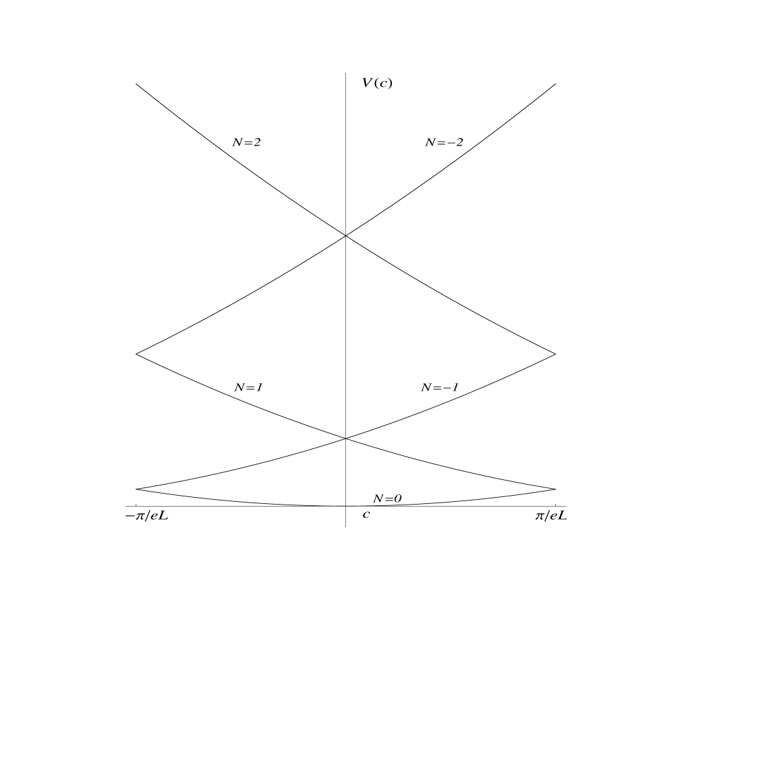
FIG. 1.: The potentials $V_{N}(c)$ in the compact Schwinger model

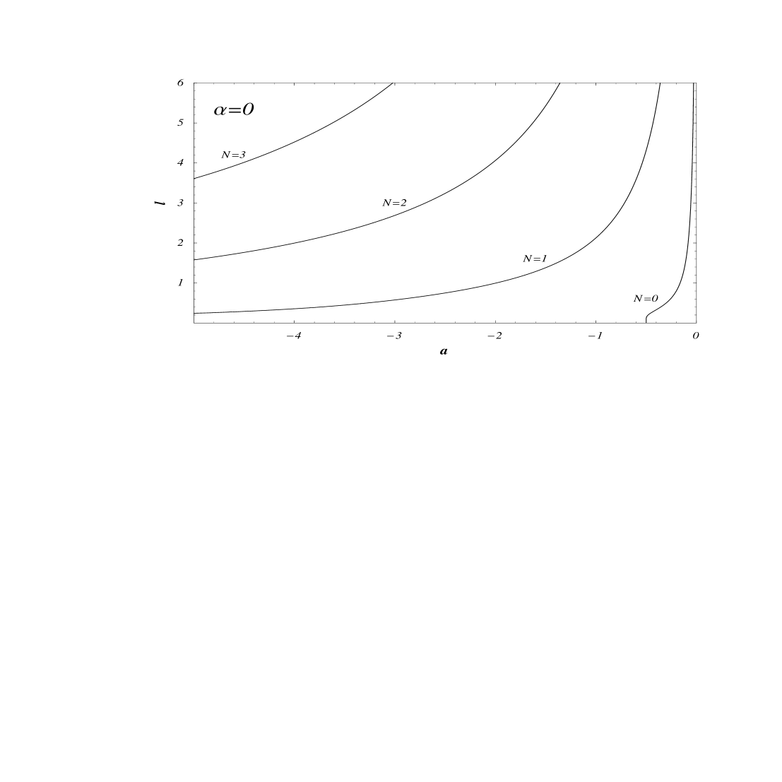
FIG. 2.: The numerical solution for the parameter $a_{0,N}(l)$, for $N=0,1,2,3$ and a given value of $l$. The energies are ${\cal E}_{0,N,0}=-(e/\pi^{1/2})\,a_{0,N}$

FIG. 3.: The numerical solution of $a_{\alpha,N}(l)$, with $N=0,1$ and $\alpha=1,2$, for a given value of $l$, is given. The energies are ${\cal E}_{\alpha,N,0}=-(e/\pi{1/2})\,a_{\alpha,N}$

- [1] J. Schwinger, Phys. Rev. 125, 397 (1962); ibid 128,2425 (1962).
- [2] L.S. Brown, Nuovo Cim. XXIX 3727 (1963); J.H. Lowenstein and J.A. Swieca, Ann. Phys. 68 172 (1971); E. Abdalla and M.C.A. Abdalla, Non-perturbative methods in 2 dimensional quantum field theory (World Scientific, Singapore, 1991).
- [3] For a recent review of the standard Schwinger model see for example C. Adam, Anomaly and Topological aspects of two-dimensional quantum electrodynamics, Dissertation, Universitat Wien, october 1993. See also: C. Adam, CZech J. Phys. 48, 9 (1998); C. Adam, Z. Phys. C63, 169 (1994); C. Adam, R.A. Bertlmann and P. Hofer, Riv. Nuovo Cim. 16, 1 (1993).
- [4] A. Z. Capri and R. Ferrari, Il Nuovo Cimento 62 A, 273(1981).
- [5] N.S. Manton, Ann. Phys. 159, 220 (1985).
- [6] J.E. Hetrick and Y. Hosotani, Phys. Rev. D38, 2621 (1988).
- [7] M.A. Shifman, Phys. Rep. 209, 341 (1991).
- [8] R. Link, Phys. Rev. D42, 2103 (1990).
- [9] S. Iso and H. Murayama, Prog. Theo. Phys. 84,142 (1990).
- [10] J. Hallin and P. Liljenberg, Phys. Rev. D54, 1723 (1996); J. Hallin, QED1+1 by Dirac Quantization, Preprint Göteborg, ITP 93-8, hep-th/9304101, May 1993.
- [11] M. Creutz, Quark, Gluons and Lattices (Cambridge: Cambridge Univ. Press 1983).
- [12] R. Gambini and J. Pullin, Loops, knots, gauge theories and quantum gravity (Cambridge: Gambridge Univ. Press 1996).
- [13] R. Gambini, H. Morales, L. F. Urrutia and J.D. Vergara, Phys. Rev. D57 , 3711 (1998).
- [14] H.Fort and R. Gambini, The U(1) and strong CP problems from the loop formulation perpective, hep-th/9711174, nov. 1997.
- [15] A.M. Polyakov,Gauge Fields and Strings (New York: Harwood 1987).
- [16] M. Asorey, J.G. Esteve and F.A. Pacheco, Phys. Rev. D27,1852(1983).
- [17] R. Linares, L. F. Urrutia and J.D. Vergara in Particles and Fields, Ed. by J. C. D’Olivo, et al, AIP Conference Proceedings 490, (New York, 1999). R. Linares, L. F. Urrutia and J.D. Vergara in JHEP Proceedings, Third Latin American Symposium on High Energy Physics 2000.
- [18] H. Sugawara, Phys. Rev. 170, 1659(1968).
- [19] M. Abramowitz and I. A. Stegun, Handbook of Mathematical Functions (New York: Dover 1965).
- [20] See for example I.S. Gradshteyn and I.M. Ryshik, Table of integrals, Series and Products, Academic Press Inc., New York, 1965, pag. 1074.