SLAC-PUB-8657

SU-ITP 00-25

hep-th/0010105

How Bob Laughlin Tamed the Giant Graviton

from Taub-NUT space

B. A. Bernevig ¹, J. Brodie ², L. Susskind ¹ and N. Toumbas ¹

¹ Department of Physics

Stanford University

Stanford, CA 94305-4060

² Stanford Linear Accelerator Center

Stanford University

Stanford, CA 94309-4349

In this paper we show how two dimensional electron systems can be modeled by strings interacting with $D$-branes. The dualities of string theory allow several descriptions of the system. These include descriptions in terms of solitons in the near horizon $D6$-brane theory, non-commutative gauge theory on a $D2$-brane, the Matrix Theory of $D0$-branes and finally as a giant graviton in M-theory. The soliton can be described as a $D2$-brane with an incompressible fluid of $D0$-branes and charged string-ends moving on it. Including an $NS5$ brane in the system allows for the existence of an edge with the characteristic massless chiral edge states of the Quantum Hall system.

1 Introduction

The dualities of string theory have provided powerful tools for the study of strongly coupled quantum field theories. The most surprising of these dualities involves field theory on one side of the duality and gravitation on the other. For example, Matrix Theory  [1] relates Super Yang Mills theory on various tori to compactifications of 11 dimensional supergravity. Similarly the ADS/CFT duality  [2][3][4][5] relates large $N$ gauge theories to supergravity in an Anti deSitter background. The result is that many problems of quantum field theory such as confinement  [6][7][8][9] and finite temperature  [6][10] behavior are solved by finding classical solutions of the appropriate gravity equations. These solutions include black holes, gravitational waves and naked singularities  [11][12][13].

In view of all these, one may hope that similar correspondences exist involving interesting condensed matter systems. The purpose of this paper is to demonstrate a correspondence between certain solitons in the near horizon geometry of a $D6$-brane and the Quantum Hall System  [14][15] – charged particles moving on a two dimensional surface in the presence of a strong magnetic field. Additional dualities allow a descriptions in terms of $D0$-brane matrix quantum mechanics  [1] and giant gravitons in M-theory.

2 The Brane Setup

We work in uncompactified $IIA$ string theory. Let us begin with a coincident stack of $K$ $D6$-branes whose worldvolume is oriented along the directions $(t,Y^{a})$, where $a=4,...,9$. The three remaining directions we call $X^{i}$, $i=1,2,3$. The $D6$-brane is located at $X^{i}=0$.

Now let us add a spherical $D2$-brane wrapped on the sphere $S_{2}$;

$$\sum_{i=1}^{3}{(X^{i})}^{2}=r^{2}.$$ (2.1)

For the moment let us ignore the stability of this configuration. We would like to show that consistency requires the presence of $K$ fundamental strings connecting the $D6$-branes and the $D2$-brane. To see this, we recall that the $D6$-brane acts as a magnetic source for the Ramond-Ramond gauge field $C_{1}$ which couples electrically to $D0$-branes. In other words the $D6$-brane acts as a magnetic monopole situated at $X^{i}=0$. Let $\tilde{H}_{2}$ denote the $2$-form field strength of $C_{1}$. The flux through the sphere is then given by

$$\int_{S_{2}}\tilde{H}_{2}=2\pi K\mu_{6},$$ (2.2)

where $\mu_{6}$ denotes the elementary $D6$-brane charge. Note also that Dirac’s quantization condition requires that

$$\mu_{6}\mu_{0}=1,$$ (2.3)

where $\mu_{0}$ is the $D0$–brane charge. Evidently, the field strength $\tilde{H}_{2}$ is given by

$$\vec{H}(\vec{r})={K\mu_{6}\hat{r}\over 2r^{2}},$$ (2.4)

where $H_{i}={\epsilon_{i}}^{jk}\tilde{H}_{jk}/2$.

Next recall that $\tilde{H}_{2}$ is coupled to the $D2$-brane world-volume gauge field $A_{\mu}$ through the coupling

$${\mu_{2}\over 2}\int_{S_{2}}\epsilon^{\mu\nu\lambda}(2\pi\alpha^{\prime})A_{\mu}\tilde{H}_{\nu\lambda}=\int_{S_{2}}J^{0}A_{0}$$ (2.5)

with

$$J^{0}={\mu_{2}}(2\pi\alpha^{\prime})|\vec{H}(\vec{r})|={\mu_{2}\mu_{6}K(2\pi\alpha^{\prime})\over 2r^{2}}.$$ (2.6)

The expression above corresponds to a background charge density on the $D2$-brane with total charge

$$Q=2\pi K\mu_{2}\mu_{6}(2\pi\alpha^{\prime}).$$ (2.7)

Since branes are BPS objects the ratio of their charges is equal to the ratio of their tensions. Thus $\mu_{2}=\mu_{0}(T_{2}/T_{0})$. Then using eq. (2.3), we obtain

$$Q=2\pi K(2\pi\alpha^{\prime}){T_{2}\over T_{0}}=K.$$ (2.8)

This background charge must be cancelled since the total charge on a compact space must vanish. Thus we must add $K$ strings stretched between the $D6$ and the $D2$ branes.

This result is closely related to the Hanany-Witten effect  [16]. Begin with the $D2$-brane far from the $D6$-branes and not surrounding them. Now move the membrane towards the six branes. As the $D6$-branes pass through the $D2$-brane, the Hanany-Witten effect adheres the strings. Later we will give a Matrix Theory argument for the same result.

Figure 1: Stable spherical D2-brane with $N$ units of magnetic flux surrounding K D6-branes. K fundamental strings stretch from the D2-brane to the D6-brane. There is a uniform density of negative charge on the sphere due to the field generated by the D6-brane.

3 Balancing The System

The system as described is not stable. The tension of the $D2$-brane and the $K$ strings will cause the spherical $D2$-brane to collapse. To counteract this let us add $N$ $D0$-branes dissolved in the $D2$-brane. It is well known that $D6$-branes and $D0$-branes repel one another. The dissolved $D0$-branes give rise to a magnetic flux on the $D2$-brane world volume. The integrated flux is just the $N$ units of $D0$-brane charge. As we will see the repulsion can stabilize the radius of the $D2$-brane. The resulting object we will call a Quantum Hall Soliton.

We will work in the approximation that the $D2-D0$ system is a test probe in the $D6$-brane geometry. In other words we ignore the backreaction of the $D2-D0$ system on the geometry. The backreaction will alter the precise details but we do not expect it to change the scalings that we find.

The string frame metric of the $K$ $D6$-branes is given by

$$ds_{6}^{2}=h(r)^{-{1\over 2}}dt^{2}-h(r)^{-{1\over 2}}dy^{a}dy^{a}-h(r)^{1\over 2}dr^{2}-h(r)^{1\over 2}r^{2}d\Omega_{2}^{2}$$ (3.1)

with $h(r)$ given by

$$h(r)=1+{Kg_{s}l_{s}\over 2r},$$ (3.2)

where $g_{s}$ and $l_{s}$ are the string coupling constant and length scale. The background dilaton field is given by

$$g_{s}^{2}e^{2\Phi}=g_{s}^{2}h(r)^{-{3\over 2}}.$$ (3.3)

We will choose parameters so that the $D2$-brane is well within the near horizon region in which we can set

$$h(r)={Kg_{s}l_{s}\over 2r}.$$ (3.4)

It will be convenient to rescale the co-ordinates

$$\tilde{y}=\left({Kg_{s}\over 2}\right)^{1\over 3}y,\,\ t=\left({Kg_{s}\over 2}\right)^{1\over 3}\tau,\,\ r=\left({Kg_{s}\over 2}\right)^{-{1\over 3}}\rho$$ (3.5)

so that the metric becomes

$$ds^{2}=\sqrt{\rho\over l_{s}}(d\tau^{2}-d\tilde{y}^{a}d\tilde{y}^{a})-\sqrt{l_{s}\over\rho}(d\rho^{2}+\rho^{2}d\Omega_{2}^{2}).$$ (3.6)

The background dilaton becomes then

$$g_{s}^{2}e^{2\Phi}={4\over K^{2}}\left({\rho\over l_{s}}\right)^{3\over 2}.$$ (3.7)

Now consider the $D2$–brane wrapped on the $2$-sphere with $N$ units of $D0$-brane charge or equivalently, $N$ units of magnetic flux. As in the previous section, we must add $K$ $6-2$ strings which we orient along the radial direction. The action for the $D2$–brane in the background geometry is given as usual by the Dirac Born Infeld (DBI) action. From the DBI action of the brane plus the action of the strings we can obtain a potential for the radial mode $\rho$.

We choose worldvolume co–ordinates such that

$$\xi^{0}=\tau,\,\ \xi^{1}=\theta,\,\ \xi^{2}=\phi.$$ (3.8)

Dropping time derivatives, the induced metric on the brane $G_{ab}$ becomes

$$G_{00}=\sqrt{\rho\over l_{s}},\,\ G_{11}=-\sqrt{\rho^{3}l_{s}},\,\ G_{22}=-\sqrt{\rho^{3}l_{s}}\sin^{2}\theta.$$ (3.9)

In addition, there are $N$ units of flux on the brane:

$$\int_{S_{2}}F=2\pi N.$$ (3.10)

Thus the background field on the brane is given by

$$F_{12}={N\over 2}\sin\theta.$$ (3.11)

This corresponds to a constant field strength perpendicular to the 2-sphere.

The DBI Lagrangian for the brane is then given by

$$L_{D2}=-{1\over 4\pi^{2}g_{s}l_{s}^{3}}\int d\theta d\phi e^{-\Phi}det[G_{ab}+2\pi l_{s}^{2}F_{ab}]^{1\over 2}=-{K\rho\over 2\pi l_{s}^{2}}\sqrt{1+{\pi^{2}N^{2}l_{s}^{3}\over\rho^{3}}}.$$ (3.12)

The contribution of the $K$ strings is given by

$$L_{Strings}=-{K\over 2\pi l_{s}^{2}}\rho.$$ (3.13)

Therefore, the potential for $\rho$ becomes

$$V(\rho)={K\rho\over 2\pi l_{s}^{2}}\left(\sqrt{1+{\pi^{2}N^{2}l_{s}^{3}\over\rho^{3}}}+1\right).$$ (3.14)

The potential has a minimum at

$$\rho_{*}={({\pi N})^{2\over 3}\over 2}l_{s}$$ (3.15)

for all $N$ and $K$. Thus the brane can stabilize at this co–ordinate distance.

We require that our brane lives in the near horizon region. Therefore, we must have

$$h(\rho_{*})>1$$ (3.16)

or that

$$g_{s}>{\sqrt{N}\over K}$$ (3.17)

at infinity. For fixed $K/N$ and any value of $g_{s}$ this will be satisfied for large enough $N$.

The proper area of the stable membrane is given by

$$A=4\pi\sqrt{{\rho_{*}}^{3}l_{s}}=\sqrt{2}\pi^{2}Nl_{s}^{2}.$$ (3.18)

The fact that the $D0$-brane density is universal in string units is noteworthy. It means that the $D0$-brane system is behaving like an incompressible fluid. This also implies that the magnetic field and the magnetic length is fixed.

Let us next consider the gauge coupling of the theory on the $D2$-brane. The theory is an abelian gauge theory with coupling constant given by

$$g_{YM}^{2}l_{s}=g_{s}e^{\Phi}|_{\rho_{*}}={2\over K}\left({\rho_{*}\over l_{s}}\right)^{3\over 4}=2^{1\over 4}{\sqrt{\pi N}\over K}$$ (3.19)

independent of $g_{s}$ at infinity.

In the Quantum Hall interpretation of the system $K$ plays the role of the number of charged particles and $N$ the total magnetic flux. The ratio $K/N=\nu$ is the filling fraction which we will want to keep fixed as $N\rightarrow\infty$. We therefore find

$$g_{YM}^{2}\sim{1\over\nu\sqrt{N}l_{s}}.$$ (3.20)

We also note that the curvature of the background geometry at $\rho_{*}$ is given by

$$l_{s}^{2}{\cal{R}}\sim{1\over N}$$ (3.21)

and so it is weak for large $N$. Thus we can reliably use the DBI action to study the dynamics of the system. Finally, the $D0$–brane magnetic field through the sphere is fixed in string units $|\vec{H}|\sim\mu_{6}K/Nl_{s}^{2}\sim\mu_{6}\nu/l_{s}^{2}$.

4 Energy Scales

In this section we will see that a single energy scale controls the dynamics of the Quantum Hall Soliton. In discussing these energy scales we will work in units appropriate to a local observer at the $D2$-brane. In other words, let us once again rescale time so that proper time at the $D2$-brane is $T$:

$$dT^{2}=\sqrt{\rho_{*}\over l_{s}}d\tau^{2}$$ (4.1)

or

$$dT={({\pi N})^{1\over 6}\over 2^{1\over 4}}d\tau.$$ (4.2)

The energy scales we derive refer to the Hamiltonian conjugate to $T$.

Quasiparticle Coulomb Energy. Quantum hall fluids are said to be incompressible. By this it is meant that the system has an energy gap, namely the energy of a quasiparticle. Later we will discuss the formation of fractionally charged quasiparticles [14]. For the moment, we can just regard a quasiparticle as a localized object with charge $\pm\nu$ and a radius of order the magnetic length. It has a Coulomb energy of order

$$E_{Quas}\sim(g_{YM}\nu)^{2},$$ (4.3)

which from eq. (3.20) is

$$E_{Quas}\sim{\nu\over\sqrt{N}l_{s}}.$$ (4.4)

This is the basic energy scale of quantum hall excitations against which other energies should be compared.

Long String Excitations. If a string of length $L$ is vibrationally excited, its energy is of order $1/L$. The proper length of the $6-2$ strings is of order

$$L\sim{({\rho_{*}}^{3}l_{s})}^{1\over 4}$$ (4.5)

and so using eq. (3.16) we find

$$L\sim\sqrt{N}l_{s}$$ (4.6)

corresponding to an energy scale

$$E_{String}\sim{1\over\sqrt{N}l_{s}}.$$ (4.7)

Note that this scales with $N$ in the same way as the quasiparticle energy but it is typically bigger by a factor $1/\nu$.

Cyclotron Frequency. The energy required to excite a higher Landau level is given by the cyclotron frequency

$$\omega_{Cycl}={B\over m},$$ (4.8)

where $B$ is the magnetic field and $m$ is the mass of a charge. The charges are strings of mass $L/l_{s}^{2}$ and in string units $B\sim 1$. Therefore,

$$\omega_{Cycl}\sim{1\over\sqrt{N}l_{s}}.$$ (4.9)

Once again this scales like the quasiparticle energy but it is bigger by the factor $1/\nu$.

Field Theory Gap. Since the radius of the 2-sphere is $\sim N^{1/2}l_{s}$ the energy of the lowest field mode living on the $D2$-brane is of order $1/N^{1/2}l_{s}$. Later we will see that the gauge field has a mass of the same order of magnitude.

As we have seen the radius of the $2$-sphere is stabilized by the competing terms in the DBI potential. The spherically symmetric fluctuations about this equilibrium are described by a massive scalar field. By expanding the DBI action to quadratic order in the fluctuations, we find the mass to again be $\sim 1/N^{1/2}l_{s}$. Thus we see a single energy scale governing all of low energy physics on the membrane.

Again it is noteworthy that a single energy scale appears in the low energy behavior. By an additional rescaling of time (which we will not do) the energy and time scales for the system can all be made to be of order unity. Unless $\nu\ll 1$, there is no large separation of energy scales. Our assumption will be that despite the lack of large scale separation the quantum hall effect is robust, at least for $\nu$ not too large.

4.1 $D0$-Brane Emission

For finite $N,K$ the Quantum Hall Soliton  can not be absolutely stable. The $D2$-brane carries no net charge. If the $D0$-branes escape from the membrane they will be repelled to infinity, leaving the $D2$-brane to collapse and disappear. We will argue that the emission of a $D0$-brane is a tunneling process with a barrier that becomes infinite as $N,K$ become large.

The value of the potential (3.14) at the minimum $\rho_{*}$ is given by

$$V(\rho_{*})={KN^{2\over 3}\over\pi^{1\over 3}l_{s}}.$$ (4.10)

This corresponds to a proper $T$-energy given by

$$V_{T}(\rho_{*})={2^{1\over 4}K\sqrt{N}\over\sqrt{\pi}l_{s}}.$$ (4.11)

Suppose that the system emits a $D0$-brane so that the flux changes by one unit. Then to leading order in $1/N$ the change in the energy is given by

$$V_{T}(N)-V_{T}(N-1)={K\over 2^{3\over 4}\sqrt{\pi N}l_{s}}.$$ (4.12)

This is of the same order of magnitude as the mass of a $D0$-brane just outside the brane but smaller by a factor of $\sqrt{2}$:

$$M_{D0}={1\over g_{s}(\rho_{*})l_{s}}={K\over 2^{1\over 4}\sqrt{\pi N}l_{s}}.$$ (4.13)

Therefore, we can estimate the binding energy of a $D0$-brane to be of order

$$E_{bind}\sim{\nu N^{1\over 2}\over l_{s}}.$$ (4.14)

This binding energy represents the height of the tunneling barrier and it becomes infinite with $N$. It is not hard to see that the width of the barrier also becomes infinite. Thus the process of $D0$-brane emission is very suppressed in the large $N$ limit.

There is another possible mode of instability that was pointed out to us by Maldacena  [26]. It is possible for the $D6$-brane to nucleate a second spherical $D2$-brane at a small radius. In this configuration the strings from the original outer 2-sphere terminate on the concentric inner 2-sphere. If the system lowers its energy when the inner sphere expands, it will be unstable, the inner and outer spheres annihilating one another.

The potential for the inner sphere can be obtained from that of the outer sphere, eq. (3.14) by making two changes. First of all, since the $D0$-brane charge on the inner sphere vanishes $N$ should be set to zero. Secondly since the strings are now on the outside of the $2$-sphere the sign of the last term in (3.14) should be changed. The result is a vanishing potential which indicates that the inner brane is in neutral equilibrium. Thus there is no tendency for the inner brane to expand, at least within the context of our approximations.

Klebanov  [26] has pointed out a way to stabilize the inner brane at vanishing radius. If we retain the full form of the harmonic function $h$ in eq. (3.2) the perturbation due to the first term leads to a correction which makes the potential minimum when the inner brane vanishes.

The stability of the Quantum Hall Soliton with respect to non-spherically symmetric perturbations has not yet been carried out.

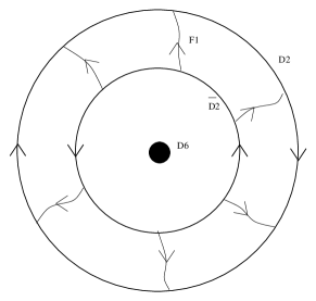
Figure 2: Two D2-branes surround a D6-brane. The two D2-branes have opposite orientation. There are $N$ units of flux on the outer D2-brane. $K$ strings now stretch between the two D2-branes.

5 The Membrane Theory

In this section we work in some detail the theory describing the fluctuations of the membrane. The proper size of the sphere grows like $N^{1/2}$ in string units. Thus we can focus on a patch much larger than the magnetic length and approximate it as flat. We choose co–ordinates such that the metric is the standard flat metric. The cartesian coordinates in the $D2$-brane will be called $x^{i}$, $i=1,2$.

Without the $D0$-branes and at low energies, the theory describing the fluctuations of the $D2$-brane is expected to be a $U(1)$ abelian gauge theory. Now let us dissolve the $N$ $D0$–branes. Dissolving the $D0$–branes essentially turns the membrane into a non–commutative membrane. In general, the low energy dynamics of the theory is expected to be governed by a $U(1)$ non–commutative Yang Mills theory. However, this is not the end of the story. As we have seen in eq. (2.4) the presence of the $D6$–branes induces a $D0$–brane magnetic field ( not to be confused with the world volume magnetic field $B$ on the $D2$-brane ). Thus a single $D0$-brane in this field will experience a Lorentz force governed by a term in its Lagrangian

$$L={\mu_{0}H_{3}\over 2}\epsilon_{ij}X^{i}D_{t}X^{j},$$ (5.1)

where $i,j=1,2$ and

$$D_{t}X=\dot{X}-i[A_{0},X].$$ (5.2)

For studying the many $D0$-brane  system we use Matrix Theory  [1]. The Matrix Theory action corresponding to eq. (5.1) is

$$L={\mu_{0}H_{3}\over 2}\epsilon_{ij}TrX^{i}D_{t}X^{j},$$ (5.3)

where $i,j=1,2$. This Lagrangian is invariant under the infinitesimal gauge transformations

$$X\rightarrow X+i[\lambda(t),X].$$ (5.4)

Indices are raised and lowered by the ‘closed string’ metric $g_{\mu\nu}$ which we choose to be the standard one.

The effect of this term is two-fold. It first of all induces a background charge density as in eq. (2.8). In addition it produces a Chern Simons coupling  [15]. To find the new couplings we construct a large membrane from $N$ $D0$ branes moving in a constant background $H$–field, $H_{3}=2\pi\mu_{6}/V$, where $V$ is the volume of the membrane.

Following [17], we choose matrices $x^{1}$ and $x^{2}$ such that

$$[x^{i},x^{j}]=i\theta\epsilon^{ij}$$ (5.5)

and set

$$X^{i}=x^{i}+\theta\epsilon^{ij}A_{j}(x^{i}).$$ (5.6)

The $x^{i}$’s are constant matrices to be identified with the non–commuting co-ordinates of the membrane. Such matrices exist strictly for infinite $N$ and are classical solutions to the equations of motion. The $A_{j}$’s are fluctuations around the classical solutions $X^{i}_{clas}=x^{i}$ and these will map to the gauge field living on the brane. Any matrix can be expressed in terms of finite sums of products $e^{ipx^{1}}e^{iqx^{2}}$; so the $N\times N$ matrices $A_{i}$ can be thought of as functions of the $x^{i}$’s.

We now insert eq. (5.6) in (5.3) to find an effective Lagrangian for the fluctuations $A_{i}$. Dropping total time derivatives we end up with

$$L_{eff}={\pi K\over V}\left(i\epsilon_{ij}Tr[x^{i},x^{j}]A_{0}-\theta^{2}\epsilon^{ij}TrA_{i}\partial_{t}A_{j}+2i\theta\epsilon_{ij}Tr[x^{i},\epsilon^{jk}A_{k}]A_{0}+2i\theta^{2}\epsilon^{ij}Tr[A_{i},A_{j}]A_{0}\right).$$ (5.7)

Using eq. (5.5) and

$$[x^{i},f]=i\theta\epsilon^{ij}\partial_{j}f,$$ (5.8)

we can simplify this as follows

$$L_{eff}={\pi K\over V}\left(-2\theta TrA_{0}-\theta^{2}\epsilon^{ij}TrA_{i}\partial_{t}A_{j}+\theta^{2}\epsilon^{ij}Tr\partial_{i}A_{j}A_{0}-\theta^{2}\epsilon^{ij}Tr\partial_{i}A_{0}A_{j}+2i\theta^{2}\epsilon^{ij}Tr[A_{i},A_{j}]A_{0}\right).$$ (5.9)

Finally, introducing the totally antisymmetric tensor $\epsilon^{\mu\nu\rho}$, we can write this as

$$L_{eff}=-{2\pi K\over V}\theta TrA_{0}+{\pi K\over V}\theta^{2}\epsilon^{\mu\nu\rho}\left(TrA_{\mu}\partial_{\nu}A_{\rho}+{2\over 3}iTrA_{\mu}A_{\nu}A_{\rho}\right).$$ (5.10)

Now we pass to the continuum limit taking $N$ large. We identify as usual

$$\theta Tr\leftrightarrow\int{dx^{1}dx^{2}\over 2\pi}.$$ (5.11)

This requires that

$$\theta={V\over 2\pi N}.$$ (5.12)

We see that $\theta$ is nothing more than the inverse magnetic field $B$ through the brane. The magnetic length sets the scale of non–commutativity  [18][19].

The $N\times N$ matrices $A_{i}$ will map to smooth functions $A_{i}(x^{i})$ of the non–commutative co–ordinates $x^{i}$. Since the fields are functions of non–commuting co–ordinates, we need to define a suitable ordering for their products in the Lagrangian. A suitable ordering is Weyl ordering which means that ordinary products are replaced by the non–commutative $*$ product. In all, we end up with the following action

$$S_{eff}=\int d^{3}xA_{0}J^{0}+{K\over 4\pi N}\epsilon^{\mu\nu\rho}\left(A_{\mu}*\partial_{\nu}A_{\rho}+{2\over 3}iA_{\mu}*A_{\nu}*A_{\rho}\right).$$ (5.13)

Here, $J^{0}=-K/V$ and so there is a net background charge $-K$ on the brane. To cancel this background charge we add $K$ string ends on the brane. The action is a $U(1)$ NC CS action at level $K/4\pi N$ and non–commutativity parameter $\theta=V/2\pi N$ plus the chemical potential term $A_{0}J^{0}$.

In addition to the terms induced by $H$ there is a $U(1)$ NC Maxwell term. This term has been constructed in [17]. It is given by

$${1\over 2g_{YM}^{2}}\int d^{3}x(detG_{\mu\nu})^{1\over 2}G^{\mu\rho}G^{\nu\sigma}\ (F+\Phi)_{\mu\nu}*(F+\Phi)_{\mu\nu}$$ (5.14)

where $F_{\mu\nu}=\partial_{\mu}A_{\nu}-\partial_{\nu}A_{\mu}+[A_{\mu},A_{\nu}]_{*}$ and $\Phi_{\mu\nu}=-\theta^{-1}_{\mu\nu}$. The indices are contracted with the effective metric $G_{\mu\nu}$

$$G_{00}=1,\,\ G_{11}=G_{22}=-(2\pi\alpha^{\prime})^{2}\theta^{-2},$$ (5.15)

and the coupling constant is given by

$$g_{YM}^{2}\sim{g_{s}(\rho_{*})(2\pi\alpha^{\prime}\theta^{-1})\over l_{s}}.$$ (5.16)

The dimensionless string coupling constant $g_{s}(\rho_{*})$ is of course a function of the distance from the $6$–branes. As we found in eq. (3.19) $g_{s}(\rho_{*})\sim 1/\nu\sqrt{N}$.

As noted by Seiberg [17] the action in eq. (5.14) is of the usual non–commutative type except for the shift of the field strength by amount $\Phi$. This shift is of course due to the presence of a background magnetic field. The Lagrangian differs by the standard minimal Lagrangian, $F^{2}$, by a constant term and a total derivative. Although this makes no change in the equation of motion, it does have the effect from shifting the value of $F$ from zero to $-\Phi=\theta^{-1}$ in the ground state.

As we found in eq. (3.18) the volume of the membrane (measured in closed string units) scales like

$$V\sim N\alpha^{\prime}.$$ (5.17)

Then

$$\theta\sim\alpha^{\prime},$$ (5.18)

and the separation of the constituent $D0$–branes is fixed in string units. The effective metric is then

$$G_{00}=1,\,\ G_{ij}\sim(-1,-1)$$ (5.19)

and the Maxwell coupling constant is given by

$$g_{YM}^{2}\sim{g_{s}(\rho_{*})\over l_{s}}\sim{1\over\nu\sqrt{N}l_{s}}.$$ (5.20)

Although the Chern-Simons term is interesting, it has nothing to do with the usual Chern-Simons description of the Quantum Hall fluid of electrons. This electron fluid may also be described by a CS theory  [15]. This suggests that the coupled system of sting ends and $D0$-branes may be described by two coupled CS theories, one describing the electron fluid and the other the fluid of $D0$-branes.

The CS term in eq. (5.13) does not influence the physics at scales much smaller than the size of the entire 2-sphere. This is because the gauge coupling is very weak. For example the gauge boson mass induced by the Chern Simons term is

$$m_{ph}\sim 2g_{YM}^{2}\nu\sim{1\over\sqrt{N}l_{s}}.$$ (5.21)

In other words the Compton wavelength of the photon is of order the sphere radius. At somewhat shorter distances the forces are dominated by the ordinary $2+1$ dimensional Coulomb repulsion. At distances smaller than the string scale the forces are softened by the effects of non–commutativity and other stringy effects. The fact that the Compton wavelength of the photon is so large means that there is no meaningful effect on the statistics of the charges, at least when they are separated by distances smaller than the size of the sphere. For larger distances the Chern-Simons term may introduce phases but this should not affect the local physics on smaller scales.

Thus far we have discussed the gauge field on the $D2$-brane. There are additional world volume fields such as scalars and spinors which all have similar mass and are described by the appropriate non–commutative fields. However the list of degrees of freedom would not be complete without the all important electrons. From the point of view of the $D2$-brane Matrix Theory, these are not described by matrices but rather column vectors (or the conjugate row vectors). Such fields form fundamental representations of the non–commutative gauge invariance and we describe them by either fermionic or bosonic fields $|\Psi\rangle$ and $\langle\Psi^{{\dagger}}|$. The appropriate gauge invariant action for these fields is very simple:

$$L_{\Psi}=\langle\Psi^{{\dagger}}|(i\partial_{t}+A_{0})|\Psi\rangle+\langle\Psi^{{\dagger}}|m|\Psi\rangle.$$ (5.22)

The full action is obtained by adding eq. (5.10) to $L_{\Psi}$

$$S_{eff}=-{K\over N}TrA_{0}+\langle\Psi^{{\dagger}}|(i\partial_{t}+A_{0})|\Psi\rangle+\langle\Psi^{{\dagger}}|m|\Psi\rangle+....$$ (5.23)

Varying this action with respect to $A_{0}$ and taking the trace we find that the total number of electrons is $K$

$$\langle\Psi^{{\dagger}}|\Psi\rangle=K.$$ (5.24)

6 D6-Brane Dynamics

The near horizon physics of the $D6$-brane system is described by a $6+1$-dimensional theory which at long distances is a supersymmetric gauge theory. Indeed the configuration we are studying may be thought of as a soliton of the $D6$-brane theory. The only charge carried by the soliton is the $D0$-brane charge $N$. The spherical $D2$-brane carries no net charge. To interpret the charge $N$ in the $SU(K)$ gauge theory, we recall that there is a coupling between the $D6$-brane worldvolume gauge field $F$ and the bulk field $C_{1}$

$$\int_{7}C_{1}\wedge F\wedge F\wedge F.$$ (6.1)

Since $C$ is sourced by the $D0$-brane charge, it follows that our configuration satisfies

$$\int_{6}F\wedge F\wedge F\sim N.$$ (6.2)

Such a classical gauge configuration is unstable with respect to collapse; that is, it wants to collapse to zero size. Evidently, this behavior is resolved in the quantum theory by the $D2$-brane system. Although the soliton is not absolutely stable, in the limit $N,K\rightarrow\infty$, the tunneling barrier for the emission of a $D0$-brane from the $D2$-brane becomes infinite.

Let us consider the strength of the $SU(K)$ couplings on the $D6$-brane system. The gauge coupling is given by

$$g_{6}^{2}=g_{s}(\rho).$$ (6.3)

In this formula, $g_{6}^{2}$ refers to the dimensionless coupling at the proper length scale $l_{s}$. Next we use

$$g_{s}(\rho)={2\over K}{\left({\rho\over l_{s}}\right)}^{3\over 4}.$$ (6.4)

The ‘t Hooft coupling is given by

$$Kg_{s}(\rho)\sim{\left({\rho\over l_{s}}\right)}^{3\over 4}.$$ (6.5)

This equation makes it appear that the coupling vanishes as we approach $\rho=0$. However, the gauge coupling has dimensions of length to the cubic power. To determine the effective dimensionless coupling at a co-ordinate length scale $\Delta\tilde{y}$, we should divide by three powers of the corresponding proper length. From the metric, eq. (3.6), we see that the proper length is given by

$${\left(\rho\over l_{s}\right)}^{1\over 4}\Delta\tilde{y}.$$ (6.6)

We need, therefore, to divide by $(\rho/l_{s})^{3/4}{\Delta\tilde{y}}^{3}$. so that the strength of the dimensionless coupling at a co-ordinate scale $\Delta\tilde{y}$ is given by

$${\left(l_{s}^{3}\over\Delta\tilde{y}\right)}^{3}.$$ (6.7)

Thus at $\Delta\tilde{y}$ of order one in string units, the $D6$-brane theory becomes strongly coupled.

Now consider the $K$ string ends on the $D6$-brane. These objects are analogous to non-relativistic quarks in QCD. Their gauge interactions become strong at separations $\Delta\tilde{y}\sim l_{s}$. Let us assume that they bind into an $SU(K)$ singlet, “baryon,” of this size. We would like to compare the energy scales of the baryon-excitations with the energy scales discussed in section (4). In this discussion, energy means conjugate to $\tau$.

The excitation energy of the baryon is of order one in string units since the natural scale is $\Delta\tilde{y}\sim l_{s}$. As we saw in section (4), the proper energy ($T$-energy) of string oscillations, higher Landau levels and quasiparticles is of order $N^{-1/2}$ in string units. To convert this to $\tau$-energy, we need to multiply by a factor ${g_{00}}^{1/2}$ at the $D2$-brane. For example, the quasiparticle $\tau$-energy is given by

$$E_{Quas}\sim{{\rho_{*}}^{1\over 4}\over\sqrt{N}}\sim N^{-{1\over 3}}.$$ (6.8)

The implication is that the energy scale of the baryon-excitations is much larger than the excitation scales of the $D2$-brane. In the sense of the Born-Oppenheimer method, the baryon degrees of freedom are fast degrees of freedom.

7 Properties of the Electron System

The string-ends that move on the $D2$-brane are charged particles with respect to the membrane world-volume gauge theory. We will refer to them as electrons. In this section we discuss their properties.

7.1 The Statistics of the Charges

As we will see, the question of the statistics of the electron string-ends on the $D2$-brane is far from straightforward.

Consider a ground string state connecting the $D6$ and $D2$ branes. General string theory arguments given in the appendix tell us that these strings satisfy fermionic statistics. However, the fact that the full $6-2$ strings are fermions, does not imply that the electrons on the $D2$-brane are fermions. A simplified model illustrates the subtleties. We will assume that the $6-2$ strings remain in their ground state apart from the motion of their end-points on the branes. In our approximation, the motion of each of the two string ends is independent of the motion of the other. Then a string is characterized by a location on the $D2$-brane $x$ and a location on the $D6$-branes $y$. In addition, it has an $SU(K)$ index $i$ labeling which $D6$-brane it ends on. As we saw, the strings are fermions. The $K$-body wavefunction has to be antisymmetric with respect to simultaneous interchange of any pair of labels $(x,y,i)$.

Concerning the $SU(K)$ indices we assume that they combine to form a singlet. In the previous section, we discussed the gauge interactions on the $D6$-brane. Although, the string coupling vanishes at the $D6$-brane, the ‘t Hooft coupling is large at length scales $\Delta\tilde{y}\sim l_{s}$. Therefore, we expect that any non-singlet configuration would radiate gauge bosons until it discharged. Since the singlet wavefunction is antisymmetric with respect to the $SU(K)$ indices, the remaining wavefunction must be symmetric.

The most naive assumption about the behavior of the ends on the $D6$-brane is that they are all localized at $y=0$. This would mean that the wavefunction is symmetric with respect to interchange of the $y$ coordinates. In this case the electrons are bosons since the dependence on the $x$ coordinates is also symmetric.

The reason that this may be naive is that the gauge forces on the $D6$-brane between string ends may not be weak if they are localized with small separation. In other words the dynamics of the “knot” where all the strings come together may be non-trivial. Perhaps it is possible that an antisymmetric sector for the baryon wavefunction exists.

We will consider two possible sectors of the theory. In the first sector the wavefunction of the $y$ co-ordinates is symmetric and the electrons are bosons while in the second sector it is antisymmetric and the electrons are fermions. We do not know which sector has the lower energy but as far as the fast dynamics of the $D6$-brane interactions is concerned, the two sectors are uncoupled superselection sectors. Thus the $K$-body wavefunction of the strings can have either one of the following forms

$$\Psi_{1}=\phi_{s}(x_{1},...,x_{k})\epsilon_{i_{1}i_{2}..i_{k}}{\psi_{s}}^{i_{1}i_{2}..i_{k}}(y_{1},...,y_{k}),$$ (7.1)

and

$$\Psi_{2}=\phi_{a}(x_{1},...,x_{k})\epsilon_{i_{1}i_{2}..i_{k}}{\psi_{a}}^{i_{1}i_{2}..i_{k}}(y_{1},...,y_{k}),$$ (7.2)

where $\phi_{s},\psi_{s}$ and $\phi_{a},\psi_{a}$ are symmetric and antisymmetric functions of their arguments respectively.

Our primary interest in this paper is in the physics described by the wavefunctions $\phi(x)$. These wavefunctions describe the physics of $K$ charged fermions, if $\phi$ is antisymmetric, or $K$ charged bosons if $\phi$ is symmetric. The particles move on a $2$-sphere with $N$ units of magnetic flux. Thus the low lying spectrum of states should be that of the bosonic or fermionic Quantum Hall system with filling fraction

$$\nu={K\over N}.$$ (7.3)

Without further evidence we will assume that the conventional Quantum Hall phenomenology applies to our system. For example, we assume incompressible Quantum Hall states exist for all odd denominator $\nu$’s in the fermion case and even denominator $\nu$’s in the bosonic case.

7.2 Quasiparticles

An important feature of the Quantum Hall effect is the existence of an energy gap and fractionally charged quasiparticles. Let us briefly review the construction of these objects  [20][21].

First begin with the theory on the plane. The lowest Landau level (LLL) wavefunctions are degenerate and there is one orthogonal LLL for each unit of magnetic flux. It is helpful to make an identification of the LLL’s with the flux quanta. In the stringy construction in this paper, the flux quanta are the $D0$-branes. Each $D0$-brane can be thought of as a LLL and a string ending on that $D0$-brane is an electron in that LLL. Since the $N$ LLL’s are degenerate, there is a $U(N)$ symmetry of the space of LLL’s. This $U(N)$ symmetry is just the $U(N)$ gauge invariance of the Matrix Theory description of $D0$-branes. It is also a regularized version of the area preserving diffeomorphism group.

The conventional construction of a quasiparticle begins with the idea of an infinitely thin solenoid passing through the substrate [20]. The magnetic field through the substrate is adiabadically increased until the flux equals one Dirac unit. The new gauge field is a gauge transformation of the old, but the process induces a change in the state of the system. To understand the change, it is convenient to work in a basis of angular momentum LLL’s, $|l>$. The individual angular momentum wavefunctions are concentrated on circular rings of radius $\sim l^{1/2}$ with the solenoid at the center. Turning on the solenoid-flux, takes each electron in the $l$-th state to the $l+1$ state but in the process the $l=0$ state is left unoccupied. The result is a hole in the electron density. Since each LLL had originally an average charge $\nu=K/N$, the hole has charge $\nu$. The radius of the hole is just the magnetic length and it is independent of the charge.

Another way to construct the quasiparticle is to begin with a distant magnetic monopole one one side of the substrate. Adiabadically passing the magnetic monopole through the substrate to the other side has the same effect as turning up the current in the solenoid. The monopole picture is especially relevant for the spherical substrate. Transporting the monopole from outside to inside the sphere creates an additional unit of magnetic flux but does not increase the number of electrons. The result is a hole at the place where the monopole passed through the sphere.

An intuitive way to think about these effects is to picture the magnetic flux as an incompressible fluid with the electrons moving with the fluid. When a new unit of flux is added it pushes the fluid away, creating a hole in the electron density. As we have seen the $D0$-brane fluid does in fact behave incompressibly.

In the string/brane setup of this paper, there are neither solenoids nor monopoles. In fact, the $2$-sphere does not divide space into an inside and outside. A possibility that comes to mind is to pass a $D6$-brane through the $2$-sphere but this has the effect of changing the electron number by one unit, not the flux.

The key to the formation of the quasiparticle is the $D0$-brane. We have previously seen that the dissolved $D0$-branes form an incompressible fluid. We introduce an additional $D0$-brane far away from the substrate $2$-sphere. Now adiabadically allow it to approach the $2$-sphere at some point $x_{0}$. At some distance of order $l_{s}$, it will get absorbed by the $D2$-brane adding a unit of flux at $x_{0}$ to the original $N$ units. The flux behaving like an incompressible fluid will increase the area of the sphere by one unit, leaving a hole of charge $\nu$ in the charged particle distribution at the point $x_{0}$.

The quasi particle defined in this way is not necessarily stable. As an example consider the fermionic case $\nu={p/(2p+1)}$ with integer $p$. Now take two quasiparticles of charge $\nu$ and combine them with one extra electron. If they bind, the result is a new quasiparticle of charge $-1/(2p+1)$. (It is also possible to create an excitation with charge $+1/(2p+1)$). In this case the original quasiparticle can decay into $p$ constituents. The quasiparticle with charge $-1/(2p+1)$ can be constructed by starting with an extra $6-2$ string with two $D0$-branes attached to it. By sliding the $D0$-branes toward the membrane until they dissolve, the new quasiparticle is created. In the limit $p\to\infty$ the neutral quasiparticle of the $\nu=1/2$ state results [22].

Figure 3: The figure shows two D0-branes on a fundamental string. The string ends on a D2-brane.

7.3 Composite Fermions

The qualitative features of the QHE have been nicely captured by a phenomenological model, the so called composite fermion model (CFM)  [23]. While the theoretical underpinnings of the CFM are not completely secure, it does appear to successfully correlate many properties of the various fractional QHE ground states.

We make no claim in this paper to deriving the CFM. However we do think the language of string theory is suggestive and might offer new insights. We regard it as a challenge to use the tools of string theory and non–commutative field theory to give a derivation. What we will do is to explain how to state the rules of CFM in terms of string theoretic concepts. We will assume that the electrons are fermions although the arguments are easily generalized to the bosonic case.

Up to now we have thought of the magnetic field as representing the density of $D0$-branes. Now we want to change perspective a bit. Recall that in string theory there is a gauge invariance associated with the $NS-NS$ 2-form potential $B_{\mu\nu}$. The magnetic field $F$ on the $D2$-brane  is not gauge invariant but should be replaced by $B+F$. The electrons feel the field $B$ as a background magnetic field. According to the new perspective we will consider $B$ to be a background magnetic field and $F$ to be the density of $D0$-branes. In other words some fraction of the $D0$-brane density can be replaced by the background $B$ field. This leaves over a number of $D0$-branes $N^{\prime}=N-\int B$. For example let us take $N^{\prime}=K$. In this case we have divided the field into background and $D0$-branes in such a way that there is exactly one $D0$-brane for each string end. In this picture each string ends on a unique $D0$-brane. The basic assumption of the CFM is that we may think of each string end as bound to a $D0$-brane forming a composite.

The idea that the $D0$-branes move with the string ends may have more to do with the gauge invariance of Matrix Theory than with any dynamical attraction between the string-ends and the $D0$-branes. Let us think of the string-ends as distinguishable particles but with the wave function being appropriately symmetrized at the end. We can label the strings from $1$ to $K$. If we choose $N^{\prime}=K$ there is exactly one $D0$-brane for each string. Recall that the labeling of the $D0$-branes in Matrix Theory is a choice of gauge in the Super Yang Mills quantum mechanics. There is a particular choice of gauge in which the $nth$ string is defined to end on the $nth$ $D0$-brane. In this gauge each string is attached to a specific $D0$-brane.

A second assumption is that when bound to an string-end a $D0$-brane acts as a fermion so that the composite has opposite statistics from the original string end. This assumption can be motivated from the fact that the a $D0$-brane behaves like a unit of flux.

Putting these assumptions together we conclude that the $K$ electron system in $N$ units of flux can be replaced by a system of of $K$ opposite-statistics electrons in $N-K$ units of flux. Thus for example, the $\nu=1$ fermionic system is equivalent to a system of bosons in no field. Similarly the $\nu=1$ boson system is a free fermion system. Repeated use of these rules generates the full CFM.

8 Modeling Edges

Some of the most interesting phenomena in the Quantum Hall system are associated with the edges of the sample. To model the edges we can modify the system by introducing a single NS 5-brane into the system, thus providing a boundary for the membrane.

The 5-brane is oriented in the $X^{1},X^{2},Y^{1},Y^{2},Y^{3}$ directions and is located at the origin of the other coordinates. It intersects the 2-sphere on the equator

$$X^{3} = 0$$ (8.1)

$$(X^{1})^{2}+(X^{2})^{2} = r^{2}.$$ (8.2)

The NS 5-brane intersects the $D6$-brane forming a stable BPS configuration. The intersection of the $D2$-brane and the NS 5-brane is also stable for large radius. In this case the sphere is almost flat and the membrane intersects the 5-brane orthogonally. Furthermore the 5-brane acts as a boundary for the $D2$-brane and allows us to consider only the hemisphere $X^{3}\geq 0$.

There is a subtlety concerning the $D0$-branes in this case. A zero brane can be bound in the 5-brane as well as in a $D2$-brane. In fact one can expect a $D0$-brane to escape from the $D2$-brane into the 5-brane. Since the 5-brane is infinite the $D0$-brane will escape to infinity along the 5- brane. The way to prevent this is to fill the 5-brane with a constant $D0$-brane charge density. By choosing this density large enough we can insure a net charge on the $D2$-brane. Another way to think of this is to imagine boosting the intersecting 2 and 5 branes along the 11th direction of M-theory. The momentum will be shared between the branes in a way which is controlled by requiring their velocities to match. As in the case without the $NS5$-brane, the $D6$-brane continues to repel the $D0$-brane and leads to an equilibrium as before. The single 5-brane is a small perturbation on the metric of the $K$ $D6$-branes.

To understand the effect of the 5-brane on the electrons, recall that a string can not end on an $NS5$-brane. Accordingly, the 5-brane is a repulsive “brick wall” to the electrons. To estimate the effect of this brick wall we consider the quantum mechanics of a non-relativistic charge in a magnetic field in the presence of a brick wall, in other words on a half-plane. In an appropriate gauge the Hamiltonian is

$$H={1\over 2m}\left[(p_{x}-eBy)^{2}+p_{y}^{2}\right].$$ (8.3)

By diagonalizing $p_{x}$ and shifting the origin of $y$ we obtain an harmonic oscillator for each value of $p_{x}$. The ground state of this oscillator is the LLL for that value of $p_{x}$.

The effect of the 5-brane is to force the wave function to vanish at $y=0$.

Let us begin with the state with $p_{x}=0$. The Hamiltonian is a conventional oscillator in this case. The relevant sector of the oscillator is the states with odd wave functions which vanish at $y=0$. Thus the ground state is described by a wave function of the form

$$\sqrt{eB}y\exp{({-{1\over 2}}eBy^{2})}.$$ (8.4)

Now let us consider the effect of $p_{x}\neq 0$. We will do this in perturbation theory. From eq. (8.2) we find the lowest order perturbation to be

$$\delta H=-{eBp_{x}\over m}y.$$ (8.5)

We find the leading dependence of the energy on $p_{x}$ to be

$$\delta E=\sqrt{eB}{p_{x}\over m}.$$ (8.6)

For the theory on the spherical $D2$-brane $eB\sim 1$ and $m\sim N^{1/2}$ in string units. Thus the energy of a string-end near the $NS5$-brane is given by

$$E=N^{-1/2}p_{x}.$$ (8.7)

These modes behave like right-moving massless excitations moving with fixed velocity $\sim N^{-1/2}$ on the boundary of the hemisphere. These are the expected edge states. Note that the energy gap associated with these states is obtained when $p_{x}$ takes its minimum value $\sim N^{-1/2}$. Thus the gap is of order $1/N$ in string units. This is parametrically smaller than the typical energy scale $N^{-1/2}$ as it should be.

The physics of the fluid of string-ends near the $5$-brane is complicated but it should be described by a $1+1$ dimensional conformal field theory. We do not know how to derive this field theory from the underlying string theory but the phenomenolgy of the quantum hall effect suggests that it is described as a Luttinger liquid with excitations carrying the same statistics as the bulk quasiparticles. For filling (fermionic) fractions $\nu=1/(2p+1)$ these quasiparticles have statistics equal to $\nu$. This last point may be somewhat complicated due to the Maxwell-Chern-Simons term in the action (5.23) which introduces phases when a quasiparticle moves relative to a second quasiparticle at distances of order the radius of the sphere.

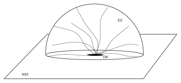
Figure 4: Here we see a hemi-spherical D2-brane ending on an NS 5-brane. $K$ D6-branes and embedded in the NS 5-brane. $K$ strings stretch to the D2-brane.

9 Giant Gravitons

One may wonder whether the Quantum Hall Soliton has an eleven dimensional meaning. Up till now we have treated the coupling constant as if it tended to a finite value at infinity. However the actual value of the asymptotic coupling cancels from all of our results concerning the behavior of the $D2$-brane. This allows us to take a limit in which the asymptotic coupling $g_{s}$ tends to infinity. This is the limit in which the 11th dimension decompactifies.

Thus the Quantum Hall solitons are naturally thought of as objects in eleven dimensions. First consider the $D6$-brane. The $11$-dimensional origin of the $D6$-brane is itself not a brane but a Kaluza Klein monopole consisting of a product of $7$-dimensional Minkowski space and a $4$-dimensional Taub-Nut space with mass parameter $K$.

Now add a graviton to this space and boost it so that its momentum along the $11$th direction is $N$ in quantized units. In the IIA description this is a configuration with a $D6$-brane and $N$ units of $D0$-brane charge. It has exactly the quantum numbers of the Quantum Hall soliton.

Ordinarily the Taub-Nut monopole will repel the graviton and send it off to transverse infinity. However our results indicate that the graviton can be trapped or bound to the center of the monopole where it will have the rich excitation spectrum of the Quantum Hall soliton.

From the results of section (2) we see that the graviton grows with increasing momentum. In this sense the soliton is similar to the giant gravitons of Ref.  [24] with the background n-form field  [25] being replaced by the Taub-Nut background.

The $11$-dimensional interpretation makes the most sense if we fix $K$ and let $N$ grow. This corresponds to boosting the graviton in a fixed background. In this case we are really discussing a fixed number of charges in the background magnetic field.

10 Conclusions

In this paper we have constructed a system of branes and strings whose low energy excitations are described in terms of non-relativistic particles moving on a $2$-sphere in a magnetic field with repulsive gauge forces between the particles. We have found that there is a characteristic energy scale for the low energy excitations and that all energies associated with the two dimensional non-relativistic system are of this scale. Thus we have all the ingredients for a string theory simulation of the Quantum Hall system.

The background magnetic field may be described in terms of a density of $D0$-branes dissolved in the $D2$-brane substrate. The $D0$-brane fluid behaves like an incompressible fluid. The $D0$-branes play the role of quantized units of flux. In this picture quasiparticles of the QH system are simply additional $D0$-branes.

Alternatively the field may be described in terms of a background $2$-form $B_{\mu\nu}$ field. More generally by choosing a gauge, the field can be represented as a combination of $D0$-branes  and $B$ flux. We argued that this gauge freedom is closely connected with the so called Composite Fermion Model of the fractional Quantum Hall Effect. Seiberg  [26] has suggested that this freedom of description may be related to the ambiguity in the definition of the $\Phi$ parameter in eq. (5.14)  [17].

We briefly discussed the modeling of edges and edge states in the system by introducing an $NS5$-brane. The $5$-brane intersects the spherical membrane along its equator and produces a boundary along with the typical chiral edge states.

A dual way of looking at the Quantum Hall Soliton is in terms of the near horizon gauge theory of a stack of $D6$-branes. From this point of view the configuration is a metastable soliton of the theory carrying $F\wedge F\wedge F$ charge. The existence of the soliton with its very rich spectrum of low energy excited states is new information about the $6$-brane.

A final point concerns compactification. In this paper we have considered the case of uncompactified $IIA$ string theory. However, we see no obstruction to compactifying the six dimensions $Y^{a}$. In this case, our configurations would exist as metastable objects in the $3+1$-dimensional world.

Needless to say, we hope that string theory techniques will be useful in understanding the Quantum Hall system and other condensed matter systems and conversely, that condensed matter phenomenology may teach us new lessons about string theory.

11 Appendix

Consider a ground string state connecting the $D6$ and $D2$ branes. General string theory arguments tell us that these strings satisfy fermionic statistics. To see this, we begin with a brane configuration in which the $D6$-brane is oriented along the $Y^{a}$ directions, $a=6,...,9$ and a $D2$-brane along the $X^{i}$ directions, $i=1,2$. The two branes may be separated along the $3$ direction.

Let us recall why the string ground state is a fermion. We are interested in the spectrum of the $6-2$ strings. The symmetry of the problem is $SO(2)\times SO(6)$. The total number of worldsheet fields which satisfy mixed boundary conditions is eight: $X^{1,2}$ satisfy $DN$ boundary conditions while the $Y^{a}$ satisfy $ND$ boundary conditions. $X^{3}$ satisfies $DD$ boundary conditions. The boundary conditions break the Lorentz symmetry in this problem.

As usual, in the $R$ sector, bosonic and fermionic fields satisfy the same periodicity conditions and the zero point energy vanishes. Therefore, in the $R$ sector the ground states are massless. The only fermionic worldsheet field that are periodic are $\Psi^{0}$ and $\Psi^{3}$. From these we get zero modes, and, therefore, an extra degenerate ground state. The two states have opposite worldsheet fermion numbers. Thus only one ground state survives the GSO projection. The surviving ground state is a singlet under the symmetry group $SO(2)\times SO(6)$.

The fact that the Ramond ground states are fermions can be deduced as follows. Let us do three $T$-dualities along the $1,2,3$-directions to turn the system into a $D1$-$D9$ brane system. $T$-duality is a gauge symmetry of the theory and should not change the spectrum or the statistics of the string states. Now let us look at the $R$ sector of the $1-9$ strings. The symmetry of the $T$-dual configuration is $SO(1,1)\times SO(8)$ and we can take advantage of this maximal symmetry. The two $R$ ground states are left and right moving spinors of $SO(1,1)$ respectively and singlets under the internal $SO(8)$. Only one of them survives the GSO projection. The fact that they are fermions follows from the spin–statistics theorem.

In the $NS$ sector, the zero point energy can be computed in the usual way giving

$$-{1\over 2}+{\#ND\over 8}={1\over 2}.$$ (11.1)

Thus the $NS$ sector is massive and therefore the bosons are massive. Separating the branes along the $3$ direction shifts the overall spectrum of the $6-2$ strings by a term proportional to the length of the stretched strings.

Finally, we remark that this configuration leaves two supersymmetries unbroken. The ground state of the $6-2$ strings is a BPS multiplet and it consists of a single state with no bose–fermi degeneracy. This state is fermionic as we have argued above. Excited states are in long multiplets and these contain equal numbers of fermions and bosons. The supersymmetry of the problem is broken by the addition of the $D0$–branes.

For the large spherical brane of section (3), we focus on a patch along the $1,2$ directions much larger than the magnetic length and approximate it as flat. Then, we can use the above analysis to estimate the free spectrum and also the statistics of the string ground state follows. As long as we focus on charged particles separated at distances of order the magnetic length, the Chern Simons term that we found in the previous section does not play any important role in the statistics.

12 Acknowledgements

L.S. would like to thank I. Klebanov, J. Maldacena, G. Moore and N. Seiberg for useful conversations. J.B. would like to thank U. Chicago for their hospitality while this work was being completed and D. Kutasov for stimulating discussions. We also acknowledge M. Fabinger, B. Freivogel, M. Kleban, J. Mcgreevy, M. Rozali, S. Shenker, E. Silverstein and S. Zhang for useful discussions. We thank A. Matusis for collaboration during the early stages of this work. The work of L.S. and N.T. was supported in part by NSF grant 980115. J.B. is supported under D.O.E. grant number AE-AC03-76SF-00515.

References

- [1] T. Banks, W. Fischler, S. H. Shenker and L. Susskind, “M theory as a matrix model: A conjecture,” Phys. Rev. D55, 5112 (1997) [hep-th/9610043].
- [2] J. Maldacena, “The large N limit of superconformal field theories and supergravity,” Adv. Theor. Math. Phys. 2, 231 (1998) [hep-th/9711200].
- [3] S. S. Gubser, I. R. Klebanov and A. M. Polyakov, “Gauge theory correlators from non-critical string theory,” Phys. Lett. B428, 105 (1998) [hep-th/9802109].
- [4] E. Witten, “Anti-de Sitter space and holography,” Adv. Theor. Math. Phys. 2, 253 (1998) [hep-th/9802150].
- [5] O. Aharony, S. S. Gubser, J. Maldacena, H. Ooguri and Y. Oz, “Large N field theories, string theory and gravity,” Phys. Rept. 323, 183 (2000) [hep-th/9905111].
- [6] E. Witten, “Anti-de Sitter space, thermal phase transition, and confinement in gauge theories,” Adv. Theor. Math. Phys. 2, 505 (1998) [hep-th/9803131].
- [7] A. Brandhuber, N. Itzhaki, J. Sonnenschein and S. Yankielowicz, “Wilson loops, confinement, and phase transitions in large N gauge theories from supergravity,” JHEP 9806, 001 (1998) [hep-th/9803263].
- [8] L. Girardello, M. Petrini, M. Porrati and A. Zaffaroni, “Confinement and condensates without fine tuning in supergravity duals of gauge theories,” JHEP 9905, 026 (1999) [hep-th/9903026].
- [9] I. R. Klebanov and M. J. Strassler, “Supergravity and a confining gauge theory: Duality cascades and (chi)SB-resolution of naked singularities,” JHEP 0008, 052 (2000) [hep-th/0007191].
- [10] S. Rey, S. Theisen and J. Yee, “Wilson-Polyakov loop at finite temperature in large N gauge theory and anti-de Sitter supergravity,” Nucl. Phys. B527, 171 (1998) [hep-th/9803135].
- [11] C. V. Johnson, A. W. Peet and J. Polchinski, “Gauge theory and the excision of repulson singularities,” Phys. Rev. D61, 086001 (2000) [hep-th/9911161].
- [12] J. Polchinski and M. J. Strassler, “The string dual of a confining four-dimensional gauge theory,” hep-th/0003136.
- [13] S. S. Gubser, “Curvature singularities: The good, the bad, and the naked,” hep-th/0002160.
- [14] S.M. Girvin, Les Houches lectures, July 1998, IUCM98-010 [cond-mat/9907002].
- [15] For an elementary account of the properties of the Quantum Hall fluid see S. Bahcall, L. Susskind, “Fluid dynamics, Chern-Simons theory and the Quantum Hall Effect,” Int. J. Mod. Phys. B5, 2735 (1991).
- [16] A. Hanany and E. Witten, “Type IIB superstrings, BPS monopoles, and three-dimensional gauge dynamics,” Nucl. Phys. B492, 152 (1997) [hep-th/9611230].
- [17] N. Seiberg, “A note on background independence in noncommutative gauge theories, matrix model and tachyon condensation,” JHEP 0009, 003 (2000) [hep-th/0008013].
- [18] A. Connes, M. R. Douglas and A. Schwarz, “Noncommutative geometry and matrix theory: Compactification on tori,” JHEP 9802, 003 (1998) [hep-th/9711162].
- [19] N. Seiberg and E. Witten, “String theory and noncommutative geometry,” JHEP 9909, 032 (1999) [hep-th/9908142].
- [20] R. B. Laughlin, “Anomalous quantum Hall effect: An incompressible quantum fluid with fractionally charged excitations,” Phys. Rev. Lett. 50, 1395 (1983).
- [21] S. Rao, “An Anyon primer,” hep-th/9209066.
- [22] B. I. Halperin, P. A. Lee and N. Read, “Theory of the half filled Landau level,” Phys. Rev. B47, 7312 (1993).
- [23] J.K. Jain, Physics Today, April 2000.
- [24] J. Mcgreevy, L. Susskind and N. Toumbas, “Invasion of the giant gravitons from anti-de Sitter space,” JHEP 0006, 008 (2000) [hep-th/0003075].
- [25] R. C. Myers, “Dielectric-branes,” JHEP 9912, 022 (1999) [hep-th/9910053].
- [26] Private communication.