From ADM to Brane-World charges

Abstract:

We first recall a covariant formalism used to compute conserved charges in gauge invariant theories. We then study the case of gravity for two different boundary conditions, namely spatial infinity and a Brane-World boundary. The new conclusion of this analysis is that the gravitational energy (and linear and angular momentum) is a local expression if our universe is really a boundary of a five-dimensional spacetime.

1 Introduction

Recently, the old idea that our real world could be a boundary of an higher dimensional spacetime has been intensively revisited after the work of Randall and Sundrum [1]. This so-called Brane-World scenario has highly non-trivial consequences on the effective four dimensional theory of gravity. In fact, the equations of motion on the brane-universe are not the usual Einstein equations in four dimensions but the modified version given in [2]. Another big difference concerns the conserved charges.

In ordinary four dimensional Einstein gravity, there is not such a notion of a local density of energy in the bulk spacetime. This is a direct consequence of the local diffeomorphism invariance. For an asymptotically flat spacetime, we can however construct a local energy density at spatial infinity, to be integrated on ${\cal B}_{\infty}$, see figure 1 (with $D=4$). This is the well known ADM mass whose construction crucially depends on the asymptotically flat boundary conditions [3].

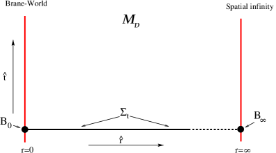
Figure 1: Spacetime bounded by one Brane-World at $r=0$, by spatial infinity at $r=\infty$ and by one Cauchy hypersurface $\Sigma_{t}$.

Let us now consider a five-dimensional spacetime bounded by one D3-brane a $r=0$ (see again figure 1 but now with $D=5$). Following the Brane-World scenario, ${\cal B}_{0}$ has to be seen as a Cauchy hypersurface of our four-dimensional universe. Now, we can of course still define an ADM mass at ${\cal B}_{\infty}$ if the five-dimensional spacetime is asymptotically flat. However, this mass cannot be measured since, by hypothesis, we are not allowed to escape from the Brane-World.

On the other hand, we can construct a measurable local density of mass at ${\cal B}_{0}$ (similar to the ADM mass at ${\cal B}_{\infty}$) using now the boundary conditions on the Brane (namely the Lanczos-Israel junction conditions). Then, although the gravitational energy is still non-local in five dimensions, we have local expressions at each boundary of this higher dimensional spacetime (namely at ${\cal B}_{0},{\cal B}_{\infty},$ or others if any). Therefore, the effective four-dimensional gravitational energy becomes localizable within ${\cal B}_{0}$ in a Brane-World scenario.

In sections 2 and 3 we recall the basic construction of conserved charges in gauge invariant theories following the references [4, 5, 6]. We then study in section 4 the case of gravity in $D$ dimensions, for the two different boundary conditions shown in figure 1. For asymptotically flat boundary conditions (namely Dirichlet boundary conditions on the metric), we recover the ADM charges, in a generally covariant form (the so-called KBL superpotential [7]) [8]. For the Lanczos-Israel boundary conditions [9] (of Neumann type on the metric), we find a new covariant expression for the Brane-World charges [10]. We finally use this expression in two very simple examples.

We skip all the details in calculations which can be found in the cited references.

2 Conserved charges associated with gauge symmetries

Let us assume that one theory is invariant under some symmetry $\delta_{\xi}\varphi^{i}$. The label ⁱ goes for all the fields present in the Lagrangian, even the auxiliary ones.

For a global symmetry, the infinitesimal parameter $\xi^{\alpha}$ is constant. The conserved charges are then given by the usual Noether construction:

$$Q_{\xi}=\int_{\Sigma_{t}}J^{\mu}_{\xi}\hat{t}_{\mu}$$ (1)

where $J^{\mu}_{\xi}$ denotes the associated Noether current and $\hat{t}_{\mu}$ the normal to the Cauchy hypersurface $\Sigma_{t}$.

For a local or gauge symmetry, (that is, $\xi^{\alpha}=\xi^{\alpha}(x)$), the formula (1) is modified by:

$$Q_{\xi}=\int_{{\cal{B}}_{r}}U^{\mu\nu}_{\xi}\hat{t}_{\mu}\hat{r}_{\nu}$$ (2)

for $r=0$ or $\infty$; see figure 1. We also denoted by $\hat{t}_{\mu}$ and $\hat{r}_{\nu}$ the normal vectors of ${\cal{B}}_{r}$.

The tensor $U^{\mu\nu}_{\xi}=-U^{\nu\mu}_{\xi}$ is called superpotential and therefore plays the role of the Noether current for local symmetries. Its construction will be recalled in the next section.

The important points about equation (2) are the following. The conserved charges associated with a gauge symmetry [4, 5, 6, 11]:

$\bullet$ can be computed on each boundary of spacetime ${\cal{B}}_{r}$ (for $r=0,\infty,$ or others if any; see figure 1) in a completely independent way by the formula (2);

$\bullet$ strongly depend on the boundary conditions imposed on ${\cal{B}}_{r}$;

$\bullet$ are functional of the gauge parameter $\xi^{\alpha}(x)$. Moreover, the number of conserved charges is given by the number of “non-zero” gauge symmetries $\delta_{\xi}\varphi^{i}$ compatibles with the boundary conditions on ${\cal B}_{r}$.

3 Computing the superpotential

The method presented in [5] to compute the superpotential $U^{\mu\nu}_{\xi}$ (2) can be summarized by the following “recipe”:

i) The theory should be reformulated in a first order form:

$$\frac{\delta{\cal L}}{\delta\varphi^{i}} =: E_{i}=E_{i}(\varphi,\partial_{\mu}\varphi)$$ (3)

$$\delta_{\xi}\varphi^{i} = \partial_{\mu}\xi^{\alpha}\Delta^{\mu i}_{\alpha}(\varphi,\partial_{\mu}\varphi)+\xi^{\alpha}\Delta^{i}_{\alpha}(\varphi,\partial_{\mu}\varphi)\ \ \ \ \$$ (4)

That is, both $E_{i}$, $\Delta^{\mu i}_{\alpha}$ and $\Delta^{i}_{\alpha}$ should not depend on $\partial^{2}\varphi^{i}$, $\partial^{3}\varphi^{i}$, etc…The introduction of auxiliary fields (which are included in the ⁱ index) is usually needed. For simply [5], we also allow at most one derivative of the gauge parameter (that is, no terms in $\partial^{2}\xi$, $\partial^{3}\xi$, etc…) in the symmetry transformation laws (4).

ii) With the definitions (3) and (4), we construct the following tensor,

$$W^{\mu}_{\xi}:=\xi^{\alpha}\Delta^{\mu i}_{\alpha}E_{i},$$ (5)

which vanishes on-shell. Note that this tensor also appears in the Noether identities associated with (4), namely $\delta_{\xi}\varphi^{i}E_{i}=\partial_{\mu}W^{\mu}_{\xi}$.

iii) Then, an arbitrary variation of the superpotential, on any ${\cal B}_{r}$, should satisfy:

$$\left.\delta U^{\mu\nu}_{\xi}=-\delta\varphi^{i}\frac{\partial W_{\xi}^{\mu}}{\partial\partial_{\nu}\varphi^{i}}\right|_{on\ {\cal B}_{r}}.$$ (6)

A theorem [5] guarantees the antisymmetry in $\mu$ and $\nu$ of the rhs of equation (6).

iv) The last step is to “integrate” the equation (6). That is, to rewrite the rhs of (6) as $\delta(\mbox{\it something})$, using the boundary conditions on ${\cal B}_{r}$.

The formula (6) gives an unambiguous superpotential, up to some global “integration”-constant. Moreover, it follows from three points:

1. $\bullet$ The Noether current associated with a gauge symmetry can be rewritten as:

   $$J_{\xi}^{\mu}=W^{\mu}_{\xi}+\partial_{\nu}U_{\xi}^{\mu\nu},$$ (7)

   for some $U_{\xi}^{\mu\nu}=-U_{\xi}^{\nu\mu}$ (together with the definition (5)).

2. $\bullet$ The variational principle is satisfied on ${\cal B}_{r}$.

3. $\bullet$ The charge defined by (2) is on-shell conserved.

The first point can be proven in general [4]. It follows from the locality of the gauge symmetry considered. The second point has to be checked by hand and then imposes some restrictions on the “allowed” boundary conditions: they should be compatible with some variational principle on ${\cal B}_{r}$. The third point is required also by hand. Therefore, the charge (2) will be conserved if the basic equation (6) for the superpotential holds. The complete derivation of (6) can be found in [5, 6, 11].

The method summarized by the four above steps i)-iv) is nothing but a Lagrangian (and then explicitely covariant) version of the Regge and Teitelboim procedure [3] in Hamiltonian formalism. There exists in fact a precise correspondence between both methods, through the so-called covariant symplectic phase space formalism [12, 13]. The key point is to realize that the equation (6) contains an hidden symplectic structure. In fact a careful analysis shows that [11]:

$$\Omega_{ij}=\int_{\Sigma_{t}}\Omega^{\mu}_{ij}\hat{t}_{\mu},$$ (8)

with,

$$\Omega^{\mu}_{ij}:=\frac{\partial E_{j}}{\partial\partial_{\mu}\varphi^{i}}$$ (9)

is antisymmetric (in $i$ and $j$), closed, covariant and conserved and thus naturally defines a symplectic two-form for first order theories. Moreover, with these definitions, the basic equations (2) and (6) can be rewritten on-shell as [11]

$$\delta_{\xi}\varphi^{i}=\left[Q_{{}_{\xi}},\varphi^{i}\right]_{\Omega},$$ (10)

with,

$$\left[\ ,\ \right]_{\Omega}:=\Omega^{ij}\frac{\delta}{\delta\varphi^{i}}\frac{\delta}{\delta\varphi^{j}}.$$ (11)

We then recovered the basic Hamiltonian equation (10) which defines the conserved charge in term of the symmetry considered.

4 The example of gravity

The formula (6) can be used for any gauge symmetry. The examples of Yang-Mills, p-forms, Chern-Simons in D=2n+1 dimensions, supergravities (in first order formalisms [14]) are treated in [5, 15, 6].

The purpose of this proceeding is to report in more detail on the case of gravity for two very different boundary conditions, namely spatial infinity [8] ($r=\infty$) and a Brane-World boundary [10] ($r=0$); see figure 1.

The starting point i) of the method given in the previous section is to use a first order formulation of gravity. Two well-known possibilities can be found in the literature:

$\bullet$ the Palatani formulation, where the metric $g_{\mu\nu}$ and the torsionless connection $\Gamma^{\rho}_{\mu\nu}=\Gamma^{\rho}_{\nu\mu}$ are treated as independent fields;

$\bullet$ the Cartan-Weyl formulation, with a vielbein $e^{a}_{\mu}$ and a $so(1,D-1,\hbox to0.0pt{\rm I\hss}\mkern 3.0mu{\rm R})$ connection ${}_{\perp}\omega_{\mu\ b}^{\ a}$ being the independent fields.

In the papers [4, 8], we worked with a third possibility, namely the Affine gravity which combines both formulations in a nice way. This theory contains three fields: a metric $g^{ab}$, a vielbein $\theta^{a}_{\mu}$ (called canonical one-form) and a $gl(D,\hbox to0.0pt{\rm I\hss}\mkern 3.0mu{\rm R})$ connection $\omega_{\mu\ b}^{\ a}$ . The Palatini formalism is recovered after fixing all the internal $gl(D,\hbox to0.0pt{\rm I\hss}\mkern 3.0mu{\rm R})$ gauge symmetry with $\theta^{a}_{\mu}=\delta^{a}_{\mu}$ (the $\delta$-Kronecker symbol). On the other hand, the vielbein theory (in its first order form) follows after fixing the internal metric by $g^{ab}=\eta^{ab}$ (the flat Minkowski metric). This last choice breaks $GL(D,\hbox to0.0pt{\rm I\hss}\mkern 3.0mu{\rm R})$ down to $SO(1,D-1,\hbox to0.0pt{\rm I\hss}\mkern 3.0mu{\rm R})$, as illustrated in figure 2.

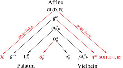
Figure 2: The Palatini and Vielbein formalisms as special cases of Affine gravity.

Using this Affine gravity (needed also for some technical reasons), we can compute the variation of the superpotential using equation (6). After going down to the Palatini formulation following the left arrows of figure 2, we find that the variation of the gravitational superpotential satisfies [8]:

$$16\pi G\ \delta U_{\xi}^{\mu\nu} = 2\ \nabla_{\rho}\xi^{\sigma}\delta\left(\sqrt{\left|g\right|}g^{\rho[\mu}\delta^{\nu]}_{\sigma}\right)$$ (12)

$$+6\ \delta\left(\Gamma^{\sigma}_{\rho\lambda}\right)\sqrt{\left|g\right|}g^{\rho[\mu}\delta^{\nu}_{\sigma}\xi^{\lambda]}\ \ \ \ \$$

The equation (12) is valid for any boundary condition of Einstein gravity (with or without cosmological constant). That means, it can be used at any ${\cal B}_{r}$. We discuss the cases of spatial infinity and of a Brane-World (namely $r=\infty$ and $r=0$, see figure 1) in the following two subsections.

4.1 “Integration” on ${\cal B}_{\infty}$: The ADM charges

The boundary conditions at spatial infinity are basically Dirichlet boundary conditions on the metric,

$$g_{\mu\nu}\stackrel{{\scriptstyle r\rightarrow\infty}}{{\longrightarrow}}\bar{g}_{\mu\nu},$$ (13)

for some given (fixed) asymptotic metric $\bar{g}_{\mu\nu}$. The two usual cases are the asymptotically flat one, $\bar{g}_{\mu\nu}=\eta_{\mu\nu}$ and the asymptotically anti-de Sitter one, $\bar{g}_{\mu\nu}=g_{\mu\nu}^{adS}$.

Using then the boundary conditions (13), we can “integrate” equation (12). The final result [8] is a $D$-dimensional version of the superpotential proposed by Katz, Bic̆ák and Lynden-Bell [7] as a covariant generalization of the ADM charges:

$$\ {}^{\mbox{\tiny\it KBL}}U_{\xi}^{\mu\nu} = \frac{\sqrt{\left|g\right|}}{16\pi G}\left(\nabla^{\mu}\xi^{\nu}-\bar{\nabla}^{\mu}\xi^{\nu}\right.$$

$$\left.+(\Delta\Gamma^{\mu}_{\rho\sigma}g^{\rho\sigma}-\Delta\Gamma^{\sigma}_{\rho\sigma}g^{\mu\rho})\xi^{\nu}\right)-\mu\leftrightarrow\nu$$

with,

$$\Delta\Gamma^{\mu}_{\rho\sigma}:=\Gamma^{\mu}_{\rho\sigma}-\bar{\Gamma}^{\mu}_{\rho\sigma},$$ (15)

and where the over-bared quantities are computed with the asymptotic bared metric $\bar{g}_{\mu\nu}$ defined through equation (13).

Note also that the result (4.1) is obtained after fixing the “integration” constant by requiring:

$$\ ^{\mbox{\tiny\it KBL}}U_{\xi}^{\mu\nu}(\bar{g}_{\mu\nu})=0$$ (16)

This condition is nothing but a normalization (or definition) of the classical zero point energy.

As in the Hamiltonian formalism, the diffeomorphism parameter $\xi^{\rho}(x)$ should be compatible with the Dirichlet boundary conditions (13):

$$g_{\mu\nu}+{\cal L}_{\xi}g_{\mu\nu}\stackrel{{\scriptstyle r\rightarrow\infty}}{{\longrightarrow}}\bar{g}_{\mu\nu}.$$ (17)

The number of non-vanishing $\xi$’s at ${\cal B}_{\infty}$ which satisfy this equation (17) gives the number of conserved charges. For instance, an infinite number of them exists in $3$-dimensional anti-de Sitter gravity (that is when $\bar{g}=g^{adS_{3}}$) [16].

In summary, using the general method recalled in section 3, we found for Dirichlet boundary conditions (13) the KBL superpotential. Moreover, this superpotential is the only one which satisfies the following properties:

$\bullet$ It is generally covariant.

$\bullet$ If the chosen coordinates are the Cartesian ones of an asymptotically flat (or anti-de Sitter) spacetime, the KBL superpotential reproduces the ADM charge formulas (or the AD [17] ones for adS).

$\bullet$ It gives the mass and angular momentum (and the conformal Brown-Henneaux [16] charges for adS₃ [6]) with the right normalization in any $D\geq 3$.

$\bullet$ It can be used at null infinity and reproduces the Bondi charges [18].

4.2 “Integration” on ${\cal B}_{0}$: The Brane-World charges

Let us start with the following Brane-World action:

$${\cal S} = \int_{{\cal M}}\frac{\sqrt{\left|g\right|}}{16\pi G}R+\int_{\partial{\cal M}}\frac{\sqrt{\left|\tilde{g}\right|}}{16\pi G}{\cal K}$$ (18)

$$+\int_{brane}{\cal L}_{brane}(\tilde{g},\varphi)$$

where ${\cal K}$ denotes the extrinsic curvature, $\tilde{g}$ the pulled-back metric on the brane and $\varphi$ some Brane-World fields.

In more general cases (basically for supergravity applications), one or several scalar fields are included in the bulk, together with some D-dimensional cosmological constant. However, it can be checked that the final result, namely equation (21), remains unchanged under these modifications [10]. That is why we consider here the simplest action (18) for illustrative purposes.

The presence of the Gibbons and Hawking [19] boundary term ${\cal K}$ in the action (18) can be explained by the following. The variational principle, namely $\delta{\cal S}=0$ (on-shell), implies the following boundary condition on the brane:

$$-\frac{\sqrt{\left|g\right|}}{16\pi G}{\cal K}_{\mu\nu}=T_{\mu\nu}^{bra}-\frac{1}{D-2}\tilde{g}_{\mu\nu}T^{bra}$$ (19)

with

$$T_{\mu\nu}^{bra}:=\frac{\delta{\cal L}_{bra}}{\delta\tilde{g}^{\mu\nu}},\ \ T^{bra}:=\tilde{g}^{\mu\nu}T_{\mu\nu}^{bra}.$$ (20)

The equation (19) is nothing but the Lanczos-Israel [9] junction condition. The link between this condition (19) and the extrinsic curvature boundary term in (18) was first pointed out in the context of four-dimensional gravity in [20] (for more recent work, see [21]). For related works from the Brane-World scenario point of view, see [22, 23, 24].

The boundary conditions (19) now fix the normal derivative of the metric. These are then Neumann conditions, in opposition to the previous Dirichlet case (13). Following the method of section 3, we can again “integrate” the basic equation (12), using now the boundary conditions (19). After several simplifications, the final expression for Brane-World charges (2) is extremely simple [10]:

$$\ ^{\mbox{\tiny BW}}Q_{\xi}=2\int_{B_{0}}\hat{T}^{bra}_{\mu\nu}t^{\mu}\xi^{\nu}$$ (21)

where $\hat{T}^{bra}_{\mu\nu}$ is “almost” the energy-momentum tensor of the brane Lagrangian (compare with (20)):

$$\hat{T}^{bra}_{\mu\nu} = T^{bra}_{\mu\nu}+\frac{1}{2}\tilde{g}_{\mu\nu}{\cal L}^{bra}$$ (22)

$$= \sqrt{\left|\tilde{g}\right|}\frac{\delta}{\delta\tilde{g}^{\mu\nu}}\left(\frac{{\cal L}_{bra}}{\sqrt{\left|\tilde{g}\right|}}\right).$$

Note that it should be possible to recover the result (21) using the Hamiltonian formalism together with the Regge and Teitelboim procedure [3].

The differences between the BW charges (21) (with (22)) and the usual energy-momentum tensor in flat spacetime are quite important:

$\bullet$ $\ {}^{\mbox{\tiny BW}}Q_{\xi}$ gives the total energy (for $\xi^{\mu}=t^{\mu}$), including the gravitational contribution. Therefore, if our real world is a Brane-World, the gravitational energy can be localized, with a covariant local density given by (22).

$\bullet$ $\ {}^{\mbox{\tiny BW}}Q_{\xi}$ vanishes if the Brane-Lagrangian depends on the pulled-back metric only through an overall $\sqrt{\left|\tilde{g}\right|}$ factor (see the examples below).

$\bullet$ The positivity of total energy would require a modified energy condition, namely:

$$\hat{T}_{\mu\nu}^{bra}t^{\mu}\xi^{\nu}\geq 0,\ \mbox{\it for }\xi^{\nu}\ \mbox{\it timelike.}$$ (23)

We will finish with a simple example where the formula (21) can be tested. Let us consider the action (18) together with a bulk scalar field:

$$-\int_{\cal M}\sqrt{\left|g\right|}\left(\frac{1}{2}g^{\mu\nu}\partial_{\mu}\phi\partial_{\nu}\phi+V(\phi)\right).$$ (24)

As we commented after equation (18), the result (21) is unchanged by the addition of the action (24). This is proven in detail in [10].

We will study the simplest example where the Brane-Lagrangian is a cosmological constant,

$$\int_{brane}\frac{\sqrt{\left|\tilde{g}\right|}}{2}\lambda(\phi),$$ (25)

together with the ansätze,

$$ds^{2} = e^{2A(r)}\eta_{ij}dx^{i}dx^{j}+dr^{2}$$ (26)

$$\phi = \phi(r)$$ (27)

for the bulk metric and the scalar field. This simple model is studied in detail in several papers, see for instance [25, 26, 27].

Using now (25) in our result (21), we immediately find that the Brane-World charges vanish:

$$\ ^{BW}Q_{\xi}=0.$$ (28)

In particular, the energy is zero. There is another independent way to recover this result. In fact, in the static case (26), we expect to find an agreement between the energy density and minus the total Lagrangian. This is indeed the case when the Gibbons-Hawking boundary term ${\cal K}$ of (18) is properly taken into account. Using the equations (25) and (26-27) in (18) and (24), we find:

$${\cal H}=-{\cal L} = e^{4A}\left(5A^{\prime 2}+2A^{\prime\prime}+\frac{1}{2}\phi^{\prime 2}+V\right)$$ (29)

$$-2\partial_{r}\left(e^{4A}A^{\prime}\right)-\frac{1}{2}\partial_{r}\left(e^{4A}\lambda\right),\ \$$

where the prime (as $\partial_{r}$) denotes a differentiation with respect to $r$.

Note that the first term in the second line of (29) comes from the Gibbons-Hawking boundary term and was not considered in [25, 26, 27]. It is then straightforward to check that ${\cal H}$ indeed vanishes using the equations of motion and the boundary conditions, in agreement with (28) (see again [10] for details).

A similar conclusion arises for the Brane-World de Sitter ansatz:

$$g_{ij}^{dS}:-dt^{2}+e^{2\sqrt{\Lambda}t}(dx_{1}^{2}+dx_{2}^{2}+dx_{3}^{2})$$ (30)

The five-dimensional metric is then given by (26), together with the replacement $\eta_{ij}\rightarrow g_{ij}^{dS}$. The Brane-World Lagrangian is again (25) and so the result (28) remains unchanged. As for the previous example, the vanishing of the energy can be checked in an independent way: The ansatz (30) is not anymore static and then the Hamiltonian is now given by ${\cal H}=\pi_{\mu\nu}\dot{g}^{\mu\nu}-{\cal L}$, with $\pi_{\mu\nu}$ the canonical momenta conjugated to the metric. Using the equations of motion and the boundary conditions, it is straightforward to check that ${\cal H}$ indeed vanishes, again in agreement with (28).

Note finally that the vanishing of energy in the supersymmetric extensions was pointed out in [28].

Acknowledgments

I would like to thank the organizers and in particular B. Julia for nice discussions and collaboration in part of this work. I am also grateful to the EU TMR contract FMRX-CT96-0012 for financial support.

References

- [1] L. Randall and R. Sundrum, Phys. Rev. Lett. 83 (1999) 3370, hep-th/9905221; Phys. Rev. Lett. 83 (1999) 4690, hep-th/9906064.
- [2] T. Shiromizu, K. Maeda and M. Sasaki, Phys. Rev. D 62 (2000) 024012, gr-qc/9910076.
- [3] T. Regge and C. Teitelboim, Ann. Phys. (NY) 88 (1974) 286.
- [4] B. Julia and S. Silva, Class. and Quant. Grav. 15 (1998) 2173, gr-qc/9804029.
- [5] S. Silva, Nucl. Phys. B 558 (1999) 391, hep-th/9809109.
- [6] S. Silva, Charges et Algèbres liées aux symétries de jauge: Construction Lagrangienne en (Super)Gravités et Mécanique des fluides, Thèse de Doctorat, Septembre 99, LPT-ENS.
- [7] J. Katz, J. Bic̆ák, D. Lynden-Bell, Phys. Rev. D 55 (1997) 5957.
- [8] B. Julia and S. Silva, to appear in Class. and Quant. Grav, gr-qc/0005127.
- [9] K. Lanczos, unpublished; W. Israel, Nuovo Cim. 44B (1966) 1; Errata-ibid 48B (1967) 463.
- [10] S. Silva, Brane-World charges, hep-th/0010098.
- [11] B. Julia and S. Silva, On covariant symplectic phase space methods, in preparation.
- [12] E. Witten, Nucl. Phys. B 276 (1986) 291; C. Crnkovic and E. Witten, in “300 Years of Gravitation, eds. S.W. Hawking and W. Israel (Cambridge: Cambridge University Press) 676; C. Crnkovic, Nucl. Phys. B 288 (1987) 431; Class. and Quant. Grav. 5 (1988) 1557.
- [13] A. Ashtekar, L. Bombelli and O. Reula, in “Analysis, Geometry and Mechanics: 200 Years After Lagrange” 417, Ed. by M. Francaviglia, D. Holm, North-Holland, Amsterdam (1990).
- [14] B. Julia and S. Silva, J. High Energy Phys. 01 (2000) 026, hep-th/9911035.
- [15] M. Henneaux, B. Julia and S. Silva, Nucl. Phys. B 563 (1999) 448, hep-th/9904003.
- [16] J.D. Brown and M. Henneaux, Commun. Math. Phys. 104 (1986) 207.
- [17] L.F. Abbott and S. Deser, Nucl. Phys. B 195 (1982) 76.
- [18] J. Katz and D. Lerer, Class. and Quant. Grav. 14 (1997) 2249, gr-qc/9612025.
- [19] G.W. Gibbons and S.W. Hawking, Phys. Rev. D 15 (1977) 2752.
- [20] G. Hayward and J. Louko, Phys. Rev. D 42 (2000) 4032.
- [21] V.D. Gladush, gr-qc/0001073.
- [22] H.A. Chamblin and H.S. Reall, Nucl. Phys. B 562 (1999) 133, hep-th/9903225.
- [23] R. Dick and D. Mikulović, Phys. Lett. B 476 (2000) 363, hep-th/0001013; R. Dick, hep-th/0007063.
- [24] C. Barceló and M. Visser, gr-qc/0008008; hep-th/0009032.
- [25] K. Skenderis and P.K. Townsend, Phys. Lett. B 468 (1999) 46, hep-th/9909070.
- [26] O. DeWolfe, D.Z. Freedman, S.S. Gubser and A. Karch, Phys. Rev. D 62 (2000) 046008, hep-th/9909134.
- [27] R. Kallosh, J. High Energy Phys. 1 (2000) 001, hep-th/9912060; R. Kallosh and A. Linde, J. High Energy Phys. 2 (2000) 005, hep-th/0001071.
- [28] E. Bergshoeff, R. Kallosh and A. Van Proeyen, hep-th/0007044.