CENTER VORTICES IN CONTINUUM YANG-MILLS THEORY

Abstract

The properties of center vortices are discussed within continuum Yang-Mills theory. By starting from the lattice theory and carefully performing the continuum limit the gauge potential of center vortices is obtained and the continuum analog of the maximal center gauge fixing is extracted. It is shown, that the Pontryagin index of center vortices is given by their self-intersection number, which vanishes unless the center vortices host magnetic monpoles, which make the vortex sheets non-oriented.

1 Introduction

At present there are two popular confinement mechanisms: the dual Meissner effect, which is based on a condensation of magnetic monopoles in the QCD vacuum, and the vortex condensation picture. Both pictures were proposed a long time ago, but only in recent years mounting evidence for the realization of these pictures has been accumulated in lattice calculations. Both pictures show up in specific partial gauge fixings.

The vortex picture of confinement, which received rather little attention after some early efforts following its inception, has recently received strong support from lattice calculations performed in the so-called maximal center gauge, where one fixes only the coset $G/Z$, but leaves the center $Z$ of the gauge group $G$ unfixed [1]. Subsequent center projection, which consists of replacing each link by its closest center element, allows the identification of the center vortex content of the gauge fields. It is found that the vortex content is a physical property of the gauge ensemble [2] and produces virtually the full Yang-Mills string tension [1]. Conversely the string tension disappears in the absence of center vortices. This property of center dominance persists at finite temperature [3] and the deconfinement phase transition can be understood in a 3-dimensional slice at a fixed spatial coordinate as a transition from a percolating vortex phase to a phase in which vortices cease to percolate [3, 4]. The vortices have also been shown to condense in the confinement phase [5]. Furthermore, in a gauge field ensemble devoid of center vortices, chiral symmetry breaking disappears and all field configurations belong to the topologically trivial sector [6]. In fact, the magnetic degrees of freedom causing confinement, monopoles and vortices, can be connected with the topological properties commonly thought to be carried by instantons.

In this lecture, I will discuss center vortices from the point of view of continuum Yang-Mills theory and study their topological properties. We will find that center vortices with non-vanishing Pontryagin index carry magnetic monopole loops. The talk is largely based on ref. [7].

2 Center vortices in continuum Yang-Mills theory

As a warming-up exercise I review how center vortices are identified in lattice gauge theory by center projection after implementing the maximal center gauge.

The lattice gauge theory is defined in terms of link variables $U_{\mu}(x)\in G$. In the maximal center gauge the gauge freedom of these link variables is exploited to bring the links $U_{\mu}(x)\in G$ as close as possible to a center element of the gauge group,

$$\sum\limits_{x,\nu}\left(trU_{\mu}(x)\right)^{2}\to max.\hskip 2.84544pt$$ (1)

For simplicity let us consider the gauge group $SU(2)$. The center is given by $Z(2)=\{1,-1\}$. The condition (1) is insensitive to a change of the sign of the link variable $U_{\mu}\to(-U_{\mu})$, which just reflects the residual $Z(2)$ symmetry. Once the maximal center gauge is implemented, center projection implies to put by hand $U_{\mu}(x)\to sign\left(trU_{\mu}(x)\right)$. After center projection, all links become center elements, that is for $SU(2)$, $U_{\mu}(x)=\pm 1$ . As a result of the center projection $D-1$ dimensional domains (hypersurfaces) $\Sigma$ of links equal to a non-trivial center element arise in a background of links given by $U_{\mu}(x)=1$, see fig. 1.

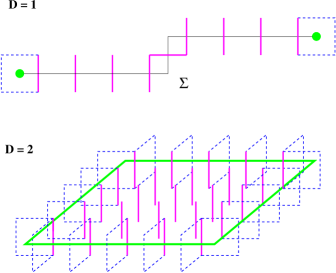
Figure 1: Illustration of non-trivial center vortex configurations arising after center projection in two and three dimensions. The full links represent non-trivial center elements forming the hypersurface $\Sigma$, the boundary $\partial\Sigma$ of which represents the center vortex

The boundaries of these hypersurfaces are given by closed $D-2$ dimensional surfaces $\partial\Sigma$, which live on the dual lattice and define an ideal center vortex. When the boundary $\partial\Sigma$ is non-trivially linked to a Wilson loop, the latter receives the corresponding non-trivial center element $Z=-1$. This can be also seen in the following way. As one travels along the loop, accumulating phases from different links making up the path, the Wilson loop stays either constant or picks up a phase corresponding to a non-trivial element of the center of the gauge group on a length of a lattice spacing. This latter change happens whenever the Wilson loops intersect the $D-1$ dimensional hypersurface $\Sigma$ describing an ideal center vortex configuration $\partial\Sigma$.

The concept of introducing center vortices by center projection can be straightforwardly extended to higher gauge groups $SU(N>2)$, for which the center elements are given by the N’th roots of unity $Z(k)=e^{i\frac{2\pi}{N}k}\hskip 2.84544pt,\hskip 2.84544ptk=0,1,\dots,N-1$. Vortices are still given by the boundaries of $D-1$ domains of links equal to a definite non-trivial center element $Z(k)$. Since for $N>2$ multiplication of non-trivial center elements can yield another non-trivial center element the possibility of center vortex fusion and fission exists. For example, for $SU(3)$ the center consists of the set of elements $\left\{z=e^{i\frac{2}{3}\pi}\hskip 2.84544pt,\hskip 2.84544ptz^{2}=e^{i\frac{4}{3}\pi}=e^{-i\frac{2}{3}\pi}\hskip 2.84544pt,\hskip 2.84544ptz^{3}=1\right\}$ and two vortices with $z(k=1)=e^{\frac{2i}{3}\pi}$ can fuse to a vortex with $z(k=2)=z(k=1)^{2}$.

Assume now, we perform an “inverse blocking”, successively replacing coarser by finer lattices. As the lattice spacing is taken to zero, these $D-1$ dimensional hypersurfaces $\Sigma$ become infinitely thin. Therefore, the continuum analogue of ideal center vortices consists in specifying $D-1$ dimensional hypersurfaces, which when intersected by a Wilson loop contribute a center element to the latter. Hence, in the continuum an explicit gauge field representation of an ideal center vortex configuration in $D$ space-time dimensions is given by

$${\cal A}_{\mu}(\Sigma,x)=E\int\limits_{\Sigma}d^{D-1}\tilde{\sigma}_{\mu}\delta^{D}\left(x-\bar{x}(\sigma)\right)\hskip 2.84544pt,$$ (2)

where $\bar{x}_{\mu}(\sigma)=\bar{x}_{\mu}\left(\sigma_{1},\dots\sigma_{D-1}\right)$ denotes a parametrization of the $D-1$ dimensional hypersurface $\Sigma$ and $d^{D-1}\tilde{\sigma}_{\mu}$ is the dual of the $D-1$ dimensional volume element. Furthermore $E$ denotes a co-weight vector, which lives in the Cartan subalgebra $E=E_{a_{0}}T_{a_{0}}$ and is defined by

$$E^{-E(k)}=Z(k)\in Z(N)\hskip 2.84544pt,\hskip 2.84544ptk=1,\dots,N-1\hskip 2.84544pt$$ (3)

where the $Z(k)$ denote the center elements of the gauge group $SU(N)$ given by the N’th roots of unity. (Thick analogs of such configurations have been considered in ref. [11].)

Calculating the Wilson loop for the gauge field (2) one obtains

$$e^{-\oint\limits_{C}{\cal A}(\Sigma)}=e^{-EI(C,\Sigma)}=Z^{I(C,\Sigma)}\hskip 2.84544pt,$$ (4)

where

$$I(C,\Sigma)=\oint\limits_{C}dx_{\mu}\oint\limits_{\Sigma}d^{D-1}\tilde{\sigma}_{\mu}\delta^{D}\left(x-\bar{x}(\sigma)\right)$$ (5)

denotes the intersection number between the loop $C$ and the hypersurface $\Sigma$. To obtain the last relation, we have used eq. (3). Eq. (4) can be used as gauge invariant definition of center vortices. In the following we will refer to the gauge field defined in eq. (2) as ideal center vortex. One should emphasize, that the precise position of the open hypersurface $\Sigma$ is irrelevant for the value of the Wilson loop. This is because the intersection number $I(C,\Sigma)$ (5) equals the linking number $L(C,\partial\Sigma)$ between the loop $C$ and the boundary $\partial\Sigma$, which represents the position of the magnetic flux of the vortex. In fact, the open hypersurface $\Sigma$ can be deformed arbitrarily by (singular) gauge transformations keeping, however, its boundary $\partial\Sigma$ fixed.

Whether the flux of a center vortex is electric or magnetic depends on the position of the $D-2$ dimensional vortex surfaces $\partial\Sigma$ in $D$-dimensional space. For example in $D=4$ the center vortex defined by the boundary of a purely spatial 3-dimensional volume $\Sigma$ carries only electric flux, which is directed normal to vortex surface $\partial\Sigma$. On the other hand a vortex $\partial\Sigma$ defined by a hypersurface $\Sigma$ evolving in time represents at fixed time, a closed loop and carries magnetic flux, which is tangential to vortex loop, see fig. 2.

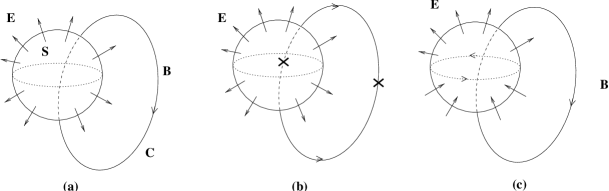
Figure 2: Three-dimensional slice of two intersecting vortex surfaces in four space-time dimensions. (a) globally oriented vortex surfaces, (b) the vortex loop evolving in the fourth dimension consists of two oppositely oriented patches connected by magnetic monopoles, (c) the vortex sphere consists of two oppositely oriented hemispheres connected by a monopole loop. (see text)

Consider the gauge transformation $V(\Sigma,x)=exp\left(-E\Omega(\Sigma,x)\right)$ defined by the solid angle $\Omega(\Sigma,x)$ subtended by the $D-1$ dimensional hypersurface $\Sigma$ from the point $x$. When $x$ crosses the hypersurface $\Sigma$, the solid angle $\Omega(\Sigma,x)$ changes by an integer and accordingly the gauge function $V$ changes by a center element $V\to ZV$, but $V$ is smooth otherwise. In particular, one should note that the derivative of $V$ along a path normal to $\Sigma$ is the same before and after the discontinuity at $\Sigma$. Indeed , one can show that

$$V(\Sigma)\partial V^{\dagger}(\Sigma)={\cal A}(\Sigma)-a(\partial\Sigma)\hskip 2.84544pt,$$ (6)

where

$$a_{\mu}(\partial\Sigma,x)=-E\int\limits_{\partial\Sigma}d^{D-2}\tilde{\sigma}_{\mu\nu}\partial^{\bar{x}}_{\nu}D\left(x-\bar{x}(\sigma)\right)$$ (7)

represents a vortex which carries the same flux (located on $\partial\Sigma$) as ${\cal A}(\Sigma,x)$. Indeed for any closed loop $C$ one has

$$\oint\limits_{C}dx_{\mu}a_{\mu}(\partial\Sigma,x)=EL(C,\partial\Sigma)\hskip 2.84544pt$$ (8)

with $L(C,\partial\Sigma)$ being the linking number between the loop $C$ and the boundary $\partial\Sigma$. Any Wilson loop is the same for the ideal center vortex ${\cal A}(\Sigma,x)$ and $a(\partial\Sigma,x)$, which is referred to in the following as thin center vortex. One can also show that the thin center vortex $a(\partial\Sigma,x)$ is the transversal part of the ideal center vortex

$$a_{\mu}(\partial\Sigma,x)=P_{\mu\nu}{\cal A}_{\nu}(\Sigma,x)\hskip 2.84544pt,\hskip 2.84544ptP_{\mu\nu}=\delta_{\mu\nu}-\frac{\partial_{\mu}\partial_{\nu}}{\partial^{2}}\hskip 2.84544pt.$$ (9)

Obviously, the thin center vortex eq. (7) manifestly depends only on the boundary $\partial\Sigma$, where the flux associated with the vortex is located.

As an illustration consider the magnetic flux of an infinitely thin and long solenoid, which represents a vortex if its magnetic flux is appropriately quantized. If we put the vortex on the $z$-axis the corresponding thin vortex gauge potential is given by

$$a(\partial\Sigma,x)=E\frac{1}{\rho}\vec{e}_{\varphi}\hskip 2.84544pt,\hskip 2.84544pt\rho=\sqrt{x^{2}+y^{2}}\hskip 2.84544pt,\hskip 2.84544pt\varphi=\arctan\frac{y}{x}\hskip 2.84544pt.$$ (10)

A related ideal vortex gauge potential is, for example, given by

$${\cal A}(\Sigma,x)=E\vec{e}_{y}\delta(y)\Theta(x)\hskip 2.84544pt,$$ (11)

which has support only on the positive $x$-axis, but yields the same value for Wilson loops as the thin vortex.

We are now in a position to present the continuum analogue of the maximal center gauge. If one represents the link variables $U_{\mu}(x)$ in the standard fashion by a gauge potential $U_{\mu}(x)=\exp\left(-aA_{\mu}(x)\right)$ and takes the naive continuum limit $a\to 0$ the maximal center gauge condition reduces to $-\int trA^{2}\to\min$, which results in the Lorentz gauge $\partial A=0\hskip 2.84544pt.$ This result is, however, wrong, since it relies on the expansion of the link variables in powers of the lattice spacing around unity $U_{\mu}(x)=1-aA_{\mu}(x)+\dots$, which is not justified if the link is close to a non-trivial center element (for example, $U_{\mu}=-1$ for $SU(2)$). Even if the lattice spacing $a$ is made smaller and smaller, during the process of gauge fixing, some of the links, initially close to unity, are rotated to group elements close to a non-trivial center element, for which the expansion around $U_{\mu}=1$ fails.

A careful analysis [7] shows that the continuum analogue of the maximal center gauge condition is given by

$$-\min\limits_{\partial\Sigma}\min\limits_{g}\int tr\left(A^{g}-a(\partial\Sigma)\right)^{2}\hskip 2.84544pt,$$ (12)

where the minimization has to be performed with respect to all continuum gauge transformations $g$ and to all vortex sheets $\partial\Sigma$. As the result of this double minimization procedure, a given gauge potential $A$ is brought as close as possible to a thin center vortex $a(\partial\Sigma)$. In this sense the maximal center gauge in the continuum theory represents a “maximal vortex gauge”.

For a fixed vortex sheet $\partial\Sigma$ minimization with respect to the gauge group yields the condition

$$\left[\partial+a(\partial\Sigma),A\right]=0\hskip 2.84544pt,$$ (13)

which is the background gauge fixing with the thin vortex $a(\partial\Sigma)$ figuring as background field.

3 Topology of center vortices

There is an essential difference between the center vortices on the lattice and in the continuum theory. After center projection on the lattice, the direction of the magnetic flux of the vortex is lost, while in the continuum theory the center vortices are given by oriented (patches of) surfaces, where the flux direction is defined by the orientation of the surfaces. The orientation of the vortices, however, is crucial for their topological properties as will be shown later.

A closed vortex surface $\partial\Sigma$ need not be globally oriented but can consist of several oriented patches $S_{k}$, $\partial\Sigma=\bigcup\limits_{k}S_{k}$ . Furthermore, these patches will in general carry flux corresponding to different non-trivial center elements, that is to different co-weight vectors $E$. We will now see that the boundaries between different oriented vortex patches host magnetic monopole loop currents. Let us first illustrate this in $D=3$.

Consider an ordinary magnetic monopole and an anti-monopole, which are connected by a Dirac string, see fig. 3.

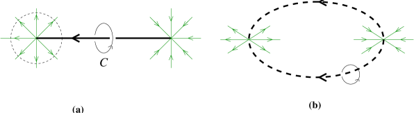
Figure 3: Illustration of the connection between Dirac string (a) and center vortex (b) (see text)

Since the Dirac string is a gauge artifact, it has to be invisible for any Wilson loop, i.e. contribute unity to the Wilson loop, just like a vanishing gauge potential. This must hold, in particular, for loops non-trivially linked to the Dirac string, which requires the magnetic flux contained in the Dirac string to be quantized in multiples of $2\pi i$

$$\phi=\int\limits_{S}d\vec{\sigma}\vec{B}=\oint\limits_{\partial S=C}d\vec{x}\vec{A}=2\pi i\hskip 2.84544pt,$$ (14)

such that $e^{-\phi}=1$ . This is the usual Dirac quantization condition. In fact the magnetic flux through a sphere $S_{2}$ around the monopole position (excluding from $S_{2}$ the piercing point of the Dirac string) is the same as the flux of the Dirac string flowing into the monopole. Hence quantization of the flux of the Dirac string implies the quantization of the magnetic charge of the monopole.

Assume now that the magnetic flux of the Dirac string is split into two equal portions, see fig. 3 . The half Dirac string carries the flux $\phi/2=\pi$ and hence contributes $e^{-i\pi}=(-1)$ to a Wilson loop non-trivially linked to it. This is the “largest” contribution a field configuration can contribute to the Wilson loop (in the sense that $-1$ is the phase which has the largest distance from the trivial phase $1$). The half Dirac string, obviously, represents a center vortex. By splitting the Dirac string into two strings of half flux, we have created a center vortex. This center vortex consists of two strings, which are connected by magnetic monopoles. The crucial point is, that at the monopole position, the direction of the magnetic flux (that is the orientation of the vortex) is reversed. This feature will survive in $D=4$, where vortices are closed sheets and magnetic monopoles move on closed loops.

The reversal of the orientation on the vortex sheet by magnetic monopole loops can also be seen in an alternative way: The vortex line (sheet) with reversed orientations can be also interpreted as an oriented vortex covered with an oppositely directed (open) Dirac string (sheet). This is because the Dirac string (sheet) carries twice the flux of a center vortex. The boundary of the open Dirac string world sheet represents the word line of a Dirac magnetic monopole (that is having a magnetic charge in accord with Dirac’s quantization condition).

In this way non-oriented closed magnetic vortex sheets consist of oriented surface pieces joined by magnetic monopole current loops. Such a non-oriented closed magnetic sheet defines a center vortex, which still gives the same contribution to a Wilson loop as the corresponding oriented vortex (in the absence of a monopole loop). Thus for the confinement properties measured by the Wilson loop, the orientation of the vortex sheet and hence the magnetic monopole currents are irrelevant. The Abelian magnetic monopole currents are, however, necessary in order to generate a non-vanishing Pontryagin index for vortex configurations as will be shown below.

The gauge fields can be topologically classified by the Pontryagin index (second Chern class)

$$\nu[A]=-\frac{1}{16\pi^{2}}\int d^{4}xtrF_{\mu\nu}\tilde{F}_{\mu\nu}=\frac{1}{4\pi^{2}}\int d^{4}xE^{a}_{i}B^{a}_{i}\hskip 2.84544pt,$$ (15)

where $E^{a}_{i}=F^{a}_{i0}$ and $B^{a}_{i}=\frac{1}{2}\epsilon_{ijk}F^{a}_{jk}$ are the corresponding colour electric and magnetic fields. From the above relation it is clear that topologically non-trivial center vortices with $\nu\neq 0$ have to carry both electric and magnetic flux. Furthermore, it is also easy to see that magnetic monopole currents are absolutely necessary on the Abelian center vortex sheet in order to generate a non-vanishing Pontryagin index. In fact, using the definition of the vortex field strength in terms of the ideal center vortex gauge potential ${\cal A}_{\mu}(\Sigma,x)$, ${\cal F}_{\mu\nu}(\partial\Sigma)=\partial_{\mu}{\cal A}_{\nu}(\Sigma)-\partial_{\nu}{\cal A}_{\mu}(\Sigma)$ and performing a partial integration, one obtains

$$\nu=-\frac{1}{8\pi^{2}}\int\limits_{M}\partial_{\mu}tr\left({\cal A}_{\nu}\tilde{{\cal F}}_{\mu\nu}\right)+\frac{1}{8\pi^{2}}\int\limits_{M}tr\left({\cal A}_{\nu}\partial_{\mu}\tilde{{\cal F}}_{\mu\nu}(\partial\Sigma)\right)\hskip 2.84544pt.$$ (16)

Using Gauss’ law in the first term and the definition of the monopole current, $j^{m}_{\mu}=\partial_{\nu}\tilde{{\cal F}}_{\mu\nu}$, in the second one, we obtain

$$\nu = -\frac{1}{8\pi^{2}}\int\limits_{\partial{\cal M}}d\sigma_{\mu}tr\left({\cal A}_{\nu}{\cal F}_{\mu\nu}\right)+\frac{1}{8\pi^{2}}\int\limits_{\cal M}tr\left({\cal A}_{\nu}j^{m}_{\nu}\right)$$ (17)

$$\equiv \nu^{(1)}+\nu^{(2)}\hskip 2.84544pt.$$

The surface term $\nu^{(1)}$ vanishes unless the integrand contains singularities, which give rise to internal surfaces wrapping the singularities. Such internal surfaces precisely arise in the presence of magnetic charges, which may be magnetic monopoles or more extended magnetic charge distributions such as line or surface charges. The second term can be cast into the form $\nu^{(2)}=-\frac{1}{4}L(\partial\Sigma,C)$ where $L(\partial\Sigma,C)$ is the linking number between the vortex surface $\partial\Sigma$ and the monopole loop $C$. This shows that a non-zero Pontryagin index indeed requires the existence of magnetic charges in the Abelian projected configurations, to which the center vortices introduced above belong.

An alternative expression for the Pontryagin index of center vortex sheets, which does not make explicit reference to magnetic monopoles, can be obtained by inserting the explicit expression for the field strength of a center vortex, ${\cal F}_{\mu\nu}(S)=E\int\limits_{S}d^{2}\sigma_{\mu\nu}\delta^{4}\left(x-\bar{x}(\sigma)\right)$ into eq. (15). Using (for $SU(2)$) $tr(EE)=-2\pi^{2}$, one finds immediately

$$\nu\left[{\cal A}(\Sigma)\right]=\nu\left[a(\partial\Sigma)\right]=\frac{1}{4}I(\partial\Sigma,\partial\Sigma)\hskip 2.84544pt,$$ (18)

where

$$I(S_{1},S_{2})=\frac{1}{2}\int\limits_{S_{1}}d^{2}\tilde{\sigma}_{\mu\nu}\int d^{2}\sigma^{\prime}_{\mu\nu}\delta^{4}\left(\bar{x}(\sigma)-\bar{x}(\sigma^{\prime})\right)$$ (19)

is the oriented intersection number between two 2-dimensional (in general open) surfaces $S_{1},S_{2}$ in $R^{4}$. From its definition, it follows that (in $D=4$) $I(S_{2},S_{1})=I(S_{1},S_{2})$. Generically two 2-dimensional surfaces intersect in $R^{4}$ at isolated points. Obviously the (self-)intersection number $I\left(\partial\Sigma,\partial\Sigma\right)$ receives contributions only from those points $\bar{x}(\sigma)=\bar{x}(\sigma^{\prime})$ where the intersecting surface patches give rise to four linearly independent tangent vectors (otherwise $d\sigma_{\mu\nu}d\tilde{\sigma}_{\mu\nu}=0$). Such points will be referred to as singular points. One can distinguish two principally different types of singular points [7, 8]:

1. transversal intersection points, for which $x(\sigma)=\bar{x}(\sigma^{\prime})\hskip 2.84544pt{\rm and}\hskip 2.84544pt\sigma\neq\sigma^{\prime}$

2. twisting (or writhing) points $\bar{x}(\sigma)=\bar{x}(\sigma^{\prime})\hskip 2.84544pt{\rm and}\hskip 2.84544pt\sigma=\sigma^{\prime}$

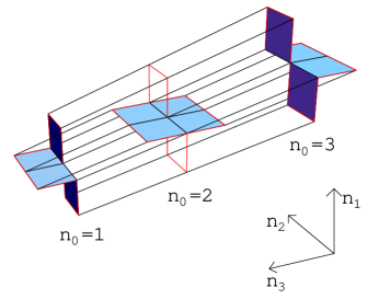
Figure 4: Sample vortex surface configuration, composed of elementary squares on a hypercubic lattice. At each (lattice) time $n_{0}$, shaded plaquettes are part of the vortex surface. These plaquettes are furthermore connected to plaquettes running in time direction; their location can be inferred most easily by keeping in mind that each link of the configuration is connected to exactly two plaquettes (i.e. the surface is closed and contains no intersection lines). Note that the two non-shaded plaquettes at $n_{0}=2$ are not part of the vortex; only the two sets of three links bounding them are. These are slices at $n_{0}=2$ of surface segments running in time direction from $n_{0}=1$ through to $n_{0}=3$. Sliced at $n_{0}=2$, these surface segments show up as lines. Furthermore, by successively assigning orientations to all plaquettes, one can convince oneself that the configuration is orientable.

Examples of the singular points of a lattice realization of a vortex sheet are given in figure 4 [8]. The surface in figure 4 is closed, orientable, has one genuine self-intersection point (precisely at the center of the configuration). Additionally, it has twisting (or writhing) points, at $n_{0}=1$ and $n_{0}=3$ in Fig. 4, as well as at $n_{0}=2$ at the front and back edges of the configuration (from the viewer’s perspective).

Transversal intersection points yield a contribution $\pm 1$ to the (oriented) intersection number, where the sign depends on the relative orientation of the two intersecting pieces. (This is easily seen by considering the intersection of two orthogonal intersecting planes.) Twisting (or writhing) points yield positive or negative contributions of modulus smaller than one to the self-intersection number.

It is well-known in topology that the self-intersection number of closed 2-dimensional surfaces in $R^{4}$ is a multiple of 4, so that the Pontryagin index (18) is indeed integer valued. It is also known that the self-intersection number of closed globally oriented 2-dimensional surfaces in $R^{4}$ vanishes. This implies that the Pontryagin index vanishes for globally oriented vortex surfaces. Consequently non-orientedness of the vortex surfaces is crucial for generating a non-vanishing Pontryagin index. To illustrate this, consider the following 3-dimensional slice of two intersecting $SU(2)$ vortex surfaces in $D=4$ dimensions, cf. fig. 2. Let the one vortex be located entirely within the spatial 3-dimensional slice of our 4-dimensional space-time manifold. It is therefore visible as a closed surface $S$, namely the sphere in fig. 2. On the other hand, let the other vortex extend into the time dimension not displayed in fig. 2. At a fixed time, it is then visible in 3-space as a closed loop $C$. Let $C$ intersect $S$ at two points as shown in fig. 2. If $S$ and $C$ are both globally oriented as in fig. 2 a, the (oriented) intersection number (in $D=3$) vanishes, since the two intersection points occur with opposite relative orientation between the intersecting manifolds. Thus, a non-zero intersection number requires at least one of the two intersecting closed manifolds to be not globally oriented. Globally non-oriented surfaces consist nevertheless of oriented patches. Assume for example the sphere $S$ in fig. 2 c to consist of two hemispheres of opposite orientation connected by a monopole loop. In this case the contributions to the oriented intersection number from the two intersection points no longer cancel but add, giving an intersection number of two.

It should come as no surprise that the magnetic monopoles are required to endow the vortex sheets with a non-trivial topological structure. This is because in certain Abelian gauges, the Pontryagin index can be expressed entirely in terms of magnetic charges. Let us consider for example the Polyakov gauge, where one diagonalizes the Polyakov line

$$\Omega(\vec{x})=\exp\left(-\int\limits dx_{0}A_{0}(x)\right)=V^{\dagger}(x)\omega(x)V(x)\to\omega(x)\hskip 2.84544pt$$ (20)

by performing the gauge transformation $A\to A^{V}=VaV^{\dagger}+V\partial V^{\dagger}$ with the coset matrix $V\in SU(2)/U(1)$. At those isolated points in space $\vec{x}_{i}$ where the Polyakov line becomes a center element $\Omega(\vec{x}_{i})=(-1)^{n_{i}}\in Z(2)$, the inhomogeneous part of the gauge transformed field $V\partial V^{\dagger}$ develops a magnetic monopole, whose charge is topologically quantized and given by the winding number $m[V]\in\pi_{2}\left(SU(2)/U(1)\right)$ of the mapping $V(\vec{x})$ from $S_{2}$ around the magnetic monopole at $\vec{x}_{i}$ into the coset $SU(2)/U(1)\sim S_{2}$. The Pontryagin index is then given by the exact relation

$$\nu=\sum\limits_{i}n_{i}m_{i}\hskip 2.84544pt,$$ (21)

where the sum runs over all magnetic monopoles. This relation was first derived in ref. [9] and was later rederived in [10].

4 Concluding remarks

The topological properties of center vortices discussed in this talk are directly relevant for an understanding of the anomalous generation of the $\eta^{\prime}$ mass within the vortex picture of the QCD vacuum, since this mass is determined by the topological susceptibility through the Witten-Veneziano formula. Furthermore, these topological properties are likely to play a role in the spontaneous breaking of chiral symmetry, in analogy to the arguments advanced in the framework of instanton models. To explain these phenomena, it is necessary to study the occurence of the various intersection points within the vortex ensemble [8]. Since these intersection points carry non-trivial topological charge, by the Atiyah-Singer index theorem, they should give rise to fermionic zero modes, which within the instanton picture of the QCD vacuum have proven responsible for the spontanous breaking of chiral symmetry. In view of the lattice result, which shows that the quark condensate disappears when the center vortices are removed [6], it is our strong belief that the vortex picture cannot only give an appealing picture of confinement and the deconfinement phase transition, but at the same time can provide an understanding of spontaneous breaking of chiral symmetry and the emergence of the topological susceptibility.

References

References

- [1] L. Del Debbio, M. Faber, J. Greensite and Š. Olejnik, Phys. Rev. D55 (1997) 2298
-
[2]
K. Langfeld, H. Reinhardt and O. Tennert, Phys. Lett. B419
(1998) 317
M. Engelhardt, K. Langfeld, H. Reinhardt, O. Tennert, Phys. Lett. B431 (1998) 141 -
[3]
K. Langfeld, O. Tennert, M. Engelhardt, H. Reinhardt, Phys. Lett.
B452 (1999) 301
M. Engelhardt, K. Langfeld, H. Reinhardt, O. Tennert, Phys. Rev. D61 (2000) 054504 - [4] M. Engelhardt, H. Reinhardt, hep-lat/9912003
- [5] T. Kovacs and E. Tomboulis, hep-lat/0002004
- [6] Ph. de Forcrand, M. D’Elia, Phys. Rev. Lett. 82 (1999) 4582
- [7] M. Engelhardt, H. Reinhardt, Nucl. Phys. B567 (2000) 249
- [8] M. Engelhardt, hep-lat/0004013
- [9] H. Reinhardt, Nucl. Phys. B503 (1997) 505
-
[10]
C. Ford, U.G. Mitreuter, T. Tok, A. Wipf, J.M. Pawlowski, Ann.
Phys. 269 (1998) 26
O. Jahn, F. Lenz, Phys. Rev. D58 (1998) 085006
M. Quandt, H. Reinhardt, A. Schaefke, Phys. Lett. B446 (1999) 290 - [11] J. M. Cornwall, Phys. Rev. D59 (1999) 125015