KEK-TH 716

hep-th/0010006

Topological Charge of $U(1)$ Instantons

on Noncommutative ${\bf{R}}^{4}$
Furuuchi  Kazuyuki

Laboratory for Particle and Nuclear Physics,
High Energy Accelerator Research Organization (KEK),
Tsukuba, Ibaraki 305-0801, Japan

Fax : (81)298-64-5755

E-mail: furuuchi@ccthmail.kek.jp

Abstract

Non-singular instantons are shown to exist on noncommutative ${\bf{R}}^{4}$ even with a $U(1)$ gauge group. Their existence is primarily due to the noncommutativity of the space. The relation between $U(1)$ instantons on noncommutative ${\bf{R}}^{4}$ and the projection operators acting on the representation space of the noncommutative coordinates is reviewed. The integer number of instantons on the noncommutative ${\bf{R}}^{4}$ can be understood as the winding number of the $U(1)$ gauge field as well as the dimension of the projection on the representation space.

1 Introduction

The concept of smooth space-time manifold must be modified at the Plunk scale due to the quantum fluctuations, and quantum gravity must explain such space-time far from being smooth. Quantum field theory on noncommutative space is expected to provide a model for the short scale structure of quantum gravity, since it has non-locality which becomes relevant at the scale introduced by the noncommutativity. The discovery of noncommutative field theory in certain limit of string theory [1] also gives concrete motivations for this subject.

Solitons and instantons play important roles in the nonperturbative analysis of quantum field theories. Noncommutativity of space introduces new ingredients to the short scale behaviour of the classical solitons. For example, in their pioneering work [2] Nekrasov and Schwarz showed that on noncommutative ${\bf{R}}^{4}$ non-singular instantons can exist even when the gauge group is $U(1)$. It is a typical appearance of the effect of noncommutativity because in ordinary $U(1)$ gauge theory on commutative ${\bf{R}}^{4}$, it is easily shown that non-singular instanton cannot exist: For the ordinary $U(1)$ gauge field on commutative ${\bf{R}}^{4}$, non-trivial instanton number is incompatible with the vanishing of field strength $F$ at infinity:

$$-\frac{1}{8\pi^{2}}\int_{{\bf{R}}^{4}}FF=-\frac{1}{8\pi^{2}}\int_{{\bf{R}}^{4}}d(AF)=-\frac{1}{8\pi^{2}}\int_{S^{3}_{\mbox{\tiny infinity}}}(AF)=0.$$ (1.1)

Therefore if there exists instanton, there must be a singularity which gives a new surface term other than $S^{3}$ at infinity. Then why $U(1)$ gauge field on noncommutative space can have non-trivial instanton charge ? It becomes quite puzzling after the following considerations: The difference between ordinary and noncommutative gauge theory is the multiplication of field (pointwise multiplication vs. star product) and gauge field itself is written as smooth function on ${\bf{R}}^{4}$. Actually, we can check that the explicit solution is not singular. On the other hand, naively thinking, the effect of noncommutativity should be suppressed at long distance and does not give further contribution to the surface term at infinity. So even in the noncommutative case there seems no room for the non-singular instanton. What’s wrong with above arguments ?

The answer is: Above naive expectation is wrong. The effect of noncommutativity does not vanish even at the long distance, in the case of $U(1)$ gauge theory. The reason is explained in the lectures.

The organization of the lecture notes is as follows. In section 2 we review the calculational techniques on noncommutative ${\bf{R}}^{2d}$. The operator symbol reviewed here is a fundamental tool throughout this note. Section 3 discusses the first half of the main themes in the lectures. After briefly reviewing the ADHM construction of instantons on noncommutative ${\bf{R}}^{4}$, we study explicit instanton solution and clarify the topological origin of the integral instanton number in $U(1)$ gauge theory on noncommutative ${\bf{R}}^{4}$. The relation between noncommutative $U(1)$ instantons and projection operators is also reviewed, where the projection operators act in Fock space which is a representation space of noncommutative coordinates. Section 4 discusses the latter half of the main themes in the lectures. In the framework of IIB matrix model we introduce a notion of gauge theory restricted to the subspace of the Fock space and consider the generalised gauge equivalence relation. Within this framework we show that the instanton number in $U(1)$ gauge theory is equal to the dimension of the projection operator. This gives an algebraic description for the origin of the integral instanton number. Finally we end with a summary and speculations in section 5.

2 Calculus on Noncommutative ${\bf{R}}^{2d}$

2.1 Noncommutative ${\bf{R}}^{2}$

First we consider noncommutative ${\bf{R}}^{2}$, since generalization to higher dimension is straightforward. Noncommutative ${\bf{R}}^{2}$ we shall consider is described by coordinates $\hat{x}^{\mu}$ ($\mu=1,2$) obeying the following commutation relations:

$$[\hat{x}^{1},\hat{x}^{2}]=i\theta^{12}=i\ell^{2},$$ (2.1)

where $\ell$ is a positive real constant and has dimension of length (the case $\theta^{12}<0$ can be considered in a similar manner). We introduce creation and annihilation operators by

$$a^{\dagger} \equiv \frac{1}{\sqrt{2}\,\ell}\,\hat{z},\qquad\hat{z}\equiv\hat{x}^{2}+i\hat{x}^{1},$$

$$a \equiv \frac{1}{\sqrt{2}\,\ell}\,\hat{\bar{z}},\qquad\hat{\bar{z}}\equiv\hat{x}^{2}-i\hat{x}^{1},$$ (2.2)

$$\qquad[a,a^{\dagger}]=1.$$

We realize the operators $\hat{x}^{1},\hat{x}^{2}$ in a Fock space ${\cal H}$ spanned by the basis $\left|n\right\rangle$:

$$\left|n\right\rangle\equiv\frac{1}{\sqrt{n!}}(a^{\dagger})^{n}\left|0\right\rangle,\qquad a\left|0\right\rangle=0.$$ (2.3)

The elements of ${\cal H}$ are called states or state vectors. The dual space ${\cal H}^{\dagger}$ of ${\cal H}$ is spanned by $\left\langle n\right|$,   where $\left\langle n\right|\equiv\left\langle 0\right|a^{n}\frac{1}{\sqrt{n!}},\,\left\langle 0\right|a^{\dagger}=0$. Let $\left|\,\phi\,\right\rangle=\sum_{n=0}^{\infty}\phi_{n}\left|n\right\rangle\in{\cal H}$, where $\phi_{n}$ are complex numbers. Then, the Hermite conjugate state is defined by

$$(\left|\phi\right\rangle)^{\dagger}\equiv\sum_{n=0}^{\infty}\left\langle\,n\right|\phi_{n}^{*}\quad.$$ (2.4)

The norm $||\,\left|\phi\right\rangle||\equiv\left\langle\phi\!\right.\left|\phi\right\rangle$ of the state $\left|\phi\right\rangle\in{\cal H}$ is deduced from

$$\left\langle 0\!\right.\left|0\right\rangle=1.$$ (2.5)

The Hermite conjugate operator $\hat{O}^{\dagger}$ of $\hat{O}$ is defined by $\left\langle\phi\right|\hat{O}^{\dagger}=(\hat{O}\left|\phi\right\rangle)^{\dagger},\,\forall\left|\phi\right\rangle\,\in{\cal H},\,$. The operator $\hat{O}$ is called Hermite if it satisfies $\hat{O}^{\dagger}=\hat{O}$.

The commutation relation (2.1) has an automorphisms of the form $\hat{x}^{\mu}\mapsto\hat{x}^{\mu}+y^{\mu}$ (translation), where $y^{\mu}$ is a commuting real number. We denote the Lie algebra of this group by ${\bf\underline{g}}$. These automorphismes are generated by unitary operator $U_{y}$:

$$U_{y}\equiv\exp[y^{\mu}\hat{\partial}_{\mu}],$$ (2.6)

where we have introduced derivative operator $\hat{\partial}_{\mu}$ by

$$\hat{\partial}_{\mu}\equiv iB_{\mu\nu}\hat{x}^{\nu},$$ (2.7)

where $B_{\mu\nu}$ is a inverse matrix of $\theta^{\mu\nu}$. $\hat{\partial}_{\mu}$ satisfies following commutation relations:

$$[\hat{\partial}_{\mu},\hat{x}^{\nu}]=\delta_{\mu}^{\nu},\quad[\hat{\partial}_{\mu},\hat{\partial}_{\nu}]=iB_{\mu\nu}.$$ (2.8)

One can check (cf. D.4 in appendix D)

$$U_{y}\,\hat{x}^{\mu}\,U_{y}^{\dagger}=\,\hat{x}^{\mu}+y^{\mu}.$$ (2.9)

We define derivative of operators by the action of g:

$$\partial_{\mu}\hat{O}\equiv\lim_{\delta y^{\mu}\rightarrow 0}\frac{1}{\delta y^{\mu}}\left(U_{\delta y^{\mu}}\hat{O}U_{\delta y^{\mu}}^{\dagger}-\hat{O}\right)=[\hat{\partial}_{\mu},\hat{O}].$$ (2.10)

Hence using (2.10), one can write the action of derivative on operator algebraically. The action of derivatives commutes:

$$\partial_{\mu}\partial_{\nu}\hat{O}-\partial_{\nu}\partial_{\mu}\hat{O}=[\hat{\partial}_{\mu},[\hat{\partial}_{\nu},\hat{O}]]-(\mu\leftrightarrow\nu)=0.$$ (2.11)

2.2 Operator Symbols

One can consider a one-to-one map from operators to ordinary c-number functions on ${\bf{R}}^{2}$ (operator symbols). Under this map noncommutative operator multiplication is mapped to star product. The map from operators to ordinary functions depends on operator ordering prescription. Weyl ordering is often used since it has some convenient properties. However the complex geometrical language is useful in the description of instantons, and in this case the normal ordering has some advantages. Here we review Wick symbol which corresponds to the normal ordering prescription. As far as considering noncommutative ${\bf{R}}^{2d}$, we can regard operators as fundamental objects, and regard operator symbols as mere representations. Therefore we can choose any convenient operator ordering. The important point is that since operator symbols are ordinary functions on ${\bf{R}}^{2}$, we can discuss topological properties of noncommutative instantons much in the same way as in the commutative case.

Let us consider normal ordered operator of the form

$$\hat{f}(\hat{x})=\int\frac{d^{2}k}{(2\pi)^{2}}\,\tilde{f}(k):e^{ik\hat{x}}:\,,$$ (2.12)

where $k\hat{x}\equiv k_{\mu}\hat{x}^{\mu}$. $:\,\,:$ denotes the normal ordering. For the operator valued function (2.12), the corresponding Wick symbol is defined by

$$f_{\scriptscriptstyle{N}}(x)=\int\frac{d^{2}k}{(2\pi)^{2}}\,\tilde{f}(k)\ e^{ikx}\,,$$ (2.13)

where $x^{\mu}$’s are commuting coordinates of ${\bf{R}}^{2}$. We define $\Omega_{N}$ as a map from operators to the Wick symbols:

$$\Omega_{N}(\hat{f}(\hat{x}))=f_{\scriptscriptstyle N}(x)\equiv\int\frac{d^{2}k}{(2\pi)^{2}}\left(2\pi\ell^{2}\mbox{Tr}_{\cal H}\left\{\hat{f}(\hat{x})\ :e^{-ik\hat{x}}:\right\}\right)\,e^{ikx}\quad.$$ (2.14)

Notice that from the relation $\mbox{Tr}_{\cal H}\bigl{\{}:\exp\,(ik\hat{x}):\bigr{\}}=\frac{2\pi}{\ell^{2}}\delta^{(2)}(k)$, it follows

$$2\pi\ell^{2}\mbox{Tr}_{\cal H}\,\hat{f}(\hat{x})=\int d^{2}x\,f_{\scriptscriptstyle{N}}(x).$$ (2.15)

The inverse map of $\Omega_{N}$ is given by

$$\Omega_{N}^{-1}(f(x))=\hat{f}^{\scriptscriptstyle{N}}(\hat{x})\equiv\int\frac{d^{2}k}{(2\pi)^{2}}\left(\int d^{2}xf(x)\ e^{-ikx}\right)\,:e^{ik\hat{x}}:\,.$$ (2.16)

The star product of functions (corresponds to the normal ordering) is defined by:

$$f(x)\star_{N}g(x)\equiv\Omega_{N}(\Omega_{N}^{-1}(f(x))\Omega_{N}^{-1}(g(x)))\,.$$ (2.17)

Since

$$:e^{ik\hat{x}}:\,:e^{ik\hat{x}}:=e^{-\bar{w}\hat{z}}e^{w\hat{\bar{z}}}e^{-\bar{w}^{\prime}\hat{z}}e^{w^{\prime}\hat{\bar{z}}}=e^{-\frac{\zeta}{2}w\bar{w}^{\prime}}e^{-(\bar{w}+\bar{w}^{\prime})\hat{z}}e^{(w+w^{\prime})\hat{\bar{z}}},$$ (2.18)

where

$$w=\frac{i}{2}(k_{2}+ik_{1}),$$ (2.19)

the explicit form of the star product is given by

$$f(z,\bar{z})\star_{N}g(z,\bar{z})=\left.e^{\frac{\zeta}{2}\frac{\partial}{\partial\bar{z}}\frac{\partial}{\partial{z^{\prime}}}}f(z,\bar{z})g(z^{\prime},\bar{z}^{\prime})\right|_{z^{\prime}=z,\bar{z}^{\prime}=\bar{z}}\quad.$$ (2.20)

From the definition (2.17), the star product is associative:

$$(f(x)\star_{N}g(x)\,)\star_{N}h(x)=f(x)\star_{N}(g(x)\star_{N}h(x)\,).$$ (2.21)

If we use coherent states, the expression of the normal symbol becomes simpler. The coherent state $\left|\bar{z}\right\rangle$ is an eigen state of annihilation operator $\hat{\bar{z}}$:

$$\hat{\bar{z}}\left|\bar{z}\right\rangle=\bar{z}\left|\bar{z}\right\rangle.$$ (2.22)

As a notation we write the dual state of $\left|\bar{z}\right\rangle$ as $\left\langle z\right|$ : $\left\langle z\right|a^{\dagger}=\left\langle z\right|z$. Then the Wick symbol of operator $\hat{f}$ is given by

$$f_{\scriptscriptstyle N}(z,\bar{z})=\left\langle z\right|\hat{f}\left|\bar{z}\right\rangle.$$ (2.23)

(2.23) follows from (2.12), (2.13) and

$$\left\langle z\right|:e^{ik\hat{x}}:\left|\bar{z}\right\rangle = \left\langle z\right|e^{-\bar{w}\hat{z}}e^{w\hat{\bar{z}}}\left|\bar{z}\right\rangle=e^{-\bar{w}z}e^{w\bar{z}}$$ (2.24)

$$= e^{ikx}.$$

(we have normalised the coherent states as $\left\langle z\!\right.\left|\bar{z}\right\rangle=1$). From (2.23) the Wick symbol $f_{\scriptscriptstyle N}(z,\bar{z})$ vanishes at $z=w$ when the corresponding operator $\hat{f}$ annihilates $\left|\bar{w}\right\rangle$ or $\left\langle w\right|$:

$$\hat{f}\left|\bar{w}\right\rangle=0\,\,\,\mbox{or}\,\,\left\langle w\right|\hat{f}=0\quad\Longrightarrow\quad f_{\scriptscriptstyle N}(w,\bar{w})=0.$$ (2.25)

Examples

First let us consider the projection operator to the Fock vacuum $\left|0\right\rangle$:

$$\left|0\right\rangle\left\langle 0\right|=:e^{-a^{\dagger}a}:=:e^{-\frac{2}{\ell^{2}}\hat{z}\hat{\bar{z}}}:\quad.$$ (2.26)

Corresponding Wick symbol is given by $e^{-\frac{1}{2\ell^{2}}z\bar{z}}$. Notice that this function concentrates around the origin of ${\bf{R}}^{2}$ within radius $\ell$. It is also easy to obtain

$$\Omega_{N}(\left|m\right\rangle\left\langle n\right|)=\frac{1}{\sqrt{m!}}\left(\frac{1}{\sqrt{2}\ell}z\right)^{m}e^{-\frac{2}{\ell}z\bar{z}}\left(\frac{1}{\sqrt{2}\ell}\bar{z}\right)^{n}\frac{1}{\sqrt{n!}}\quad.$$ (2.27)

The Wick symbol of the projection operator to the coherent state $\left|\bar{w}\right\rangle$ is given by

$$\Omega_{N}(\left|\bar{w}\right\rangle\left\langle w\right|)=e^{-\frac{1}{2\ell^{2}}(z-w)(\bar{z}-\bar{w})}\quad.$$ (2.28)

This function is obtained from $\Omega_{N}(\left|0\right\rangle\left\langle 0\right|)=e^{-\frac{1}{2\ell^{2}}z\bar{z}}$ by translation and concentrates around $z=w$.

2.3 Noncommutative ${\bf{R}}^{2d}$

Generalization to noncommutative ${\bf{R}}^{2d}$ may be straightforward. Coordinates on noncommutative ${\bf{R}}^{2d}$ obey the following commutation relations:

$$[\hat{x}^{i},\hat{x}^{j}]=i\theta^{ij}.$$ (2.29)

Using $SO(2d)$ rotations in ${\bf{R}}^{2d}$, we can choose the coordinates $\theta^{ij}=0$ except $\theta^{i(i+1)}=-\theta^{(i+1)i}\neq 0,i=1,\cdots d.$ We assume $\theta^{i(i+1)}>0$ ($\theta^{i(i+1)}<0$ case can be treated similarly). Then we define creation and annihilation operators by

$$\hat{z}_{i}\equiv\hat{x}_{i+1}+i\hat{x}_{i},\quad\hat{\bar{z}}_{i}\equiv\hat{x}_{i+1}-i\hat{x}_{i}.$$ (2.30)

The noncommutative ${\bf{R}}^{2d}$ is described by operators acting in the Fock space ${\cal H}$ spanned by the basis $\left|n_{1},\cdots,n_{d}\right\rangle$, where

$$\left|n_{1},\cdots,n_{d}\right\rangle\equiv\Biggl{\{}\Biggr{.}\prod_{i=1}^{d}\frac{1}{\sqrt{n_{i}!}}\left(\sqrt{\frac{1}{2\theta^{i(i+1)}}}\hat{z}_{i}\right)^{n_{i}}\Biggl{.}\Biggr{\}}\left|0,\cdots,0\right\rangle,$$

$$\hat{\bar{z}}_{i}\left|0,\cdots,0\right\rangle=0.$$ (2.31)

The correspondences between the descriptions by operators and by c-number functions are given by

$$\hat{f}=\int\frac{d^{2d}k}{(2\pi)^{2d}}\,\tilde{f}(k)\,:\,e^{ik\hat{x}}\,: \leftrightarrow f=\int\frac{d^{2d}k}{(2\pi)^{2d}}\,\tilde{f}(k)\,e^{ikx},$$

$$\hat{f}\hat{g} \leftrightarrow f\star_{N}g,$$

$$(2\pi)^{d}\sqrt{det\theta}\,\mbox{Tr}_{\cal H} \leftrightarrow \int d^{2d}x\quad.$$ (2.32)

Hereafter we will identify operator and corresponding Wick symbol by eqs. (2.3): We use same letter for operator and corresponding Wick symbol, as long as it is not confusing. For example we omit the hat $\hat{\,}$ from the noncommutative coordinate $\hat{x}^{\mu}$ in the following.

3 Topological Charge of $U(1)$ Instantons on
Noncommutative ${\bf{R}}^{4}$

3.1 Gauge Theory on Noncommutative ${\bf R}^{4}$

Now let us consider noncommutative ${\bf{R}}^{4}$. The coordinates $x^{\mu}\,\,(\mu=1,\cdots,4)$ of the noncommutative ${\bf{R}}^{4}$ obey following commutation relations:

$$[x^{\mu},x^{\nu}]=i\theta^{\mu\nu},$$ (3.1)

where $\theta^{\mu\nu}$ is real and constant. We restrict ourselves to the case where $\theta^{\mu\nu}$ is self-dual and set

$$\theta^{12}=\theta^{34}=\frac{\zeta}{4}\,\,,$$ (3.2)

for simplicity. We introduce the complex coordinates by

$$z_{1}=x_{2}+ix_{1},\quad z_{2}=x_{4}+ix_{3}\,.$$ (3.3)

Their commutation relations become

$$[z_{1},\bar{z}_{1}]=[z_{2},\bar{z}_{2}]=-\frac{\zeta}{2}\quad,\qquad\mbox{(others: zero)}.$$ (3.4)

We choose $\zeta>0$. We realize $z$ and $\bar{z}$ as creation and annihilation operators acting in a Fock space ${\cal H}$ spanned by the basis $\left|n_{1},n_{2}\right\rangle$:

$$\sqrt{\frac{2}{\zeta}}z_{1}\left|n_{1},n_{2}\right\rangle = \sqrt{n_{1}+1}\left|n_{1}+1,n_{2}\right\rangle,\quad\sqrt{\frac{2}{\zeta}}\bar{z}_{1}\left|n_{1},n_{2}\right\rangle=\sqrt{n_{1}}\left|n_{1}-1,n_{2}\right\rangle,$$

$$\sqrt{\frac{2}{\zeta}}z_{2}\left|n_{1},n_{2}\right\rangle = \sqrt{n_{2}+1}\left|n_{1},n_{2}+1\right\rangle,\quad\sqrt{\frac{2}{\zeta}}\bar{z}_{2}\left|n_{1},n_{2}\right\rangle=\sqrt{n_{2}}\left|n_{1},n_{2}-1\right\rangle.$$ (3.5)

The action of the exterior derivative $d$ to the operator $O$ is defined as:

$$dO\equiv(\partial_{\mu}O)\,dx^{\mu}.$$ (3.6)

Here $dx^{\mu}$’s are defined in a usual way, i.e. they commute with $x^{\mu}$ and anti-commute among themselves: $dx^{\mu}dx^{\nu}=-dx^{\nu}dx^{\mu}$. The covariant derivative $D$ is written as

$$D=d+A.$$ (3.7)

Here $A=A_{\mu}dx^{\mu}$ is a $U(n)$ gauge field. The field strength of $A$ is given by

$$F\equiv D^{2}=dA+A^{2}\equiv\frac{1}{2}F_{\mu\nu}dx^{\mu}dx^{\nu}.$$ (3.8)

We consider following Yang-Mills action:

$$S=\frac{1}{4g^{2}}\left(2\pi\frac{\zeta}{4}\right)^{2}\mbox{Tr}_{{\cal H}}\mbox{tr}_{U(n)}\,F_{\mu\nu}F^{\mu\nu},$$ (3.9)

or we can rewrite it using Wick symbols:

$$S=\frac{1}{4g^{2}}\int\mbox{tr}_{U(n)}\,F*F,$$ (3.10)

where $*$ is the Hodge star. In (3.10) multiplication of the fields is understood as the star product. The action (3.10) is invariant under the following $U(n)$ gauge transformation:

$$A\rightarrow UdU^{\dagger}+UAU^{\dagger}.$$ (3.11)

Here $U$ is a unitary operator:

$$UU^{\dagger}=U^{\dagger}U=\mbox{Id}_{{\cal H}}\otimes\mbox{Id}_{n}\quad.$$ (3.12)

Here $\mbox{Id}_{{\cal H}}$ is the identity operator acting in ${\cal H}$ and $\mbox{Id}_{n}$ is the $n\times n$ identity matrix. The gauge field $A$ is called anti-self-dual if its field strength obeys the following equation:

$$F^{+}\equiv\frac{1}{2}(F+*F)=0.$$ (3.13)

Anti-self-dual gauge fields minimize the Yang-Mills action (3.10). Instanton is an anti-self-dual gauge field with finite Yang-Mills action (3.10). The instanton number is defined by

$$-\frac{1}{8\pi^{2}}\int\mbox{tr}_{U(n)}\,FF\quad.$$ (3.14)

and takes integral value. In ordinary $U(2)$ gauge theory, integral instanton number can be understood topologically: It is a winding number of gauge field classified by $\pi_{3}(U(2))$. However when the gauge group is $U(1)$, the topological origin of the integral instanton number may seem unclear. In the lectures I will explain the origin of the integral instanton number in noncommutative $U(1)$ gauge theory.

3.2 ADHM Construction of Instantons on Noncommutative ${\bf{R}}^{4}$

ADHM construction is a way to obtain instanton solutions on ${\bf{R}}^{4}$ from solutions of some quadratic matrix equations [35]. It was generalized to the case of noncommutative ${\bf{R}}^{4}$ in [2]. The steps in the ADHM construction of instantons on noncommutative ${\bf{R}}^{4}$ in gauge group $U(n)$ with instanton number $k$ is as follows.

1. Matrices (entries are c-numbers):

   $$B_{1},B_{2} : k\times k\quad\mbox{complex matrices.}$$

   $$I,J^{\dagger} : k\times n\quad\mbox{complex matrices.}$$ (3.15)

2. Solve the ADHM equations

   $$\mu_{\bf{R}} = \zeta\,\mbox{Id}_{k}\qquad\mbox{(real ADHM equation)},$$ (3.16)

   $$\mu_{\bf{C}} = 0\qquad\quad\mbox{(complex ADHM equation)}.$$ (3.17)

   Here $\mu_{\bf{R}}$ and $\mu_{\bf{C}}$ are defined by

   $$\mu_{\bf{R}} \equiv [B_{1},B_{1}^{\dagger}]+[B_{2},B_{2}^{\dagger}]+II^{\dagger}-J^{\dagger}J,$$ (3.18)

   $$\mu_{\bf C} \equiv [B_{1},B_{2}]+IJ.$$ (3.19)

3. Define $2k\times(2k+n)$ matrix ${\cal D}_{z}$ :

   $${\cal D}_{z}\equiv\left(\begin{array}[]{c}\tau_{z}\\ \sigma_{z}^{\dagger}\end{array}\right),$$ (3.22)

   $$\tau_{z}\equiv(\,B_{2}-{z}_{2},\,B_{1}-{z}_{1},\,I\,),$$

   $$\sigma_{z}^{\dagger}\equiv(\,-(B_{1}^{\dagger}-\bar{{z}}_{1}),\,B_{2}^{\dagger}-\bar{{z}}_{2},\,J^{\dagger}\,).$$ (3.23)

   Here $z$’s are noncommutative operators.

4. Look for all the solutions to the equation

   $${\cal D}_{z}\Psi^{(a)}=0\quad(a=1,\ldots,n),$$ (3.24)

   where $\Psi^{(a)}$ is a $2k+n$ dimensional vector and its entries are operators:  Here we impose following normalization condition for $\Psi^{(a)}$:

   $$\Psi^{(a)\dagger}\Psi^{(b)}=\delta^{ab}\mbox{Id}_{{\cal H}}\quad.$$ (3.25)

   In the following we will call these zero-eigenvalue vectors $\Psi^{(a)}$ zero-modes.

5. Construct gauge field by the formula

   $$A^{ab}_{\mu}=\Psi^{(a)\dagger}\partial_{\mu}\Psi^{(b)},$$ (3.26)

   where $a$ and $b$ become indices of $U(n)$ gauge group. Then this gauge field is anti-self-dual.

In the proof of the anti-self-duality, following equations are important.

$$\tau_{z}\tau_{z}^{\dagger} = \sigma_{z}^{\dagger}\sigma_{z}:=\Box_{z},$$ (3.27)

$$\tau_{z}\sigma_{z} = 0,$$ (3.28)

$$\Psi^{(a)\dagger}\Psi^{(b)} = \delta^{ab}\mbox{Id}_{{\cal H}}.$$ (3.29)

The equation (3.27) is equivalent to the real ADHM equation provided that the coordinates are noncommutative as in 3.4, or more generally $[z_{1},\bar{z}_{1}]+[z_{2},\bar{z}_{2}]=-\zeta$. This is what Nekrasov and Schwarz found in their pioneering work [2]. The equation (3.28) is equivalent to the complex ADHM equation. The equation (3.29) is simple but necessary (however we can relax this condition by extending the notion of gauge equivalence. See section 4). Let us check that the field strength constructed from (3.26) is really anti-self-dual:

$$F = dA+A^{2}$$ (3.30)

$$= d(\Psi^{\dagger}d\Psi)+(\Psi^{\dagger}d\Psi)(\Psi^{\dagger}d\Psi)$$

$$= d\Psi^{\dagger}(1-\Psi\Psi^{\dagger})d\Psi.$$

In the above we have suppressed $U(n)$ indices. Here we have already used the condition (3.29). One of the key ingredients in the ADHM construction is that $(1-\Psi\Psi^{\dagger})$ is a projection acting on ${\bf{C}}^{2k+n}\otimes{\cal H}$ and project out the space of zero-modes, since $\Psi\Psi^{\dagger}$ is a projection to the space of zero-modes (because of the normalization condition (3.29)). Hence it can be rewritten as

$$1-\Psi\Psi^{\dagger} = {\cal D}_{z}^{\dagger}\frac{1}{{\cal D}_{z}{\cal D}_{z}^{\dagger}}{\cal D}_{z}\quad.$$ (3.31)

Indeed ${\cal D}_{z}^{\dagger}\frac{1}{{\cal D}_{z}{\cal D}_{z}^{\dagger}}{\cal D}_{z}$ is a projection that project out the zero-modes of ${\cal D}_{z}$:

$$\left({\cal D}_{z}^{\dagger}\frac{1}{{\cal D}_{z}{\cal D}_{z}^{\dagger}}{\cal D}_{z}\right)^{2}={\cal D}_{z}^{\dagger}\frac{1}{{\cal D}_{z}{\cal D}_{z}^{\dagger}}{\cal D}_{z}{\cal D}_{z}^{\dagger}\frac{1}{{\cal D}_{z}{\cal D}_{z}^{\dagger}}{\cal D}_{z}={\cal D}_{z}^{\dagger}\frac{1}{{\cal D}_{z}{\cal D}_{z}^{\dagger}}{\cal D}_{z}\quad.$$ (3.32)

(3.32) can be written as

$${\cal D}_{z}^{\dagger}\frac{1}{{\cal D}_{z}{\cal D}_{z}^{\dagger}}{\cal D}_{z} = \tau^{\dagger}_{z}\frac{1}{\,\tau_{z}\tau^{\dagger}_{z}}\tau_{z}+\sigma_{z}\frac{1}{\,\sigma_{z}^{\dagger}\sigma_{z}}\sigma_{z}^{\dagger}$$ (3.33)

$$= \tau^{\dagger}_{z}\frac{1}{\,\,\Box_{z}}\tau_{z}+\sigma_{z}\frac{1}{\,\,\Box_{z}}\sigma_{z}^{\dagger},$$

where we have used the notations in (3.27). Since $\tau_{z}\Psi=\sigma_{z}^{\dagger}\Psi=0$ by definition (3.24), it follows that $\tau_{z}d\Psi=-d\tau_{z}\Psi,\,\sigma_{z}^{\dagger}d\Psi=-d\sigma_{z}^{\dagger}\Psi$. Hence

$$F = d\Psi^{\dagger}(1-\Psi\Psi^{\dagger})d\Psi$$ (3.43)

$$= d\Psi^{\dagger}\left(\tau^{\dagger}_{z}\frac{1}{\,\,\Box_{z}}\tau_{z}+\sigma_{z}\frac{1}{\,\,\Box_{z}}\sigma_{z}^{\dagger}\right)d\Psi$$

$$= \Psi^{\dagger}\left(d\tau^{\dagger}_{z}\frac{1}{\,\,\Box_{z}}d\tau_{z}+d\sigma_{z}\frac{1}{\,\,\Box_{z}}d\sigma_{z}^{\dagger}\right)\Psi$$

$$= \begin{array}[]{ccc}\bigl{(}\,\psi_{1}^{\dagger}&\,\psi_{2}^{\dagger}&\,\xi^{\dagger}\,\bigr{)}\\ &&\\ &&\end{array}\!\!\left(\begin{array}[]{ccc}dz_{1}\frac{1}{\,\,\Box_{z}}d\bar{z}_{1}+d\bar{z}_{2}\frac{1}{\,\,\Box_{z}}dz_{2}&-dz_{1}\frac{1}{\,\,\Box_{z}}d\bar{z}_{2}+d\bar{z}_{2}\frac{1}{\,\,\Box_{z}}dz_{1}&0\\ -dz_{2}\frac{1}{\,\,\Box_{z}}d\bar{z}_{1}+d\bar{z}_{1}\frac{1}{\,\,\Box_{z}}dz_{2}&dz_{2}\frac{1}{\,\,\Box_{z}}d\bar{z}_{2}+d\bar{z}_{1}\frac{1}{\,\,\Box_{z}}dz_{1}&0\\ 0&0&0\end{array}\right)\left(\begin{array}[]{c}\psi_{1}\\ \psi_{2}\\ \xi\end{array}\right)$$

$$\equiv F^{-}_{\mbox{\tiny ADHM}}\quad.$$ (3.44)

where we have written

$$\Psi\equiv\left(\begin{array}[]{c}\psi_{1}\\ \psi_{2}\\ \xi\end{array}\right)\equiv\left(\begin{array}[]{ccc}&&\\ \Psi^{(1)}&\cdots&\Psi^{(n)}\\ &&\end{array}\right),\qquad\begin{array}[]{c}\psi_{1}:k\times n\,\,\mbox{matrix.}\\ \psi_{2}:k\times n\,\,\mbox{matrix.}\\ \,\,\xi\,\,:n\times n\,\,\mbox{matrix.}\end{array}$$ (3.54)

$F^{-}_{\mbox{\tiny ADHM}}$ is anti-self-dual: $F_{z_{1}\bar{z}_{1}}+F_{z_{2}\bar{z}_{2}}=0$, $F_{z_{1}z_{2}}=0$.

Now let us consider the large $r\equiv\sqrt{x^{\mu}x_{\mu}}$ behaviour of the gauge field thus constructed. From the form of ${\cal D}_{z}$ in (3.22), the asymptotic form of the zero-mode $\Psi$ becomes

$$\Psi=\left(\begin{array}[]{c}0\\ 0\\ \xi\end{array}\right)+O(r^{-1})\quad(r\rightarrow\infty).$$ (3.58)

Then the asymptotic form of the gauge field becomes

$$A_{\mu}=\xi^{\dagger}\partial_{\mu}\xi+O(r^{-2})\quad(r\rightarrow\infty).$$ (3.59)

From (3.59) we can observe that only the third factor $\xi$ of $\Psi$ is relevant for the asymptotic behaviour of the gauge field.

3.3 $U(1)$ One-Instanton Solution and Its Topological Charge

Now that we have reviewed the ADHM construction of instantons on noncommutative ${\bf{R}}^{4}$, we can construct explicit instanton solutions. The simplest solution is $U(1)$ one-instanton solution. In this case $B_{1}$ and $B_{2}$ are $1\times 1$ matrices, i.e. complex numbers. Therefore commutators with $B_{1}$ and $B_{2}$ are automatically give zero and the solution to the ADHM equation (3.18) is given by

$$\quad I=\sqrt{\zeta}\,,\quad\,J=0,$$ (3.60)

with $B_{1}$ and $B_{2}$ arbitrary. $B_{1}$ and $B_{2}$ are parameters that represent the position of instanton. Due to the translational invariance on noncommutative ${\bf{R}}^{4}$, it is enough if we consider $B_{1}=B_{2}=0$ solution. There is a solution $\tilde{\Psi}_{0}$ to the equation ${\cal D}_{z}\tilde{\Psi}_{0}=0$ :

$$\tilde{\Psi}_{0}=\left(\begin{array}[]{c}\tilde{\psi_{1}}\\ \tilde{\psi_{2}}\\ \tilde{\xi}\end{array}\right)=\left(\begin{array}[]{c}\sqrt{\zeta}\bar{z}_{2}\\ \sqrt{\zeta}\bar{z}_{1}\\ \left(z_{1}\bar{z}_{1}+z_{2}\bar{z}_{2}\right)\end{array}\right).$$ (3.67)

Notice that all the components of $\tilde{\Psi}_{0}$ annihilate $\left|0,0\right\rangle$. As a consequence $\tilde{\Psi}_{0}^{\dagger}\tilde{\Psi}_{0}=(z_{1}\bar{z}_{1}+z_{2}\bar{z}_{2})(z_{1}\bar{z}_{1}+z_{2}\bar{z}_{2}+\zeta)$ annihilates $\left|0,0\right\rangle$. This means $\tilde{\Psi}_{0}^{\dagger}\tilde{\Psi}_{0}$ does not have its inverse operator and we cannot normalize the zero-mode $\tilde{\Psi}_{0}$. This is a problem since we cannot follow the steps in ADHM construction, see eq.(3.25) and eq.(3.29). What should we do ?

The solution of this problem can be found if we notice that the dimension of the Fock space ${\cal H}$ is infinite. Before explaining the reason in the case of instanton, let us recall the famous story which shows the mysterious nature of infinity.

There was a hotel in some far place, and there was an infinite number of rooms in that hotel. One day all rooms were filled. Then a traveller who wanted to stay at that hotel came, see fig.1. Can you make another room for the traveller ? The answer may be apparent from fig.2: We require every guest to move to the next room.

Figure 1: Can you make another room for the traveller ?

Figure 2: We have a room for the travellar and now he is happy !

Tracing back this argument, we can find a solution of the problem in the case of instanton. We want to eliminate the zero-eigenvalue component of $\tilde{\Psi}_{0}^{\dagger}\tilde{\Psi}_{0}$, that is, $\left|0,0\right\rangle\left\langle 0,0\right|$. This corresponds to the empty room in fig. 2. What we should do is to find a operator $U$ which gives one-to-one map from $p{\cal H}$ to ${\cal H}$, where $p=1-\left|0,0\right\rangle\left\langle 0,0\right|$ . Such operator $U$ satisfies [9][4]

$$UU^{\dagger}=1,\quad U^{\dagger}U=p=1-\left|0,0\right\rangle\left\langle 0,0\right|.$$ (3.68)

One example of such operator $U_{1}$ is given by

$$U_{1} = (1-\left|0\right\rangle\left\langle 0\right|_{2})+\sum_{n_{1}=0}^{\infty}\left|n_{1},0\right\rangle\left\langle n_{1}+1,0\right|$$

$$= (1-\left|0\right\rangle\left\langle 0\right|_{2})+\left|0\right\rangle\left\langle 0\right|_{2}\frac{1}{\sqrt{\hat{n}_{1}+1}}a_{1},$$

where we have defined

$$\left|m\right\rangle\left\langle n\right|_{2}\equiv\sum_{n_{1}=0}^{\infty}\left|n_{1},m\right\rangle\left\langle n_{1},n\right|,$$ (3.70)

see fig.3 .

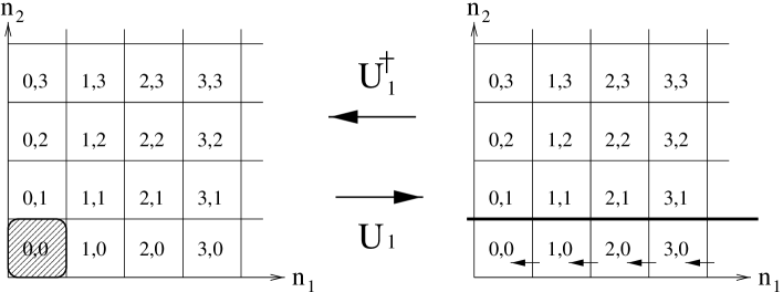
Figure 3:

To construct a zero-mode which is normalized as in (3.25), we first normalize the zero-mode $\tilde{\Psi}_{0}$ in the subspace of the Fock space where $\left|0,0\right\rangle$ is projected out:

$$\Psi_{0}\equiv\tilde{\Psi}_{0}(\tilde{\Psi}_{0}^{\dagger}\tilde{\Psi}_{0})^{-1/2}\equiv\left(\begin{array}[]{c}(\psi_{1})_{0}\\ (\psi_{2})_{0}\\ \xi_{0}\end{array}\right).$$ (3.74)

Here $(\tilde{\Psi}_{0}^{\dagger}\tilde{\Psi}_{0})^{-1/2}$ is defined in $p{\cal H}$:

$$(\tilde{\Psi}_{0}^{\dagger}\tilde{\Psi}_{0})^{-1/2}\equiv\frac{2}{\zeta}\sum_{(n_{1},n_{2})\neq(0,0)}\frac{1}{(n_{1}+n_{2})(n_{1}+n_{2}+2)}\left|n_{1},n_{2}\right\rangle\left\langle n_{1},n_{2}\right|.$$ (3.75)

Notice that (3.75) is well defined since it is defined in $p{\cal H}$ where $\left|0,0\right\rangle\left\langle 0,0\right|$ is projected out. $\Psi_{0}$ is normalized as

$$\Psi_{0}^{\dagger}\Psi_{0}=p=1-\left|0,0\right\rangle\left\langle 0,0\right|.$$ (3.76)

Then we define $\Psi$ using $U_{1}$:

$$\Psi=\Psi_{0}U_{1}^{\dagger}\quad.$$ (3.77)

$\Psi$ is normalized as in (3.25):

$$\Psi^{\dagger}\Psi=U_{1}\Psi_{0}^{\dagger}\Psi_{0}U_{1}^{\dagger}=U_{1}(1-\left|0,0\right\rangle\left\langle 0,0\right|)U_{1}^{\dagger}=1.$$ (3.78)

Hence the gauge field

$$A_{\mu}=\Psi^{\dagger}\partial_{\mu}\Psi,$$ (3.79)

is anti-self-dual.

Now let us calculate the instanton number. It is written as a surface term in the same way as in the commutative case:

$$-\frac{1}{8\pi^{2}}\int_{{\bf{R}}^{4}}FF=-\frac{1}{8\pi^{2}}\int_{{\bf{R}}^{4}}dK=-\frac{1}{8\pi^{2}}\int_{\mbox{surface at }\infty}K.$$ (3.80)

Here

$$K\equiv AdA+\frac{2}{3}A^{3}=AF-\frac{1}{3}A^{3}.$$ (3.81)

Now let us consider the asymptotic behaviour of the gauge field. Since the third factor $\xi_{0}$ of $\Psi_{0}$ goes to $1$ for $r\rightarrow\infty$, the asymptotic form of the gauge field is determined by the asymptotic form of $U_{1}$ (see (3.59)):

$$A_{\mu}\rightarrow U_{1}\partial_{\mu}U^{\dagger}_{1}\quad(r\rightarrow\infty).$$ (3.82)

Notice that the Wick symbol of $1-p_{2}$ appearing in $U_{1}$ does not vanish around the $z_{2}=0$ plane even if we take $r$ to infinity:

$$\Omega_{N}(1-p_{2})=e^{-\frac{2}{\zeta}z_{2}\bar{z}_{2}}.$$ (3.83)

From (3.83) we observe that the gauge field exponentially damps as $r_{2}\equiv\sqrt{(x^{3})^{2}+(x^{4})^{2}}\rightarrow\infty$. Therefore in order to calculate the surface term we can choose $r_{1}=R_{1}\,\,(\mbox{const.})$ surface and take $R_{1}$ to $\infty$ .

$$\int_{{\bf{R}}^{4}}dK=\int_{r_{1}=R_{1}}K=-\frac{1}{3}\int_{r_{1}=R_{1}}A^{3}\quad(R_{1}\rightarrow\infty).$$ (3.84)

Let us consider $r_{1}\rightarrow\infty$ behaviour of $U_{1}$. We introduce the polar coordinates on $z_{1}$ plane:

$$z_{1}=r_{1}e^{i\phi}.$$ (3.85)

Then in the $r_{1}\rightarrow\infty$ limit the Wick symbol of $\frac{1}{\sqrt{\hat{n}_{1}+1}}a_{1}$ becomes

$$\Omega_{N}\left(\frac{1}{\sqrt{\hat{n}_{1}+1}}a_{1}\right)\rightarrow e^{-i\phi}\quad(r_{1}\rightarrow\infty).$$ (3.86)

eq. (3.86) essentialy gives the topological origin of the instanton number. From (3.86) we obtain

$$U_{1}\rightarrow p_{2}+(1-p_{2})e^{-i\phi}=(1-p_{2})(e^{-i\phi}-1)-1\quad(r_{1}\rightarrow\infty).$$ (3.87)

The large $r_{1}$ behaviour of the gauge field becomes

$$A_{r_{1}} \rightarrow 0,$$ (3.88)

$$A_{\phi} \rightarrow U_{1}\partial_{\phi}U_{1}^{\dagger}=i(1-p_{2})=i\left|0\right\rangle\left\langle 0\right|_{2},$$ (3.89)

$$A_{z_{2}} \rightarrow U_{1}\partial_{z_{2}}U_{1}^{\dagger}=-e^{i\phi}(e^{-i\phi}-1)\sqrt{\frac{2}{\zeta}}\left|0\right\rangle\left\langle 1\right|_{2},$$ (3.90)

$$A_{\bar{z}_{2}} \rightarrow U_{1}\partial_{\bar{z}_{2}}U_{1}^{\dagger}=e^{-i\phi}(e^{i\phi}-1)\sqrt{\frac{2}{\zeta}}\left|1\right\rangle\left\langle 0\right|_{2}\qquad(r_{1}\rightarrow\infty).$$ (3.91)

It is convenient to use Wick symbol for the calculation in $z_{1}$ plane and operator calculus for $z_{2}$ plane:

$$\int_{r_{1}=R_{1}}A^{3} = \int_{0}^{2\pi}d\phi\,2i\left(2\pi\frac{\zeta}{4}\right)\mbox{tr}_{2}A_{\phi}A_{z_{2}}A_{\bar{z}_{2}}\times 3\quad(R_{1}\rightarrow\infty).$$ (3.92)

Notice that $\int dz_{2}d\bar{z}_{2}=\int 2idx_{1}dx_{2}=2i\left(2\pi\frac{\zeta}{4}\right)\mbox{tr}_{2}$, and $\mbox{tr}_{2}A_{\phi}A_{\bar{z}_{2}}A_{z_{2}}=0$ (give care to the ordering). Thus

$$\int_{r_{1}=R_{1}\rightarrow\infty}A^{3} = 2\pi\int_{0}^{2\pi}d\phi\,(e^{i\phi}-1)(e^{-i\phi}-1)\times 3$$ (3.93)

$$= 24\pi^{2},$$

and the instanton number becomes

$$-\frac{1}{8\pi^{2}}\int FF=\frac{1}{8\pi^{2}}\int\frac{1}{3}A^{3}=1.$$ (3.94)

The important point is that since the gauge field only has $\left|0\right\rangle\left\langle 0\right|_{2}$, $\left|1\right\rangle\left\langle 0\right|_{2}$ and $\left|0\right\rangle\left\langle 1\right|_{2}$ components, the trace over $n_{2}$ essentially reduces the the instanton number to the winding number of the gauge field $A_{\phi}$ around $S^{1}$ on $z_{1}$ plane (fig.4). Thus the instanton number is characterized by $\pi_{1}(U(1))$.

Figure 4: At large $r_{1}$ the gauge field concentrates around $z_{2}=0$ plane. After the integration over $z_{2}$ the instanton number reduces to the winding number of gauge field around $S^{1}$ on $z_{1}$ plane.

Indeed in $\phi$ integration, only the constant part contributes, and $A_{z_{2}}$ and $A_{\bar{z}_{2}}$ only give appropriate numerical factor. This explains the origin of the integral instanton number for the case of noncommutative $U(1)$ instanton.

Of course this explanation is gauge dependent: For example, we could have used

$$U_{2} \equiv 1-\left|0\right\rangle\left\langle 0\right|_{1}+\sum_{n_{2}}\left|0,n_{2}\right\rangle\left\langle 0,n_{2}+1\right|$$ (3.95)

$$= 1-\left|0\right\rangle\left\langle 0\right|_{1}+\left|0\right\rangle\left\langle 0\right|_{1}\frac{1}{\sqrt{\hat{n}_{2}+1}}a_{2},$$

where we have defined

$$\left|m\right\rangle\left\langle n\right|_{1}\equiv\sum_{n_{2}=0}^{\infty}\left|m,n_{2}\right\rangle\left\langle n,n_{2}\right|,$$ (3.96)

instead of $U_{1}$. $U_{2}$ gives a winding number around $S^{1}$ in $z_{2}$ plane. The important point is that although the choice of $S^{1}$ depends on gauge, any operator that satisfies (3.68) necessarily introduces winding number around $S^{1}$.

3.4 Noncommutative $U(1)$ Instantons and Projection Operators

In the previous subsection we have seen that the noncommutative $U(1)$ instanton at origin has close relation with the projection operator $\left|0,0\right\rangle\left\langle 0,0\right|$. In this subsection we will investigate this relation between noncommutative $U(1)$ instantons and projections for the general multi-instanton solutions. For this purpose we first study the solution of the equation (3.24). Let us consider the solution to the equation

$${\cal D}_{z}\left|{\cal U}\right\rangle=0,$$ (3.97)

where $\left|{\cal U}\right\rangle\in({\cal H}\otimes{\bf{C}}^{k})\oplus({\cal H}\otimes{\bf{C}}^{k})\oplus{\cal H}$, i.e. the components of $\left|{\cal U}\right\rangle$ are vectors in the Fock space ${\cal H}$. We call $\left|{\cal U}\right\rangle$ vector zero-mode and call $\Psi$ in (3.24) operator zero-mode. We can construct operator zero-mode if we know all the vector zero-modes. The advantage of considering vector zero-modes is that we can relate them to the ideal discussed in [36][37]. The point is that we can regard vector zero-modes as holomorphic vector bundle described in purely commutative terms. This is because we can identify states in Fock space and polynomials on ${\bf C}^{2}$:

$$f(z_{1},z_{2})\left|0,0\right\rangle\longleftrightarrow f(z_{1},z_{2})\cdot 1.$$ (3.98)

The $z_{1}$ and $z_{2}$ in the left hand side are operators, but as long as we are considering only creation operators, we can identify them with c-number-coordinates because they commute with each other.

Let us write

$$\left|{\cal U}\right\rangle=\left(\begin{array}[]{c}\left|u_{1}\right\rangle\\ \left|u_{2}\right\rangle\\ \left|\,f\,\right\rangle\end{array}\right),\qquad\begin{array}[]{l}\left|u_{1}\right\rangle\equiv u_{1}(z_{1},z_{2})\left|\,0,0\,\right\rangle,\\ \left|u_{2}\right\rangle\equiv u_{2}(z_{1},z_{2})\left|\,0,0\,\right\rangle,\\ \left|\,f\,\right\rangle\equiv f(z_{1},z_{2})\left|\,0,0\,\right\rangle.\end{array}$$ (3.105)

where $\left|u_{1}\right\rangle,\left|u_{2}\right\rangle\in{\cal H}\otimes{{\bf{C}}^{k}}$ i.e. they are vectors in ${\bf C}^{k}$ and state vectors in ${\cal H}$, and $\left|\,f\,\right\rangle\in{\cal H}$. The space of the solutions of (3.97): $\ker{\cal D}_{z}=\ker\tau_{z}\cap\ker\sigma_{z}^{\dagger}\simeq\ker\tau_{z}/\mbox{Im}\,\sigma_{z}$ is isomorphic to the ideal ${\cal I}$ defined by

$${\cal I}=\Bigl{\{}\,f(z_{1},z_{2})\,\Bigm{|}\,\,f(B_{1},B_{2})=0\,\,\Bigr{\}},$$ (3.106)

where $B_{1}$ and $B_{2}$ together with $I$ and $J$ give a solution to (3.18). In $U(1)$ case, one can show $J=0$, and the isomorphism is given by the inclusion of the third factor in (3.105) [36][37] (See appendix B.1).

$$\ker\tau_{z}/\mbox{Im}\,\sigma_{z}\,\hookrightarrow{\cal O}_{{\bf C}^{2}}\,:\quad\left|{\cal U}\right\rangle=\left(\begin{array}[]{c}\left|u_{1}\right\rangle\\ \left|u_{2}\right\rangle\\ \left|\,f\,\right\rangle\end{array}\right)\,\hookrightarrow f(z_{1},z_{2}),$$ (3.110)

where ${\cal O}_{{\bf C}^{2}}$ denotes ring of polynomials on ${\bf C}^{2}$. We define ideal state by the identification (3.98)

$$\left|\varphi\right\rangle\in\mbox{ideal states of ${\cal I}$ }\Longleftrightarrow\exists f(z_{1},z_{2})\in{\cal I},\quad\left|\varphi\right\rangle=f(z_{1},z_{2})\left|0,0\right\rangle,$$ (3.111)

and denote the space of all the ideal states by ${\cal H}_{{\cal I}}$. We define projection operator $p_{\cal I}$ as a projection to the space of ideal ${\cal H}_{{\cal I}}$:

$$p_{\cal I}{\cal H}={\cal H}_{{\cal I}}.$$ (3.112)

We define ${\cal H}_{/{\cal I}}$ as a subspace of ${\cal H}$ orthogonal to ${\cal H}_{{\cal I}}$ :

$$\left|g\right\rangle\in{\cal H}_{/{\cal I}}\,\Longleftrightarrow\forall f(z_{1},z_{2})\in{\cal I},\quad\left\langle 0,0\right|f^{\dagger}(\bar{z}_{1},\bar{z}_{2})\left|g\right\rangle=0.$$ (3.113)

${\cal H}_{/{\cal I}}$ is a $k$-dimensional space [37], see appendix B.

Let us denote the orthonormal complete basis of ${\cal H}_{/{\cal I}}$ by $\left|\,g_{\alpha}\,\right\rangle,\alpha=1,2,\cdots,k$, and the complete basis of ${\cal H}_{{\cal I}}$ by $\left|\,f_{i}\,\right\rangle,i=k+1,k+2,\cdots$. They span altogether the complete basis of ${\cal H}$. We can label them by positive integer $n$ :

$$\{\,\,\left|\,h_{n}\,\right\rangle,\,\,n\in{\bf Z}_{+}\}=\{\,\,\left|\,g_{\alpha}\,\right\rangle,\,\left|\,f_{i}\,\right\rangle,\,\alpha=1,2,\cdots,k,\,\,i=k+1,k+2,\cdots\,\,\}.$$ (3.114)

As we can see from (3.110), zero-modes (3.97) are completely determined by the ideal $f_{i}(z_{1},z_{2})$ [37]:

$$\left|{\cal U}(f_{i})\right\rangle=\left(\begin{array}[]{c}\left|u_{1}(f_{i})\right\rangle\\ \left|u_{2}(f_{i})\right\rangle\\ \left|\,f_{i}\,\right\rangle\end{array}\right).$$ (3.118)

We can construct operator zero-mode (3.24) by the following formula:

$$\Psi=\sum_{i}\sum_{n}(\Psi)_{in}\left|{\cal U}(f_{i})\right\rangle\left\langle h_{n}\right|,$$ (3.119)

where $(\Psi)_{in}$ is a commuting number to be determined by the normalization condition of the zero-mode. Let us first consider the zero-mode which is normalized as

$$\Psi_{0}^{\dagger}\Psi_{0}=p_{\cal I}.$$ (3.120)

Using the gauge transformation we can fix the form of such zero-mode as follows:

$$\Psi_{0}=\sum_{i}(\Psi_{0})_{i}\left|{\cal U}(f_{i})\right\rangle\left\langle f_{i}\right|,\quad(\Psi_{0})_{i}\neq 0,$$ (3.121)

If we write

$$\Psi_{0}=\left(\begin{array}[]{c}(\psi_{1})_{0}\\ (\psi_{2})_{0}\\ \xi_{0}\end{array}\right),$$ (3.125)

(3.121) means $\xi_{0}^{\dagger}=\xi_{0}$. This means

$$\xi_{0}\rightarrow 1\quad(r\rightarrow\infty).$$ (3.126)

As disscussed in the previous subsection, the normalization (3.120) causes problem. Thus just as in (3.68), we need to find an operator which satisfies

$$U^{\dagger}U=\mbox{Id}_{{\cal H}},\quad UU^{\dagger}=p_{\cal I}.$$ (3.127)

Using the operator $U$, we can construct the zero-mode $\Psi$ which is correctly normalized:

$$\Psi=\Psi_{0}U^{\dagger}.$$ (3.128)

Then we obtain instanton solution by (3.26):

$$A_{\mu}=\Psi^{\dagger}\partial_{\mu}\Psi.$$ (3.129)

From (3.126) and (3.127) we obtain the asymptotic behavior of the gauge field (3.129):

$$A_{\mu}\rightarrow U\partial_{\mu}U^{\dagger}\quad(r\rightarrow\infty).$$ (3.130)

Thus the operator $U$ which satisfies eq.(3.127) determins the asymptotic behavior of the instanton gauge field, and hence determins the instanton number which reduces to the surface integral. In some simple instanton solutions, we can explicitly show that the surface term essentially reduces to the winding number of gauge field around some $S^{1}$ at infinity, as we have done in the previous subsection. However, in general instanton solutions, the expression of the operator $U$ becomes complicated and the relation to the topological charge becomes less clear. In the next section we give alternative explanation for the origin of the integral instanton number. We will show that the instanton number is equal to the dimension of the projection operator $1-p_{\cal I}$, which is apparently integer.

In this subsection we have learned that every $U(1)$ instanton solution on noncommutative ${\bf{R}}^{4}$ has corresponding projection operator to the ideal states: $p_{\cal I}$.

3.5 Overlapping Instantons

In this subsection we shall study the two-instanton solution and observe what happens when the two instantons approach and overlap. As we have learned in the previous subsection the noncommutative $U(1)$ instanton solutions have close relation with $p_{\cal I}$, the projections to the ideal states. Actually the correspondence between the noncommutative $U(1)$ instanton solutions with instanton number $k$ and ideal $\cal I\subset{\cal O}_{{\bf{C}}^{2}}$ with $\mbox{dim}_{{\bf{C}}}\,{\cal O}_{{\bf{C}}^{2}}/{\cal I}=k$ is one-to-one [37], see also appendix B. So it is enough to study the behaviour of the $p_{\cal I}$, the projection to the ideal states that characterizes the instanton solution.

Let us consider the ideal generated by $z_{1}$, $z_{2}$, $z_{1}-w_{1}$ and $z_{2}-w_{2}$. The corresponding projection operator to the ideal states $p_{\cal I}$ projects out two dimensional subspace spanned by $\left|0,0\right\rangle$ and $\left|\bar{w}_{1},\bar{w}_{2}\right\rangle$. Here $\left|\bar{w}_{1},\bar{w}_{2}\right\rangle$ is the coherent state:

$$\hat{\bar{z}}_{1}\left|\bar{w}_{1},\bar{w}_{2}\right\rangle=w_{1}\left|\bar{w}_{1},\bar{w}_{2}\right\rangle,\quad\hat{\bar{z}}_{2}\left|\bar{w}_{1},\bar{w}_{2}\right\rangle=w_{2}\left|\bar{w}_{1},\bar{w}_{2}\right\rangle.$$ (3.131)

It is related to $\left|0,0\right\rangle$ by translation:

$$\left|\bar{w}_{1},\bar{w}_{2}\right\rangle=\exp[\bar{w}\cdot a^{\dagger}-w\cdot a]\left|0,0\right\rangle.$$ (3.132)

Here

$$\bar{w}\cdot a^{\dagger}\equiv\bar{w}_{1}a_{1}^{\dagger}+\bar{w}_{2}a_{2}^{\dagger},\quad w\cdot a\equiv w_{1}a_{1}+w_{2}a_{2}\quad.$$ (3.133)

In order to construct a projection to the subspace spanned by $\left|0,0\right\rangle$ and $\left|w_{1},w_{2}\right\rangle$, it is convenient to construct orthonormal basis. We choose $\left|0,0\right\rangle$ for one basis vector and

$$\widetilde{\left|\bar{w}_{1},\bar{w}_{2}\right\rangle}\equiv\frac{(1-\left|0,0\right\rangle\left\langle 0,0\right|)\left|\bar{w}_{1},\bar{w}_{2}\right\rangle}{||(1-\left|0,0\right\rangle\left\langle 0,0\right|)\left|\bar{w}_{1},\bar{w}_{2}\right\rangle||},$$ (3.134)

for another. Then the projection operator can be written as

$$p_{\cal I}=1-\left|0,0\right\rangle\left\langle 0,0\right|-\widetilde{\left|\bar{w}_{1},\bar{w}_{2}\right\rangle}\widetilde{\left\langle w_{1},w_{2}\right|}.$$ (3.135)

Now let us consider the limit $|w|\equiv\sqrt{|w_{1}|^{2}+|w_{2}|^{2}}\rightarrow 0$. From (3.132) we obtain

$$\lim_{|w|\rightarrow 0}\widetilde{\left|\bar{w}_{1},\bar{w}_{2}\right\rangle}=\frac{w\cdot a^{\dagger}}{|w|}\left|0,0\right\rangle.$$ (3.136)

From (3.136) we can observe that the two-overlapping-instanton solution has a collision angle $\frac{\vec{w}}{|w|}$ as a parameter, besides its position. However the collision angle has a redundancy as a parameter of the solution because phase of states is not relevant to the projection. Therefore the collision of two instantons is parametrised by $S^{3}/U(1)\sim S^{2}$. This describes the $S^{2}$ that appeared in the blowup of singularity of the symmetric product of ${\bf{R}}^{4}$ [10] from the noncommutative points of view.

Fig.5 and fig.6 schematically show two typical overlapping processes. The boxes express the projections to the states. 0,0 represents the projection to the Fock vacuum $\left|0,0\right\rangle$, $w_{1}$,0 represents the projection to the coherent state $\left|\bar{w}_{1},0\right\rangle$, 1,0 represents the projection to the first excited states $\left|1,0\right\rangle$, etc. Recall that the Wick symbol of the projection operator to the coherent states $\left|\bar{w}_{1},\bar{w}_{2}\right\rangle$ concentrates around $(z_{1},z_{2})=(w_{1},w_{2})$. Fig.5 shows the case $\frac{\vec{w}}{|w|}=(1,0)$ and fig.6 shows the case $\frac{\vec{w}}{|w|}=(0,1)$.

Figure 5:

Figure 6:

It is interesting to observe that although both $\left|0,0\right\rangle$ and $\left|\bar{w}_{1},\bar{w}_{2}\right\rangle$ are (the translation of) the zero-th excited states in the Fock space, after the overlap $(|w|\rightarrow 0)$ the first excited states like $\left|1,0\right\rangle$ or $\left|0,1\right\rangle$ appear.

4 Partial Isometry in IIB Matrix Model and
Instanton Number as Dimension of Projection

In section 3.3 we have studied how the effect of noncommutativity gives non-zero instanton number to the $U(1)$ gauge field. In the case of $U(1)$ one-instanton solution the effect of noncommutativity does not vanish on all the $S^{3}$ at infinity, but the gauge field concentrates around $S^{1}$. The instanton number essentially reduces to the winding number of gauge field around this $S^{1}$. However it was not quite clear why the instanton number correctly reduces to the winding number including the numerical coefficient. It was also difficult to apply the arguments for the general solutions. On the other hand, as we have learned in section 3.4, noncommutative $U(1)$ instantons have close relation with the projection operators. Therefore it is desirable to have an explanation of the instanton number directly related to the projection operator. For that purpose it is necessary to introduce the notion of the covariant derivative which acts only in the subspace of the Fock space [3][4]. In order to treat such generalized gauge theory, it is convenient to treat noncommutative Yang-Mills theory in the framework of IIB matrix model [7]. In IIB matrix model, noncommutative Yang-Mills theory appears from the expansion around certain background [8].

IIB matrix model was proposed as a non-perturbative formulation of type IIB superstring theory [7]. It is defined by the following action:

$$S=-\frac{1}{g^{2}}\mbox{Tr}_{U(N)}\left(\frac{1}{4}[X_{\mu},X_{\nu}][X^{\mu},X^{\nu}]+\frac{1}{2}\bar{\Theta}\Gamma^{\mu}[X_{\mu},\Theta]\right)\quad(\mu=0,\cdots,9),$$ (4.1)

where $X_{\mu}$ and $\Theta$ are $N\times N$ hermitian matrices and each component of $\Theta$ is a Majorana-Weyl spinor. The action (4.1) has the following $U(N)$ symmetry:

$$X_{\mu} \rightarrow UX_{\mu}U^{\dagger},$$

$$\Theta \rightarrow U\Theta U^{\dagger},$$ (4.2)

where $U$ is an $N\times N$ unitary matrix:

$$UU^{\dagger}=U^{\dagger}U=\mbox{Id}_{N}.$$ (4.3)

The action (4.1) also has the following ${\cal N}=2$ supersymmetry:

$$\delta^{(1)}\Theta = \frac{i}{2}[X_{\mu},X_{\nu}]\Gamma^{\mu\nu}\epsilon^{(1)},$$

$$\delta^{(1)}X_{\mu} = i\bar{\epsilon}^{(1)}\Gamma_{\mu}\Theta,$$

$$\delta^{(2)}\Theta = \epsilon^{(2)},$$

$$\delta^{(2)}X_{\mu} = 0.$$ (4.4)

Noncommutative Yang-Mills theory appears when we consider the model in certain classical background [8]. This background is a solution to the classical equation of motion and identified with D-brane in type IIB superstring theory. The classical equation of motion of IIB matrix model is given by

$$[X_{\mu},[X_{\mu},X_{\nu}]]=0.$$ (4.5)

One class of solutions to (4.5) is given by simultaneously diagonalizable matrices, i.e. $[X_{\mu},X_{\nu}]=0$ for all $\mu,\nu$. However IIB matrix model has another class of classical solutions which are interpreted as D-branes in type IIB superstring theory:

$$X_{\mu}=i\hat{\partial}_{\mu},$$

$$[i\hat{\partial}_{\mu},i\hat{\partial}_{\nu}]=-iB_{\mu\nu},$$ (4.6)

where $B_{\mu\nu}$ is a constant matrix. $i\hat{\partial}_{\mu}$’s are infinite rank matrices because if they have only finite rank, taking a trace of both sides of (4) results in an apparent contradiction. (4) is the same as the one appeared in section 2, (2.8). Therefore we define “coordinate matrices” $\hat{x}^{\mu}$ from the formula (2.7):

$$\hat{x}^{\mu}\equiv-i\theta^{\mu\nu}\hat{\partial}_{\nu}.$$ (4.7)

Then their commutation relations take the same form as in (2.29):

$$[\hat{x}^{\mu},\hat{x}^{\nu}]=i\theta^{\mu\nu},$$ (4.8)

where $\theta^{\mu\nu}$ is an inverse matrix of $B_{\mu\nu}$. We identify these infinite dimensional matrices with operators acting in Fock space ${\cal H}$ which have been discussed in the previous sections. Thus noncommutative coordinates of ${\bf{R}}^{2d}$ appear as a classical solution of IIB matrix model, where $2d$ is rank of $B_{\mu\nu}$ and dimension of noncommutative directions. Now let us expand fields around this background:

$$X_{\mu} = i(\hat{\partial}_{\mu}+A_{\mu})\equiv i\hat{D}_{\mu},$$ (4.9)

$$X_{I} = \Phi_{I}.$$ (4.10)

Here $\mu,\nu$ are the indices of the noncommutative directions, i.e. $det\,\theta^{\mu\nu}\neq 0$ and $I,J$ is the indices of the directions transverse to the noncommutative directions. We shall call $\hat{D}_{\mu}$ covariant derivative operator. Then the action (4.1) becomes

$$S = -\frac{1}{g^{2}}\mbox{Tr}_{{\cal H}}\Biggl{[}-\frac{1}{4}(F_{\mu\nu}+iB_{\mu\nu})(F^{\mu\nu}+iB^{\mu\nu})+\frac{1}{2}D_{\mu}\Phi_{I}D^{\mu}\Phi_{I}\Biggr{.}$$ (4.11)

$$\qquad\qquad\quad\Biggl{.}+\frac{1}{4}[\Phi_{I},\Phi_{J}][\Phi_{I},\Phi_{J}]+\frac{1}{2}\bar{\Theta}\Gamma^{\mu}D_{\mu}\Theta+\frac{1}{2}\bar{\Theta}\Gamma^{I}[\Phi_{I},\Theta]\Biggr{]}.$$

Here

$$D_{\mu}\Phi_{I} \equiv [\hat{D}_{\mu},\Phi_{I}]=\partial_{\mu}\Phi_{I}+[A_{\mu},\Phi_{I}],$$ (4.12)

$$D_{\mu}\Theta \equiv [\hat{D}_{\mu},\Theta]=\partial_{\mu}\Theta_{I}+[A_{\mu},\Theta_{I}].$$ (4.13)

Hence we obtain supersymmetric noncommutative $U(1)$ gauge theory. The gauge transformation follows from (4):

$$A_{\mu} \rightarrow UA_{\mu}U^{\dagger}+U\partial_{\mu}U^{\dagger},$$ (4.14)

$$\Phi_{I} \rightarrow U\Phi_{I}U^{\dagger},$$ (4.15)

$$\Theta \rightarrow U\Theta U^{\dagger}.$$ (4.16)

Here $U$ is a unitary operator:

$$UU^{\dagger}=U^{\dagger}U=\mbox{Id}_{{\cal H}}.$$ (4.17)

The transformation of the gauge field (4.14) is determined by the requirement that the form of the derivative of operators should be kept under the gauge transformation. As described in section 2, we can rewrite above matrix multiplication using ordinary functions and star products.

4.1 Partial Isometry

In section 3.3 we have encountered with an operator $U$ which satisfies the relation like

$$UU^{\dagger}=p,\quad U^{\dagger}U=\mbox{Id}_{{\cal H}},$$ (4.18)

where $p$ is some projection: $p=p^{\dagger},p^{2}=p$. Let us examine the physical meaning of such operators in IIB matrix model. $U$ gives a one-to-one map between ${\cal H}$ and $p{\cal H}$. Accordingly the operator $U$ gives a map for all the fields in IIB matrix model:

$$X^{(p)}_{\mu}\equiv UX_{\mu}U^{\dagger},\quad\Theta^{(p)}\equiv U\Theta U^{\dagger}.$$ (4.19)

Here the action of the operators with subscripts $(p)$ are restricted to $p{\cal H}$. This map is mere a change of the names of the states. For example, let us consider a simple example of such operator in noncommutative ${\bf{R}}^{2}$.

$$U=\sum_{n=0}^{\infty}\left|n+1\right\rangle\left\langle n\right|,$$ (4.20)

$$UU^{\dagger}=p=1-\left|0\right\rangle\left\langle 0\right|,\quad U^{\dagger}U=\mbox{Id}_{{\cal H}}\quad.$$ (4.21)

Under this map $U$ the state which was called $\left|n\right\rangle$ is renamed to $\left|n+1\right\rangle$. The change of names should not change physics. In this regard this map may be regarded as an noncommutative analog of coordinate transformation. Hence $X^{(p)}_{\mu}$ satisfies equation of motion (4.5) if $X_{\mu}$ does:

$$[X^{(p)}_{\mu},[X^{(p)}_{\mu},X^{(p)}_{\nu}]]=U[X_{\mu},[X_{\mu},X_{\nu}]]U^{\dagger}=0.$$ (4.22)

However note that this change of names causes a change in the expressions in operator symbols. The covariant derivative operator $\hat{D}_{\mu}^{(p)}$ for the restricted subspace $p{\cal H}$ is defined by

$$\hat{D}_{\mu}^{(p)}\equiv U\hat{D}_{\mu}U^{\dagger}.$$ (4.23)

We separate the derivative part and gauge field part as follows:

$$\hat{D}_{\mu}^{(p)}\equiv p\hat{\partial}_{\mu}p+A_{\mu}^{(p)}.$$ (4.24)

It is appropriate to regard $p\hat{\partial}_{\mu}p$ as a derivative operator for $p{\cal H}$ since for the operator restricted to $p{\cal H}$; $O^{(p)}=pO^{(p)}p$, the action of derivative is equal to the commutator with $p\hat{\partial}_{\mu}p$:

$$\partial_{\mu}O^{(p)}\equiv[\hat{\partial}_{\mu},O^{(p)}]=[p\hat{\partial}_{\mu}p,O^{(p)}].$$ (4.25)

From eq.(4.23), we determine the relation between $A_{\mu}$ and $A_{\mu}^{(p)}$:

$$\hat{D}_{\mu}^{(p)}=U\hat{D}_{\mu}U^{\dagger} = U\hat{\partial}_{\mu}U^{\dagger}+UA_{\mu}U^{\dagger}=U\hat{\partial}_{\mu}U^{\dagger}p+UA_{\mu}U^{\dagger}$$ (4.26)

$$= U[\hat{\partial}_{\mu},U^{\dagger}]p+p\hat{\partial}_{\mu}p+UA_{\mu}U^{\dagger}.$$

Thus we obtain the relation

$$A_{\mu}^{(p)}=UA_{\mu}U^{\dagger}+U\partial_{\mu}U^{\dagger}p.$$ (4.27)

Next we determine the transformation rule of the field strength. The commutator of the covariant derivative operators transform as

$$F_{\mu\nu}+iB_{\mu\nu}=[\hat{D}_{\mu},\hat{D}_{\nu}]\rightarrow[\hat{D}_{\mu}^{(p)},\hat{D}_{\nu}^{(p)}] = U[\hat{D}_{\mu},\hat{D}_{\nu}]U^{\dagger}=U(F_{\mu\nu}+iB_{\mu\nu})U^{\dagger}$$ (4.28)

$$= UF_{\mu\nu}U^{\dagger}+ipB_{\mu\nu}.$$

From (4.28) we determine the transformation of field strength as follows:

$$F_{\mu\nu} \rightarrow F_{\mu\nu}^{(p)}\equiv UF_{\mu\nu}U^{\dagger}$$ (4.30)

$$\qquad=[\hat{D}_{\mu}^{(p)},\hat{D}_{\nu}^{(p)}]-ipB_{\mu\nu}$$

This means that for the field strength a map $U$ is mere a change of names of states as in (4.19). As a consequence instanton number does not change under this transformation:

$$-\frac{1}{16\pi^{2}}\int d^{4}xF_{\mu\nu}\tilde{F}^{\mu\nu}=-\frac{1}{16\pi^{2}}\int d^{4}xF_{\mu\nu}^{(p)}\tilde{F}^{(p)\mu\nu}.$$ (4.31)

Here $\tilde{F}_{\mu\nu}\equiv\frac{1}{2}{\epsilon_{\mu\nu}}^{\rho\sigma}F_{\rho\sigma}$ . However while the left hand side of (4.31) can be rewritten as surface term, the right hand side cannot. This is because the derivative part in $p{\cal H}$is different from the one in ${\cal H}$, see (4.24).

It will become crucial in the calculation of instanton number that the last term in eq.(4.30) is proportional to the projection operator $p$.

Now let us consider more general situation. Consider operator $U$ which satisfies

$$p=U^{\dagger}U\quad\mbox{and}\quad q=UU^{\dagger}.$$ (4.32)

Here both $p$ and $q$ are projection. The two projections $p$ and $q$ are said to be equivalent, or Murray-von Neumann equivalent when there exists $U$ which satisfies (4.32) and written as $p\sim q$. $U$ is called partial isometry when $U^{\dagger}U$ is a projection. If $U^{\dagger}U=\mbox{Id}_{\cal H}$, $U$ is said to be isometry. Following are the fundamental properties of the partial isometry:

$$U=Up=q\,U,\quad U^{\dagger}=p\,U^{\dagger}=U^{\dagger}q.$$ (4.33)

$$\mbox{ker}\,U=\mbox{Id}_{{\cal H}}-U^{\dagger}U,\quad\mbox{ker}\,U^{\dagger}=\mbox{Id}_{{\cal H}}-UU^{\dagger}.$$ (4.34)

$$U^{\dagger}{\cal H}=U^{\dagger}U{\cal H}=p{\cal H},\quad U{\cal H}=UU^{\dagger}{\cal H}=q{\cal H}.$$ (4.35)

By choosing orthonormal basis of $p{\cal H}$ and $q{\cal H}$, it is easily shown that

$$p\sim q\Leftrightarrow\mbox{dim}\,p{\cal H}=\mbox{dim}\,q{\cal H}.$$ (4.36)

Note that $p$ can be equivalent to the identity if $p$ has infinite rank, for example see eq.(4.20).

Under the map from $p{\cal H}$ to $q{\cal H}$ by $U$ which satisfies (4.32), operators transform as

$$X^{(q)}_{\mu}=UX_{\mu}^{(p)}U^{\dagger},\quad\Theta^{(q)}=U\Theta^{(p)}U^{\dagger}.$$ (4.37)

The transformation rule of gauge field under partial isometry is determined from (4.37)

$$\hat{D}_{\mu}^{(p)}\rightarrow\hat{D}_{\mu}^{(q)} = U\hat{D}_{\mu}^{(p)}U^{\dagger}=Up\hat{\partial}_{\mu}pU^{\dagger}+UA_{\mu}^{(p)}U^{\dagger}$$ (4.38)

$$= q\hat{\partial}_{\mu}q+U[\hat{\partial}_{\mu},U^{\dagger}]q+UA_{\mu}^{(p)}U^{\dagger}.$$

Hence we obtain the transformation of the gauge field under the map $U$:

$$A_{\mu}^{(p)}\rightarrow A_{\mu}^{(q)}\equiv U\partial_{\mu}U^{\dagger}q+UA_{\mu}^{(p)}U^{\dagger}.$$ (4.39)

Since the form of the transformation is similar to the gauge transformation (3.11), we will call (4.39) Murray-von Neumann (MvN) gauge transformation. Indeed, MvN gauge transformation contains noncommutative counterparts of the singular gauge transformation in commutative space, as we will observe in the following and in appendix A. Under the MvN gauge transformation the field strength transforms as

$$F_{\mu\nu}^{(p)}\rightarrow F_{\mu\nu}^{(q)}\equiv UF_{\mu\nu}^{(p)}U^{\dagger}.$$ (4.40)

4.2 ADHM Construction within the Projected Space

Here we show that the gauge field constructed from zero-mode given in (3.121):

$$A_{\mu}^{({p_{\cal I}})}\equiv\Psi_{0}^{\dagger}[\hat{\partial}_{\mu},\Psi_{0}]{p_{\cal I}},$$ (4.41)

is anti-self-dual provided that the field strength is constructed in ${\cal H}_{\cal I}={p_{\cal I}}{\cal H}$ as in (4.30). Actually (4.41) is a MvN transform of the gauge field constructed from the zero-mode normalized as in (3.25). Then since MvN gauge transformation does not affect the Lorentz indices, anti-self-duality of $A_{\mu}^{({p_{\cal I}})}$ is a straightforward consequence. But it is also easy to check the anti-self-duality of $A_{\mu}^{({p_{\cal I}})}$ directly. We treat the gauge field $A_{\mu}^{({p_{\cal I}})}$ within the framework of IIB matrix model:

$$X_{\mu} = i\hat{D}_{\mu}={p_{\cal I}}(i\hat{\partial}_{\mu}+iA_{\mu}){p_{\cal I}}\quad(\mu=1,\cdots,4)$$ (4.42)

$$= {p_{\cal I}}(i\hat{\partial}_{\mu}){p_{\cal I}}+{p_{\cal I}}(i\Psi_{0}^{\dagger}\hat{\partial}_{\mu}\Psi_{0}){p_{\cal I}}-{p_{\cal I}}(i\Psi_{0}^{\dagger}\Psi_{0}{p_{\cal I}}\hat{\partial}_{\mu}){p_{\cal I}}$$

$$= i{p_{\cal I}}\Psi_{0}^{\dagger}\hat{\partial}_{\mu}\Psi_{0}{p_{\cal I}}=i\Psi_{0}^{\dagger}\hat{\partial}_{\mu}\Psi_{0}.$$

From (4.42) we obtain

$$[X_{\mu},X_{\nu}]={p_{\cal I}}(-iB_{\mu\nu}-F^{(p_{\cal I})-}_{\mu\nu\,\mbox{\tiny ADHM}}){p_{\cal I}}\quad.$$ (4.43)

and $F_{\mu\nu}^{({p_{\cal I}})}=[\hat{D}^{(p_{\cal I})}_{\mu},\hat{D}^{(p_{\cal I})}_{\nu}]-i{p_{\cal I}}B_{\mu\nu}=F^{({p_{\cal I}})-}_{\mu\nu\,\mbox{\tiny ADHM}}$ is anti-self-dual. Indeed,

$$[X_{\mu},X_{\nu}] = i{p_{\cal I}}\Psi_{0}^{\dagger}\hat{\partial}_{\mu}\Psi_{0}{p_{\cal I}}\cdot ip\Psi_{0}^{\dagger}\hat{\partial}_{\nu}\Psi_{0}{p_{\cal I}}-(\mu\leftrightarrow\nu)$$ (4.44)

$$= -{p_{\cal I}}\Psi_{0}^{\dagger}\hat{\partial}_{\mu}\Psi_{0}\Psi_{0}^{\dagger}\hat{\partial}_{\nu}\Psi_{0}{p_{\cal I}}-(\mu\leftrightarrow\nu)$$

$$= \left\{{p_{\cal I}}\Psi_{0}^{\dagger}\hat{\partial}_{\mu}(1-\Psi_{0}\Psi_{0}^{\dagger})\hat{\partial}_{\nu}\Psi_{0}{p_{\cal I}}-(\mu\leftrightarrow\nu)\right\}-{p_{\cal I}}\Psi_{0}^{\dagger}[\hat{\partial}_{\mu},\hat{\partial}_{\nu}]\Psi_{0}{p_{\cal I}}$$

$$= \left\{{p_{\cal I}}\Psi_{0}^{\dagger}\hat{\partial}_{\mu}{\cal D}_{z}^{\dagger}\frac{1}{{\cal D}_{z}{\cal D}_{z}^{\dagger}}{\cal D}_{z}\hat{\partial}_{\nu}\Psi_{0}{p_{\cal I}}-(\mu\leftrightarrow\nu)\right\}-{p_{\cal I}}(iB_{\mu\nu}){p_{\cal I}}\quad.$$

Remaining calculations are the same as the one in (3.43) and we obtain

$$F^{(p_{\cal I})} = \Psi_{0}^{\dagger}\left(\begin{array}[]{ccc}dz_{1}\frac{1}{\,\,\Box_{z}}d\bar{z}_{1}+d\bar{z}_{2}\frac{1}{\,\,\Box_{z}}dz_{2}&-dz_{1}\frac{1}{\,\,\Box_{z}}d\bar{z}_{2}+d\bar{z}_{2}\frac{1}{\,\,\Box_{z}}dz_{1}&0\\ -dz_{2}\frac{1}{\,\,\Box_{z}}d\bar{z}_{1}+d\bar{z}_{1}\frac{1}{\,\,\Box_{z}}dz_{2}&dz_{2}\frac{1}{\,\,\Box_{z}}d\bar{z}_{2}+d\bar{z}_{1}\frac{1}{\,\,\Box_{z}}dz_{1}&0\\ 0&0&0\end{array}\right)\Psi_{0}$$ (4.48)

$$\equiv F^{(p_{\cal I})-}_{\mbox{\tiny ADHM}}.$$ (4.49)

4.3 Instanton Number as Dimension of Projection

In the following we shall prove that the instanton number of the gauge field $A_{\mu}^{({p_{\cal I}})}$ in (4.41) is equal to the dimension of the projection $(1-p_{\cal I})$.

The field strength constructed from (4.41) is anti-self-dual provided that it is defined in the restricted subspace ${\cal H}_{\cal I}$:

$$F_{\mu\nu}^{({p_{\cal I}})}=[\hat{D}_{\mu}^{({p_{\cal I}})},\hat{D}_{\nu}^{({p_{\cal I}})}]-i{p_{\cal I}}B_{\mu\nu}\quad.$$ (4.50)

The fact that the last term in (4.50) is proportional to the projection operator $p_{\cal I}$ expresses that this field strength is constructed in ${{\cal H}_{\cal I}}$. Now let us regard the same covariant derivative operator as covariant derivative operator for the full Fock space ${\cal H}$:

$${\hat{D}^{\prime}}_{\mu}=\hat{\partial}_{\mu}+{A^{\prime}}_{\mu}=\hat{D}^{(p)}_{\mu}={p_{\cal I}}\hat{\partial}_{\mu}{p_{\cal I}}+A_{\mu}^{({p_{\cal I}})}\quad.$$ (4.51)

Here ${A^{\prime}}$ is not an MvN gauge transform of $A_{p_{\cal I}}$ but

$${A^{\prime}}_{\mu} = {p_{\cal I}}\hat{\partial}_{\mu}{p_{\cal I}}-\hat{\partial}_{\mu}+A_{\mu}^{({p_{\cal I}})}$$ (4.52)

$$= -(1-{p_{\cal I}})\hat{\partial}_{\mu}-\hat{\partial}_{\mu}(1-{p_{\cal I}})+(1-{p_{\cal I}})\hat{\partial}_{\mu}(1-{p_{\cal I}})+A_{\mu}^{({p_{\cal I}})}\quad.$$

The field strength of ${A^{\prime}}_{\mu}$ is defined in the full Fock space ${\cal H}$:

$${F^{\prime}}_{\mu\nu}=[\hat{D}_{\mu}^{({p_{\cal I}})},\hat{D}_{\nu}^{({p_{\cal I}})}]-iB_{\mu\nu}\quad.$$ (4.53)

The last term in (4.53) expresses that this is a field strength in the full Fock space ${\cal H}$. Although the covariant derivative operators are the same, the difference between the field strengths ${F^{\prime}}_{\mu\nu}$ and $F_{\mu\nu}^{({p_{\cal I}})}$ arises from the last terms in (4.50) and (4.53) by definition (4.30):

$${F^{\prime}}_{\mu\nu}=F_{\mu\nu}^{({p_{\cal I}})}-(1-{p_{\cal I}})iB_{\mu\nu}$$ (4.54)

Since the gauge field $A^{\prime}$ is the gauge field for the full Fock space, the instanton number of $A^{\prime}$ can be rewritten as a surface term in the same way as in the commutative case:

$$-\frac{1}{16\pi^{2}}\left(2\pi\right)^{2}\sqrt{det\theta}\,\mbox{Tr}_{{\cal H}}{F^{\prime}}_{\mu\nu}{\tilde{F}}^{{}^{\prime}\mu\nu} = -\frac{1}{16\pi^{2}}\int d^{4}x\,{F^{\prime}}_{\mu\nu}\star_{N}{\tilde{F}}^{{}^{\prime}\mu\nu}$$ (4.55)

$$= -\frac{1}{16\pi^{2}}\int d^{4}x\,\partial_{\mu}K^{\mu}.$$

Here $K^{\mu}$ is defined as

$$K^{\mu}=2\,\epsilon^{\mu\nu\rho\sigma}\left(A^{\prime}_{\nu}\star_{N}\partial_{\rho}A^{\prime}_{\sigma}+\frac{2}{3}A^{\prime}_{\nu}\star_{N}A^{\prime}_{\rho}\star_{N}A^{\prime}_{\sigma}\right).$$ (4.56)

However the instanton number of $A_{\mu}^{({p_{\cal I}})}$ cannot be written as a surface term, because the derivative part for the subspace ${\cal H}_{\cal I}$ is different from that for ${\cal H}$, see (4.24). From the form of $\xi_{0}$ in (3.125), the instanton number (4.55) of ${A^{\prime}}_{\mu}$ vanishes, as described in section 3.2. On the other hand,

$$0 = \,\frac{1}{16\pi^{2}}\left(2\pi\right)^{2}\sqrt{det\theta}\,\,\mbox{Tr}_{{\cal H}}\,\,{F^{\prime}}_{\mu\nu}{F}^{{}^{\prime}\mu\nu}$$ (4.57)

$$= \,\frac{1}{16\pi^{2}}\left(2\pi\right)^{2}\sqrt{det\theta}\,\,\mbox{Tr}_{{\cal H}}\,\left[(1-{p_{\cal I}})B_{\mu\nu}B^{\mu\nu}-F_{\mu\nu}^{({p_{\cal I}})}F^{({p_{\cal I}})\mu\nu}\right],$$

(here $B_{\mu\nu}$ is anti-self-dual as we have set $\theta^{\mu\nu}$ anti-self-dual). Thus the instanton number counts the dimension of the projection $1-p_{\cal I}$ :

$$-\frac{1}{16\pi^{2}}\left(2\pi\right)^{2}\sqrt{det\theta}\,\mbox{Tr}_{{\cal H}}\,F_{\mu\nu}^{({p_{\cal I}})}\tilde{F}^{({p_{\cal I}})\,\mu\nu} = \frac{1}{16\pi^{2}}\left(2\pi\right)^{2}\sqrt{det\theta}\,\mbox{Tr}_{{\cal H}}\,F_{\mu\nu}^{({p_{\cal I}})}F^{({p_{\cal I}})\,\mu\nu}$$ (4.58)

$$= \,\frac{1}{16\pi^{2}}\left(2\pi\right)^{2}\sqrt{det\theta}\,\mbox{Tr}_{{\cal H}}\,(1-{p_{\cal I}})B_{\mu\nu}B^{\mu\nu}$$

$$= \,\mbox{dim}\,(1-{p_{\cal I}}).$$

Recall that the instanton number is invariant under the MvN gauge transformation, see eq.(4.31). This means

$$(\mbox{winding number})+(\mbox{dimension of the subspace projected out}).$$ (4.59)

is conserved under the MvN gauge transformation.

In the above we have used the self-duality of $B_{\mu\nu}$, but this condition is not essential. The proof for the case when $B_{\mu\nu}$ is not self-dual goes much in the same way.

The origin of the integral instanton number is naturally understood from following relation, see eqs.(2.3):

$$\frac{1}{16\pi^{2}}\int d^{4}xB_{\mu\nu}\tilde{B}^{\mu\nu}=\frac{1}{16\pi^{2}}(2\pi)^{2}\sqrt{det\theta}\,\mbox{Tr}_{\cal H}B_{\mu\nu}\tilde{B}^{\mu\nu}=\mbox{Tr}_{\cal H}\quad.$$ (4.60)

4.4 Unification of Gauge Field and Geometry

Example: $U(1)$ One-Instanton Again

Let us study the physical meaning of the MvN gauge transformation more closely by taking the $U(1)$ one-instanton solution as an example. $U(1)$ one-instanton solution is given in (3.79):

$$A_{\mu}=\Psi^{\dagger}\partial_{\mu}\Psi,$$ (4.61)

where (see (3.74) $\sim$ (3.77) )

$$\Psi=\Psi_{0}U_{1}^{\dagger}\quad.$$ (4.62)

We can MvN gauge transform $A_{\mu}$ by $U_{1}$:

$$A_{\mu}^{p_{\cal I}}=U_{1}^{\dagger}\partial_{\mu}U_{1}{p_{\cal I}}+U_{1}^{\dagger}A_{\mu}U_{1},$$ (4.63)

where ((3.68))

$$U_{1}U^{\dagger}_{1}=1,\quad U_{1}^{\dagger}U_{1}=p_{\cal I}=1-\left|0,0\right\rangle\left\langle 0,0\right|.$$ (4.64)

It is easy to show (see also (4.41))

$$A_{\mu}^{p_{\cal I}}=\Psi^{\dagger}_{0}(\partial_{\mu}\Psi_{0}){p_{\cal I}}.$$ (4.65)

This MvN gauge transformation $U_{1}$ unwind the winding of gauge field $A_{\mu}$ discussed in section 3.3. At the same time $U_{1}$ removes the state $\left|0,0\right\rangle$ from the theory. This is very similar to the singular gauge transformation in commutative theory, but note that MvN gauge transformation is concretely defined and there appears no singularity. Recall that the Wick symbol of the projection operator $\left|0,0\right\rangle\left\langle 0,0\right|$ concentrates around the origin of ${\bf{R}}^{4}$. Since $\left|0,0\right\rangle$ is removed from ${\cal H}_{\cal I}$ by $U_{1}$, the Wick symbol of the operator $O^{(p)}$ acting in the restricted subspace ${\cal H}_{\cal I}$ vanishes at the origin (see (2.25)):

$$\left.\Omega_{N}(O^{(p)})\right|_{(z_{1},z_{2})=(0,0)}=\left\langle 0,0\right|O^{(p)}\left|0,0\right\rangle=0.$$ (4.66)

This means that in the Wick symbol representation the origin of ${\bf{R}}^{4}$ is removed from the theory by MvN gauge transformation $U_{1}$. As an illustration, we put the graph of $x^{1}=x^{3}=0$ slice of the Wick symbol of $\left(\frac{\zeta}{4}\right)^{2}\frac{1}{16}F_{\mu\nu}^{(p_{\cal I})}F^{{(p_{\cal I})}\mu\nu}$, see fig.7. It vanishes at the origin of ${\bf{R}}^{4}$ (for the calculation of this Wick symbol, see the end of this section).

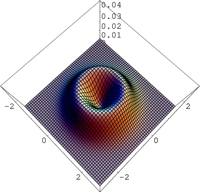
Figure 7: $x^{1}=x^{3}=0$ slice of the Wick symbol of $\left(\frac{\zeta}{4}\right)^{2}\frac{1}{16}F_{\mu\nu}F^{\mu\nu}$. Observe that it vanishes at the origin of ${\bf{R}}^{4}$.

Thus when represented in the Wick symbols, MvN gauge transformation induces topology change: It extracts a point from ${\bf{R}}^{4}$. However this is only a matter of representation in operator symbols and at the operator level nothing essentially changes because it is mere a change of the name. However the topological features of gauge field configuration is described only by using the operator symbols, and when represented in the Wick symbol, MvN gauge transformation gives a unified description for the topology change and gauge transformation. This mixing of gauge field and geometry is one of the most intriguing nature of the gauge theory on noncommutative space. From the IIB matrix model points of view, gauge field and geometry are indistinguishable: In (4.9) we regard $i\hat{\partial}_{\mu}$ as background and $iA_{\mu}$ as fluctuation, but the original variable in the IIB matrix model is $X_{\mu}$.

Calculation of $\left(\frac{\zeta}{4}\right)^{2}\frac{1}{16}F_{\mu\nu}^{(p_{\cal I})}F^{{(p_{\cal I})}\mu\nu}$ of $U(1)$ One-Instanton Solution

The field strength in ${\cal H}_{\cal I}$ can be calculated from (4.48):

$$F_{z_{1}\bar{z}_{1}}^{(p_{\cal I})}=-F_{z_{2}\bar{z}_{2}}^{(p_{\cal I})} = \frac{\zeta}{\left(\frac{\zeta}{2}\right)^{3}\hat{N}(\hat{N}+1)(\hat{N}+2)}\,(z_{1}\bar{z}_{1}-z_{2}\bar{z}_{2}),$$

$$F_{z_{1}\bar{z}_{2}}^{(p_{\cal I})}=F_{z_{2}\bar{z}_{1}}^{{(p_{\cal I})}\dagger} = \frac{\zeta}{\left(\frac{\zeta}{2}\right)^{3}\hat{N}(\hat{N}+1)(\hat{N}+2)}\,2z_{2}\bar{z}_{1},$$ (4.67)

where $\frac{\zeta}{2}\hat{N}=z_{1}\bar{z}_{1}+z_{2}\bar{z}_{2}$. The instanton number is given by

$$-\frac{1}{16\pi^{2}}\left(2\pi\frac{\zeta}{4}\right)^{2}\mbox{Tr}_{\cal H}F_{\mu\nu}^{(p_{\cal I})}\tilde{F}^{(p_{\cal I})\mu\nu}.$$ (4.68)

From (C) and (C.5), $\frac{1}{16}F_{\mu\nu}^{(p_{\cal I})}\tilde{F}^{(p_{\cal I})\mu\nu}=F_{z_{1}\bar{z}_{1}}^{(p_{\cal I})}F_{z_{2}\bar{z}_{2}}^{(p_{\cal I})}-\frac{1}{2}\left(F_{z_{1}\bar{z}_{2}}^{(p_{\cal I})}F_{z_{2}\bar{z}_{1}}^{(p_{\cal I})}+F_{z_{2}\bar{z}_{1}}^{(p_{\cal I})}F_{z_{1}\bar{z}_{2}}^{(p_{\cal I})}\right)$ and (4.68) becomes

(4.68) (4.69)

$$= -\frac{1}{\pi^{2}}\left(2\pi\frac{\zeta}{4}\right)^{2}\mbox{Tr}_{\cal H}\left(F_{z_{1}\bar{z}_{1}}^{(p_{\cal I})}F_{z_{2}\bar{z}_{2}}^{(p_{\cal I})}-\frac{1}{2}\left(F_{z_{1}\bar{z}_{2}}^{(p_{\cal I})}F_{z_{2}\bar{z}_{1}}^{(p_{\cal I})}+F_{z_{2}\bar{z}_{1}}^{(p_{\cal I})}F_{z_{1}\bar{z}_{2}}^{(p_{\cal I})}\right)\right)$$

$$= \frac{1}{\pi^{2}}\left(2\pi\frac{\zeta}{4}\right)^{2}\mbox{Tr}_{\cal H}\left(\frac{\zeta}{\left(\frac{\zeta}{2}\right)^{3}\hat{N}(\hat{N}+1)(\hat{N}+2)}\right)^{2}\left\{(z_{1}\bar{z}_{1}-z_{2}\bar{z}_{2})^{2}+2z_{2}\bar{z}_{1}z_{1}\bar{z}_{2}+2z_{2}\bar{z}_{1}z_{1}\bar{z}_{2}\right\}$$

$$= -\frac{1}{\pi^{2}}\left(2\pi\frac{\zeta}{4}\right)^{2}\mbox{Tr}_{\cal H}\,\,\zeta^{2}\left(\frac{\zeta}{2}\right)^{(-6+2)}\frac{1}{\hat{N}^{2}(\hat{N}+1)^{2}(\hat{N}+2)^{2}}(\hat{N}^{2}+2\hat{N})$$

$$= 4\sum_{(n_{1},n_{2})\neq(0,0)}\frac{1}{N(N+1)^{2}(N+2)}$$

$$= 4\sum_{N=1}^{\infty}\frac{1}{N(N+1)(N+2)}$$

$$= 1.$$

Thus we have checked again that the instanton number is one. The Wick symbol of $\left(\frac{\zeta}{4}\right)^{2}\frac{1}{16}F_{\mu\nu}^{(p_{\cal I})}F^{(p_{\cal I})\mu\nu}$ is given by

$$\Omega_{N}\left(\left(\frac{\zeta}{4}\right)^{2}\frac{1}{16}F_{\mu\nu}^{(p_{\cal I})}F^{(p_{\cal I})\mu\nu}\right)$$ (4.70)

$$= \sum_{(n_{1},n_{2})\neq(0,0)}\frac{1}{(n_{1}+n_{2})(n_{1}+n_{2}+1)^{2}(n_{1}+n_{2}+2)}\frac{r_{1}^{2n_{1}}}{n_{1}!}\frac{r_{2}^{2n_{2}}}{n_{2}!}e^{-r_{1}^{2}-r_{2}^{2}}.$$

where $r_{1}^{2}=\frac{2}{\zeta}((x^{1})^{2}+(x^{2})^{2})$ and $r_{2}^{2}=\frac{2}{\zeta}((x^{3})^{2}+(x^{4})^{2})$. We can rewrite (4.70) as follows:

$$\sum_{(n_{1},n_{2})\neq(0,0)}\!\!\!\!\!\! \!\!\!\!\!\!\frac{1}{(n_{1}+n_{2})(n_{1}+n_{2}+1)^{2}(n_{1}+n_{2}+2)}\,\,\frac{r_{1}^{2n_{1}}}{n_{1}!}\,\frac{r_{2}^{2n_{2}}}{n_{2}!}\,e^{-r_{1}^{2}-r_{2}^{2}}$$ (4.71)

$$= \sum_{N=1}^{\infty}\frac{1}{N(N+1)^{2}(N+2)}\sum_{n_{1}=0}^{N}\frac{1}{N!}\,\frac{N!}{n_{1}!\,(N-n_{1}!)}\,r_{1}^{2n_{1}}r_{2}^{2(N-n_{1})}e^{-r_{1}^{2}-r_{2}^{2}}$$

$$= \sum_{N=1}^{\infty}\frac{1}{N(N+1)^{2}(N+2)}\,\frac{r^{2N}}{N!}\,e^{-r^{2}},\qquad r^{2}=r_{1}^{2}+r_{2}^{2}\,\,.$$

5 Summary and Future Directions

Summary

In the lectures I have clarified the topological origin of the instanton number of $U(1)$ gauge field on noncommutative ${\bf{R}}^{4}$. The mechanism that gives instanton number is quite impressive: the projection operator reduces the instanton number to the winding number of gauge field around $S^{1}$ at infinity. I would like to emphasise again that using operator symbols, every topological nature of the noncommutative instantons can be described clearly. The existence of non-singular $U(1)$ instantons is due to the intriguing nature of the noncommutativity, but it is not mysterious.

Noncommutative $U(1)$ instanton solutions with instanton number $k$ has one-to-one correspondence with the codimension $k$ ideal and we can consider the projection to the ideal states. In order to clarify the physical meaning of these projection operators, I introduced the notion of the gauge theory on restricted subspace of the Fock space ${\cal H}$. Generalized gauge equivalence relation follows from partial isometry between two infinite dimensional subspaces of the Fock space. Two projections related by partial isometry is called Murray-von Neumann equivalent. We determined transformation rule of gauge field under partial isometry map, and call it Murray-von Neumann (MvN) gauge transformation. This formalism is not the noncommutative Yang-Mills theory in the usual sense, but it is a natural extension. Indeed, MvN gauge transformation contains the noncommutative counterparts of the singular gauge transformation in commutative space. From the IIB matrix model viewpoints partial isometry is mere a change of names of states in the Fock space, and should not change physics. By using this formalism the instanton number is explained as dimension of projection which characterizes instanton solution. This is an algebraic description of the instanton number, and the MvN gauge transformation relates the algebraic description of the instanton number to the topological one.

In the Wick symbol representation, the MvN gauge transformation induces a noncommutative analog of topology change. At first sight the equivalence relation among spaces with different topology is terrifying, but at the operator level nothing essentially changes under the MvN gauge transformation. This unified description of gauge field and geometry is one of the most intriguing features of the gauge theory on noncommutative space, and fits very naturally to the framework of the IIB matrix model.

Indication to the Ordinary Gauge Theory Description

In [6] it was conjectured that there is a one-to-one map between ordinary description and noncommutative description. Motivated by this conjecture some solutions of ordinary $U(1)$ gauge theory were constructed [6][12][13][14]. However non of these solutions have asymptotic behaviour of noncommutative $U(1)$ instanton discussed in section 3.3. Therefore if there exists such map between ordinary and noncommutative descriptions, these solutions must (at least approximately) correspond to the gauge field restricted in ${\cal H}_{\cal I}$ discussed in section 4.2. In this case there is a projection at the core of instanton, and the covariant derivative is appropriately modified. This modification of the covariant derivative can be interpreted as topology change noncommutative space. This suggests that in corresponding ordinary description, if it exists, there must be a topology change from ${\bf{R}}^{4}$. Furthermore, the existence of MvN gauge transformation in noncommutative space suggests that this topology change in ordinary description is (some kind of) gauge dependent notion, and there is a explanation without topology change. In [14], it was conjectured that ordinary description requires a modification of base space topology, which has some similarities with the gauge theory in restricted Fock space. If one seriously try to establish explicit relation between ordinary and noncommutative descriptions in the case of instantons, the discussions in the lecture notes must be taken into account. I would like to mention that in the case of monopoles and BIons, there are little bit clearer descriptions for the change of geometry in ordinary descriptions [15][16][17][18][19][20].

D-brane Charge and Noncommutative Geometry

In string theory, instantons describe the bound states of D$p$-branes and D$(p+4)$-branes [21][22]. In this regard the relation between projection operator and D-brane charge was first pointed out in [3], and the relations between projection operator, partial isometry and the topological charge in noncommutative gauge theory was first clarified in [4]. In the case of branes in the closed string vacuum, K-theoretical classification of D-brane charge [23][24] in certain NS-NS B-field background was recently investigated in [26][27][28][29] extending the techniques introduced in [30].

Surface Term and Trace

In mathematical definition, trace must satisfy the following “trace property”

$$\mbox{Tr}AB=\mbox{Tr}BA.$$ (5.1)

Here $A$ and $B$ are elements of some algebra and Tr is a trace of that algebra. However in the lecture notes, we have encounter the quantity like

$$\mbox{Tr}_{{\cal H}}[\hat{\partial}_{\mu},K^{\mu}]\neq 0.$$ (5.2)

This means the trace $\mbox{Tr}_{{\cal H}}$ and unbounded operator $\hat{\partial}_{\mu}$ do not satisfy trace property (5.1). However, as we have seen, such quantity is important because it gives topological charges. Thus in order to obtain physically interesting results, we should consider about loosening the requirement (5.1). In [25] noncommutative geometric formulation of string field theory was proposed. In recent progress in string theory it is becoming very plausible that the R-R charge of D-branes is classified in the stringy algebra [26][31]. In this case if we loosen the requirement (5.1) and D-brane will be represented by some unbounded operator which gives surface terms. In string field theory the trace property (5.1) is proved under certain conditions, but it may be useful to carefully re-examine these conditions. The deep meaning of the tachyon condensation conjecture [32] will be clarified by establishing the topological/algebraic description of the tachyon potential in string field theory. The techniques developed here may help the analysis of topological as well as algebraic classification of D-brane R-R charges.

Acknowledgements

The contents of the lecture notes based on talks given at APCTP-Yonsei Summer Workshop on Noncommutative Field Theories, Tokyo University (Hongo) and Tokyo Institute of Technology. I thank the audiences for questions and comments. I also thank participants of the workshop for many interesting discussions, especially I am grateful to S. Terashima for explanations and discussions. I would also like to thank organizers of the workshop for warm hospitality.

Appendix A The Case of $U(2)$ Instanton

In this section we construct $U(2)$ one-instanton solution and observe the difference from the $U(1)$ solution. In this section we set $\zeta=2$ for simplicity. A solution to the ADHM equation (3.18) is given by

$$B_{1}=B_{2}=0,\quad I=(\sqrt{\rho^{2}+2}\,\,\,\,0\,),\,\,J^{\dagger}=(\,0\,\,\,\rho\,).$$ (A.1)

Then the operator ${\cal D}_{z}$ becomes

$${\cal D}_{z}=\left(\begin{array}[]{cccc}-z_{2}&-z_{1}&\sqrt{\rho^{2}+2}&0\\ \bar{z}_{1}&-\bar{z}_{2}&0&\rho\end{array}\right).$$ (A.4)

The operator zero-mode can be obtained as

$$\Psi_{0}=\left(\begin{array}[]{cc}&\\ \Psi^{(1)}_{0}&\Psi^{(2)}_{0}\\ &\end{array}\right)\,,\, \Psi^{(1)}_{0}=\left(\begin{array}[]{c}\sqrt{\rho^{2}+2}\,\bar{z}_{2}\\ \sqrt{\rho^{2}+2}\,\bar{z}_{1}\\ z_{1}\bar{z}_{1}+z_{2}\bar{z}_{2}\\ 0\end{array}\right)\frac{1}{\sqrt{\hat{N}(\hat{N}+2+\rho^{2})}},$$ (A.17)

$$\Psi^{(2)}_{0}=\left(\begin{array}[]{c}-\rho z_{1}\\ \rho z_{2}\\ 0\\ z_{1}\bar{z}_{1}+z_{2}\bar{z}_{2}+2\end{array}\right)\frac{1}{\sqrt{(\hat{N}+2)(\hat{N}+2+\rho^{2})}},$$

where $\frac{1}{\sqrt{\hat{N}}}$ is defined as

$$\frac{1}{\sqrt{\hat{N}}}=\sum_{(n_{1},n_{2})\neq(0,0)}\frac{1}{\sqrt{n_{1}+n_{2}}}\,|n_{1},n_{2}\rangle\langle n_{1},n_{2}|,$$ (A.19)

i.e. when we consider the inverse of $\sqrt{\hat{N}}$ we omit the kernel of $\sqrt{\hat{N}}$, that is, $|0,0\rangle$, from the Fock space. Hence $\frac{1}{\sqrt{\hat{N}}}$ is a well defined operator. When $\rho=0$, the contribution of $\Psi_{0}^{(2)}$ to the field strength vanishes whereas $\Psi_{0}^{(1)}$ reduces to the operator zero-mode (3.74) in $U(1)$ one-instanton solution. This operator zero-mode $\Psi_{0}$ is normalized as

$$\Psi^{\dagger}_{0}\Psi_{0}=p,$$ (A.20)

where $p$ is a projection in the algebra of $2\times 2$ operator valued matrices:

$$p=\left(\begin{array}[]{cc}\mbox{Id}_{\cal H}-|0,0\rangle\langle 0,0|&0\\ 0&\mbox{Id}_{\cal H}\end{array}\right).$$ (A.23)

Although in the case where the gauge group is $U(2)$ the vector zero-modes have not been classified at the moment, we can directly check that the equation

$${\cal D}_{z}^{\dagger}\frac{1}{{\cal D}_{z}{\cal D}_{z}^{\dagger}}{\cal D}_{z}=1-\Psi_{0}\Psi^{\dagger}_{0},$$ (A.24)

holds. Therefore the covariant derivative operator

$$\hat{D}_{\mu}^{(p)} = p\hat{\partial}_{\mu}p+A_{\mu}^{(p)},$$ (A.25)

$$A_{\mu}^{(p)}=\Psi_{0}^{\dagger}(\partial_{\mu}\Psi_{0})p,$$

gives anti-self-dual field strength.

Since the projection $p$ has infinite rank as an operator, it is Murray-von Neumann equivalent to the identity operator $\mbox{Id}_{{\cal H}}\otimes\mbox{Id}_{2}$. So let us MvN gauge transform $p$ to $\mbox{Id}_{{\cal H}}\otimes\mbox{Id}_{2}$. In order to do so one seeks for the operator $U$ which satisfies

$$U^{\dagger}U=p,\quad UU^{\dagger}=\mbox{Id}_{{\cal H}}\otimes\mbox{Id}_{2}.$$ (A.26)

Of course there are (infinitely) many gauge equivalent choices for such $U$. In the case where the gauge group is $U(2)$, there is a choice which has a physically interesting interpretation. Let us consider following operator $U$ which satisfies (A.26) [4]:

$$U^{\dagger}=\left(\begin{array}[]{cc}z_{2}\frac{1}{\sqrt{\hat{N}+1}}&z_{1}\frac{1}{\sqrt{\hat{N}+1}}\\ -\bar{z}_{1}\frac{1}{\sqrt{\hat{N}+1}}&\bar{z}_{2}\frac{1}{\sqrt{\hat{N}+1}}\end{array}\right).$$ (A.29)

In large $r$ limit the Wick symbol of this operator becomes

$$U^{\dagger}\rightarrow g^{\dagger}\equiv\frac{1}{r}\left(\begin{array}[]{cc}z_{2}&z_{1}\\ -\bar{z}_{1}&\bar{z}_{2}\end{array}\right)\qquad(r\rightarrow\infty).$$ (A.32)

The asymptotic form of the gauge field $A_{\mu}=(U\Psi_{0}^{\dagger})\partial_{\mu}(\Psi_{0}U)$ becomes

$$A_{\mu}\rightarrow g\partial_{\mu}g^{\dagger}\quad(r\rightarrow\infty).$$ (A.33)

Thus in the case of $U(2)$ gauge theory we can understand the topological origin of the instanton number in the same way as in the ordinary case. Note that (A.29) is a noncommutative analog of the singular gauge transformation (see for example [4][34]), which is smoothened by the noncommutativity.

Appendix B $U(1)$ Instantons on Noncommutative ${\bf{R}}^{4}$, Ideal and Projections

B.1 Ideal

Suppose we are given a ring $R$. A subset ${\cal I}\in R$ is called ideal if it satisfies following two conditions:

$$a,b\in{\cal I}\Longrightarrow a+b={\cal I},$$ (B.1)

$$\forall r\in R,a\in{\cal I},\,\,r\cdot a\in{\cal I}.$$ (B.2)

This definition of ideal is taken from the property of the kernel of map. As an example, let us consider the ring of polynomials of complex number $z$ which we denote by ${\cal O}_{z}$. Let us consider the subset $(z-w){\cal O}_{z}$ which consists of all the polynomials of the form $(z-w)f(z)$. This subset is ideal since

$$(z-w)f(z)+(z-w)g(z) = (z-w)(f(z)+g(z)),$$

$$r(z)\cdot(z-w)f(z) = (z-w)(r(z)f(z)).$$ (B.3)

$$\qquad f(z),g(z),r(z)\in{\cal O}_{z}.$$

This ideal is called “ ideal generated by $z-w$”. Let us consider the map $\phi_{w}$ from polynomials to complex number ${\cal O}_{z}\mapsto\bf{C}$ by $\phi_{w}(f(z))=f(w)$. Then $\ker\phi_{w}=(z-w){\cal O}_{z}$, that is, the ideal generated by $z-w$.

B.2 One-To-One Correspondence Between
$U(1)$ Instantons on Noncommutative ${\bf{R}}^{4}$ and Ideal

In this subsection we review part of the beautiful works of Nakajima [36][37], which is relevant to our discussions: We explain one-to-one correspondence between $U(1)$ $k$-instanton solution on noncommutative ${\bf{R}}^{4}$ and ideal ${\cal I}\subset{\cal O}_{{\bf{C}}^{2}}$ with $\mbox{dim}_{{\bf{C}}}\,{\cal O}_{{\bf{C}}^{2}}/{\cal I}=k$. First we show the isomorphism

$$\ker{\cal D}_{z}\simeq{\cal I}=\left\{f(z_{1},z_{2})\Bigm{|}f(B_{1},B_{2})=0\right\}.$$ (B.4)

This isomorphism gives a map from the noncommutative $U(1)$ instantons and to the projections to the space of ideal states $p_{\cal I}$.

Let us consider the space of vector zero-modes of ${\cal D}_{z}$, $\ker{\cal D}_{z}=\ker\tau_{z}\cap\ker\sigma^{\dagger}_{z}$:

$$\left|V\right\rangle=\left(\begin{array}[]{c}\left|u_{1}\right\rangle\\ \left|u_{2}\right\rangle\\ \left|\,f\,\right\rangle\end{array}\right)\quad\in\ker\tau_{z}\cap\ker\sigma^{\dagger}_{z}\quad.$$ (B.8)

The projection to third factor

$$\left|V\right\rangle=\left(\begin{array}[]{c}\left|u_{1}\right\rangle\\ \left|u_{2}\right\rangle\\ \left|\,f\,\right\rangle\end{array}\right)\hookrightarrow\,\left|\,f\,\right\rangle=f(z_{1},z_{2})\left|\,0,0\,\right\rangle,$$ (B.12)

gives the inclusion

$$\ker\tau_{z}\cap\ker\sigma^{\dagger}_{z}\hookrightarrow{\cal H}.$$ (B.13)

We denote its image by ${\cal H}_{\cal I}$. It is easy to see that for $f(z)\left|\,0,0\,\right\rangle\in{\cal H}_{\cal I}$,

$$f(z)\left|\,0,0\,\right\rangle\in{\cal I}$$ (B.14)

$$\Leftrightarrow {}^{\exists}u_{1}(z)\left|\,0,0\,\right\rangle,u_{2}(z)\left|\,0,0\,\right\rangle,\in{\cal H}\otimes{\bf{C}}^{k}$$

$$\mbox{such that}\quad f(z)\left|\,0,0\,\right\rangle I=(B_{2}-z_{2})u_{1}(z)\left|\,0,0\,\right\rangle+(B_{1}-z_{1})u_{2}(z)\left|\,0,0\,\right\rangle$$

$$\Leftrightarrow f(B_{1},B_{2})I=0.$$

Since the vectors of the form $B_{1}^{p}B_{2}^{q}I,\,\,p,q\in{\bf Z}_{\geq 0}$ span the whole $V={\bf C}^{k}$ by the stability discussed later in this appendix, it follows that $f(z)\left|\,0,0\,\right\rangle\in{\cal H}_{\cal I}$ implies $f(B_{1},B_{2})=0$.

Conversely, suppose $f(B_{1},B_{2})=0$. Then,

$$f(z_{1},z_{2})\mbox{Id}_{V}=f(z_{1}-B_{1}+B_{1},z_{2}-B_{2}+B_{2})$$ (B.15)

$$= f(B_{1},B_{2})+(z_{2}-B_{2})(C(z)+(z_{1}-B_{1})E(z))+(z_{1}-B_{1})(D(z)-(z_{2}-B_{2})E(z))$$

$$= (z_{2}-B_{2})(C(z)+(z_{1}-B_{1})E(z))+(z_{1}-B_{1})(D(z)-(z_{2}-B_{2})E(z)).$$

for some $C(z),D(z)$ and arbitrary $E(z)$ where $C(z),D(z)$ and $E(z)$ are $k\times k$ matrices whose entries are polynomials in $z_{1}$ and $z_{2}$. We fix the ambiguity in $E(z)$ by requiring

$$(\bar{z}_{1}-B^{\dagger}_{1})C(z)-(\bar{z}_{2}-B^{\dagger}_{2})D(z)=0.$$ (B.16)

This condition completely eliminates ambiguity since

$$(\bar{z}_{1}-B^{\dagger}_{1})\tilde{C}(z)-(\bar{z}_{2}-B^{\dagger}_{2})\tilde{D}(z)=0$$ (B.17)

$$\mbox{for}\,\,\tilde{C}(z)=C(z)+(z_{1}-B_{1})E(z),\,\tilde{D}(z)=D(z)-(z_{2}-B_{2})E(z)$$

$$\Leftrightarrow (\bar{z}_{1}-B^{\dagger}_{1})(z_{1}-B_{1})E(z)+(\bar{z}_{2}-B^{\dagger}_{2})(z_{2}-B_{2})E(z)=0$$

$$\Leftrightarrow (E(z))^{\dagger}(\bar{z}_{1}-B^{\dagger}_{1})(z_{1}-B_{1})E(z)+(E(z))^{\dagger}(\bar{z}_{2}-B^{\dagger}_{2})(z_{2}-B_{2})E(z)=0$$

$$\Leftrightarrow (z_{1}-B_{1})E(z)=(z_{2}-B_{2})E(z)=0$$

$$\Leftrightarrow \tilde{C}(z)=C(z),\quad\tilde{D}(z)=D(z).$$

If we write $u_{1}(z)=C(z)I,u_{2}(z)=D(z)I$, we obtain

$$f(z)I\left|\,0,0\,\right\rangle=-(B_{2}-z_{2})u_{1}(z)\left|\,0,0\,\right\rangle-(B_{1}-z_{1})u_{2}(z)\left|\,0,0\,\right\rangle,$$ (B.18)

with

$$(B_{1}^{\dagger}-\bar{z_{1}})u_{1}(z)\left|\,0,0\,\right\rangle-(B_{2}^{\dagger}-\bar{z_{2}})u_{2}(z)\left|\,0,0\,\right\rangle=0.$$ (B.19)

Therefore $f(z)\left|\,0,0\,\right\rangle\in{\cal H}_{\cal I}$. This completes the proof of (B.4).

Stability

The positivity of $\zeta$ ensures the following stability [36][11] for any solution of ADHM equation (3.18):

$$\bullet S V={\bf C}^{k} B_{a}(S)\subset S\,(a=1,2)$$ Any subspace of which satisfies (B.20)

and Im $$I\,\subset S V$$ is equal to .

Proof
Suppose (B.20) does not hold. Then there exists subspace $S(\neq\emptyset)$ of $V$ such that $B_{a}(S)\subset S$ and Im $I\,\subset S$. Let $S_{\bot}$ be the subspace of $V$ orthogonal to $S$. Then $B_{a}$ and $B_{a}^{\dagger}$ acquire the form

$$B_{a}=\left(\begin{array}[]{cc}B_{a}|_{S}&D_{a}\\ 0&(B_{a}^{\dagger}|_{S_{\bot}})^{\dagger}\end{array}\right)\quad\left(B_{a}^{\dagger}=\left(\begin{array}[]{cc}(B_{a}|_{S})^{\dagger}&0\\ D_{a}^{\dagger}&B_{a}^{\dagger}|_{S_{\bot}}\end{array}\right)\right)$$ (B.21)

Notice that the action of $B_{a}$ and $B_{a}^{\dagger}$ are closed respectively on $S$ and $S_{\bot}$. $B_{a}|_{S}$ and $B_{a}^{\dagger}|_{S_{\bot}}$ are their restrictions on $S$ and $S_{\bot}$. The restriction of the real ADHM equation (3.18) to the subspace $S_{\bot}$ can be written as

$$\sum_{a}[(B_{a}^{\dagger}|_{S_{\bot}})^{\dagger},B_{a}^{\dagger}|_{S_{\bot}}]-\sum_{a}D_{a}^{\dagger}D_{a}-J|_{S_{\bot}}(J|_{S_{\bot}})^{\dagger}=\zeta|_{S_{\bot}}$$ (B.22)

where $J|_{S_{\bot}}$ is a projection of $J$ onto $S_{\bot}$. Taking the trace of this equation leads to a contradiction because we set $\zeta>0$. Therefore $S=\emptyset$.

From the stability condition (B.20) we can deduce dim ${\cal H}_{/{\cal I}}=k$. We define a map $\phi$: ${\cal H}\mapsto{\bf{C}}^{k}$ by $\phi\left(f(z_{1},z_{2})\left|0,0\right\rangle\right)=f(B_{1},B_{2})I$. Since $B_{\alpha}(\mbox{Im}\,\phi)\subset\mbox{Im}\,\phi$ ($\alpha=1,2$) and $\mbox{Im}\,\phi$ contains $I$, it must be ${\bf{C}}^{k}$ from the stability condition. Hence $\phi$ is surjective. We define ${\cal I}\equiv\ker\phi$. Then ${\cal I}$ is an ideal in ${\cal H}$ and $\mbox{dim}\,{\cal H}_{/{\cal I}}=\mbox{dim}\,({\cal H}/{\cal H}_{\cal I})=k$.

Thus we have shown that every noncommutative $U(1)$ instanton has corresponding ideal ${\cal I}\subset{\cal O}_{{\bf{C}}^{2}}$ with $\mbox{dim}_{{\bf{C}}}\,{\cal O}_{{\bf{C}}^{2}}/{\cal I}=k$. The inverse is also true: Every codimension $k$ ideal ${\cal I}$ has corresponding noncommutative $U(1)$ instanton with instanton number $k$. To show this, we consider the moduli space of $U(1)$ instantons on noncommutative ${\bf{R}}^{4}$. Recall that we can construct instantons from the solution of the ADHM equation (3.18):

$$\mu_{\bf{R}} \equiv [B_{1},B_{1}^{\dagger}]+[B_{2},B_{2}^{\dagger}]+II^{\dagger}-J^{\dagger}J=\zeta\mbox{Id}_{k},$$ (B.23)

$$\mu_{\bf C} \equiv [B_{1},B_{2}]+IJ=0.$$ (B.24)

There is an action of $U(k)$ that does not change the gauge field constructed by ADHM method:

$$(B_{1},B_{2},I,J)\mapsto(uB_{1}u^{-1},uB_{2}u^{-1},uI,Ju^{-1}),\qquad u\in U(k).$$ (B.25)

Therefore the moduli space of $U(1)$ instantons on noncommutative ${\bf{R}}^{4}$ with instanton number $k$ is given by

$${\cal M}_{\zeta}(k,n=1)=\mu^{-1}_{\bf{R}}(\zeta)\cap\mu^{-1}_{\bf{C}}(0)/U(k),$$ (B.26)

where the action of $U(k)$ is the one given in (B.25). This moduli space is equivalently described as follows [37]:

$${\cal M}_{\zeta}(k,n=1)\simeq\mu^{-1(s)}_{\bf{C}}(0)/GL(k),$$ (B.27)

where

$$\mu^{-1(s)}_{\bf{C}}(0)\equiv\Biggl{\{}(B_{\alpha},I,J)\Biggr{|}\begin{array}[]{l}(1)\,\mu_{\bf{C}}=0\\ (2)\,\mbox{stability condition}\,(\ref{stability})\end{array}\Biggl{.}\Biggr{\}}.$$ (B.30)

The proof is given in [37]. Then we have the following isomorphism

$${\cal M}_{\zeta}(k,n=1)\simeq({\bf{C}}^{2})^{[k]}\equiv\Biggl{\{}{\cal I}\subset{\cal O}_{{\bf{C}}^{2}}\Biggr{|}\begin{array}[]{l}{\cal I}\,\mbox{is an ideal}\\ \mbox{dim}\,{\cal O}_{{\bf{C}}^{2}}/{\cal I}=k\end{array}\Biggl{.}\Biggr{\}}.$$ (B.33)

Suppose we have have an ideal ${\cal I}\in({\bf{C}}^{2})^{[k]}$. Then we can construct a projection to the ideal states $p_{\cal I}$. Then we define ${\cal H}_{\cal I}\equiv p_{\cal I}{\cal H}$, ${\cal H}_{/{\cal I}}\equiv(1-p_{\cal I}){\cal H}$ , and define $B_{\alpha}\in\mbox{End}{\cal H}_{/{\cal I}}$ as the multiplication by $z_{\alpha}$ mod ${\cal H}_{\cal I}$ for $\alpha=1,2$ and define $I\equiv\left|0,0\right\rangle$ mod ${\cal H}_{\cal I}$. It follows $[B_{1},B_{2}]=0$. Since when $n=1$, one can show $J=0$ from $(1)$ and $(2)$ [37], this condition is equivalent to $\mu_{\bf{C}}=0$. The stability condition holds since $\left|0,0\right\rangle$ multiplied by $z_{\alpha}$ span whole ${\cal H}$. $GL(k)$ in (B.27) corresponds to the change of basis (not orthonormal) in ${\cal H}_{/{\cal I}}$.

Appendix C Convention for the Complex Coordinates

Complex coordinates:

$$z_{1}=x^{2}+ix^{1},\quad z_{2}=x^{4}+ix^{3}.$$ (C.1)

Field strength:

$$F_{z_{i}\bar{z}_{j}}\equiv[D_{z_{i}},D_{\bar{z}_{j}}],\quad F_{z_{i}z_{j}}\equiv[D_{z_{i}},D_{z_{j}}],\quad(i,j=1,2)$$ (C.2)

where

$$D_{z_{1}}=\frac{1}{2}(D_{2}-iD_{1}),\quad D_{z_{2}}=\frac{1}{2}(D_{4}-iD_{3}),$$

$$D_{\bar{z}_{1}}=\frac{1}{2}(D_{2}+iD_{1}),\quad D_{\bar{z}_{2}}=\frac{1}{2}(D_{4}+iD_{3}).$$ (C.3)

Here $D_{\mu}=\partial_{\mu}+A_{\mu}$. Then we obtain

$$F_{z_{1}\bar{z}_{1}}=\frac{1}{4}[(D_{2}-iD_{1}),(D_{2}+iD_{1})]=-\frac{i}{2}F_{12},$$

$$F_{z_{2}\bar{z}_{2}}=\frac{1}{4}[(D_{4}-iD_{3}),(D_{4}+iD_{3})]=-\frac{i}{2}F_{34},$$ (C.4)

$$F_{z_{1}z_{2}}=\frac{1}{4}[(D_{2}-iD_{1}),(D_{4}-iD_{3})]=\frac{1}{4}\left(F_{24}-F_{13}-i(F_{23}+F_{14})\right),$$

$$F_{z_{1}\bar{z}_{2}}=\frac{1}{4}[(D_{2}-iD_{1}),(D_{4}+iD_{3})]=\frac{1}{4}\left(F_{24}+F_{13}+i(F_{23}-F_{14})\right).$$ (C.5)

The anti-self-dual conditions:

$$F_{z_{1}\bar{z}_{1}}+F_{z_{2}\bar{z}_{2}}=0 \Leftrightarrow F_{12}+F_{34}=0,$$ (C.6)

$$F_{z_{1}z_{2}}=0 \Leftrightarrow \left\{\begin{array}[]{r}F_{13}-F_{24}=0,\\ F_{14}+F_{23}=0.\end{array}\right.$$ (C.9)

Appendix D Some Formulas in Operator Calculus

• Projection operators:

  $$p^{2}=p,\,\,p^{\dagger}=p,$$

  $$p(1-p)=(1-p)p=0.$$ (D.1)

  Since for operators $A,B$ and $C$,

  $$[A,BC]=[A,B]C+B[A,C],$$

  $$[AB,C]=[A,C]B+A[B,C],$$ (D.2)

  we obtain following equations:

  $$p[\hat{\partial}_{\mu},p] = -p[\hat{\partial}_{\mu},1-p]=-[\hat{\partial}_{\mu},p(1-p)]+[\hat{\partial}_{\mu},p](1-p)$$

  $$= [\hat{\partial}_{\mu},p](1-p),$$

  $$\quad[\hat{\partial}_{\mu},p]p, = (1-p)[\hat{\partial}_{\mu},p]$$

  $$p[\hat{\partial}_{\mu},p]p = 0.$$ (D.3)

• Similarity transformation:

  $$e^{A}\,B\,e^{-A}=B+[A,B]+\frac{1}{2!}[A,[A,B]]+\cdots=\left[\sum_{n=0}^{\infty}\frac{1}{n!}{\it\Delta}_{A}^{n}\right]\,B,$$ (D.4)

  where ${\it\Delta}_{A}B:=[A,B]$.
  

• When $[A,B]$ commutes with both $A$ and $B$,

  $$e^{A}\,e^{B} = e^{[A,B]}\,e^{B}\,e^{A}\quad.$$

  $$e^{A}\,e^{B} = e^{\frac{1}{2}[A,B]}e^{A+B}\quad.$$ (D.5)

References

• [1] A. Connes, M. R. Douglas and A. Schwarz, “Noncommutative Geometry and Matrix Theory: Compactification on Tori”, JHEP 9802 (1998) 003.
• [2] N. Nekrasov and A. Schwarz, “Instantons on Noncommutative ${\bf R}^{4}$ and $(2,0)$ Superconformal Six Dimensional Theory”, Comm. Math. Phys. 198 (1998) 689.
• [3] K. Furuuchi, “Instantons on Noncommutative ${\bf R}^{4}$ and Projection Operators”, Prog. Theor. Phys. 103 (2000) 1043, hep-th/9912047.
• [4] K. Furuuchi, “Equivalence of Projections as Gauge Equivalence on Noncommutative Space”, hep-th/0005199.
• [5] O. Aharony, M. Berkooz and N. Seiberg, “Light-Cone Description of (2,0) Superconformal Theories in Six Dimensions”, Adv. Theor. Math. Phys. 2 (1998) 119.
• [6] N. Seiberg and E. Witten, “String Theory and Noncommutative Geometry”, JHEP 9909 (1999) 032.
• [7] N. Ishibashi, H. Kawai, Y. Kitazawa, A. Tsuchiya, “A Large-N Reduced Model as Superstring”, Nucl. Phys. B498 (1997) 467.
• [8] H. Aoki, N. Ishibashi, S. Iso, H. Kawai, Y. Kitazawa, T. Tada “Noncommutative Yang-Mills in IIB Matrix Model”, Nucl. Phys. B565 (2000) 176.
• [9] P.-M. Ho, “Twisted Bundle on Noncommutative Space and $U(1)$ Instanton” hep-th/003012.
• [10] K. Furuuchi, H. Kunitomo and T. Nakatsu, “Topological Field Theory and Second-Quantized Five-Branes”, Nucl. Phys. B494 (1997) 144.
• [11] T. Nakatsu, “Toward Second-Quantization of D5-Brane”, Int. Jour. Mod. Phys. A13 (1998) 923.
• [12] M. Marino, R. Minasian, G. Moore, A. Strominger, “Nonlinear Instantons from Supersymmetric p-Branes”, JHEP 0001 (2000) 005.
• [13] S. Terashima, “Instantons in the $U(1)$ Born-Infeld Theory and Noncommutative Gauge Theory” Phys.Lett. B477 (2000) 292.
• [14] H. Braden and N. Nekrasov, “Space-Time Foam From Non-Commutative Instantons”, hep-th/9912019.
• [15] K. Hashimoto, “Born-Infeld Dynamics in Uniform Electric Field” JHEP 9907 (1999) 016.
• [16] A. Hashimoto and K. Hashimoto, “Monopoles and Dyons in Non-Commutative Geometry”, JHEP 9911 (1999) 005.
K. Hashimoto, H. Hata and S. Moriyama, “Brane configuration from monopole solution in non-commutative super Yang-Mills theory”, JHEP 9912, 021 (1999).
K. Hashimoto and T. Hirayama, “Branes and BPS configurations of noncommutative / commutative gauge theories”, hep-th/0002090.
• [17] D. Bak, “Deformed Nahm equation and a noncommutative BPS monopole”, Phys. Lett.  B471, 149 (1999).
• [18] D. Mateos, “Noncommutative vs. commutative descriptions of D-brane BIons”, Nucl. Phys. B577 (2000) 139.
• [19] S. Moriyama, “Noncommutative monopole from nonlinear monopole”, Phys. Lett.  B485, (2000) 278.
• [20] D. J. Gross and N. A. Nekrasov, “Monopoles and strings in noncommutative gauge theory”, JHEP 0007, 034 (2000).
D. J. Gross and N. A. Nekrasov, “Dynamics of strings in noncommutative gauge theory”, hep-th/0007204.
• [21] E. Witten, “Small Instantons in String Theory”, Nucl. Phys. B460 (1996) 541.
• [22] M. R. Douglas, “Branes within Branes”, hep-th/9512077.
• [23] R. Minasian and G. Moore, “K-theory and Ramond-Ramond charge” JHEP 9711 (1997) 002.
• [24] E. Witten, “D-Branes And K-Theory” JHEP 9812 (1998) 019.
• [25] E. Witten, “Non-commutative Geometry and String Theory” Nucl. Phys. B268 (1986) 253.
• [26] E. Witten, “ Noncommutative Tachyons And String Field Theory” hep-th/0006071.
• [27] J. Harvey, P. Kraus, F. Larsen, E. Martinec, “D-branes and Strings as Non-commutative Solitons” JHEP 0007 (2000) 042.
• [28] Y. Matsuo, “Topological Charges of Noncommutative Soliton” hep-th/0009002.
• [29] J. Harvey and G. Moore, “Noncommutative Tachyons and K-Theory” hep-th/0009030.
• [30] R. Gopakumar, S. Minwalla, A. Strominger, “Noncommutative Solitons” JHEP 0005 (2000) 020.
• [31] E. Witten, “Overview Of K-Theory Applied To Strings” hep-th/0007175.
• [32] A. Sen, “Tachyon Condensation on the Brane Antibrane System”, JHEP 9808 (1998) 012.
• [33] S. Coleman, “Uses of Instantons”, in Aspects of Symmetry Cambridge University Press (1985).
• [34] R. Rajaraman, “Solitons and Instantons”, North-Holland (1982).
• [35] M. Atiyah, N. Hitchin, V. Drinfeld and Y. Manin, “Construction of Instantons”, Phys. Lett. 65A (1978) 185.
E. Corrigan and P. Goddard, “Construction of instanton monopole solutions and reciprocity”, Ann. Phys. 154 (1984) 253.
S. Donaldson, “Instantons and Geometric Invariant Theory”, Comm. Math. Phys. 93 (1984) 453.
• [36] H. Nakajima, “Heisenberg algebra and Hilbert schemes of points on projective surfaces”, Ann. of Math. 145, (1997) 379, alg-geom/9507012.
H. Nakajima, “Instantons and affine Lie algebra”, Nucl. Phys. Proc. Suppl. 46 (1996) 154, alg-geom/9510003.
• [37] H. Nakajima, “Lectures on Hilbert scheme of points on surfaces”, AMS University Lecture Series vol. 18 (1999).
• [38] N.E. Wegge-Olsen, “K-Theory and $C^{*}$-Algebras”, Oxford University Press (1993).