STUDY OF THE O(N) LINEAR $\sigma$ MODEL AT FINITE TEMPERATURE USING THE 2PPI EXPANSION

Abstract

We show that a new expansion which sums seagull and bubble graphs to all orders, can be applied to the O(N)-linear $\sigma$-model at finite temperature. We prove that this expansion can be renormalised with the usual counterterms in a mass independent scheme and that Goldstone’s theorem is satisfied at each order. At the one loop order of this expansion, the Hartree result for the effective potential (daisy and superdaisy graphs) is recovered. We show that at one loop 2PPI order, the self energy of the $\sigma$-meson can be calculated exactly and that diagrams are summed beyond the Hartree approximation.

1 Introduction

In this paper, we will study the O(N) lineair $\sigma$-model at finite temperature, using the 2PPI expansion [1,2]. This model has always been a fertile ground to test ideas and check approximations in finite temperature quantum field theory [3] and has recently attracted renewed interest [4-11] because of its relevance to the thermodynamics of chiral symmetry in Q.C.D. Many treatments of finite T O(N) linear $\sigma$-model use the Hartree approximation which sums bubble graphs (daisy and superdaisy graphs). The standard way of summing these graphs is to use the 2PI expansion or CJT-method [12]. In this approach, only the 2PI diagrams are retained, which do not seperate in two pieces when two internal lines are cut. This sums self energy insertions but comes at the cost of introducing a self consistency condition which in general entails intractable non-local integral equations. When restricted to order $\lambda$, the 2PI expansion sums daisy and superdaisy graphs which alleviates some of the problems at finite T [4]. However, it is not feasible to extend this approach to higher order in $\lambda$ and therefore some of the basic problems of the O(N) linear $\sigma$-model at finite T are still unsolved. Another problem encountered is renormalizability. In [4], the daisy and superdaisy graphs are summed with the 2PI expansion at O$(\lambda)$, using bare perturbation theory. It is found that the effective bubble mass is finite when the coupling constant runs according to a ”non-perturbative” $\beta$ function which does not agree with the perturbative one. For N = $\infty$, these two $\beta$ functions coincide and for this reason, many treatments of finite T O(N) linear $\sigma$-model use the N $\rightarrow\infty$ limit. One can ask oneself if these are genuine renormalisation problems or just problems due to inconsistent renormalisation. Finally there is the Goldstone theorem at finite T. Although originally there were some papers claiming that Goldstone’s theorem was violated at finite T, there is now ample evidence [6,10,13] that it is valid at all temperatures. It would however be preferable to have a simple all orders proof of this important fact. In this paper, we will address these problems using the O(N) linear $\sigma$-model as a simple model of spontaneous symmetry breaking.

2 The 2PPI expansion

The 2PPI expansion is an approximation scheme for calculating the effective action for local composite operators. It was introduced in [1] for $\lambda\phi^{4}$ theory with composite operator $\phi^{2}$. The corresponding effective potential can be viewed as the minimum of the energy density within the class of wavefunctionals with fixed expectation values for the elementary fields and one or more local composite operators. Minimization with respect to the values of the composite operators yields gapequations which sum infinite series of Feynman diagrams. In the case of the 2PPI expansion with local composite operators quadratic in the fields, the gap equations sum bubble graphs, sometimes also called tadpole graphs. The 2PPI expansion is to the effective action for a local composite operator what the 1PI expansion is to the ordinary effective action for elementary fields or what the 2PI expansion (or CJT formalism [12]) is to the effective action for a bilocal composite operator. In this section, we will derive the 2PPI expansion for the $O(N)$ linear $\sigma$-model with composite operators $\phi_{i}(x)\phi_{j}(x)$. Our derivation will not use the formalism of effective actions and Legendre transforms [14], but will be more directly based on Feynman diagram analysis. This will enable a transparent proof of renormalizability as one of us has shown for $\lambda\phi^{4}$ [2].
The Lagrangian for the $O(N)$ linear $\sigma$-model reads

$$\cal{L} = \frac{1}{2}\partial_{\mu}\phi_{i}\partial_{\mu}\phi_{j}+\frac{m^{2}_{ij}}{2}\phi_{i}\phi_{j}+\frac{\lambda}{8}(\phi_{ii})^{2}+\delta\cal{L}$$

$$= \frac{1}{2}\partial_{\mu}\phi_{i}\partial_{\mu}\phi_{j}+\frac{m^{2}_{ij}}{2}\phi_{i}\phi_{j}+\frac{\lambda_{ijk\ell}}{4!}\phi_{i}\phi_{j}\phi_{k}\phi_{\ell}+\delta\cal{L}$$

with

$$\lambda_{ijk\ell}=\lambda(\delta_{ij}\delta_{k\ell}+\delta_{ik}\delta_{j\ell}+\delta_{i\ell}\delta_{jk})$$ (2)

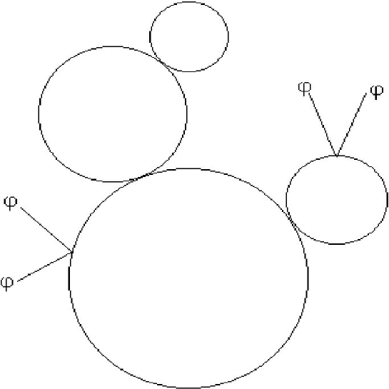
Figure 1: Generic 2PPR diagram

In this section, we will treat the unrenormalised 2PPI expansion and hence neglect all contributions from the counterterm Lagrangian. The way to get to the 2PPI expansion is to start from the 1PI expansion and sum all the seagull and bubble graphs. These insertions arise in 2PPR or two particle point reducible graphs because they disconnect from the rest of the diagram where two lines meeting at the same point (the 2PPR-point) are cut (fig. 1). We notice that seagull and bubble graphs contribute to the self energy as effective mass terms proportional to $\varphi_{i}\varphi_{j}$ and $\Delta_{ij}=\langle\phi_{i}\phi_{j}\rangle_{c}$ respectively. A short diagrammatical analysis suggests that all 2PPR insertions can be summed by simply deleting the 2PPR graphs from the 1PI expansion and introducing the effective mass :

$$\overline{m}^{2}_{ij}=m^{2}_{ij}+\lambda[\varphi_{i}\varphi_{j}+\Delta_{ij}]+\frac{\lambda}{2}[\varphi^{2}+\Delta_{kk}]\delta_{ij}$$ (3)

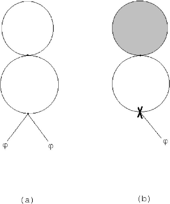
Figure 2: 2PPR part is shaded, 2PPI rest is earmarked

in the remaining 2PPI graphs. This is too naive though since there is a double counting problem which can be easily understood in the simple case of the 2 loop vacuum diagram (daisy graph with two petals) of fig. 2.a. Each petal can be seen as a selfenergy insertion in the other, so there is no way of distinguishing one or the other as the remaining 2PPI part. The trick which solves this combinatorial problem is to earmark one of the petals by applying a derivative with respect to $\varphi_{k}$ (fig. 2.b). This fixes the 2PPI remainder (which contains the earmark) in a unique way. Now, there are two ways in which the derivative can hit a $\varphi$ field. It can hit an explicit $\varphi$ field which is not a wing of a seagull or it can hit a wing of a seagull or implicit $\varphi$ field hidden in the effective mass. We therefore have

$$\frac{\delta}{\delta\varphi_{k}}\Gamma^{1PI}_{q}(m^{2},\varphi)=\frac{\partial}{\partial\varphi_{k}}\Gamma^{2PPI}_{q}(\overline{m}^{2},\varphi)+\left[\lambda\varphi_{k}\delta_{ij}+\lambda(\delta_{ik}\varphi_{j}+\delta_{jk}\varphi_{i})\right]\frac{\partial\Gamma^{2PPI}_{q}}{\partial\overline{m}^{2}_{ij}}(\overline{m}^{2},\varphi)$$ (4)

where $\Gamma^{1PI}=S(\varphi)+\Gamma^{1PI}_{q}$ or using the equation for the effective mass :

$$\frac{\delta}{\delta\varphi_{k}}\Gamma^{1PI}_{q}(m^{2},\varphi)=\frac{\delta}{\delta\varphi_{k}}\Gamma^{2PPI}_{q}(\overline{m}^{2},\varphi)-\left[\lambda\frac{\delta\Delta_{ij}}{\delta\varphi_{k}}+\frac{\lambda}{2}\delta_{ij}\frac{\delta\Delta_{\ell\ell}}{\delta\varphi_{k}}\right]\frac{\partial\Gamma^{2PPI}_{q}}{\partial\overline{m}^{2}_{ij}}(\overline{m}^{2},\varphi)$$ (5)

Using the same type of combinatorial argument, we have :

$$\frac{\partial\Gamma^{1PI}_{q}}{\partial m^{2}_{ij}}(m^{2},\varphi)=\frac{\partial\Gamma^{2PPI}_{q}}{\partial\overline{m}^{2}_{ij}}(\overline{m}^{2},\varphi)$$ (6)

and since

$$\frac{\Delta_{ij}}{2}=\frac{\partial\Gamma^{1PI}_{q}}{\partial m^{2}_{ij}}(m^{2},\varphi)$$ (7)

we find the following gap equation for $\Delta_{ij}$ :

$$\frac{\Delta_{ij}}{2}=\frac{\partial\Gamma^{2PPI}_{q}}{\partial\overline{m}^{2}_{ij}}(\overline{m}^{2},\varphi)$$ (8)

The gap equation (8) can be used to integrate (5) and we finally obtain

$$\Gamma^{1PI}(\overline{m}^{2},\varphi)=S(\varphi)+\Gamma^{2PPI}_{q}(\overline{m}^{2},\varphi)-\frac{\lambda}{8}\int d^{D}x\left((\Delta_{ii})^{2}+2(\Delta_{ij})^{2}\right)$$ (9)

This equation gives the 1PI effective action in terms of the 2PPI effective action and a term which corrects for double counting. The 2PPI effective action is just the 1PI effective action without 2PPR graphs and with the effective mass given by equation (3) running in the internal lines. For $m^{2}_{ij}=\delta_{ij}m^{2}$ we can make use of $O(N)$ symmetry to define :

$$\overline{m}^{2}_{ij}=\frac{\varphi_{i}\varphi_{j}}{\varphi^{2}}\overline{m}^{2}_{\sigma}+\left(\delta_{ij}-\frac{\varphi_{i}\varphi_{j}}{\varphi^{2}}\right)\overline{m}^{2}_{\pi}$$ (10)

and

$$\Delta_{ij}=\frac{\varphi_{i}\varphi_{j}}{\varphi^{2}}\Delta_{\sigma}+\left(\delta_{ij}-\frac{\varphi_{i}\varphi_{j}}{\varphi^{2}}\right)\Delta_{\pi}$$ (11)

so that the equation for the effective masses can be written as :

$$\overline{m}^{2}_{\sigma} = m^{2}+\frac{3\lambda}{2}\left[\varphi^{2}+\Delta_{\sigma}+\frac{N-1}{3}\Delta_{\pi}\right]$$

$$\overline{m}^{2}_{\pi} = m^{2}+\frac{\lambda}{2}\left[\varphi^{2}+\Delta_{\sigma}+(N+1)\Delta_{\pi}\right]$$ (12)

The relation between 1PI and 2PPI expansion now simplyfies to :

$$\Gamma^{1PI}(m^{2},\varphi) = S(\varphi)+\Gamma^{2PPI}_{q}(\overline{m}^{2}_{\sigma},\overline{m}^{2}_{\pi},\varphi)$$

$$- \frac{\lambda}{8}\int d^{D}x\left[3\Delta^{2}_{\sigma}+(N^{2}-1)\Delta^{2}_{\pi}+2(N-1)\Delta_{\sigma}\Delta_{\pi}\right]$$

and the gapequations are :

$$\frac{\delta\Gamma^{2PPI}}{\delta\overline{m}^{2}_{\sigma}} = \frac{\Delta_{\sigma}}{2}$$ (14)

$$\frac{\delta\Gamma^{2PPI}}{\delta\overline{m}^{2}_{\pi}} = (N-1)\frac{\Delta_{\pi}}{2}$$

Two remarks are in order here. The derivation given above is independent of temperature, so the relation (13) is also valid at finite T. Secondly, the masses $\overline{m}^{2}_{\sigma}$ and $\overline{m}^{2}_{\pi}$ are 2PPI effective masses. The physical $\sigma$ and $\pi$ masses $m^{2}_{\sigma}$ and $m^{2}_{\pi}$ still have to be calculated from the effective action (as poles of the propagators) and are not identical to these 2PPI effective masses.

3 Renormalisation of the 2PPI expansion

To be useful for practical calculations, we have to show that equation (4) which relates 1PI and 2PPI expansions and the gapequations (8) can be renormalised with the conventional counterterms. The crucial point in the proof of equations (4) and (8) was that the 2PPR insertions could be exactly summed via the effective 2PPI mass given in equation (3). For this to remain true after renormalisation, we have to use a mass independent renormalisation scheme. Therefore, in this paper, we will use minimal subtraction. Again, just as in the previous section, we will earmark the 1PI graphs by applying a $\varphi$ derivative so that 2PPR and 2PPI parts are unambiguous.

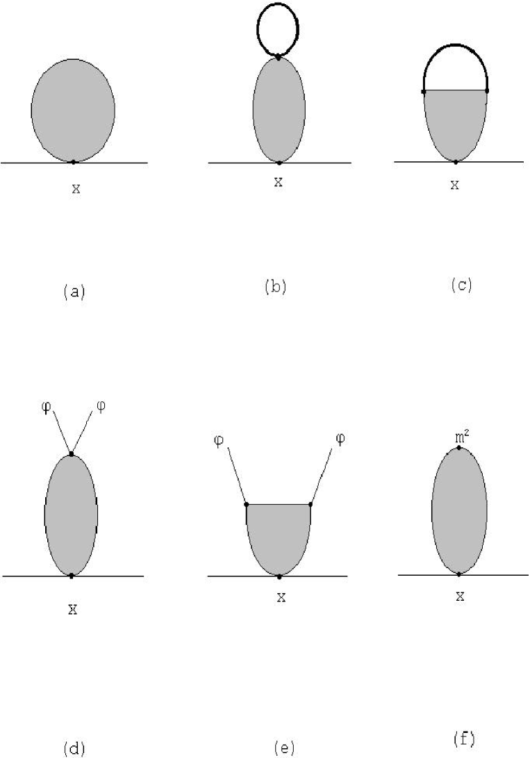
Figure 3: Generic bubble(shaded) and its subdivergences(shaded).Thick lines are full propagators.

We first renormalise the bubble subgraphs. Consider a generic bubble inserted at the 2PPR point $x$ (fig. 3.a). All primitively divergent subgraphs of the bubble graph which do not contain the 2PPR point $x$ can be renormalised with the counterterms of the $O(N)$ linear $\sigma$-model :

$$\delta\cal{L} = \delta Z\frac{1}{2}\partial_{\mu}\phi_{i}\partial_{\mu}\phi_{j}+\frac{1}{2}\delta Z^{ij;k\ell}_{2}m^{2}_{ij}\phi_{k}\phi_{\ell}$$

$$+ \frac{\lambda}{4!}\delta Z^{ijk\ell}_{\lambda}\phi_{i}\phi_{j}\phi_{k}\phi_{\ell}$$

where

$$\delta Z^{ijk\ell}_{\lambda}=\delta Z_{\lambda}\left(\delta_{ij}\delta_{k\ell}+\delta_{ik}\delta_{j\ell}+\delta_{i\ell}\delta_{jk}\right)$$ (16)

As a consequence of these subtractions, the contribution of the bubbles to the effective mass is proportional to $\langle\phi_{i}\phi_{j}\rangle_{c}$ where the connected V.E.V. is now calculated with the full Lagrangian, counterterms included. For subgraphs of the bubble which do contain the 2PPR point $x$, we need only the 2PPR-parts of the counterterm. This means those parts which correspond to subtractions for subgraphs which disconnect from the rest of the graph when two lines meeting at the 2PPR point $x$ are cut. Let’s first renormalise the proper subgraphs of the bubble which contain $x$. Their generic topology is displayed in fig. 3.b and 3.c. They can be made finite with the 2PPR part $\left(\frac{1}{2!}\right)^{2}\delta Z^{ij;k\ell}_{\lambda,2PPR}\phi_{i}\phi_{j}\phi_{k}\phi_{\ell}$ where the lines meeting at the 2PPR point $x$ carry the O(N) indices i and j. Their contribution to the effective mas $m^{2}_{ij}$ is given by $\frac{1}{2}\delta Z^{ij;k\ell}_{\lambda,2PPR}\langle\phi_{k}\phi_{\ell}\rangle_{c}$. We still have to subtract the overal divergences of the bubble graph. Their generic topology is displayed in fig. 3.d and 3.e for coupling constant renormalisation and fig. 3.f for mass renormalization. Again only the 2PPR parts of the counterterm contributions have to be included and the overall divergences contribute $\frac{\lambda}{2}\delta Z^{ij;k\ell}_{\lambda,2PPR}\varphi_{k}\varphi_{\ell}+\delta Z^{ij;k\ell}_{2,2PPR}m^{2}_{k\ell}$. Adding the various contributions coming from renormalizing the bubble graphs, we find for the renormalised effective mass :

$$\overline{m}^{2}_{R,ij} = m^{2}_{ij}+\lambda\left[\varphi_{i}\varphi_{j}+\Delta_{ij}\right]+\frac{\lambda}{2}\left[\varphi^{2}+\Delta_{kk}\right]\delta_{ij}$$ (17)

$$+ \delta Z^{ij;k\ell}_{2,2PPR}m^{2}_{k\ell}+\frac{\lambda}{2}\delta Z^{ij;k\ell}_{\lambda,2PPR}\left[\Delta_{k\ell}+\varphi_{k}\varphi_{\ell}\right]$$

where $\Delta_{ij}=\langle\phi_{i}\phi_{j}\rangle_{c}$ and the V.E.V. is calculated with inclusion of the counterterms.

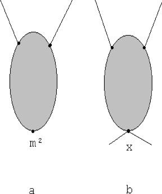
Figure 4: Generic diagram for mass renormalisation (a) and generic 2PPR coupling constant renormalisation diagram (b)

Because we use a mass independent renormalization scheme, the 2PPR part of coupling constant renormalisation can be related to multiplicative mass renormalisation. Indeed lets consider a generic diagram for mass renormalisation which is proportional to $m^{2}_{pq}$ (fig. 4.a). On the other hand, lets consider in fig. 4.b a generic 2PPR coupling constant renormalisation graph inserted at the 2PPR point $x$. The latter can be gotten from the former by replacing the mass $m^{2}_{pq}$ by the coupling constant $\lambda_{pqij}$ and summing over p and q. Therefore we have:

$$\lambda\delta Z^{ij;k\ell}_{\lambda,2PPR}=\lambda\left(\delta_{ij}\delta_{pq}+\delta_{ip}\delta_{jq}+\delta_{iq}\delta_{jp}\right)\delta Z^{pq;k\ell}_{2}$$ (18)

or

$$\delta Z^{ij;k\ell}_{\lambda,2PPR}=\delta_{ij}\delta Z^{pp;k\ell}_{2}+2\delta Z^{ij;k\ell}_{2}$$ (19)

In an analogous way, we can relate the 2PPR part of multiplicative mass renormalisation to vacuum energy renormalisation. In minimal subtraction, vacuum diagrams are logaritmically divergent and proportional to $m^{4}$. Their divergences are cancelled with the counterterm :

$$\delta E_{vac}=\frac{1}{2}\overline{m}^{2}_{ij}\overline{m}^{2}_{k\ell}\delta\zeta^{ij;k\ell}$$ (20)

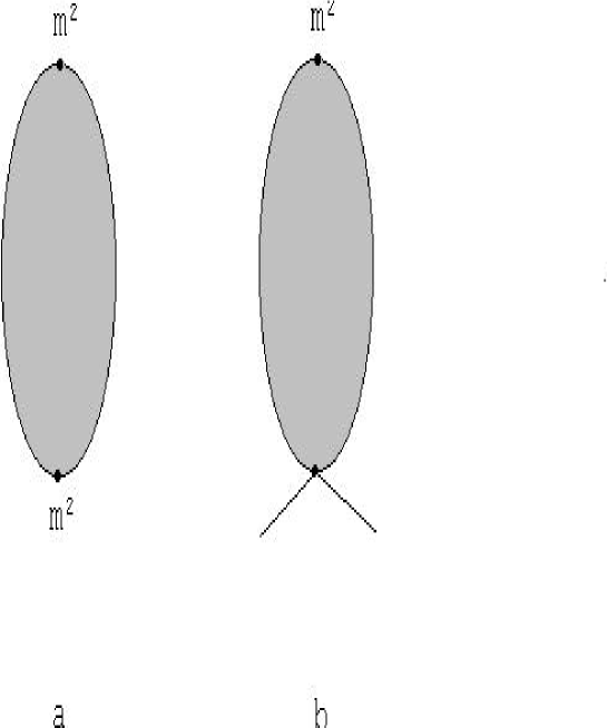
Figure 5: Generic divergent vacuum diagram (a) and generic 2PPR mass renormalisation diagram (b)

A generic divergent vacuum graph proportional to $m^{4}$ is given in fig. 5.a. A generic 2PPR part of mass renormalisation is given in fig. 5.b. Just as in the previous case, it is clear that

$$\delta Z^{ij;k\ell}_{2,2PPR}=\lambda\left(\delta_{ij}\delta_{pq}+\delta_{ip}\delta_{jq}+\delta_{iq}\delta_{jp}\right)\delta\zeta^{pq;k\ell}$$ (21)

or

$$\delta Z^{ij;k\ell}_{2,2PPR}=\lambda\left(\delta_{ij}\delta\zeta^{pp;k\ell}+2\delta\zeta^{ij;k\ell}\right)$$ (22)

Using (19) and (22) the renormalised effective mass given by (17) can be written as :

$$\overline{m}^{2}_{R,ij}=m^{2}_{ij} + \lambda\left[Z^{ij,k\ell}_{2}(\varphi_{k}\varphi_{\ell}+\Delta_{k\ell})+2\delta\zeta^{ij;k\ell}m^{2}_{k\ell}\right]$$ (23)

$$+ \frac{\lambda}{2}\left[Z^{pp;k\ell}_{2}(\varphi_{k}\varphi_{\ell}+\Delta_{k\ell})+2\delta\zeta^{pp;k\ell}m^{2}_{k\ell}\right]$$

where

$$Z^{ij;k\ell}_{2}=\frac{1}{2}\left(\delta_{ik}\delta_{j\ell}+\delta_{i\ell}\delta_{jk}\right)+\delta Z^{ij;k\ell}_{2}$$ (24)

If we introduce the renormalised local composite operators

$$\langle\phi_{i}\phi_{j}\rangle_{c,R}=\Delta_{ij,R}=Z^{ij;k\ell}_{2}\Delta_{k\ell}+\delta Z^{ij;k\ell}_{2}\varphi_{k}\varphi_{\ell}+2\delta\zeta^{ij;k\ell}m^{2}_{k\ell}$$ (25)

the renormalised effective mass finally becomes :

$$\overline{m}^{2}_{R,ij}=m^{2}_{ij}+\lambda\left(\varphi_{i}\varphi_{j}+\Delta_{R,ij}\right)+\frac{\lambda}{2}\left(\varphi^{2}+\Delta_{R,kk}\right)\delta_{ij}$$ (26)

From this equation, it follows that $\Delta_{R,ij}$ must be finite.

Once we have renormalised the bubble subgraphs, the $\varphi$ derivative of $\Gamma^{1PI}_{q}$ can be written as :

$$\frac{\delta}{\delta\varphi_{k}}\Gamma^{1PI}_{q,BR}=\frac{\partial}{\partial\varphi_{k}}\Gamma^{2PPI}_{q}(\overline{m}^{2}_{R},\varphi)+\left[\lambda\varphi_{k}\delta_{ij}+\lambda\left(\delta_{ik}\varphi_{j}+\delta_{jk}\varphi_{i}\right)\right]\frac{\partial\Gamma^{2PPI}_{q}}{\partial\overline{m}^{2}_{R,ij}}(\overline{m}^{2}_{R},\varphi)$$ (27)

where BR stands for bubble renormalised. Because there is no overlap, having renormalised the bubble subgraphs, we can now renormalize the 2PPI remainder (which contains the earmarked vertex). Let us first consider mass renormalization. A subgraph $\gamma$ in the 2PPI remainder of $\frac{\delta}{\delta\varphi_{k}}\Gamma^{1PI}_{q,BR}$ that needs mass renormalisation can be made finite with a counterterm $\delta Z^{ij;k\ell}_{2}(\gamma)m^{2}_{ij}\phi_{k}\phi_{\ell}/2$. However for any such subgraph $\gamma$, there are subgraphs $\gamma^{\prime}$ obtained from $\gamma$ by replacing the mass $m^{2}_{ij}$ with a seagull or renormalised bubble. These subgraphs require coupling constant renormalization which entails a counterterm $\delta Z^{ij;k\ell}_{\lambda,2PPR}\frac{\lambda}{2}(\varphi_{i}\varphi_{j}+\Delta_{R,ij})\phi_{k}\phi_{\ell}/2$. Taking into account the identity (19) of renormalization constants for mass renormalisation and 2PPR coupling constant renormalization, the effective counterterm for the mass-type divergent subgraphs adds up to :

$$\frac{1}{2}\delta Z^{ij;k\ell}_{2}(\gamma)m^{2}_{ij}\phi_{k}\phi_{\ell} + \frac{1}{2}\left(\delta_{ij}\delta Z^{pp;k\ell}_{2}(\gamma)+2\delta Z^{ij;k\ell}_{2}(\gamma)\right)\frac{\lambda}{2}(\varphi_{i}\varphi_{j}+\Delta_{R,ij})\phi_{k}\phi_{\ell}$$ (28)

$$= \frac{1}{2}\delta Z^{ij;k\ell}_{2}(\gamma)\left[m^{2}_{ij}+\lambda[\varphi_{i}\varphi_{j}+\Delta_{R,ij}]+\frac{\lambda}{2}(\varphi^{2}+\Delta_{R,\ell\ell})\delta_{ij}\right]\phi_{k}\phi_{\ell}$$

$$= \frac{1}{2}\delta Z^{ij;k\ell}_{2}(\gamma)\overline{m}^{2}_{R,ij}\phi_{k}\phi_{\ell}$$

which is exactly what is needed for mass renormalization of $\Gamma^{2PPI}_{q}(\overline{m}^{2}_{R},\varphi)$ in the right hand side of (27). The remaining divergent subgraphs need wave function renormalization or are of the coupling constant renormalization type that cannot be generated by inserting seagulls or bubbles in mass-type divergent subgraphs. They are made finite by counterterms independent of mass and hence are the same for left and right hand sides of equation (27). Therefore we can conclude that in a mass independent renormalisation scheme, equation (4) can be renormalised with the available counterterms as :

$$\frac{\delta}{\delta\varphi_{k}}\Gamma^{1PI}_{q,R}(m^{2},\varphi)=\frac{\partial}{\partial\varphi_{k}}\Gamma^{2PPI}_{q,R}(\overline{m}^{2}_{R},\varphi)+\left[\lambda\varphi_{k}\delta_{ij}+\lambda(\delta_{ik}\varphi_{j}+\delta_{jk}\varphi_{i})\right]\frac{\partial\Gamma^{2PPI}_{q,R}}{\partial\overline{m}^{2}_{R,ij}}$$ (29)

To proceed, we have to renormalize the gapequations (8). Using essentially the same arguments as in the previous paragraphs, we find that

$$\frac{\partial\Gamma^{1PI}_{q,R}}{\partial m^{2}_{ij}}(m^{2},\varphi)=\frac{\partial\Gamma^{2PPI}_{q,R}}{\partial\overline{m}^{2}_{R,ij}}(\overline{m}^{2}_{R},\varphi)$$ (30)

From the pathintegral, we readily obtain :

$$\frac{\partial\Gamma^{1PI}_{q,R}}{\partial m^{2}_{ij}}(m^{2},\varphi) = \frac{1}{2}Z^{ij;k\ell}_{2}(\varphi_{k}\varphi_{\ell}+\langle\phi_{k}\phi_{\ell}\rangle_{c})+\frac{\partial}{\partial m^{2}_{ij}}\delta E_{vac}$$ (31)

$$= \frac{1}{2}\left(\varphi_{i}\varphi_{j}+Z^{ij;k\ell}_{2}\Delta_{k\ell}+\delta Z^{ij;k\ell}_{2}\varphi_{k}\varphi_{\ell}+2\delta\zeta^{ij;k\ell}m^{2}_{k\ell}\right)$$

$$= \frac{1}{2}(\varphi_{i}\varphi_{j}+\Delta_{R,ij})$$

where we used (20) and (25). Since $\Gamma^{1PI}_{R}$ is finite it follows that $\Delta_{R,ij}$ is finite. This reconfirms our analysis of bubble renormalization where from the finiteness of the renormalised effective mass (eq.(26)), we concluded that $\Delta_{R,ij}$ defined by (25) is finite. Using $\frac{\partial}{\partial m^{2}_{ij}}\Gamma^{1PI}_{R}=\varphi_{i}\varphi_{j}/2+\frac{\partial}{\partial m^{2}_{ij}}\Gamma^{1PI}_{q,R}$ and equations (30) and (31) we finally obtain the renormalised gap equations :

$$\frac{\Delta_{R,ij}}{2}=\frac{\partial\Gamma^{2PPI}_{q,R}}{\partial\overline{m}^{2}_{R,ij}}(\overline{m}^{2}_{R},\varphi)$$ (32)

As in the unrenormalised case, these gap equations can be used to integrate (29) :

$$\Gamma^{1PI}_{R}(m^{2},\varphi)=S(\varphi)+\Gamma^{2PPI}_{q,R}\left(\overline{m}^{2}_{R},\varphi\right)-\frac{\lambda}{8}\int d^{D}x\left[(\Delta_{R,ii})^{2}+(2\Delta_{R,ij})^{2}\right]$$ (33)

Our renormalised equation (33) together with the renormalised gap equations (32) enable us to sum seagulls and bubble graphs in such a way that perturbative renormalisability is preserved. To renormalise $\Gamma^{1PI}$, it is sufficient to renormalize $\Gamma^{2PPI}$ using a mass independent renormalisation scheme such as MS, calculate the renormalised local composite operators $\Delta_{R,ij}$ from the gap equations, and substitute them back in (33). The advantage of the 2PPI expansion is that with the same (or even less) calculational effort as goes into the perturbative calculation of $\Gamma^{1PI}$, the seagull and bubble graphs are summed order by order. The gap equations are local and can easily be solved numerically.

The previous analysis was independent of temperature. Because $\Gamma^{1PI}$ can be renormalised at finite T with the counterterms at T = 0, the same goes through for $\Gamma^{2PPI}$. Therefore, our renormalised equations (32) and (33) are valid at finite T.

4 Goldstone’s theorem

If we choose $m^{2}_{ij}=m^{2}\delta_{ij}$, we can use of the O(N) symmetry to define the renormalised effective masses $m_{R,\sigma}$ and $m_{R,\pi}$ and renormalised composite operators $\Delta_{R,\sigma}$ and $\Delta_{R,\pi}$ as :

$$\overline{m}^{2}_{R,ij}=\frac{\varphi_{i}\varphi_{j}}{\varphi^{2}}\overline{m}^{2}_{R,\sigma}+\left(\delta_{ij}-\frac{\varphi_{i}\varphi_{j}}{\varphi^{2}}\right)\overline{m}^{2}_{R,\pi}$$ (34)

$$\Delta_{R,ij}=\frac{\varphi_{i}\varphi_{j}}{\varphi^{2}}\Delta_{R,\sigma}+\left(\delta_{ij}-\frac{\varphi_{i}\varphi_{j}}{\varphi^{2}}\right)\Delta_{R,\pi}$$ (35)

so that equation (3) becomes :

$$\overline{m}^{2}_{R,\sigma} = m^{2}+\frac{3\lambda}{2}\left[\varphi^{2}+\Delta_{R,\sigma}+\frac{N-1}{3}\Delta_{R,\pi}\right]$$ (36)

$$\overline{m}^{2}_{R,\pi} = m^{2}+\frac{\lambda}{2}\left[\varphi^{2}+\Delta_{R,\sigma}+(N+1)\Delta_{R,\pi}\right]$$

Because of O(N) symmetry, $\overline{m}^{2}_{R,\sigma},\overline{m}^{2}_{R,\pi},\Delta_{R,\sigma}$ and $\Delta_{R,\pi}$ are O(N) invariant functions of $\varphi_{i}$. The relation between the renormalised 1PI and 2PPI expansion now simplifies to :

$$\Gamma^{1PI}(m^{2},\varphi) = S(\varphi)+\Gamma^{2PPI}_{q,R}\left(\overline{m}^{2}_{R,\sigma},m^{2}_{R,\pi},\varphi\right)$$

$$- \frac{\lambda}{8}\int d^{D}x\left[3\Delta^{2}_{R,\sigma}+(N^{2}-1)\Delta^{2}_{R,\pi}+2(N-1)\Delta_{R,\sigma}\Delta_{R,\pi}\right]$$

and the gapequations become :

$$\frac{\delta\Gamma^{2PPI}_{q,R}}{\delta\overline{m}^{2}_{R,\sigma}} = \frac{\Delta_{R,\sigma}}{2}$$

$$\frac{\delta\Gamma^{2PPI}}{\delta\overline{m}^{2}_{R,\pi}} = (N-1)\frac{\Delta_{R,\pi}}{2}$$ (38)

Since because of O(N) symmetry, the effective masses $\overline{m}_{R,\sigma}$ and $\overline{m}_{R,\pi}$ and the composite operators $\Delta_{R,\sigma}$ and $\Delta_{R,\pi}$ are O(N) invariant, Goldstone’s theorem must be obeyed at any loop order of the 2PPI expansion. To check this explicitely, we should not make the mistake of identifying the effective mass $\overline{m}_{R,\pi}$ with the real physical pion mass $m_{\pi}$, defined as the pole in the pion propagator. This pole should occur at $p^{2}=0$ and hence we can use the effective action at $p=0$, i.e. the effective 1PI potential. Using (37), the renormalised 1PI effective potential becomes :

$$V^{1PI}_{R}(m^{2},\varphi) = V(\varphi)+V^{2PPI}_{q,R}\left(\overline{m}^{2}_{R,\sigma},\overline{m}^{2}_{R,\pi},\varphi^{2}\right)$$ (39)

$$- \frac{\lambda}{8}\left(3\Delta^{2}_{R,\sigma}+(N^{2}-1)\Delta^{2}_{R,\pi}+2(N-1)\Delta_{R,\sigma}\Delta_{R,\pi}\right)$$

Since $V^{2PPI}_{q,R}$ is O(N) invariant we can use the standard argument to show that $\frac{\partial^{2}V^{1PI}}{\partial\varphi_{i}\partial\varphi_{j}}$ has N-1 zero eigenvalues at any order of the 2PPI loop expansion. More explicitely we find from (35), (36) and (38) that

$$\frac{\partial V^{1PI}_{R}}{\partial\varphi_{i}}=\varphi_{i}\left(m^{2}+\frac{\lambda}{2}\varphi^{2}+\frac{3\lambda}{2}\left(\Delta_{R,\sigma}+\frac{N-1}{3}\Delta_{R,\pi}\right)+2\frac{\partial V^{2PPI}_{q,R}}{\partial\varphi^{2}}\right)$$ (40)

and

$$\frac{\partial^{2}V^{1PI}_{R}}{\partial\varphi_{i}\partial\varphi_{j}} = \delta_{ij}\left(m^{2}+\frac{\lambda\varphi^{2}}{2}+\frac{3\lambda}{2}\left(\Delta_{R,\sigma}+\frac{N-1}{3}\Delta_{R,\pi}\right)+2\frac{\partial V^{2PPI}_{q,R}}{\partial\varphi^{2}}\right)$$ (41)

$$+ \lambda\varphi_{i}\varphi_{j}\left[1+3\frac{\partial\Delta_{R,\sigma}}{\partial\varphi^{2}}+(N-1)\frac{\partial\Delta_{R,\pi}}{\partial\varphi^{2}}+4\frac{\partial^{2}V^{2PPI}_{q,R}}{(\partial\varphi^{2})^{2}}\right]$$

So, we have N-1 massless particles if

$$m^{2}_{\pi}=m^{2}+\frac{\lambda}{2}\varphi^{2}+\frac{3\lambda}{2}\left(\Delta_{R,\sigma}+\frac{N-1}{3}\Delta_{R,\pi}\right)+2\frac{\partial V^{2PPI}_{q,R}}{\partial\varphi^{2}}=0$$ (42)

Using (40) we conclude that the masslessness of the pions is nothing else than the equation of motion in the case of spontaneous symmetry breaking.

5 The effective potential at finite temperature

In this section, we will calculate the effective potential at finite T using the 2PPI expansion at one loop. Since there are (N-1) effective masses $\overline{m}_{R,\pi}$ and one mass $\overline{m}_{R,\sigma}$ running in the one loop vacuum diagram, we have

$$V^{2PPI}_{q}\left(\overline{m}^{2}_{R,\sigma},\overline{m}^{2}_{R,\pi},\varphi^{2}\right)=\frac{1}{2}\sum\int\ln(k^{2}+\overline{m}^{2}_{R,\sigma})+\frac{N-1}{2}\sum\int\ln(k^{2}+\overline{m}^{2}_{R,\pi})$$ (43)

where

$$\sum\int=T\sum_{\omega_{n}}\int\frac{d^{3}p}{(2\pi)^{3}}$$ (44)

and the Matsubara frequencies are denoted by $\omega_{n}$. We can simply renormalise $V^{2PPI}_{q}$ using for example the $\overline{MS}$ scheme and calculate the renormalised V.E.V. of the composite operators from the gapequations (38). We find at one loop :

$$V^{2PPI}_{q,R} = \frac{\overline{m}^{4}_{R,\sigma}}{64\pi^{2}}\left(\ln\frac{\overline{m}^{2}_{R,\sigma}}{\overline{\mu}^{2}}-\frac{3}{2}\right)+(N-1)\frac{\overline{m}^{4}_{R,\pi}}{64\pi^{2}}\left(\ln\frac{\overline{m}^{2}_{R,\pi}}{\overline{\mu}^{2}}-\frac{3}{2}\right)$$ (45)

$$+ Q_{T}(\overline{m}_{R,\sigma})+(N-1)Q_{T}(\overline{m}_{R,\pi})$$

where

$$Q_{T}(m)=T\int\frac{d^{3}q}{(2\pi)^{3}}\ln\left(1-e^{-\frac{\omega_{q}}{T}}\right)$$ (46)

The effective 1PI potential then reads :

$$V^{1PI}_{R}(m^{2},\varphi) = \frac{m^{2}}{2}\varphi^{2}+\frac{\lambda}{8}\varphi^{4}+\frac{\overline{m}^{4}_{R,\sigma}}{64\pi^{2}}\left(\ln\frac{\overline{m}^{2}_{R,\sigma}}{\overline{\mu}^{2}}-\frac{3}{2}\right)$$ (47)

$$+ (N-1)\frac{\overline{m}^{4}_{R,\pi}}{64\pi^{2}}\left(\ln\frac{\overline{m}^{2}_{R,\pi}}{\overline{\mu}^{2}}-\frac{3}{2}\right)+Q_{T}(\overline{m}_{R,\sigma})+(N-1)Q_{T}(\overline{m}_{R,\pi})$$

$$- \frac{\lambda}{8}\left(3\Delta^{2}_{R,\sigma}+(N^{2}-1)\Delta^{2}_{R,\pi}+2(N-1)\Delta_{R,\sigma}\Delta_{R,\pi}\right)$$

with

$$\Delta_{R,\ast} = \sum\int\frac{1}{k^{2}+\overline{m}^{2}_{R,\ast}}$$ (48)

$$= \frac{\overline{m}^{2}_{R,\ast}}{16\pi^{2}}\left(\ln\frac{\overline{m}^{2}_{R,\ast}}{\overline{\mu}^{2}}-1\right)+P_{T}(\overline{m}_{R,\ast})$$

where

$$P_{T}(m)=2\frac{\partial}{\partial m^{2}}Q_{T}(m^{2})=\int\frac{d^{3}q}{(2\pi)^{3}}\frac{n_{B}(\omega_{q})}{\omega_{q}}$$ (49)

Our expression (47) together with the gapequations (48) and the definition of the effective masses (36) completely agree with previously published results [4,10] obtained using the CJT approach at the daisy and superdaisy order (2PI expansion). The advantage of our 2PPI expansion is that we arrive quite simply and naturally at this result keeping only the one loop term while the 2PI approach has to keep part of the 2 loop graphs (the two bubble graph) and the simple expression (47) is only obtained after some rearrangement. Furthermore, one can easily calculate higher order terms in the 2PPI expansion while in the 2PI expansion, it is very difficult to go beyond the Hartree approximation because of the non-locality of the gapequations.

In our approach, renormalisation of the non-perturbative results is straightforward. This is because we renormalise the effective 2PPI potential and hence the gapequations before we try solving them. If one does it the other way around as in [4], perturbative renormalizability is apparently spoiled. This is because in the resummation (see section 3), parts of the counterterms (the 2PPR parts) have to be included at all orders, and it is very difficult if not impossible to do this once the gapequations are solved and whole classes of diagrams have already been summed.

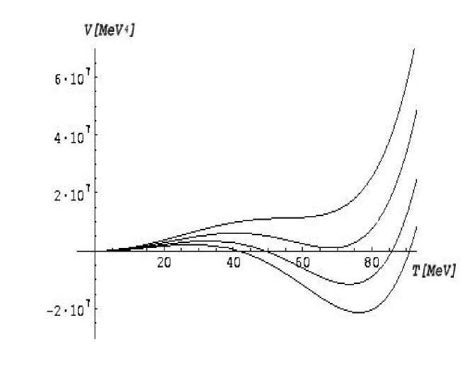
Figure 6: Effective potential $V(\varphi)$ at $T=186,192,200,208$ for $\lambda=\frac{90.2}{3}$.

As to our numerical results, they coincide (at least for that part concerning the effective potential) with the CJT results obtained for example in [10]. We take the N=4 Gell-Mann Levy linear $\sigma$-model, relevant for QCD and use the parameter choice of Nemoto et al. [10]: $\lambda=\frac{90.2}{3}$ (our $\lambda$ differs from the one in [10] by a factor of 3 at N=4) $\overline{\mu}=320$ MeV, $m^{2}=-122375\mbox{MeV}^{2}$. Our results are in the chiral limit. Extension to real pion masses is trivial. In fig. 6, we display the effective potential at T = 186, 192, 200 and 208 MeV. We clearly see a first order phase transition around $T_{c}=200\mbox{MeV}$. This agrees with other mean field approaches [15,16,5]. The renormalisation group however, leads us to believe that the actual phase transition of the O(4) linear sigma model should be second order. There are suggestions [10] that inclusion of the 2 loop setting sun diagram should change the phase transition from first to second order, at least for small $\lambda$. However this is very difficult to check in the CJT formalism because of the non-local nature of the gap equations. In our 2PPI approach, this should be no problem and work concerning this issue is in progress [17].

6 The $\sigma$-meson mass

Because of its relevance in the context of ultrarelativistic heavy-ion collisions, the $\sigma$-resonance has been thoroughly studied in various models [18,19,6,10]. In the CJT approach to the O(4) linear $\sigma$-model, the $\sigma$-meson mass has been studied in [10] and defined via the effective potential. The physical $\sigma$-meson however, is defined via the effective action as solution of the mass equation

$$\int d^{4}xe^{ip(x-y)}\frac{\delta^{2}\Gamma}{\delta\varphi_{j}(y)\delta\varphi_{i}(x)}=0$$ (50)

for $-p^{2}$. At finite temperature, the propagators are no longer Lorentz invariant. They are functions of $p^{2}_{0}$ and $\vec{p}^{2}$ instead of $p^{2}$. The standard prescription is to define mass at rest with respect to the heatbath, this means putting $\vec{p}^{2}=0$ and solving (50) for $-p^{2}_{0}$. Using the fact that at one loop the 2PPI effective action only depends on $\varphi_{i}$ through the effective masses, it follows from (37) and the gapequations (38) that

$$\frac{\delta^{2}\Gamma}{\delta\varphi_{j}(y)\delta\varphi_{i}(x)} = \left[-\partial^{2}+m^{2}+\frac{\lambda}{2}\varphi^{2}(x)+\frac{3\lambda}{2}\left(\Delta_{R,\sigma}(x)+\frac{N-1}{3}\Delta_{R,\pi}(x)\right)\delta_{ij}\right.$$

$$+ \left.\lambda\varphi_{i}(x)\varphi_{j}(y)\right]\delta(x-y)+\frac{3\lambda}{2}\varphi_{i}(x)\left[\frac{\delta\Delta_{R,\sigma}(x)}{\delta\varphi_{j}(y)}+\frac{N-1}{3}\frac{\delta\Delta_{\pi}(x)}{\delta\varphi_{j}(y)}\right]$$

If we choose $\varphi_{i}=\delta_{iN}\varphi$ and use equation (36) for $\overline{m}^{2}_{R,\sigma}$, we can rewrite the $\sigma$-massequation as :

$$p^{2}+\overline{m}^{2}_{R,\sigma}+3\lambda\varphi^{2}\left(\Delta_{R,\sigma}^{\prime}(p)+\frac{N-1}{3}\Delta^{\prime}_{R,\pi}(p)\right)=0$$ (52)

with

$$\Delta^{\prime}_{R,\ast}(p)=\int d^{4}xe^{ip(x-y)}\frac{\partial\Delta_{R,\ast}(x)}{\partial\varphi^{2}(y)}$$ (53)

From the equation of motion (42) at one loop and equation (36) it follows that $\overline{m}^{2}_{R,\sigma}=\lambda\varphi^{2}$ which is the tree-level mass of the $\sigma$-meson (the condensate $\varphi$ is of course determined by the full expression (42) containing quantum corrections). Therefore the self energy of the $\sigma$-meson at one loop in the 2PPI expansion is given by :

$$\Sigma_{\sigma}(p)=3\lambda\varphi^{2}\left(\Delta^{\prime}_{R,\sigma}(p)+\frac{N-1}{3}\Delta^{\prime}_{R,\pi}(p)\right)$$ (54)

This selfenergy can be calculated exactly. From equation (48) we have

$$\Delta^{\prime}_{R,\ast}(p)=-B_{\ast}\frac{\partial\overline{m}^{2}_{R,\ast}}{\partial\varphi^{2}}$$ (55)

where

$$B_{\ast}=B(\overline{m}^{2}_{R,\ast},p)=\Sigma\int\frac{1}{q^{2}+\overline{m}^{2}_{R,\ast}}\frac{1}{(q+p)^{2}+\overline{m}^{2}_{R,\ast}}$$ (56)

From (55) and the effective mass equations (36) we derive the system

$$\Delta^{\prime}_{R,\sigma} = -B_{\sigma}\left(\frac{3\lambda}{2}+\frac{3\lambda}{2}\Delta^{\prime}_{R,\sigma}+\frac{\lambda}{2}(N-1)\Delta^{\prime}_{R,\pi}\right)$$

$$\Delta^{\prime}_{R,\pi} = -B_{\pi}\left(\frac{\lambda}{2}+\frac{\lambda}{2}\Delta^{\prime}_{R,\sigma}+\frac{\lambda}{2}(N+1)\Delta^{\prime}_{R,\pi}\right)$$ (57)

This system can be easily solved and we finally obtain for the self energy of the $\sigma$-meson :

$$\Sigma_{\sigma}(p)=-\lambda^{2}\varphi^{2}\frac{9B_{\sigma}+(N-1)B_{\pi}+3\lambda(N+2)B_{\sigma}B_{\pi}}{2+3\lambda B_{\sigma}+\lambda(N+1)B_{\pi}+\lambda^{2}(N+1)B_{\sigma}B_{\pi}}$$ (58)

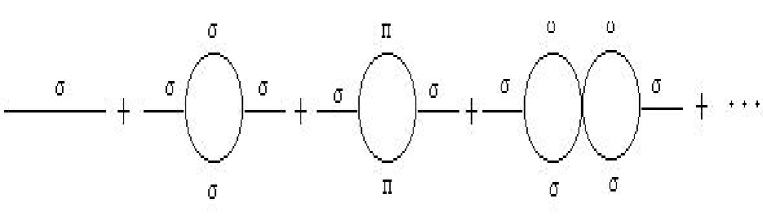
Figure 7: Feynman diagrams contributing to $\sigma$ - propagator at one loop in the 2PPI expansion

Adding the effective mass $\overline{m}^{2}_{R,\sigma}$ (which runs in the tree level propagators of the 2PPI expansion) to the one loop 2PPI selfenerg (58), we find we have summed an infinite series of Feynman diagrams given in fig. 7. The propagators in the internal lines are $\sigma$ as well as $\pi$-propagators and they carry effective masses $\overline{m}_{R,\sigma}$ and $\overline{m}_{R,\pi}$. This sum goes beyond the daisy-superdaisy approximation which is given by the first term only. In fact we have summed all 2PPR contributions to the selfenergy which can be made from one loop 2PPI subdiagrams. This is of course consistent with the fact that we have calculated the $\sigma$-meson propagators from the one loop 2PPI effective action.

In the same way, we can calculate the one loop 2PPI mass of the pion. Our one loop 2PPI approximation again goes beyond the daisy-superdaisy result and we find that the selfenergy is just enough to make the pion mass exactly zero. This is of course easily understood as the effective action at p = 0 is nothing else than the effective potential and we have already shown on general grounds in section 4 that the second derivative of the effective potential with respect to the pion fields is zero at the minimum of the potential.

To obtain numerical results we have to evaluate $B(\overline{m}^{2}_{R,\ast},p)$ at finite T. Using dimensional regularisation and the $\overline{MS}$ scheme, we find

$$B_{R}(m^{2},p)=-\frac{1}{16\pi^{2}}\left[\ln\frac{m^{2}}{\overline{\mu}^{2}}+\sqrt{1+\frac{4m^{2}}{p^{2}}}\ln\left(\frac{\sqrt{1+\frac{4m^{2}}{p^{2}}}+1}{\sqrt{1+\frac{4m^{2}}{p^{2}}}-1}\right)-2\right]+B_{T}(m^{2},p)$$

with

$$B_{T}(m^{2},p) = \int\frac{d^{3}q}{(2\pi)^{3}}n_{B}(\omega_{\bf q})\frac{1}{\omega_{\bf q}}\frac{\omega^{2}_{\bf{q+p}}-\omega^{2}_{\bf q}+p^{2}_{0}}{(\omega^{2}_{\bf{q+p}}-\omega^{2}_{\bf q}+p^{2}_{0})^{2}+4\omega^{2}_{\bf q}p^{2}_{0}}$$ (60)

$$+ n_{B}(\omega_{\bf{q+p}})\frac{1}{\omega_{\bf q+p}}\frac{-\omega^{2}_{\bf{q+p}}+\omega^{2}_{\bf q}+p^{2}_{0}}{(-\omega^{2}_{\bf{q+p}}+\omega^{2}_{\bf q}+p^{2}_{0})^{2}+4\omega^{2}_{\bf{q+p}}p^{2}_{0}}$$

We determine the $\sigma$-meson mass as the zero in $p^{2}_{0}(\overline{p}^{2}=0)$ of the real part of the inverse $\sigma$-propagator $p^{2}+\overline{m}^{2}_{R,\sigma}+Re(\Sigma_{\sigma}(p^{2}_{0},\vec{p}^{2}=0))$. We again use the parameters $\lambda=90.2/3,\overline{\mu}=320\mbox{MeV},m^{2}=-122375\mbox{MeV}^{2}$. In Nemoto et al [10], the $\sigma$-meson mass was determined from the effective potential and the parameters were chosen such that $m_{\sigma}=600\mbox{MeV}$ at T = 0. Our more physical definition of the $\sigma$-mass gives $m_{\sigma}=548.3\mbox{MeV}$ at T = 0. So the correct definition of mass only gives a 10% change and therefore, this choice of parameters is acceptable given the ambiguity in the experimental value for the $\sigma$-meson mass. In fig. 8 we display the physical $\sigma$-meson mass (zero in $p^{2}_{0}$ of $p^{2}_{0}+\overline{m}^{2}_{R,\sigma}+Re(\Sigma_{\sigma}(p_{0},\vec{0}))$ and the $\sigma$-meson mass as determined from the effective potential and equal to $\overline{m}^{2}_{R,\sigma}+\Sigma_{\sigma}(0,\vec{0})$, at finite temperature. The influence of temperature is to decrease to $\sigma$-meson mass, a well known effect established with other methods [6] or in other models [18,19].

7 Summary and conclusions

In this paper, we have studied the O(N) linear $\sigma$-model at finite temperature using the 2PPI expansion. We have shown that at one loop order in this expansion, the Hartree result is reproduced in a very efficient way. We have given an all orders proof that this expansion can be renormalised with the usual counterterms if a mass independent renormalisation scheme is used. We have shown that at finite temperature and each order of the 2PPI expansion, Goldstone’s theorem is obeyed. We have calculated the effective potential for N =4 and found a first order phase transition as was to be expected from a mean field approximation. However, whereas previous methods to obtain the Hartree result such as the CJT formalism are very difficult to apply beyond the mean field level, the 2PPI expansion is ideally suited to investigate post-Hartree corrections to various thermodynamical quantities. For example, we calculated the one loop 2PPI result for the $\sigma$-meson mass and showed that it sums an infinite series of diagrams which go beyond the daisy and superdaisy approximation (Hartree approximation). As to the thermodynamics of the phase transition, higher order loops in the 2PPI expansion can give important corrections which could change the order of the phase transition. Work on the 2 loop correction is in progress [17]. Also, one of us (H. Verschelde) showed in [20] , that the 2PPI expansion can be renormalisation group resummed. The combination of the 2PPI expansion and the renormalisation group may in the future lead to a better picture of the thermodynamics of the O(N) linear $\sigma$-model.

Figure captions

Fig1: Generic 2PPR diagram

Fig2: 2PPR part is shaded, 2PPI rest is earmarked

Fig3: Generic bubble(shaded) and its subdivergences(shaded).Thick lines are full propagators.

Fig4: Generic diagram for mass renormalisation (a) and generic 2PPR coupling constant renormalisation diagram (b)

Fig5: Generic divergent vacuum diagram (a) and generic 2PPR mass renormalisation diagram (b)

Fig6: Effective potential $V(\varphi)$ at $T=186,192,200,208$ for $\lambda=\frac{90.2}{3}$.

Fig7: Feynman diagrams contributing to $\sigma$ - propagator at one loop in the 2PPI expansion.

Fig8: Two ways to determine the sigma mass in function of the temperature. Upper line: using the second derivative of the effective potential, lower line: using the second variational derivative of the effective action.

Figure 8: Two ways to determine the sigma mass in function of the temperature. Upper line: using the second derivative of the effective potential, lower line: using the second variational derivative of the effective action.