Absence of higher order corrections to the non-Abelian Chern-Simons coefficient

Abstract

We extend the Coleman-Hill analysis to non-Abelian Chern-Simons theories containing a tree level topological mass term. We show, in the case of a pure Yang-Mills-Chern-Simons theory, that there are no corrections to the coefficient of the Chern-Simons term beyond one loop in the axial gauge. Our arguments use constraints coming only from small gauge Ward identities as well as the analyticity of the amplitudes, much like the proof in the Abelian case. Some implications of this result are also discussed.

In $2+1$ dimensional QED, with or without a tree level Chern-Simons (CS) term [1, 2], Coleman and Hill [3] have proved that the coefficient of the CS term (tree level or induced) does not receive any quantum correction beyond one loop at zero temperature. The proof is essentially based on two key assumptions: i) the Abelian Ward identity and, ii) the analyticity of the amplitudes in the energy-momentum variables. The Coleman-Hill result holds whenever these assumptions are valid, but not otherwise. Thus, for example, in theories with charged massless particles, infrared divergences may invalidate the second assumption [4]. Similarly, at finite temperature, amplitudes are known to be non analytic [5] and, consequently, the Coleman-Hill theorem is known to be violated in this case [6]. Although the work of Coleman and Hill was an attempt to understand systematically the explicit calculations by Kao and Suzuki [7, 8] who showed that the two loop correction to the CS coefficient vanishes, both in the Abelian as well as in the non-Abelian theories at zero temperature, the theorem was formulated only for Abelian theories. In this letter, we extend the result of Coleman-Hill to non-Abelian theories and show that, using BRST identities as well as the analyticity of the amplitudes in a Yang-Mills-Chern-Simons theory, there is no correction to the coefficient of the CS term beyond one loop in the axial gauge (more specifically, in an arbitrary gauge, this result holds only for the ratio of the CS mass and the square of the coupling constant, as we will explain later). It is worth remarking here that, in a recent paper [9], it has been argued, using a generalization of the method of holomorphy due to Seiberg [10], that in a Yang-Mills theory interacting with matter fields, without a tree level CS term, there is no higher loop renormalization of the induced CS coefficient. Our result, for the case with a tree level CS term, is not covered by this analysis (as the authors of ref. [9] specifically point out) and, in fact, this case may be physically more meaningful. This is because, in the absence of a tree level CS term, infrared divergences in the $2+1$ dimensional theory are so severe that a loop expansion of the theory may not exist [2, 11]. In such a case, general formal arguments may be invalidated by the infrared divergences of the perturbation theory.

Let us consider the theory described by the Lagrangian density [2, 12, 13, 14, 15]

$${\cal L}_{\rm inv}={1\over 2}{\rm tr}\,F_{\mu\nu}F^{\mu\nu}-m\,{\rm tr}\,\epsilon^{\mu\nu\lambda}A_{\mu}(\partial_{\nu}A_{\lambda}+{2\,g\over 3}A_{\nu}A_{\lambda})$$ (1)

where we have chosen, for simplicity, the CS mass $m$ to be positive. The gauge field belongs to a matrix representation of $SU(N)$,

$$A_{\mu}=A_{\mu}^{a}T^{a}$$

with the generators of the group assumed to have the normalization

$${\rm tr}\,T^{a}T^{b}=-{1\over 2}\delta^{ab}$$

and

$$F_{\mu\nu}=\partial_{\mu}A_{\nu}-\partial_{\nu}A_{\mu}+g[A_{\mu},A_{\nu}].$$

This is a self-interacting theory and one can, of course, add to it interacting matter fields. However, we would restrict ourselves, for simplicity, to the theory described by Eq. (1).

Let us briefly comment on some of the essential features of this theory. First, it is known that, even with a tree level CS term, the theory is well behaved only in a select class of infrared safe gauges. In such gauges, the renormalized propagators and vertices are well defined and computable, at zero momentum, as a power series in ${g^{2}\over 4\pi m}$. The infrared safe gauges are linear, homogeneous gauges (with the gauge fixing parameter $\xi=0$) and include the Landau gauge as well as the axial gauges. Second, while in the Abelian theory, the CS coefficient is a gauge independent quantity and is related to the physically meaningful statistics factor, in a non-Abelian theory, the CS coefficient is, in general, gauge dependent. On the other hand, the renormalization of ${4\pi m\over g^{2}}$ was already calculated earlier to one loop order in the Landau gauge [13] and we have verified that, in all the infrared safe gauges, up to one loop order in this theory,

$$\left({4\pi m\over g^{2}}\right)_{\rm ren}=Z_{m}\left({Z_{3}\over Z_{1}}\right)^{2}\left({4\pi m\over g^{2}}\right)={4\pi m\over g^{2}}+N$$ (2)

where $Z_{3}$ and $Z_{1}$ are the wave function and the vertex renormalization constants for the gluon, while $Z_{m}$ represents the renormalization of the CS coefficient. Here, $N$ is the color factor of $SU(N)$ and this calculation suggests that this ratio is a physical quantity (it is also this ratio that needs to be quantized for large gauge invariance). Indirectly, we know this to be true from the fact that, in the leading order in ${1\over m}$ expansion, i) it is this ratio which determines the dimensionality of the CS Hilbert space [16] and, ii) this ratio is related to the coefficient of the WZWN action which represents the central extension of the corresponding current algebra [16, 17, 18]. This also gives a possible meaning to the one loop result of Eq. (2), by relating it to the product of spin and the dual Coxeter number of the group [17, 18].

To prove our result, let us choose the axial gauge [19]

$$n_{\mu}A^{\mu}=0$$ (3)

which makes the discussion parallel to the Abelian case. (In this connection, let us also recall that it is in the axial gauge that the finiteness of the $N=4$ SUSY Yang-Mills theory was demonstrated [20].) First of all, we know that ghosts decouple in the axial gauge so that the wave function as well as the vertex renormalizations for the ghosts are trivial, namely,

$$\widetilde{Z}_{3}=1=\widetilde{Z}_{1}$$ (4)

In fact, in this gauge, the renormalization of the composite sources involving ghosts is also trivial. As a result, it follows, from the BRST identities of the theory, that the wave function as well as the vertex renormalizations for the gluon field satisfy a simple relation, namely,

$$Z_{3}=Z_{1}$$ (5)

In this sense, the theory behaves like an Abelian theory, although the non-Abelian interactions make the proof more involved.

The theory, in the axial gauge (3), has to be defined carefully as the limit $\xi=0$ of the theory with an arbitrary gauge fixing parameter, namely, from the theory in a general axial gauge [19] (As we have already argued, the theory is infrared safe only in this limit). In a general axial gauge with an arbitrary gauge fixing parameter, the complete two point function for the gluon has the form

$$\Pi^{\mu\nu,ab}(p) = \delta^{ab}\left[\left(p^{\mu}p^{\nu}-\eta^{\mu\nu}\,p^{2}\right)(1+\Pi_{1}(p))+i\,m\,\epsilon^{\mu\nu\lambda}p_{\lambda}(1+\Pi_{2}(p))\right.$$ (6)

$$\left.+(p^{\mu}-{p^{2}n^{\mu}\over(n\cdot p)})(p^{\nu}-{p^{2}n^{\nu}\over(n\cdot p)})\Pi_{3}(p)-{1\over\xi}\,n^{\mu}n^{\nu}\right]$$

which shows that the self-energy is transverse to the momentum. (By definition, the self-energy is the two point function without the tree level term.) Furthermore, we see, from eq. (6) that the CS coefficient can be obtained from the two point function as

$$\delta^{ab}\,(1+\Pi_{2}(0))={1\over 6im}\epsilon_{\mu\nu\lambda}\left.{\partial\over\partial p_{\lambda}}\Pi^{\mu\nu,ab}(p)\right|_{p=0}$$ (7)

where $\Pi_{2}(0)$ denotes the induced CS coefficient. However, such a representation is not very useful from the point of view of an all order proof. Instead, a graphical representation for the CS coefficient is much more useful and can be obtained through the BRST identities.

Since the composite sources involving ghosts do not renormalize in the axial gauge, the BRST (Ward) identities take a simple form, namely, in the momentum space, we have (all momenta are incoming)

$$p_{n,\mu_{n}}\Gamma^{\mu_{1}\cdots\mu_{n}}_{a_{1}\cdots a_{n}}(p_{1},\cdots,p_{n})$$ (8)

$$= ig\sum_{i=1}^{n-1}f^{aa_{i}a_{n}}\Gamma^{\mu_{1}\cdots\mu_{n-1}}_{a_{1}\cdots a_{i-1}a\cdots a_{n-1}}(p_{1},\cdots,p_{i-1},p_{i}+p_{n},\cdots,p_{n-1})$$

which must hold true for each of the external momenta. Furthermore, assuming analyticity of the amplitudes in the external momenta, we obtain from Eq. (8)

$$\Gamma^{\mu_{1}\cdots\mu_{n}}_{a_{1}\cdots a_{n}}(p_{1},\cdots,p_{n-1},0)$$ (9)

$$= ig\sum_{i=1}^{n-1}f^{aa_{i}a_{n}}\,{\partial\over\partial p_{i,\mu_{n}}}\Gamma^{\mu_{1}\cdots\mu_{n-1}}_{a_{1}\cdots a_{i-1}a\cdots a_{n-1}}(p_{1},\cdots,p_{n-1})$$

Using this, as well as Eq. (7), it is easy to see that the CS coefficient can be identified with

$$f^{abc}\,(1+\Pi_{2}(0))={1\over 6mg}\epsilon_{\mu\nu\lambda}\Gamma^{\mu\nu\lambda}_{abc}(0,0,0)$$ (10)

Namely, in this gauge, the CS coefficient can be related to the three gluon amplitude with all external momenta vanishing (this, in fact, makes it quite clear that the study of this quantity is meaningful only if there are no infrared divergences in the theory).

Let us note here, from Eq. (2) as well as the renormalization condition in Eq. (5), that although the CS coefficient of a non-Abelian theory is, in general, gauge dependent, in the axial gauge, it takes on a physical meaning. This happens because, in this gauge, the renormalized physical quantity ${4\pi m\over g^{2}}$ takes the simple form

$$\left(\frac{4\pi m}{g^{2}}\right)_{\rm ren}=Z_{m}\left({4\pi m\over g^{2}}\right)=\left(1+\Pi_{2}(0)\right)\left(\frac{4\pi m}{g^{2}}\right),$$ (11)

so that the CS coefficient itself attains a physical significance. We have checked this explicitly to one loop order and have shown, using Nielsen-like identities [5, 21], that $\Pi_{2}(0)$ is, indeed, independent of $n^{\mu}$ to all orders.

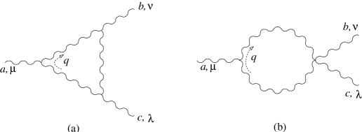
Figure 1: One-loop diagrams, with zero external momenta, which determine the one-loop correction to the CS coefficient.

With the diagrammatic representation of the CS coefficient in the axial gauge (see Eq. (10)), let us note that the one loop correction can be obtained from the two diagrams in Fig. 1. The tree level propagator, with a general gauge fixing parameter, has the form

$$D^{(0)ab}_{\mu\nu}(q) = {\delta^{ab}\over q^{2}-m^{2}+i\epsilon}\left[\eta_{\mu\nu}-{q_{\mu}n_{\nu}+q_{\nu}n_{\mu}\over(n\cdot q)}+{q_{\mu}q_{\nu}n^{2}\over(n\cdot q)^{2}}+im\epsilon_{\mu\nu\lambda}{n^{\lambda}\over(n\cdot q)}\right]$$ (12)

$$+\,\xi\,{p_{\mu}p_{\nu}\over(n\cdot p)^{2}}$$

The propagator in the axial gauge, is then easily obtained by setting $\xi=0$, when it is transverse to $n^{\mu}$ (for an alternative method which involves the use of a Lagrangian multiplier field, see ref. [5]). With this, as well as the interaction vertices derived from Eq. (1), the evaluation of the diagrams in Fig. 1 is straightforward, but tedious (with arbitrary $n^{\mu}$) and shows that, when contracted with $\epsilon_{\mu\nu\lambda}$, the second graph vanishes, while the first graph gives a non zero contribution. Explicitly,

$$I^{abc(1)}_{(a)}=f^{abc}\,{g^{3}\over 4\pi}\,6N,\qquad\qquad{I}^{abc(1)}_{(b)}=0$$ (13)

The one-loop correction to the CS coefficient now follows from Eqs. (10) and (13) to be

$$\Pi_{2}^{(1)}(0)={g^{2}\over 4\pi m}\,N$$ (14)

This is gauge independent (independent of $n^{\mu}$) as claimed and, by the use of relation (11), leads immediately to Eq. (2). Eq. (2), of course, had been derived earlier in the Landau gauge [13], and the present derivation shows that it holds true in the whole class of infrared safe gauges leading to the expectation that ${4\pi m\over g^{2}}$ must represent a physical quantity, as we have argued above.

We would next try to show that the CS coefficient, in the axial gauge, does not receive any further quantum correction from higher loops. To this end, we will use the BRST identities in this gauge, namely, Eq. (9) (which, we would like to emphasize, follows from Eq. (8) with the assumption of analyticity). To simplify our proof, we will use a compact notation, where we treat the amplitudes as matrices (in the Lorentz and internal symmetry space). Thus, we define $\Pi$, $D$, $\Gamma^{\lambda}$ and $\Gamma^{\nu\lambda}$ respectively as the complete two point function, the propagator, the three point and the four point vertex functions. In this notation, then, we have

$$\Pi D=-1$$ (15)

and, furthermore, it is straightforward to see, from Eq. (9), that with the external momentum associated with the index $\lambda$ vanishing, we can write

$$\Gamma^{\lambda} = ig\,\partial^{\lambda}\Pi$$

$${\rm or,}\;\;\;D\Gamma^{\lambda}D = ig\,D(\partial^{\lambda}\Pi)D=ig\,\partial^{\lambda}D$$ (16)

Here and in what follows, $\partial^{\lambda}$ represents the derivative with respect to the appropriate momentum and we have ignored writing out explicitly the internal symmetry factors for simplicity. (Namely, the internal symmetry factors simply come out of the integral and are not relevant to our proof, as will become evident shortly.) There are two classes of diagrams (shown in Figs 2 and 3) which can contribute to higher order corrections of the CS coefficient. Using relations (15)-(16), which hold to any order in perturbation theory, it is now straightforward to show that higher loop corrections (beyond one loop) to the CS coefficient, coming from one particular class of diagrams, vanish.

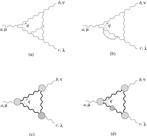
Figure 2: Examples of two-loop diagrams [(a),(b)] which contribute to the three gluon amplitudes [(c),(d)]. Graphs obtained by cyclic permutations of the external gluons are understood to be included.

Let us consider the diagrams in Figs. 2c and 2d, where all external momenta vanish. Here, the hatched vertices and the bold internal lines represent respectively the three point vertices and the propagators which include all the corrections up to $n$-loop order, with $n=0,1,2,\cdots$. The cross-hatched vertex includes all the correction up to $(n+1)$-loop order starting from one-loop (namely, it does not contain the tree level term), while the cross-hatched loop in the internal propagator stands for the self-energy, which includes all the corrections up to $(n+1)$-loop order. We will put an overline on these two factors just to emphasize this aspect, namely, that they do not contain the tree level contribution. By definition, therefore, the diagrams in Figs. 2c and 2d give contributions at two loops and higher. Furthermore, from the definition given above, we can write, with the notation described earlier,

$$\overline{\Gamma}^{\lambda}=ig\,\partial^{\lambda}\overline{\Pi}$$ (17)

The contributions from these diagrams would yield a part of the $(n+2)$ loop corrections to the CS coefficient. Contracting the three point amplitudes in Figs. 2c and 2d with $\epsilon_{\mu\nu\lambda}$, we obtain,

$$I^{(n+2)}_{(2c)+(2d)} = {\rm Tr}\int d^{3}q\,\epsilon_{\mu\nu\lambda}\left[\left(D\Gamma^{\mu}D\Gamma^{\nu}D\left(\overline{\Gamma}^{\lambda}+\Gamma^{\lambda}D\overline{\Pi}\right)\right)^{(n+1)}+{\rm cyclic}\right]$$ (18)

$$= -i\,g^{3}\,{\rm Tr}\int d^{3}q\,\epsilon_{\mu\nu\lambda}\left[\left(\partial^{\mu}D\partial^{\nu}\Pi\left(D\partial^{\lambda}\overline{\Pi}+\partial^{\lambda}D\overline{\Pi}\right)\right)^{(n+1)}+{\rm cyclic}\right]$$

$$= -i\,g^{3}\,{\rm Tr}\int d^{3}q\,\epsilon_{\mu\nu\lambda}\left[\partial^{\lambda}\left(\partial^{\mu}D\partial^{\nu}\Pi D\overline{\Pi}\right)^{(n+1)}+{\rm cyclic}\right]=0$$

for all $n=0,1,2,\cdots$, where the superscript, $(n+1)$, stands for the order of the terms in the expression. Here, “Tr” denotes trace over the matrix indices in the Lorentz space and we have used the identities in Eqs. (15),(16) and (17) in deriving Eq. (18). (There are also matrix indices associated with the internal symmetry space which are not traced, but they are not relevant for our argument as is evident). We note that, because of the epsilon tensor, the factor inside the divergence picks out only the parity violating terms of the amplitude, which converge sufficiently rapidly to zero as $q\rightarrow\infty$. This shows that all the higher loop corrections (two loop and above), to the CS coefficient, coming from this class of diagrams vanish.

There is the second class of diagrams, shown in Fig. 3c, which can also contribute to the CS coefficient. From the identities in Eq. (9), we can express the four point vertex, with two external momenta vanishing, in terms of the three point vertex with one external momentum vanishing in a compact form as (all the momenta are incoming)

$$\Gamma^{\nu\lambda}(0,0,;q,-q)=ig\left[\frac{\partial}{\partial q_{\lambda}}\Gamma^{\nu}(q^{\prime}-q;q,-q^{\prime})\right]_{q^{\prime}=q}\equiv ig\,\partial^{\lambda}\Gamma^{\nu}$$ (19)

where again, we have suppressed the internal indices and we follow the convention that the momenta associated with the indices $\nu,\lambda$ of the four point vertex as well as that associated with the index $\nu$ of the three point vertex vanish. Written out explicitly, the right hand side of Eq. (19) would involve two terms with different distributions of the internal indices, but, as we have emphasized earlier, the internal symmetry factors are not very relevant to the proof of our result.

With these, let us look at the class of graphs in Fig. 3c, with all external momenta vanishing. As opposed to the diagrams in Fig. 2c and 2d, here all the vertices and the propagators include corrections to all orders (namely, they are the full vertices and propagators of the theory). With the use of Eqs. (16) and (19), the contraction of $\epsilon_{\mu\nu\lambda}$ with the amplitude in Fig. 3c yields

$$I_{(3c)} = {\rm Tr}\int d^{3}q\,\epsilon_{\mu\nu\lambda}D\Gamma^{\mu}D\Gamma^{\nu\lambda}=-g^{2}\,{\rm Tr}\int d^{3}q\,\epsilon_{\mu\nu\lambda}\,\partial^{\mu}D\partial^{\lambda}\Gamma^{\nu}$$ (20)

$$= -g^{2}\,{\rm Tr}\int d^{3}q\,\partial^{\mu}\left(\epsilon_{\mu\nu\lambda}D\partial^{\lambda}\Gamma^{\nu}\right)=0$$

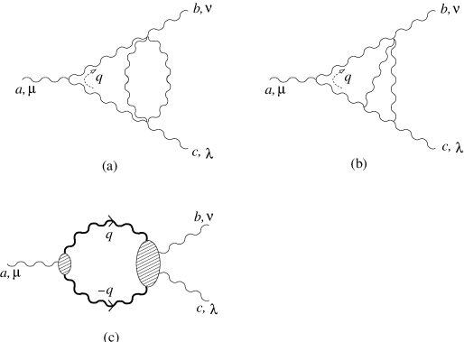
Figure 3: Examples of two-loop Feynman diagrams [(a),(b)] which contribute to the class of graphs (c).

Once again, the integrand in Eq. (20) is sufficiently convergent (because it involves only the parity violating parts of the amplitude) so that the integral vanishes. We have, of course, already seen explicitly, at the one loop level (in Eq. (13)), that this diagram gives a vanishing contribution to the CS coefficient. Eq. (20) shows that this class of diagrams do not contribute to the CS coefficient at all.

Since these are all the diagrams that can contribute to the higher loop corrections of the CS coefficient, we have shown that, in a Yang-Mills-Chern-Simons theory, the CS coefficient, in the axial gauge, does not receive any correction beyond one loop order. In other words, much like the proof in the Abelian theory [3], we have used the non-Abelian Ward identities in the axial gauge, together with the analyticity of the amplitudes in momentum space, to show that the CS coefficient has no quantum correction beyond one-loop in this gauge. In theories where these assumptions are valid, we will expect our proof to hold true. On the other hand, if either of these assumptions is violated, the proof is expected to break down, as would be the case, for example, at finite temperature.

Let us note that, in view of relation (11), this result also means that ${4\pi m\over g^{2}}$ has no correction beyond one loop in this gauge. On the other hand, as we have argued, this is a physical quantity and, therefore, this result must hold true in any other infrared safe gauge such as the Landau gauge and, consequently, Eq. (2) must be exact in such a theory in any infrared safe gauge. We know, however, that, in other non-axial type gauges, such as the Landau gauge, the wave function and the coupling constant renormalizations are not related in a simple manner as in Eq. (5). Consequently, it follows that, in other gauges, the CS coefficient itself will receive higher loop corrections. But these higher loop corrections must be related to the wave function and the vertex renormalizations of the gluon field in such a way that ${4\pi m\over g^{2}}$ has vanishing contribution beyond one loop.

Such a result has, of course, been expected and predicted. In fact, there is a plausibility argument for this, based on large gauge invariance in the following way [7, 13]. The only dimensionless ratio in this theory is ${g^{2}\over 4\pi m}$ ($4\pi$ is a normalization) and can be used as a perturbative expansion parameter. With this, we can write,

$$\left({4\pi m\over g^{2}}\right)_{\rm ren}={4\pi m\over g^{2}}\sum_{n=0}^{\infty}a_{n}(N)\left({g^{2}\over 4\pi m}\right)^{n}$$ (21)

with $a_{0}(N)=1$ and, as we have seen, $a_{1}(N)=N$. On the other hand, the invariance of the Chern-Simons term under large gauge transformations requires that the ratio ${4\pi m\over g^{2}}$ be quantized, both in the bare as well as in the renormalized theory (they don’t have to be the same positive integer). Clearly, this is possible for arbitrary integers and color factors, only if the series, on the right hand side of Eq. (21), terminates after the second term. Our proof explicitly verifies that this expectation is, indeed, justified. However, it is important to recognize that our proof uses constraints coming only from the behavior under small gauge transformations (and, of course, analyticity), much like the proof in the Abelian case.

To summarize, we have shown, using the BRST identities as well as the analyticity of amplitudes, that the CS coefficient does not receive any correction beyond one loop in the axial gauge. We have verified this behavior by an explicit calculation, which shows that all the two loop contributions to the CS coefficient do indeed add up to zero in this gauge. This allows us to conclude that the ratio ${4\pi m\over g^{2}}$ is not renormalized beyond one loop in any infrared safe gauge. For lack of space, we have only sketched our proof and announced various results. The details of the calculation with many other aspects of this problem will be published separately [22].

We would like to thank Gerald Dunne and Roman Paunov for some useful discussions. This work was supported in part by U.S. Dept. Energy Grant DE-FG 02-91ER40685, NSF-INT-9602559 as well as by CNPq, Brazil.

References

- [1] S. S. Chern and J. Simons, Ann. Math. 99 (1974) 48–69.
- [2] S. Deser, R. Jackiw and S. Templeton, Phys. Rev. Lett. 48(1982) 975; Ann. Phys. 140 (1982) 372.
- [3] S. Coleman and B. Hill, Phys. Lett. B159 (1985) 184.
- [4] G. Semenoff, P. Sodano and Y.-S. Wu, em Phys. Rev. Lett. 62 (1989) 715.
- [5] A. Das, Finite Temperature Field Theory, World Scientific (1997).
- [6] F. T. Brandt, A. Das, J. Frenkel, and K. Rao, hep-th/0009031 (to appear in Phys. Lett. B).
- [7] Y.-C. Kao and M. Suzuki, Phys. Rev. D31 (1985) 2137.
- [8] M. D. Bernstein and T. Lee, Phys. Rev. D32 (1985) 1020.
- [9] M. Sakamoto and H. Yamashita, Phys. Lett. B476 (2000) 427, hep-th/9910200.
- [10] N. Seiberg, Phys. Lett. B318 (1993) 469–475, hep-ph/9309335.
- [11] R. Jackiw and S. Templeton, Phys. Rev. D23 (1981) 2291.
- [12] A. N. Redlich, Phys. Rev. D29 (1984) 2366.
- [13] R. D. Pisarski and S. Rao, Phys. Rev. D32 (1985) 2081.
- [14] K. S. Babu, A. Das, and P. Panigrahi, Phys. Rev. D36 (1987) 3725.
- [15] G. V. Dunne, Les Houches (1998), hep-th/9902115.
-
[16]
E. Witten, Comm. Math. Phys. 121 (1989) 351;
S. Elitzur, G. Moore, A. Schwimmer and N. Seiberg, Nucl. Phys. 326 (1989) 108;
M. Bos and V. P. Nair, Int. J. Mod. Phys. A5 (1990) 959. - [17] A. Polyakov, Fields, Strings and Critical Phenomena, Les Houches, eds. E. Brézin and J. Zinn-Justin (1988).
- [18] K. Gawedzki and A. Kupiainen, Nucl. Phys. B320 (1989) 625.
-
[19]
W. Kummer, Acta Phys. Austriaca 14 (1961)
149; ibid 41 (1975) 315;
R. L. Arnowitt and S. Fickler, Phys. Rev. 127 (1962) 1821;
J. Frenkel, Phys. Rev. D13 (1976) 2325;
G. Leibbrandt, Rev. Mod. Phys. 59 (1987) 1067. - [20] S. Mandelstam, Nucl. Phys. 213 (1983) 149.
- [21] N. K. Nielsen, Nucl. Phys. B101 (1975) 173.
- [22] F. T. Brandt, A. Das and J. Frenkel, in preparation.