UNITU–THEP–16/2000

Abelian and center gauges in continuum Yang-Mills-Theory

H. Reinhardt and T. Tok

Institut für Theoretische Physik, Universität Tübingen
Auf der Morgenstelle 14, D-72076 Tübingen, Germany

Abelian and center gauges are considered in continuum Yang-Mills theory in order to detect the magnetic monopole and center vortex content of gauge field configurations. Specifically we examine the Laplacian Abelian and center gauges, which are free of Gribov copies, as well as the center gauge analog of the (Abelian) Polyakov gauge. In particular, we study meron, instanton and instanton-anti-instanton field configurations in these gauges and determine their monopole and vortex content. While a single instanton does not give rise to a center vortex, we find center vortices for merons. Furthermore we provide evidence, that merons can be interpreted as intersection points of center vortices. For the instanton-anti-instanton pair, we find a center vortex enclosing their centers, which carries two monopole loops.

PACS: 11.15.-q, 12.38.Aw

Keywords: Yang-Mills theory, center vortices, maximal center gauge, Laplacian center gauge

1 Introduction

At present there are two popular confinement mechanisms: the dual Meissner effect [2, 3, 4], which is based on a condensation of magnetic monopoles in the QCD vacuum and the vortex condensation picture [5, 6]. Both pictures were proposed long time ago, but only in recent years mounting evidence for the realization of these pictures has been accumulated in lattice calculations. The two pictures of confinement show up in specific partial gauge fixings.

Magnetic monopoles arise as gauge artifacts in the so-called Abelian gauges proposed by ’t Hooft [7], where the Cartan subgroup $H$ of the gauge group $G$ is left untouched, fixing only the coset $G/H$. To be more precise the magnetic monopoles explicitly show up only after the so-called Abelian projection, which consists in throwing away the “charged” part of the gauge field after implementing the Abelian gauge. Magnetic monopoles appear at those isolated points in space, where the residual gauge freedom is larger than the Abelian subgroup.

Since the magnetic monopoles arise as gauge artifacts, their occurrence and properties depend on the specific form of the Abelian gauge used. For example, monopole dominance in the string tension [8, 9, 10] is found in maximally Abelian gauge, but not in Polyakov gauge [11] (in Polyakov gauge there is, however, an exact Abelian dominance in the temporal string tension). However, in all forms of the Abelian gauges considered monopole condensation occurs in the confinement phase and is absent in the de-confinement phase [12].

The vortex picture of confinement, which received rather little attention after some early efforts following its inception has recently received strong support from lattice calculations performed in the so-called maximum center gauge [13, 14], where one fixes only the coset $G/Z$ but leaves the center $Z$ of the gauge group $G$ unfixed. Subsequent center projection, which consists in replacing each link by its closest center element allows the identification of the center vortex content of the gauge fields. Lattice calculations show, that the vortex content detected after center projection produces virtually the full string tension, while the string tension disappears, if the center vortices are removed from the lattice ensemble [13, 16]. This fact has been referred to as center dominance. Center dominance persists at finite temperature [17, 18] for both the $q-\bar{q}$ potential (Polyakov loop correlator) as well as for the spatial string tension. The vortices have also been shown to condense in the confinement phase [19]. Furthermore in the gauge field ensemble devoid of center vortices chiral symmetry breaking disappears and all field configurations belong to the topologically trivial sector [16].

Unfortunately, both gauge fixing procedures, the maximally Abelian gauge and the maximum center gauge, suffer from the Gribov problem [20], both on the lattice as well as in the continuum [21].

To circumvent the Gribov problem, the Laplacian gauge [22], the Laplacian Abelian gauge [23] and the Laplacian center gauge [24, 25] have been introduced. In the latter two gauges, which are free of Gribov copies, one uses eigenvectors of the covariant Laplace operator in the adjoint representation to fix the gauge. These eigenvectors transform homogeneously under gauge rotations. In the Laplacian Abelian gauge fixing one exploits the gauge freedom to rotate the lowest eigenvector of the covariant Laplacian into the Cartan subalgebra. In the Laplacian center gauge, one uses the residual Abelian gauge freedom, which remains after Laplacian Abelian gauge fixing to rotate the next to lowest eigenvector into the plane spanned by the first and third axes in color space (for gauge group $SU(2)$). The Laplacian center gauge fixing has the advantage, that the magnetic monopoles lie on the vortices by construction.

In this paper we consider various types of Abelian and center gauges in continuum Yang-Mills theory and study in these gauges field configurations which are considered to be relevant in the infrared sector of QCD like center vortices, instantons and merons. Center vortices can give an appealing explanation of confinement (see e.g. ref. [18]). It is the general consense that instantons have little to do with confinement but offer an explanation of spontaneous breaking of chiral symmetry [26, 27]. Merons can be considered as “half of an instanton with zero radius” and we will provide evidence that they can be regarded as intersection points of center vortices.

The advantage of the Abelian and center gauges is that they provide a convenient tool to detect the monopole and vortex content of a field configuration.

Previously the monopole content of instantons has been considered in the Polyakov gauge and maximally Abelian gauge [28, 29, 30, 31]. In maximally Abelian gauge a monopole trajectory was found to pass through the center of the instanton in ref. [28], while an infinitesimal monopole loop around the center of the instanton was found in [30]. These results are consistent with the findings of [32] where an instanton on an $S^{4}$-space-time manifold has been considered and a monopole loop degenerate to a point was found in Laplacian Abelian gauge. Only for a special choice of the instanton scale one can find a monopole loop of finite size [32]. In Polyakov gauge [33] a static monopole trajectory passes through the center of the instanton [34]. In this gauge the Pontryagin index can be entirely expressed in terms of magnetic monopole charges [35, 36, 37, 38].

The vortex content of instanton field configurations has been less understood. The first investigations in this direction have been reported in ref. [24, 25] where a cooled two instanton configuration and a cooled caloron configuration have been considered in the Laplacian center gauge on the lattice. In the former case a vortex sheet was found connecting the positions of the two instantons. In the case of the caloron which can be interpreted as a monopole-anti-monopole pair the vortex sheet runs through the positions of monopole and anti-monopole, which is expected since in the Laplacian center gauge by construction the monopoles are sitting on the vortex sheets. One should, however, keep in mind that the lattice result cannot be straightforwardly transferred to the continuum. Due to the periodic boundary conditions a localized configuration on the lattice corresponds to an array of such configurations in the continuum. In addition the detection of topological charge on the lattice is problematic on its own.

In this paper we study various field configurations like vortices, instantons and merons in the continuum analog of the Laplacian center gauge. The organization of the paper is as follows: In section 2 we define Abelian and center gauges by means of one and two, respectively, color fields transforming homogeneously under gauge transformations. In section 3 we discuss the Laplacian Abelian and center gauges in continuum Yang-Mills-theory and provide examples for field configurations giving rise to magnetic monopoles and center vortices after Laplacian Abelian and center gauge fixing, respectively. In section 4 merons, instantons and instanton-anti-instanton pairs are considered in the Laplacian Abelian and center gauges. We also provide evidence that merons can be interpreted as vortex intersection points. Some concluding remarks are given in section 5.

2 Abelian and center gauges

In the following we consider Abelian and center gauges from a general point of view.

Since the center $Z$ of a group $G$ belongs to its Cartan subgroup $H$ (center) gauge fixing can be formed in two steps: First one fixes the coset $G/H$ leaving the Cartan subgroup $H$ unfixed, which is referred to as Abelian gauge fixing. Secondly one fixes the coset $H/Z$ leaving the center unfixed, which is referred to as center gauge fixing. In this paper we will mainly concentrate on $G=SU(2)$ and $H=U(1)$. For a recent generalization of the Laplacian center gauge fixing to the gauge group $SU(N)$ see ref. [39].

2.1 Abelian gauge

In this section we will shortly discuss Abelian gauges. It is a gauge fixing procedure which fixes the gauge group $G$ up to its Cartan subgroup $H$. For the Abelian gauge fixing one considers a Lie algebra valued field $\psi_{1}$ in the adjoint representation transforming homogeneously under gauge transformations. In the following we will refer to such a field as “Higgs field”. This field can be given as the solution to some covariant field equation or as the extremum of some gauge independent functional. Examples will be given in section 3.

Now we fix the gauge by demanding that $\psi_{1}(x)$ points in the $3$-direction of color space for every $x\in M$, $M$ being the space-time manifold, i.e. we are searching for a gauge transformation $V$ such that

$$V(x)^{-1}\psi_{1}(x)V(x)=h(x)\sigma_{3}\,,\quad h(x)\geq 0\,.$$ (2.1)

For $\psi_{1}(x)\neq 0$ the transformation matrix $V(x)$ is defined up to a residual $U(1)$ gauge transformation $V(x)\rightarrow V(x)\exp(\alpha(x)\sigma_{3}/(2i))$. However, if $\psi_{1}(x)=0$, then $V(x)$ is arbitrary and the residual gauge freedom is enlarged to the full gauge group $SU(2)$. At such points the function $V(x)$ will in general become singular. This leads us to the definition of the Abelian defect manifold

$${\cal D}_{A}:=\left\{x\in M;\psi_{1}(x)=0\right\}\,.$$ (2.2)

Any connected one-dimensional subset of ${\cal D}_{A}$ can be identified with a magnetic monopole loop with respect to the residual $U(1)$ gauge freedom. This is because for $G=SU(2)$ the condition $\psi_{1}(x)=\psi_{1}^{a}\sigma_{a}=0$ implies 3 equations $\psi_{1}^{a=1,2,3}(x)=0$ which generically define a one-dimensional manifold in $D=4$, the monopole trajectory. On ${\cal D}_{A}^{c}:=M\setminus{\cal D}_{A}$ we define the Abelian magnetic gauge potential [7, 40]

$$A_{{\mathrm{m}ag}}:=\mbox{Tr}(V^{-1}{\mbox{d}}VT_{3})\,,\quad T_{3}=\sigma_{3}/(2i)$$ (2.3)

and find for its field strength

$$F_{{\mathrm{m}ag}}:={\mbox{d}}A_{{\mathrm{m}ag}}=-\mbox{Tr}(V^{-1}{\mbox{d}}V\wedge V^{-1}{\mbox{d}}VT_{3})\,.$$ (2.4)

The field strength $F_{{\mathrm{m}ag}}$ does not depend on the special choice of $V$, which is defined only up to a $U(1)$ gauge transformation. Surrounding a monopole by a surface ${\cal S}$ and integrating $F_{{\mathrm{m}ag}}$ over ${\cal S}$ results in the magnetic charge $q$ inside ${\cal S}$:

$$q=\frac{1}{2\pi}\int_{\cal S}F_{{\mathrm{m}ag}}\,.$$ (2.5)

Geometrically the monopole charge $q$ is nothing but the winding number of the map $\hat{\psi}_{1}:{\cal S}\rightarrow SU(2)/U(1)\equiv S^{2}$ [41]. The image $S^{2}$ is given by the unit color vectors in the Lie algebra $su(2)$, obtained by normalizing the Higgs field: $\hat{\psi}_{1}(x)=\psi_{1}(x)/|\psi_{1}(x)|$. If $q\neq 0$ it follows that $V$ cannot be chosen smoothly on ${\cal S}$. $V$ has to be singular on a Dirac string emanating from the monopole inside ${\cal S}$, and the Dirac string punctures ${\cal S}$. The explicit location of the Dirac strings is arbitrary — the only requirement is that the total charge of a connected monopole-Dirac-string-network has to vanish. Everywhere outside the Dirac strings and the monopoles we can choose $V$ smoothly.

Near its zeros the Higgs field of a charge one monopole looks in an appropriate choice of coordinates like a hedgehog:

$$\psi_{1}(x)=\sum_{i=1}^{3}x^{i}\sigma_{i}\,.$$ (2.6)

as follows by a Taylor expansion of $\psi_{1}(x)$ around its zeros. The hedgehog is diagonalized by the matrix $V=\exp(\vartheta\sigma_{\varphi}/(2i))$ for which the Abelian part of the induced gauge field $V^{-1}{\mbox{d}}V$ develops a Dirac monopole:

$$V^{-1}{\mbox{d}}V = \frac{\sigma_{\varphi}}{2i}{\mbox{d}}\vartheta-\left(\sin\vartheta\cos\varphi\frac{\sigma_{1}}{2i}+\sin\vartheta\sin\varphi\frac{\sigma_{2}}{2i}\right){\mbox{d}}\varphi-(1-\cos\vartheta)\frac{\sigma_{3}}{2i}{\mbox{d}}\varphi\,,$$ (2.7)

$$A_{{\mathrm{m}ag}} = \frac{1}{2}(1-\cos\vartheta){\mbox{d}}\varphi\,,$$ (2.8)

where we used spherical coordinates in ${\mathbb{R}}^{3}$. Its magnetic charge is $q=1$ which is equal to the winding number of the normalized Higgs field $\hat{\psi}=\hat{x}$ around $x=0$.

From a geometrical point of view the set of all matrices $V(x)$, $x\in{\cal D}^{c}_{A}$ rotating $\psi_{1}(x)$ into the $\sigma_{3}$ direction defines a principal bundle $P_{A}$ over ${\cal D}^{c}_{A}$. A smooth gauge transformation $V$ is a global section in $P_{A}$. On the other hand, the existence of magnetic monopoles tells us that the bundle $P_{A}$ is not trivial and we have to introduce Dirac strings on which a global section in the bundle is singular.

2.2 Center gauge

In this section we will discuss center gauges fixing the gauge group up to its center. These gauges are extensions of Abelian gauges discussed in the previous section. To this end we consider a second Higgs field $\psi_{2}(x)$ in the adjoint representation. Again it should be given as the solution to some covariant field equation or as the extremum of some gauge independent functional (examples are given in section 3).

After having fixed the gauge group up to its Cartan subgroup, we use the remaining Abelian gauge freedom $g(x)\in H$ to rotate $\psi_{2}(x)$ into the plane spanned by $\sigma_{3}$ and $\sigma_{1}$ in color space:

$$\psi_{2}^{Vg}(x)=g^{-1}V^{-1}(x)\psi_{2}(x)V(x)g = l_{3}(x)\sigma_{3}+l_{1}(x)\sigma_{1},$$ (2.9)

$$l_{1},l_{3}\in{\mathbb{R}}\,,\quad l_{1}(x)\geq 0\,,\quad g\in H\,.$$

Alternatively one can express this condition by saying that the part of the color vector $\psi_{2}(x)^{V}$ perpendicular to the $3$-direction, ${\psi_{2}}_{\perp}$, is rotated into the $1$-direction. As long as $\psi_{1}(x)$ and $\psi_{2}(x)$ are linearly independent the conditions (2.1,2.9) fix $V(x)g(x)$ up to a factor $\pm 1$, i.e. up to the center of $SU(2)$. But, if $\psi_{1}(x)$ and $\psi_{2}(x)$ are linearly dependent, then the residual gauge freedom is enlarged. At such points the gauge transformation $Vg$ will in general be singular. This brings us to the definition of the center defect manifold

$${\cal D}_{C}:=\left\{x\in M;\psi_{1}(x)\,\mbox{and}\,\psi_{2}(x)\,\mbox{are linearly dependent}\right\}\,.$$ (2.10)

A connected two-dimensional subset of ${\cal D}_{C}$ will be called vortex. There are two conditions to be fulfilled for the linear dependence of the color vectors $\psi_{1}(x)$ and $\psi_{2}(x)$. Therefore the vortices have co-dimension 2, i.e. they are one-dimensional lines in $D=3$ and two-dimensional sheets in $D=4$. By definition ${\cal D}_{A}\subset{\cal D}_{C}$ (if $\psi_{1}(x)=0$, then $\psi_{1}(x)$ and $\psi_{2}(x)$ are obviously linearly dependent). Therefore the monopoles identified in the Abelian gauge lie on top of the vortices identified in the center gauge.

We should emphasize that the vortices identified in the center gauge in the way described above correspond to the ideal center vortices obtained in the maximal center gauge after center projection. Like in the latter case the vortices identified in the above described center gauge carry flux which is not identical to the flux carried by the original gauge field.

As an illustrative example consider the following Higgs fields in $D=3$

$$\psi_{1}=\sigma_{3}\,,\,\psi_{2}(\rho,\varphi,z)=\sigma_{3}+\rho(\cos(n\varphi)\sigma_{1}+\sin(n\varphi)\sigma_{2})\,,\quad n\in{\mathbb{Z}}\,,$$ (2.11)

where we used polar coordinates. The gauge transformation which brings the field into the center gauge ($g^{-1}\psi_{2}g=\sigma_{3}+\rho\sigma_{1}$) reads

$$g(\rho,\varphi,z)=\pm\exp(n\varphi T_{3})\,,\quad T_{3}=\sigma_{3}/(2i)\,.$$ (2.12)

For even $n$ this gauge transformation is smooth everywhere except on the $z$-axis ($\rho=0$), where $\varphi$ is ill-defined, see figure 2. However, for odd $n$ the gauge transformation $g$ becomes double-valued, i.e. we have to introduce a cut (emanating from the $z$-axis) on which $g$ jumps by $-1$, see figure 2. The line singularity on the $z$-axis represents a Dirac string for even $n$ and a center vortex for odd $n$.

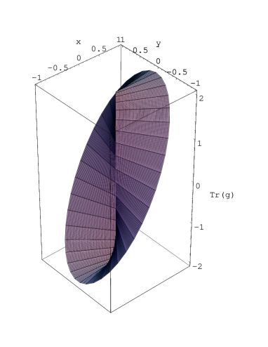
Figure 1: Plot of the trace of the gauge transformation $g$, see equ. (2.12), for $n=2$ and positive sign. There is a Dirac string at $x=y=0$. The gauge transformation can be chosen smoothly everywhere except on the Dirac string.

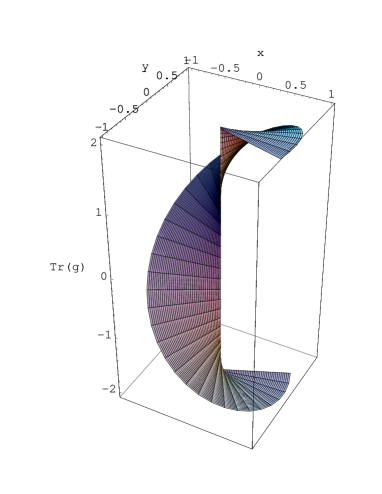
Figure 2: Plot of the trace of the gauge transformation $g$, see equ. (2.12), with $n=1$ and positive sign. There is a center vortex at $x=y=0$. The gauge transformation $g$ has to jump by $-1$ on a cut emanating from the vortex. At the vortex the gauge transformation $g$ is obviously singular.

On the $z$-axis $\psi_{2}=\sigma_{3}$, see (2.11), and hence $\psi_{2}$ is here parallel to $\psi_{1}$. According to the previously given definition of center vortices in the center gauge the $z$-axis hosts a center vortex. Indeed for odd $n$ the line singularity in $g$ on the $z$-axis induces a center vortex in the center gauge transformed potential $A^{g}=g^{-1}Ag+g^{-1}{\mbox{d}}g$. However for even $n$ the line singularity in the gauge transformation $g$ on the $z$-axis gives rise to a Dirac string in $g^{-1}{\mbox{d}}g$. To see this we calculate the magnetic flux carried by $A_{{\mathrm{m}ag}}$ (2.3) through an infinitesimal loop ${\cal C}$ encircling the $z$-axis. Using (2.12) we find

$$\Phi = \frac{1}{2\pi}\oint_{\cal C}A_{{\mathrm{m}ag}}=\frac{1}{2\pi}\oint_{\cal C}\mbox{Tr}((Vg)^{-1}{\mbox{d}}(Vg)T_{3})$$ (2.13)

$$= \frac{1}{2\pi}\oint_{\cal C}\mbox{Tr}(g^{-1}V^{-1}({\mbox{d}}Vg+V{\mbox{d}}g)T_{3})=\frac{1}{2\pi}\oint_{\cal C}\mbox{Tr}(g^{-1}{\mbox{d}}gT_{3})$$

$$= \frac{1}{2\pi}\oint_{\cal C}\mbox{Tr}((nT_{3}{\mbox{d}}\varphi)T_{3})=-\frac{1}{2\pi}\oint_{\cal C}n/2{\mbox{d}}\varphi$$

$$= -n/2\,.$$

The term with $V^{-1}{\mbox{d}}V$ in the second line vanishes in the limit of an infinitesimal loop ${\cal C}$, because $V$ can be chosen smoothly on the vortex (away from monopoles). For $n$ even (odd) we find integer (half-integer) flux carried by a Dirac sheet (center vortex sheet). Furthermore, the Wilson loop ${\cal P}\exp(-\oint_{\cal C}(Vg)^{-1}{\mbox{d}}(Vg))$ becomes $-1$ (in general a non-trivial center element) for center vortices and $+1$ for Dirac sheets. Thus a Dirac sheet is indeed not seen, i.e. unobservable by the Wilson loop, as it should since it is a gauge artifact.

From the above considerations it is clear that we can interpret Dirac sheets as two center vortex sheets on top of each other. Then it is obvious that at a monopole there are at least two center vortices coming in.

The important lessen from the study of the above example is that the procedure of identifying center vortices in the center gauge catches not just center vortices but also Dirac strings.

However, the generic case is the occurrence of center vortices. To show this let us consider a sheet singularity ${\cal V}\subset{\cal D}_{C}$ and a point $x_{0}$ on it, i.e. $\psi_{1}(x_{0})\sim\psi_{2}(x_{0})$. Further we demand $\psi_{1}(x_{0})\neq 0$ and $\psi_{2}(x_{0})\neq 0$. We choose a 2-dimensional face ${\cal F}$ through $x_{0}$ which is vertical to ${\cal V}$, i.e. ${\cal F}$ traverses ${\cal V}$ only at $x_{0}$. We make a gauge transformation $V$ which rotates $\psi_{1}$ into the $\sigma_{3}$ direction. This gauge transformation can be chosen smoothly in a neighborhood of $x_{0}$, because $\psi_{1}(x_{0})\neq 0$. We consider the gauge transformed normalized field $\hat{\psi}_{2}^{V}$ on ${\cal F}$. The field $\hat{\psi}_{2}^{V}$ takes values in the unit sphere in $su(2)\equiv{\mathbb{R}}^{3}$, i.e. on a two-sphere $S^{2}$. Hence it makes sense to calculate the functional determinant of the map $\hat{\psi}_{2}:{\cal F}\to S^{2}$ at the point $x_{0}$. Generically this determinant is nonzero. For non-vanishing functional determinant, using Taylor expansion, we can introduce coordinates $x^{1},x^{2}$ on ${\cal F}$ such that in an infinitesimal neighborhood of $x_{0}$ the field $\hat{\psi}_{2}^{V}(x)$ looks like

$$\hat{\psi}_{2}^{V}(x)=\pm\sigma_{3}+(x-x_{0})^{1}\sigma_{1}+(x-x_{0})^{2}\sigma_{2}\,.$$

Changing into polar coordinates on ${\cal F}$ the fields $\psi_{1}^{V},\psi_{2}^{V}$ have the form (2.11) with $n=1$. Completing the center gauge fixing results obviously in a center vortex at $x_{0}$.

We can again visualize the gauge fixing geometrically in a bundle picture. Appending to each $x\in{\cal D}_{C}^{c}=M\setminus{\cal D}_{C}$ the two matrices $\{V(x)g(x),-V(x)g(x)\}$, which fulfill (2.1,2.9) we get a principal bundle $P_{C}$ with structure group ${\mathbb{Z}}_{2}$. The bundle $P_{C}$ is a twofold covering manifold of ${\cal D}_{C}^{c}$. In analogy to complex function theory of a double-valued function (e.g. $\sqrt{z}$) we may look at $P_{C}$ as the Riemann surface of a double-valued function. The vortices can be identified as branching points. This gives us the opportunity to classify the line (surface) singularities in $D=3$ ($D=4)$. We consider a closed loop surrounding the singularity and lift this loop into the covering manifold $P_{C}$. There are two classes of lifted loops - they can be closed (remain on the same sheet of the Riemann surface) or open (change the sheet of the Riemann surface). If the lifted loop is closed, the singularity represents a Dirac string. If the lifted loop is open (i.e. it jumps by $-1$ at the endpoint), the singularity represents a center vortex, compare also with figures 2 and 2.

We are interested in a globally well defined gauge transformation $V$ on ${\cal D}_{C}^{c}$. But for this we have to introduce cuts emanating from the center vortices. At these cuts the gauge transformation $V$ jumps by the center element $-1$. If one would work with gauge group $SO(3)$ from the very beginning these cuts would be invisible, because $SO(3)\equiv SU(2)/{\mathbb{Z}}_{2}$, i.e. the center is projected out.

From the considerations above we can also conclude that center vortices cannot have a boundary - they have to form closed lines or surfaces. Let us assume there is an end-point of a center vortex. We consider a closed loop ${\cal C}$ around the center vortex near the end-point. Then there exists a surface ${\cal S}$ bounded by ${\cal C}$ such that the center vortex does not intersect ${\cal S}$, see fig. 3. Consider now the double-valued covering of ${\cal S}$ given by the set of matrices $\{V(x)g(x),-V(x)g(x)\}\,,\,x\in{\cal S}$ fulfilling (2.1,2.9). Because ${\cal S}$ is contractible (i.e. $\pi_{1}({\cal S})=\{1\}$) the covering of ${\cal S}$ is topologically given by ${\cal S}\times{\mathbb{Z}}_{2}$. Hence, if we lift the loop ${\cal C}$ into the bundle $P_{C}$ the lifted loop is well defined and has no jumping points. But this contradicts our assumption that there is a center vortex with an end-point.

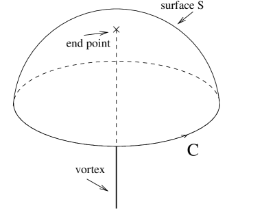
Figure 3: Illustration of the closedness of center vortices.

Especially center vortices cannot end at monopoles, i.e. if there is one center vortex going in, there must be a second center vortex going in the monopole. On the other hand Dirac sheets can be open, i.e. bounded by monopole loops.

3 Specific Abelian and center gauges

Above we have considered Abelian and center gauge fixing from a general point of view using two “Higgs” fields, i.e. colour fields living in the algebra of the gauge group and transforming covariantly (homogeneously) under gauge transformations. Now we will consider specific choices of these Higgs fields. We will start by considering the continuum version of the Laplacian gauge.

3.1 Laplacian Abelian and center gauge

In the Laplacian gauge the Higgs fields $\psi_{1},\psi_{2}$ are identified with the eigenfunctions of the two lowest eigenvalues of the covariant Laplace operator [23, 24, 39]

$$-\hat{\mbox{D}}_{\mu}(A)\hat{\mbox{D}}_{\mu}(A)\psi_{i}=\lambda_{i}\psi_{i}\,,$$ (3.1)

where

$$\hat{\mbox{D}}_{\mu}(A)\psi=[{\mbox{D}}_{\mu}(A),\psi]\,.$$ (3.2)

As the Laplace operator is positive semidefinite all eigenvalues are non-negative, i.e. $\lambda_{i}\geq 0$. The eigenvectors $\psi_{i}(x)$ transform covariantly under gauge transformations and, in principle, we could use any two eigenvectors $\psi_{i},\psi_{k}$ as the Higgs fields for Abelian or center gauge fixing. However, the spirit of the Abelian and center gauge fixing is to extract the infrared degrees of freedom as gauge fixing defects. For this purpose one should use the lowest lying eigenvectors as Higgs fields since they carry the infrared content of a gauge field configuration $A_{\mu}(x)$.

In the following we study the effect of Abelian and center Laplacian gauge fixing for specific field configurations.

3.1.1 Laplacian Abelian gauge

To demonstrate the emergence of magnetic monopoles in the Laplacian Abelian gauge [23] fixing let us consider the following gauge potential

$$A_{i}=0,i=1,2,3\,,\,A_{0}=a(r)\frac{x_{k}}{r}T_{k}\,,\,r^{2}=x_{1}^{2}+x_{2}^{2}+x_{3}^{2}\,,\,a(r)=\sin(\pi r/R)\,,\,T_{k}=\sigma_{k}/(2i)$$ (3.3)

on the space time manifold $D_{3}\times S^{1}$ (three dimensional ball with radius $R$ times circle with circumference $\beta$). As boundary conditions we demand periodicity in time and $\psi_{1}=0$ on the boundary of $D_{3}$, implying there is a magnetic monopole on the boundary of $D_{3}$. The Laplace operator acting on $\psi_{1}=\psi_{1}^{k}\sigma_{k}$ reads

$$-\hat{\mbox{D}}^{2}\psi_{1}=-\left(\partial_{i}\partial_{i}\delta_{kl}+\partial_{0}^{2}\delta_{kl}+2a\frac{x_{j}}{r}\varepsilon_{jkl}\partial_{0}-a^{2}\delta_{kl}+a^{2}\frac{x_{k}x_{l}}{r^{2}}\right)\psi_{1}^{k}\sigma_{l}\,.$$ (3.4)

The ground state wave function is time independent and of hedgehog type, i.e.

$$\psi_{1}^{k}=\frac{x^{k}}{r}b(r)\,.$$ (3.5)

The function $b(r)$ has to fulfill the differential equation

$$r^{2}b^{\prime\prime}+2rb^{\prime}+(\lambda_{1}r^{2}-2)b=0\,,$$ (3.6)

where $\lambda_{1}$ is the non-negative eigenvalue of the ground state of the covariant Laplacian (3.4). The solution to this equation is

$$b(r)=C\frac{1}{\sqrt{\lambda_{1}}r}\left(\frac{\sin(\sqrt{\lambda_{1}}r)}{\sqrt{\lambda_{1}}r}-\cos(\sqrt{\lambda_{1}}r)\right)\,.$$

The minimal eigenvalue $\lambda_{1}$ is defined by the boundary condition $b(R)=0$, i.e. $\lambda_{1}\approx(4.4934/R)^{2}$.

Abelian gauge fixing (2.1) implies here to rotate the color vector defined by the ground state (3.5) of the covariant Laplace operator into the $3$-direction and results in a static monopole line at $r=0$ (cf. equations (2.6,2.8)). With the gauge transformation (2.7) we get a Dirac string on the negative $z$-axis. It connects the location of the magnetic monopole at $r=0$ with the one on the boundary of $D_{3}$.

3.1.2 Laplacian center gauge

As an example we will consider a thick vortex along the $z$-axis in three dimensional space $D_{2}\times S_{1}$ (two dimensional disc with radius $D$ times circle with radius $Z$):

$$A=f(\rho){\mbox{d}}\varphi T_{3}\,,\,f(\rho=0)=0,f(\rho=D)=1\,,$$ (3.7)

where we used cylinder coordinates. The gauge potential is invariant under rotation around the $z$-axis and under translation along the $z$-axis. For the Laplacian center gauge fixing we choose the two “Higgs” fields $\psi_{1,2}$ to be given by the ground state and first excited state, respectively, of the covariant Laplacian. Thereby we impose the boundary conditions that the Higgs fields vanish on the surface of the cylinder(for $\rho=D$) and are periodic in the $z$-direction. The covariant Laplace operator on $\psi_{1,2}=\psi_{1,2}^{k}\sigma_{k}$ reads

$$\hat{\mbox{D}}_{i}\hat{\mbox{D}}_{i}\psi_{1,2} = (\frac{1}{\rho}\partial_{\rho}\rho\partial_{\rho}+\frac{1}{\rho^{2}}\partial_{\varphi}^{2}+\partial_{z}^{2})\psi_{1,2}^{k}\sigma_{k}+\frac{f(\rho)^{2}}{\rho^{2}}\psi_{1,2}^{k}[T_{3},[T_{3},\sigma_{k}]]+$$ (3.9)

$$2\frac{f(\rho)}{\rho^{2}}\partial_{\varphi}\psi_{1,2}^{k}[T_{3},\sigma_{k}].$$

Setting

$$\psi_{1,2}^{c}=\psi_{1,2}^{1}+i\psi_{1,2}^{2}$$ (3.10)

we get the following differential equations:

$$(\frac{1}{\rho}\partial_{\rho}\rho\partial_{\rho}+\frac{1}{\rho^{2}}\partial_{\varphi}^{2}+\partial_{z}^{2})\psi_{1,2}^{3} = -\lambda\psi_{1,2}^{3}$$ (3.11)

$$(\frac{1}{\rho}\partial_{\rho}\rho\partial_{\rho}+\frac{1}{\rho^{2}}\partial_{\varphi}^{2}+\partial_{z}^{2})\psi_{1,2}^{c}-\frac{f(\rho)^{2}}{\rho^{2}}\psi_{1,2}^{c}+2\frac{f(\rho)}{\rho^{2}}i\partial_{\varphi}\psi_{1,2}^{c} = -\lambda\psi_{1,2}^{c}.$$ (3.12)

If we make a separation ansatz for $\psi_{1,2}^{3}$ we get the Bessel differential equation for its $\rho$-dependence. The ground state is then given by $\psi_{1}^{c}=0$ and $\psi_{1}^{3}=J_{0}(\sqrt{\lambda}\rho)$, where $J_{0}$ is the zeroth Bessel function. The minimal eigenvalue $\lambda$ is defined by the boundary condition $J_{0}(\sqrt{\lambda}D)=0$, i.e. $\lambda_{1}\approx(2.4048/D)^{2}$. The first excited state is given by $\psi_{2}^{3}=0$ and $\phi_{2}^{c}=g(\rho)\exp(-i\varphi)$, where $g$ has to fulfill the differential equation

$$\rho^{2}g^{\prime\prime}+\rho g^{\prime}+(\lambda\rho^{2}-(1-f)^{2})g=0.$$ (3.13)

As an example let us take

$$f(\rho)=1-\exp(-\rho/(1-\rho/D)),D=10\,.$$ (3.14)

Figure 4: The vortex profile function f, cp. (3.14).

Figure 5: The function g for the first excited state, cp. (3.13).

The eigenvalue of the first excited state is $\lambda_{2}\approx 0.0835062$ and its wave function has the form $\psi_{2}(\rho,\varphi,z)=g(\rho)(\sigma_{1}\cos\varphi-\sigma_{2}\sin\varphi)$. After center gauge fixing this configuration leads to a center vortex on the $z$-axis, i.e. subsequent Abelian projection (replacing the full gauge potential by its Abelian part) results in a “thin” vortex

$$A_{{\mathrm{m}ag}}={\mbox{d}}\varphi T_{3}\,.$$ (3.15)

Thus in the continuum Abelian projection after Laplacian center gauge fixing converts a thick center vortex into a thin one. This is analogous to what happens in center projection after maximal center gauge fixing on the lattice [15].

3.2 Abelian and center gauges from Wilson lines

Here we consider space-time to be given by a $4$-torus and define fields $\phi_{1}$ and $\phi_{2}$ as path ordered exponentials of the gauge potential around different circumferences of the torus. But first we have to remind some facts about gauge fields on the torus.

We consider the torus as ${\mathbb{R}}^{4}$ modulo a discrete lattice spanned by 4 orthogonal vectors $b_{\mu}$, $\mu=1,\ldots,4$, having lengths $L_{\mu}=|b_{\mu}|$. A gauge potential on the torus ${\mathbb{T}}^{4}$ is then given by a gauge potential on ${\mathbb{R}}^{4}$ fulfilling periodicity properties:

$$A(x+b_{\mu})=U_{\mu}^{-1}(x)A(x)U_{\mu}(x)+U_{\mu}^{-1}(x){\mbox{d}}U_{\mu}(x)\,,$$ (3.16)

where the $U_{\mu}$ are called transition functions and they fulfill the Co-cycle condition:

$$U_{\mu}(x)U_{\nu}(x+b_{\mu})=U_{\nu}(x)U_{\mu}(x+b_{\nu})\,.$$ (3.17)

Equ. (3.16) means that the gauge potential at the point shifted by $b_{\mu}$ is a gauge transformation of the original gauge potential. Therefore all (gauge independent) observables are periodic on ${\mathbb{R}}^{4}$ - so they are well defined on ${\mathbb{T}}^{4}$. Under a gauge transformation, $V(x)$, the pair $(A,U)$ is mapped to

$$A^{V}(x) = V^{-1}(x)A(x)V(x)+V^{-1}(x){\mbox{d}}V(x)\,,$$ (3.18)

$$U_{\mu}^{V}(x) = V^{-1}(x)U_{\mu}(x)V(x+b_{\mu})\,.$$ (3.19)

Now we define the two fields

$$\phi_{2}(x_{0},x_{1},x_{2},x_{3}) := {\cal P}\exp\left(-\int_{(x_{0},0,x_{2},x_{3})}^{(x_{0},x_{1},x_{2},x_{3})}A\right)U_{1}(x_{0},0,x_{2},x_{3}){\cal P}\exp\left(-\int_{(x_{0},x_{1},x_{2},x_{3})}^{(x_{0},L_{1},x_{2},x_{3})}A\right)\,,$$

$$\phi_{1}(x_{0},\vec{x}) := {\cal P}\exp\left(-\int_{(0,\vec{x})}^{(x_{0},\vec{x})}A\right)U_{0}(0,\vec{x}){\cal P}\exp\left(-\int_{(x_{0},\vec{x})}^{(L_{0},\vec{x})}A\right)\,,$$ (3.20)

where ${\cal P}\exp\int_{a}^{b}A$ denotes path ordered integration along a straight line from $a$ to $b$. Noticing

$${\cal P}\exp\int_{a}^{b}A^{V}=V^{-1}(b){\cal P}\exp\left(\int_{a}^{b}A\right)V(a)$$ (3.21)

and (3.19) we observe that $\phi_{1,2}$ transform in the adjoint representation, i.e. ${\phi_{i}}^{V}(x)=V^{-1}(x)\phi_{i}(x)V(x)$ and they fulfill the correct periodicity properties, i.e. $\phi_{i}(x+b_{\mu})=U_{\mu}^{-1}(x)\phi_{i}(x)U_{\mu}(x)$.

We could straightforwardly identify $\log\phi_{1}=\psi_{1}$ and $\log\phi_{2}=\psi_{2}$ with the Higgs fields in the adjoint representation introduced above to define the Abelian and center gauge fixing. Instead we can work with the group valued fields $\phi_{1}$ and $\phi_{2}$ themselves. The Abelian gauge defined by rotating the vector $\psi_{1}^{a}$ into the $3$-direction corresponds to the diagonalization of $\phi_{1}$, which defines the well known Polyakov gauge. Monopoles emerge now at those isolated points $\vec{x}_{i}$ in space where the diagonalization of $\phi_{1}$ is ill-defined, i.e. where $\phi_{1}(\vec{x}_{i})$ takes values in the center of the gauge group ($\phi_{1}(\vec{x}_{i})=\pm 1$ for $SU(2)$).

The corresponding center gauge fixing is still defined by rotating $\psi_{2}^{a}=(\log\phi_{2})^{a}$ into the $1$-$3$-plane, or equivalently to rotate away the $\phi_{2}^{a=2}$ component. The desired gauge transformation $Vg$ is defined by

$$\phi_{1}^{Vg}(x)=g^{-1}(x)V^{-1}(x)\phi_{1}(x)V(x)g(x) = \cos\alpha+i\sin\alpha\sigma_{3},\,0\leq\alpha\leq\pi,$$ (3.22)

$$\phi_{2}^{Vg}(x)=g^{-1}(x)V^{-1}(x)\phi_{2}(x)V(x)g(x) = \cos\beta+i\sin\beta\cos\gamma\sigma_{3}+i\sin\beta\sin\gamma\sigma_{1},\,0\leq\beta\leq\pi.$$

Center vortices are identified when the color vectors $(\log\phi_{1})^{a}$ and $(\log\phi_{2})^{a}$ are linearly dependent (parallel or antiparallel) which translates to the condition that $\phi_{1}$ and $\phi_{2}$ commute.

The above introduced center gauge can be considered as an extention of the (Abelian) Polyakov gauge in the spirit of Palumbo gauges [42].

4 Merons and instantons in Laplacian center gauge

Of specific interest are instanton configurations since they dominate the Yang-Mills functional integral in the semiclassical regime. Moreover these objects carry non-trivial topological charge and are considered to be relevant for the spontaneous breaking of chiral symmetry and for the emergence of the topological susceptibility which by the Witten-Veneziano formula [43, 44] provides the anomalous mass of the $\eta^{\prime}$. The instantons can, however, not account for confinement. Early investigations have introduced merons to explain confinement, which roughly speaking, can be interpreted as half of a zero-size instanton (see below). In view of the recent lattice results supporting the vortex picture of confinement [13, 14, 16] merons should have some relation to center vortices if they, by any means, give rise to confinement. Furthermore meron pairs behave like instantons concerning the chiral properties (see ref. [45] and references therein).

4.1 Merons as vortex intersection points

In the following we will provide evidence that the merons can be interpreted as vortex intersection points. We will then bring these merons in the Laplacian center gauge and in fact detect a center vortex.

Merons are topologically non-trivial field configurations defined by

$$A_{{\mathrm{M}}}=\eta^{a}_{\mu\nu}\frac{x_{\nu}}{r^{2}}{\mbox{d}}x_{\mu}T_{a}\,,\quad r^{2}=x_{1}^{2}+x_{2}^{2}+x_{3}^{2}+x_{0}^{2}\,,$$ (4.1)

which possess Pontryagin index $\nu=\frac{1}{2}$. They can be considered as half an instanton of vanishing radius. This becomes clear, if one compares the gauge potential of the meron (4.1) with the gauge potential of an instanton

$$A_{{\mathrm{I}}}==2\eta^{a}_{\mu\nu}\frac{x_{\nu}}{r^{2}+\rho^{2}}{\mbox{d}}_{\mu}T_{a}\,.$$ (4.2)

Furthermore, the vanishing of the radius of the meron implies, that the topological density of the meron is localized at a single point

$$Q(x)=\frac{1}{2}\delta^{4}(x)\,.$$ (4.3)

Obviously the meron has the same topological properties as an transversal intersection point of two ${\mathbb{Z}}_{2}$ center vortex sheets [15]. In the following we will show, that the meron, in fact, shows all the features of an intersection point of vortex sheets. We prove this by considering the Wilson loops around the center of the meron. In fact, we will show, that for each color component the meron looks near its center like a pair of intersecting ${\mathbb{Z}}_{2}$ center planes. For this we show, that the Wilson loops in the corresponding planes yield center elements. To be more precise we will show, that for a color component $b$ the Wilson loops around the center of the meron in the plane $(i,j)$ and in the plane $(b,0)$ yield center elements, where the triplet of indices $(b,i,j)$ is defined by $|\epsilon_{bij}|=1$.

Consider a spherical Wilson loop ${\cal C}$ in the spatial plane $(i,j)$. We can use polar coordinates in this plane

$$x_{i}=\rho\cos\varphi\,,\quad x_{j}=\rho\sin\varphi\,,\quad x_{b}=0=x_{0}\,,\quad|\epsilon_{bij}|=1\,.$$ (4.4)

From the properties $\eta^{a}_{kl}=\epsilon_{akl}$ and $\eta^{a}_{0k}=\delta^{a}_{k}$ of the t’ Hooft symbol $\eta^{a}_{\mu\nu}$ it follows that only the $b$-component in color space of $A_{{\mathrm{M}}}$ contributes to the Wilson loop, i.e. the calculation of the path ordered integral simplifies to ordinary integration of $A_{{\mathrm{M}}}$ along the path ${\cal C}$.

$$\oint\limits_{\cal C}A_{{\mathrm{M}}} = \oint\limits_{\cal C}{\mbox{d}}x_{\mu}\eta^{a}_{\mu\nu}x_{\nu}T_{a}\frac{1}{x^{2}}$$ (4.5)

$$= \oint\limits_{\cal C}{\mbox{d}}\varphi\dot{x}_{\mu}(\varphi)\eta^{a}_{\mu\nu}x_{\nu}(\varphi)\frac{1}{\rho^{2}}T_{a}$$

$$= \int^{2\pi}_{0}{\mbox{d}}\varphi\epsilon_{akl}\dot{x}_{k}x_{l}\frac{1}{\rho^{2}}T_{a}\,,$$ (4.6)

where the indices $k,l$ run over the values $i,j$ and the integrand is different from zero only for the color component $b$. Straightforward evaluations yield that the integrand is independent of the angle $\varphi$, so that we eventually obtain

$$\oint\limits_{\cal C}A_{{\mathrm{M}}}=-2\pi\epsilon_{aij}T_{a}\,.$$ (4.7)

Hence, we find for the Wilson loop

$$W({\cal C}) = {\cal P}\exp\left({-\oint\limits_{\cal C}A_{{\mathrm{M}}}}\right)=e^{+\frac{i}{2}\sigma_{a}2\pi\epsilon_{aij}}=-1$$ (4.8)

The lesson from this calculation is that for the meron only the color component $b$ defined by $\left|\epsilon_{bij}\right|=1$ contributes to the Wilson loop in the $(i,j)$ plane. Furthermore this Wilson loop equals a center element, which can be interpreted by saying that the $b$-component of the meron looks like a center vortex piercing the $(i,j)$-plane with $|\epsilon_{bij}|=1$.

Let us now also show, that a Wilson loop in the plane orthogonal to the $(i,j)$ plane defined by $\left|\epsilon_{bij}\right|=1$ also receives contribution only from the color component $b$ and yields also a center element. Indeed, for the Wilson loop in the $(0,b)$ plane, which is orthogonal to the $(i,j)$ plane due to the condition $\left|\epsilon_{bij}\right|=1$, we find, introducing in this plane analogous polar coordinates,

$$x_{0}=\rho\cos\varphi\,,\quad x_{b}=\rho\sin\varphi\,,\quad x_{i}=0=x_{j}\,,\quad\left|\epsilon_{bij}\right|=1$$ (4.9)

and using the property $\eta^{a}_{0k}=\delta_{ak}$ of the ’t Hooft symbol

$$\oint\limits_{\cal C}A_{{\mathrm{M}}} = \oint\limits_{\cal C}\left({\mbox{d}}x_{0}x_{k}-{\mbox{d}}x_{k}x_{0}\right)\eta^{a}_{0k}\frac{1}{\rho^{2}}T_{a}$$ (4.10)

$$= -\int_{0}^{2\pi}{\mbox{d}}\varphi\left(\dot{x}_{0}(\varphi)x_{k}(\varphi)-\dot{x}_{k}(\varphi){x}_{0}(\varphi)\right)\delta_{ak}\frac{1}{\rho^{2}}T_{a}$$

$$= -\int^{2\pi}_{0}{\mbox{d}}\varphi T_{b}=-2\pi T_{b}\,.$$

We observe, that for the Wilson loop in the $(0,b)$ plane only the color component $b$ contributes. Thus, indeed the color component $b$ of the meron field looks like the intersection point of two vortex sheets, one in the $(i,j)$ and the other in the $(0,b)$ plane, where these indices are related by $\left|\epsilon_{bij}\right|=1$.

One also easily shows, that in the remaining planes like $(i,0)\quad i\neq b$ or $(i,k)\quad k\neq j$, $\left|\epsilon_{bij}\right|=1$ the spherical Wilson loops of the $b$-component of $A_{{\mathrm{M}}}$ around the center of the meron becomes trivial

$$W({\cal C})=1\,.$$ (4.11)

The remaining two color components of the meron field also behave like intersection points of two transversal vortex planes $(i,j)$ and $(b,0)$ as defined by the condition $\left|\epsilon_{bij}\right|=1$.

Thus we have seen, that indeed near its center the meron looks like pairwise intersecting orthogonal center vortex sheets.

Now we will analyze the vortex content of the meron in Laplace center gauge. For this purpose we consider the meron on a 4-dimensional sphere $S^{4}$ with radius $R$. On $S^{4}$ we use stereographic coordinates $x_{\mu},\mu=1,\ldots,4$. In these coordinates the metric is conformally flat and reads

$$g_{\mu\nu}=\frac{4R^{4}}{(r^{2}+R^{2})^{2}}\delta_{\mu\nu}\,.$$ (4.12)

The covariant Laplace operator on $S^{4}$ has the form

$$\hat{\mbox{D}}^{2}=\frac{1}{\sqrt{g}}\hat{\mbox{D}}_{\mu}\sqrt{g}g^{\mu\nu}\hat{\mbox{D}}_{\nu}=\frac{(r^{2}+R^{2})^{4}}{16R^{8}}(\partial_{\mu}+A^{a}_{\mu}\hat{T}_{a})\frac{4R^{4}}{(r^{2}+R^{2})^{2}}(\partial_{\mu}+A^{b}_{\mu}\hat{T}_{b})\,,$$ (4.13)

where $g$ denotes the determinant of the metric, $r^{2}=x_{\mu}x_{\mu}$ and $\hat{T}_{a}$ are the generators of the gauge group in the adjoint representation. Plugging (4.1) into (4.13) results in

$$\hat{\mbox{D}}^{2}=\frac{(r^{2}+R^{2})^{2}}{4R^{4}}\left(\partial_{r}^{2}+\frac{3}{r}\partial_{r}-\frac{4}{r^{2}}{\vec{L}\,}^{2}-\frac{4}{r^{2}+R^{2}}r\partial_{r}-\frac{4}{r^{2}}\hat{\vec{T}}\cdot\vec{L}-\frac{1}{r^{2}}\hat{\vec{T}}^{2}\right)\,,$$ (4.14)

where $L^{a}=-i/2\eta^{a}_{\mu\nu}x^{\mu}\partial_{\nu}$ and $\hat{T}^{a}={\mbox{ad}}(\sigma^{a}/2)$. $\vec{L}$ is the set of generators of an $SU(2)$ subgroup of the rotation group $SO(4)$ [46]. Introducing the conserved angular momentum $\vec{J}=\vec{L}+i\vec{T}$ the eigenfunctions of the covariant Laplace operator $\hat{\mbox{D}}^{2}$ (4.13) can be written in the form

$$\psi(x)=f(r)\vec{Y}_{(j,l)}(\hat{x})\cdot\vec{\sigma}\,.$$ (4.15)

Here $\hat{x}_{\mu}=x_{\mu}/r$ and $Y_{(j,l)}$ denote the spherical vector harmonics on $S^{3}$ defined by

$${\vec{L}\,}^{2}\vec{Y}_{(j,l)}=l(l+1)\vec{Y}_{(j,l)}\,,\,{\vec{J}\,}^{2}\vec{Y}_{(j,l)}=j(j+1)\vec{Y}_{(j,l)}\,,\,\hat{\vec{T}\,}^{2}(\vec{Y}_{(j,l)}\cdot\vec{\sigma})=t(t+1)\vec{Y}_{(j,l)}\cdot\vec{\sigma}\,,\,$$ (4.16)

with $t=1$. Substituting $f(r)=(r^{2}+R^{2})\varphi(r)$ [32] simplifies the eigenvalue problem problem to

$$\left(-\partial_{r}^{2}-\frac{3}{r}\partial_{r}+2\frac{(j(j+1)+l(l+1)-1)}{r^{2}}-\frac{8R^{2}}{(r^{2}+R^{2})^{2}}\right)\varphi=\lambda\frac{4R^{4}}{(r^{2}+R^{2})^{2}}\varphi\,.$$ (4.17)

To get the lowest eigenvalue we have to minimize $(j(j+1)+l(l+1)-1)$. This quantity becomes minimal for $j=l=1/2$ (since the singlet $j=l=0$ is excluded by selection rules for $t=1$, see (4.16)). Therefore the ground state is 4-fold degenerate and the meron configuration lies on the Gribov horizon for the Laplacian center gauge fixing. The four eigenfunctions form the fundamental representation of $SO(4)$. The corresponding spherical harmonics are given by:

$$\left\{Y_{(1/2,1/2)}^{k}\,,\,k=1,\ldots,4\right\}=\left\{\left(\begin{array}[]{c}-\hat{x}_{4}\\ \hat{x}_{3}\\ \hat{x}_{2}\end{array}\right),\left(\begin{array}[]{c}-\hat{x}_{3}\\ -\hat{x}_{4}\\ -\hat{x}_{1}\end{array}\right),\left(\begin{array}[]{c}-\hat{x}_{2}\\ \hat{x}_{1}\\ \hat{x}_{4}\end{array}\right),\left(\begin{array}[]{c}\hat{x}_{1}\\ \hat{x}_{2}\\ \hat{x}_{3}\end{array}\right)\right\}\,.$$ (4.18)

Taking for instance the 4th eigenvector as the ground state and the 3rd as the first excited state the monopole and vortex content is as follows. We get a static monopole line at $x_{1}=x_{2}=x_{3}=0$ and the vortex sheet is the $(3,4)$-plane. Another possible choice for the two eigenstates of the covariant Laplacian would be $\psi_{1}=\varphi(Y_{(1/2,1/2)}^{1}+Y_{(1/2,1/2)}^{2})$ and $\psi_{2}=\varphi(Y_{(1/2,1/2)}^{3}+Y_{(1/2,1/2)}^{4})$. In this case we identify a magnetic monopole line in the $(1,2)$-plane given by $x_{1}=x_{2}\,,\,x_{3}=x_{4}=0$ and three center vortex sheets given by $x_{2}=x_{1}\,,\,x_{3}=-x_{4}\,,\quad$ $x_{1}=x_{4}\,,\,x_{2}=-x_{3}$ and $x_{1}=-x_{4}\,,\,x_{2}=x_{3}$, respectively. The three center vortex sheets intersect at the origin. The meron configuration is $SO(4)$ symmetric and the eigenspace to the lowest eigenvalue of the Laplace operator shares this symmetry. Therefore we can move the vortex planes by arbitrary $SO(4)$ rotations (this corresponds to choosing other linear combinations of the degenerate eigenstates (4.18) of the covariant Laplacian for the gauge fixing).

Let us emphasize that the Laplacian center gauge fixing of the meron field detects either a single vortex sheet or three center vortex sheets, while the study of the Wilson loop has revealed pairwise intersecting vortex sheets near the meron center. Obviously highly symmetric configurations like the meron or instanton fields are not faithfully reproduced by the center projection implied by the vortex identification of the Laplacian gauge fixing. This is because these configurations are lying on the Gribov horizon.

4.2 Instantons in Laplacian center gauge

Below we consider a simple instanton and an instanton-anti-instanton pair in the Laplacian center gauge in order to reveal its monopole and center vortex content. In the Laplacian Abelian gauge (which represents a partial gauge fixing of the Laplacian center gauge) a simple instanton has been considered recently [32]. We will not stick to the Abelian gauge but consider the full Laplacian center gauge. In addition, we do not confine ourselves to a single instanton but consider also an instanton-anti-instanton pair. Such a configuration has previously been studied on the Lattice [25]. For a single instanton due to its symmetry the lowest lying eigenvectors of the Laplacian can be found analytically when choosing $S^{4}$ as space-time manifold [32].

4.2.1 The single instanton in Laplacian center gauge

As in the above discussed meron configuration we use stereographic coordinates $x_{\mu}$ on $S^{4}$ and the metric (4.12). With the instanton gauge potential (4.2):

$$A_{{\mathrm{I}}}=2\eta_{\mu\nu}^{a}\frac{x_{\nu}}{r^{2}+\rho^{2}}{\mbox{d}}x_{\mu}T_{a}$$

the covariant Laplace operator reads

$$\hat{\mbox{D}}^{2}=\frac{(r^{2}+R^{2})^{2}}{4R^{4}}\left(\partial_{r}^{2}+\frac{3}{r}\partial_{r}-\frac{4}{r^{2}}{\vec{L}\,}^{2}-\frac{8}{r^{2}+\rho^{2}}\hat{\vec{T}}\cdot\vec{L}-\frac{4r^{2}}{(r^{2}+\rho^{2})^{2}}\hat{\vec{T}\,}^{2}-\frac{4}{r^{2}+R^{2}}r\partial_{r}\right)\,.$$ (4.19)

Again the eigenfunctions of $\hat{\mbox{D}}^{2}$ have the form (4.15). Depending on the ratio $\rho/R$ between the scale $\rho$ of the instanton and the radius $R$ of the 4-sphere the ground state is $3$-fold degenerate for $\rho\neq R$ and $10$-fold degenerate for $\rho=R$. In the physical case $R>\rho$ (including the infinite volume limit) the ground state is three-fold degenerate and has the form

$$\psi(x)=\frac{1}{R(R^{2}+r^{2})}\vec{Y}_{(0,1)}\cdot\vec{\sigma}\,,$$ (4.20)

i.e. $j=0$ and $l=1$, see (4.16). The triplet of functions $\vec{Y}_{(0,1)}$ is given by

$$\left\{\left(\begin{array}[]{c}\hat{x}_{1}^{2}-\hat{x}_{2}^{2}-\hat{x}_{3}^{2}+\hat{x}_{4}^{2}\\ 2(\hat{x}_{1}\hat{x}_{2}+\hat{x}_{3}\hat{x}_{4})\\ 2(\hat{x}_{1}\hat{x}_{3}-\hat{x}_{2}\hat{x}_{4})\end{array}\right),\left(\begin{array}[]{c}2(\hat{x}_{1}\hat{x}_{2}-\hat{x}_{3}\hat{x}_{4})\\ -\hat{x}_{1}^{2}+\hat{x}_{2}^{2}-\hat{x}_{3}^{2}+\hat{x}_{4}^{2}\\ 2(\hat{x}_{2}\hat{x}_{3}+\hat{x}_{1}\hat{x}_{4})\end{array}\right),\left(\begin{array}[]{c}2(\hat{x}_{1}\hat{x}_{3}+\hat{x}_{2}\hat{x}_{4})\\ 2(\hat{x}_{2}\hat{x}_{3}-\hat{x}_{1}\hat{x}_{4})\\ -\hat{x}_{1}^{2}-\hat{x}_{2}^{2}+\hat{x}_{3}^{2}+\hat{x}_{4}^{2}\end{array}\right)\right\}\,.$$ (4.21)

To get the monopole and vortex content of the configuration we have to choose one of the three eigenfunctions as the ground state and another as the first excited state. But the only zeros of the eigenfunctions are at the origin. This means that the set of monopoles consists of the origin only, i.e. we have no monopole loop or we can say that it is degenerated to a single point. To examine the vortex content of the configuration we have to look for points where two of the three vectors in (4.21) are linearly dependent. But it is easy to see that the three vectors are always perpendicular to each other. Therefore the set of vortices consists also only of the origin.

For the special case $R=\rho$ the ground state is $10$-fold degenerate. In this case the set of ground states consists of two triplets ($j=0,l=1$ and $j=1,l=0$) and one quadruplet ($j=l=1/2$). Choosing eigenfunctions from the quadruplet, see (4.18), as ground and first excited state we get the same result as in the meron case, i.e. a monopole line and one or three vortex sheets (see previous subsection).

4.2.2 Instanton-anti-instanton pair in Laplacian center gauge

We choose here space-time manifold as the direct product of a three-dimensional disc $D^{3}$ with radius $D$ and an interval $I=[-L_{0},L_{0}]$. We consider a gauge potential describing approximately an instanton-anti-instanton pair:

$$A_{{\mathrm{IA}}} = 2\big{(}\eta_{\mu\nu}^{a}(x_{\nu}-z_{\nu})B_{-}$$ (4.22)

$$+\bar{\eta}_{\mu\nu}^{a}(x_{\nu}+z_{\nu})B_{+}\big{)}{\mbox{d}}x_{\mu}T_{a}\,,\,T_{a}=\sigma_{a}/(2i)\,,$$

$$B_{\pm} = \frac{1}{|x\pm z|^{2}+\rho^{2}}\exp{(-(1.25|x\pm z|/D)^{40})}\,.$$ (4.23)

The centers of the two instantons $\pm z_{\mu}$ are located on the time axis, i.e. $z_{i}=0\,,\,i=1,2,3$. The Higgs fields (i.e. the two lowest lying eigenfunctions) should vanish on the boundary of $D^{3}$ and be periodic in the time direction:

$$\psi(x_{0},\vec{x}) = 0\,\mbox{ for }\,|\vec{x}|=D\,,$$ (4.24)

$$\psi(-L_{0},\vec{x}) = \psi(L_{0},\vec{x})\,.$$ (4.25)

The exponential factors in (4.23) are introduced to make the gauge potential nearly vanishing on the boundary of the space-time and to render the Laplace operator selfadjoint.

For the considered instanton-anti-instanton configuration the Laplace operator reads

$$\hat{\mbox{D}}_{\mu}\hat{\mbox{D}}_{\mu} = \partial_{\mu}\partial_{\mu}+4\left(B_{+}-B_{-}\right)\left(\vec{x}\cdot\hat{\vec{T}}\right)\partial_{0}$$ (4.26)

$$+4\left((x_{0}-z_{0})B_{-}-(x_{0}+z_{0})B_{+}\right)\left(\hat{\vec{T}}\cdot\vec{\partial}\right)+4\left(B_{+}+B_{-}\right)\hat{\vec{T}}\cdot\left(\vec{x}\times\vec{\partial}\right)$$

$$+4\left(|x-z|^{2}B_{-}^{2}+|x+z|^{2}B_{+}^{2}+2(r^{2}-x_{0}^{2}+z_{0}^{2})B_{-}B_{+}\right)\left(\hat{\vec{T}}\cdot\hat{\vec{T}}\right)$$

$$-16B_{-}B_{+}\left(\vec{x}\cdot\hat{\vec{T}}\right)\cdot\left(\vec{x}\cdot\hat{\vec{T}}\right)\,,$$

where $r=|\vec{x}|$ and $\hat{\vec{T}}={\mbox{ad}}(\vec{T})$ is the color spin in the adjoint representation. The Laplace operator commutes with ${\vec{J}\,}^{2}$ and $J_{3}$, where $\vec{J}=\vec{L}+i\vec{T}$ is the total angular momentum and $\vec{L}=-i\vec{x}\times\vec{\partial}$ is the orbital angular momentum. This means we can expand the eigenfunctions of $\hat{\mbox{D}}_{\mu}^{2}$ in vector spherical harmonics $\vec{Y}_{jlm}$ on $S^{2}$ [47], with $j(j+1)$, $l(l+1)$ and $m$ being the eigenvalues of ${\vec{J}\,}^{2}$, ${\vec{L}}^{2}$ and $J_{3}$:

$$\psi_{jm}=\sum_{l}T_{l}(x_{0})R_{l}(r)\vec{Y}_{jlm}(\vartheta,\varphi)\cdot\vec{\sigma}\,.$$ (4.27)

It turns out that the action of $\hat{\mbox{D}}_{\mu}^{2}$ on $\vec{Y}_{jlm}\cdot\vec{\sigma}$ does not depend on $m$. Therefore the eigenvalues of $\hat{\mbox{D}}_{\mu}^{2}$ will be $(2j+1)$-fold degenerate. The functions $T_{l}(x_{0})$ have been Fourier expanded in $\sin$- and $\cos$-functions of the time and $R_{l}(r)$ in Bessel functions of $r$. We solved the eigenvalue problem numerically by calculating the matrix elements of $\hat{\mbox{D}}_{\mu}^{2}$ and diagonalizing this matrix. It turned out that the ground state has $j=1$ and thus it is threefold degenerate. To get rid of the degeneracy we assume that we have an infinitesimal perturbation by $\varepsilon J_{3}^{2}$, such that the ground state has $m=0$. We first consider a widely separated instanton and anti-instanton configuration where the distance between the centers of instanton and anti-instanton is large compared to the (anti-)instanton size $\rho$ (instanton and anti-instanton radii are chosen to be equal $\rho$). For this case we have chosen the parameters as follows:

$$D=L_{0}=10\,,\,z_{0}=1\,,\,\rho=0.1\,.$$ (4.28)

From the zeros of the lowest eigenmode we identified two magnetic charge 1 monopole loops crossing each other near the instanton centers, see figure 7. The set of the magnetic monopole loops is symmetric with respect to rotations with angle $\pi$ around the $x_{1}$-, $x_{2}$- and $x_{3}$-axis.

To identify the center vortices we have chosen $\psi_{j=1,y}=i/\sqrt{2}(\psi_{j=1,m=-1}+\psi_{j=1,m=1})$ as the first excited state. The resulting vortex connects at each time $x_{0}$ all four monopole branches, i.e the vortex sheet is topologically equivalent to $S^{2}$ and encloses the two instanton centers. In figure 7 we plotted the vortex in the time-slice $x_{0}=0$.

Further we examined the dependence of the monopole and vortex content of the configuration on the distance $2z_{0}$ between the instanton centers. Reducing $z_{0}$ results in smaller monopole loops and at a critical value ($z_{0}=0.3513$) the monopole loops and the vortex sheet disappear.

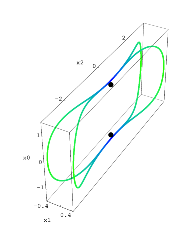
Figure 6: Plot of the two magnetic monopole loops for the gauge potential (4.22) projected onto the $x_{1}-x_{2}-x_{0}$-space (dropping the $x_{3}$-component). Rotations with angle $\pi$ around the $x_{1}$- , $x_{2}$- and $x_{3}$-axis interchange the different monopole branches. The thick dots show the positions of the instantons.

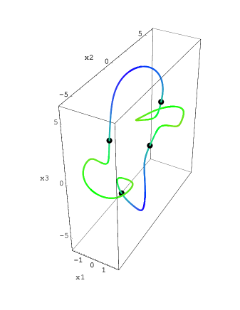
Figure 7: Plot of the vortex in the time-slice $x_{0}=0$. The thick dots on the vortex show the positions of the magnetic monopoles.

At the end we changed the gauge potential (4.22) by a factor $2$. The result is a higher field strength. Accordingly, after Laplacian Abelian gauge fixing, the number of magnetic monopole loops increases. We identified $6$ magnetic monopole loops — two of them are larger and intersect each other on the $x_{0}$ axis (similar as in the case with gauge potential $A_{{\mathrm{I}A}}$, cf. (4.22)), while the other four monopole loops are smaller and separated from each other, cf. figures 9,9. The set of all magnetic monopole loops is again symmetric with respect to rotations with angle $\pi$ around the $x_{1}$-, $x_{2}$- and $x_{3}$-axis.

Figure 8: Plot of the $r-x_{0}$-projection ($r=\sqrt{x_{1}^{2}+x_{2}^{2}+x_{3}^{2}}$) of one of the $4$ small magnetic monopole loops and one half of one of the $2$ large magnetic monopole loops for the gauge potential $2A_{{\mathrm{IA}}}$. The crosses show the positions of the instanton centers.

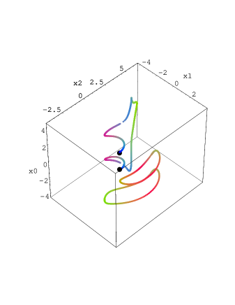
Figure 9: $3$-dimensional plot of the monopole loops for the doubled instanton-anti-instanton gauge potential projected onto the $x_{1}-x_{2}-x_{0}$ space. Only one of the $4$ small magnetic monopole loops and one half of the $2$ large magnetic monopole loops are plotted. The remaining part of the monopole loop is obtained by rotations with angle $\pi$ around the $x_{1}$-, $x_{2}$- and $x_{3}$-axes, respectively. The thick dots show the positions of the instanton centers.

5 Concluding remarks

We have studied various field configurations relevant for the infrared sector of QCD in the continuum analog of Laplacian (Abelian and) center gauges. While the gauge does not detect center vortices for single instantons it identifies center vortices for merons and composite instanton-anti-instanton configurations. The absence of center vortices in single instantons is somewhat expected if center vortices are responsible for confinement, which is, however, not explained by instantons. Furthermore we have also shown that for highly symmetric field configurations Laplacian center gauge does not necessarily provide a very faithful method for detecting their vortex content, because these configurations lie mostly on the Gribov horizon. A better detector for center vortices is the Wilson loop. From the study of the Wilson loop we have provided evidence that merons can be interpreted as self-intersection points of center vortices.

References

- [1]
- [2] G. Parisi, Phys. Rev. D11, 970 (1975).
- [3] S. Mandelstam, Phys. Rep. 23, 245 (1976).
- [4] G. ‘t Hooft, in: High Energy Physics, Proceedings of the EPS International Conference, Palermo 1975, A. Zichichi, ed., Editrice Compositori, Bologna 1976.
- [5] G. ‘t Hooft, Nucl. Phys. B138, 1 (1978).
- [6] G. Mack, and V. B. Petkova, Ann. Phys. (NY) 123, 442 (1979).
- [7] G. ‘t Hooft, Nucl. Phys. B190, 455 (1981).
- [8] T. Suzuki, and I. Yotsuyanagi, Phys. Rev. D42, 4257 (1990).
- [9] S. Hioki, S. Kitahara, S. Kiura, Y. Matsubara, O. Miyamura, S. Ohno and T. Suzuki, Phys. Lett. B272, 326 (1991).
- [10] G. S. Bali, C. Schlichter, and K. Schilling, Prog. Theor. Phys. Suppl. 131, 645 (1998) and references therein.
- [11] K. Bernstein, G. Di Cecio, and R. W. Haymaker, Phys. Rev. D55, 6730 (1997).
- [12] A. Di Giacomo, B. Lucini, L. Montesi, and G. Paffuti, Phys. Rev. D61, 034503 (2000).
- [13] L. Del Debbio, M. Faber, J. Greensite, and Š. Olejník, Phys. Rev. D55, 2298 (1997).
- [14] L. Del Debbio, M. Faber, J. Giedt, J. Greensite, and S. Olejnik, Phys. Rev. D58, 094501 (1998).
- [15] M. Engelhardt, and H. Reinhardt, Nucl. Phys. B567, 249 (2000).
- [16] Ph. de Forcrand, and M. D’Elia, Phys. Rev. Lett. 82, 4582 (1999).
- [17] K. Langfeld, O. Tennert, M. Engelhardt, and H. Reinhardt, Phys. Lett. B452, 301 (1999).
- [18] M. Engelhardt, K. Langfeld, H. Reinhardt, and O. Tennert, Phys. Rev. D61, 054504 (2000).
- [19] T. G. Kovacs, and E. T. Tomboulis, Phys. Rev. Lett. 85, 704 (2000).
- [20] V. Gribov, Nucl. Phys. B139, 1 (1978).
- [21] F. Bruckmann, T. Heinzl, T. Tok, and A. Wipf, Nucl. Phys. B584, 589 (2000).
- [22] J. C. Vink, U.-J. Wiese, Phys. Lett. B289, 122 (1992).
- [23] A. J. van der Sijs, Nucl. Phys. Proc.-Suppl. 53, 535 (1997).
- [24] C. Alexandrou, M. D’Elia, and P. de Forcrand, Nucl. Phys. Proc.-Suppl. 83, 4582 (2000).
- [25] C. Alexandrou, P. de Forcrand, and M. D’Elia, Nucl. Phys. A663, 1031 (2000)
- [26] C. G. Callan, Jr., R. F. Dashen, and D. J. Gross, Phys. Rev. D17, 2717 (1978)
- [27] C. G. Callan, Jr., R. F. Dashen, and D. J. Gross, Phys. Rev. D19, 1826 (1979)
- [28] M. N. Chernodub, and F. V. Gubarev, JETP Lett. 62, 100 (1995).
- [29] A. Hart, and M. Teper, Phys. Lett. B371, 261 (1996).
- [30] R. C. Brower, K. N. Orginos, and C.-I. Tan, Phys. Rev. D55, 6313 (1997).
- [31] V. Bornyakov, and G. Schierholz, Phys. Lett. B384, 190 (1996).
- [32] F. Bruckmann, T. Heinzl, T. Vekua, and A. Wipf, Magnetic monopoles vs. Hopf defects in the Laplacian (Abelian) gauge, hep-th/0007119.
- [33] N. Weiss, Phys. Rev. D24, 475 (1981).
- [34] H. Suganuma, K. Itakura, and H. Toki, Instantons and QCD monopole trajectory in the Abelian dominating system, hep-th/9512141.
- [35] H. Reinhardt, Nucl. Phys. B503, 505 (1997).
- [36] O. Jahn, and F. Lenz, Phys. Rev. D58, 085006 (1998).
- [37] C. Ford, U. G. Mitreuter, T. Tok, A. Wipf, and J. M. Pawlowski, Ann. Phys. (NY) 269, 26 (1998); C. Ford, T. Tok, and A. Wipf, Phys. Lett. B456, 155 (1999); Nucl. Phys. B548, 585 (1999).
- [38] M. Quandt, H. Reinhardt, and A. Schäfke, Phys. Lett. B446, 290 (1999).
- [39] Ph. de Forcrand, and M. Pepe, Center Vortices and Monopoles without lattice Gribov copies, hep-lat/0008016.
- [40] A. S. Kronfeld, G. Schierholz, and U.-J. Wiese, Nucl. Phys. B293, 461 (1987).
- [41] J. Arafune, P.G.O. Freund, and C.J. Goebel, J. Math. Phys. 16, 433 (1975).
- [42] F. Palumbo, Phys. Lett. B173, 81 (1986), Phys. Lett. B243, 109 (1990).
- [43] E. Witten, Nucl. Phys. B156, 269 (1979).
- [44] G. Veneziano, Nucl. Phys. B159, 213 (1979).
- [45] J. V. Steele, and J. W. Negele, Meron pairs and fermionic zero modes, hep-lat/0007006.
- [46] G. ‘t Hooft, Phys. Rev. D14, 3432 (1976).
- [47] D. A. Varshalovich, A. N. Moskalev, and V. K. Khersonskii, Quantum Theory of Angular Momentum (World Scientific Publishing, Singapore, 1988).