Hedgehogs in higher dimensional gravity with curvature self-interactions

Abstract

Static solutions of the higher dimensional Einstein-Hilbert gravity supplemented by quadratic curvature self-interactions are discussed in the presence of hedgehog configurations along the transverse dimensions. The quadratic part of the action is parametrized in terms of the (ghost-free) Euler-Gauss-Bonnet curvature invariant. Spherically symmetric profiles of the transverse metric admit exponentially decaying warp factors both for positive and negative bulk cosmological constants.

Preprint Number: UNIL-IPT-00-20, September 2000

I Formulation of the problem

The idea that gravitational and gauge interactions can be unified in more than four space-time dimensions has been widely explored in various frameworks [1]. More recently, internal dimensions have been analyzed in connection with possible alternatives of Kaluza-Klein compactification [2, 3] ( see also [4, 5] and [6]).

In this context [3, 5] our $(3+1)$-dimensional world might be interpreted as the internal space-time associated with a topological defect living in a higher dimensional manifold. This possibility has been scrutinized from different perspectives. New solutions of the Einstein field equations (originally studied in the case of two transverse dimensions [3]) were obtained in the case when the number of transverse dimensions $n$ is equal to two [7, 8, 9] or even larger than two [10, 11] (see also [12] for an earlier work on $n>2$ transverse dimensions).

The description of gravity assumed in the discussion of [10, 11] relies on the Einstein-Hilbert action supplemented by a bulk cosmological constant and by matter sources (describing static topological defects living in the internal space). The aim of this paper is to discuss the scenario analyzed in [10, 11] in the framework of a different gravity theory where quadratic self-interactions are consistently included in the higher dimensional action. The form of the gravity action considered in the present paper will then be

$$S_{\rm g}=\int d^{D}x\,\sqrt{-g}\,\biggl{[}-\frac{M^{D-2}}{2}\,R+\Lambda_{D}-\alpha^{\prime}R_{\rm EGB}^{2}\biggr{]},$$ (1.1)

where $R$ is the curvature scalar in $D$-dimensions, $\Lambda_{D}$ is the bulk cosmological constant and $R_{\rm GB}^{2}$ is the quadratic part of the action which we choose to be in the form of the Euler-Gauss-Bonnet (EGB) combination:

$$R_{\rm EGB}^{2}=R^{\beta\mu\alpha\nu}R_{\beta\mu\alpha\nu}-4\,R^{\mu\nu}R_{\mu\nu}+R^{2}.$$ (1.2)

The coupling constant appearing in front of the EGB invariant has dimensions $\alpha^{\prime}=[M^{D-4}]$. In the present analysis the full $D$-dimensional space-time will have a $(3+1)$-dimensional part and a transverse part formed by $n$ dimensions so that, dimensionally, $\alpha^{\prime}=[M]^{n}$. Convincing motivations coming from different theoretical ideas conspire towards the EGB combination [13, 14] as a possible parameterization of quadratic self-interactions in higher dimensions. In four dimensions the EGB combination is a topological term: its contribution to the action can be rearranged in a perfect four divergence which does not contribute to the classical equations of motion. In four dimensions the EGB combination coincides with the Euler invariant. In dimensions higher than four the EGB combination is not a total divergence and it does contribute to the classical equations of motion with terms containing (at most) a second derivative of the metric. Needless to say that, from a cosmological point of view, the absence of derivatives higher than the second makes tractable (without the addition of extra initial conditions) the problem of the dynamical evolution [15, 16]. In a different perspective the EGB combination leads to ghost-free nontrivial gravitational self-interactions for $D>4$ [13, 14]. Quadratic terms in the gravitational action can naturally appear for diverse reasons. In string theory the (tree-level) low energy effective action is normally supplemented by two kinds of expansions: the expansion in the dilaton coupling (leading to higher genus correction) and the expansion in the string tension $\alpha^{\prime}$ which involves the appearance of quadratic terms in the action [17] . In supergravity the EGB is required for the supersimmetrization of the Lorentz-Chern-Simons term. Higher dimensional theories with gravitational self-interactions were also investigated in the context of spontaneous compactification [21] induced by quadratic curvature corrections [22].

Consider now a $4+n$-dimensional metric consistent with four-dimensional Poincaré invariance (of the type proposed in [3]) whose line element can be written as:

$$ds^{2}=g_{\mu\nu}dx^{\mu}dx^{\nu}=\sigma(y^{a})\eta_{AB}dx^{A}dx^{B}+\gamma_{ab}dy^{a}dy^{b},$$ (1.3)

where $\sigma(y^{a})$ is a conformal factor which only depends upon the the internal coordinates $y^{a}$; $\gamma_{ab}(y)$ parameterizes the metric of the internal space and $\eta_{AB}$ is the four-dimensional Minkowski metric .

In [7] solutions of the Einstein field equations have been obtained with a bulk (negative) cosmological constant and for local (string-like) defect along the (two-dimensional) transverse space. In [10, 11] higher dimensional transverse spaces have been studied with particular attention to global (hedgehog) defects present in the transverse space.

The aim of the present paper is twofold. On one hand possible solutions of the Einstein-Hilbert theory (supplemented by quadratic self-interactions) will be studied in the case of a higher dimensional transverse space. On the other hand useful generalizations of previous results will be provided. The present analysis is, therefore, complementary to the ones of Ref. [10, 11]. Gravitational self-interactions have been studied in the case of one or two transverse dimension [19, 20], but not in the case of higher dimensional (global) defects like the ones discussed in the present paper.

The plan of the present paper is then the following. In Section II the basic equations will be derived. In Section III solutions with exponentially decreasing warp factors and spherically symmetric transverse metric will be presented. Section IV deals with some possible extensions of the results with particular attention to the case of a bulk electromagnetic field. Finally section V contains the concluding remarks.

II Basic equations

The total action of the problem at hand is given by the sum of the gravity action of Eq. (1.1) supplemented by the appropriate matter sources:

$$S=S_{\rm g}+S_{\rm m}.$$ (2.1)

By functionally deriving the action with respect to the metric we obtain the corresponding equations of motion:

$$R_{\mu\nu}-\frac{1}{2}g_{\mu\nu}R=-\frac{\Lambda}{M^{n+2}}g_{\mu\nu}+\frac{T_{\mu\nu}}{M^{n+2}}+\frac{2\alpha^{\prime}}{M^{n+2}}{\cal Q}_{\mu\nu},$$ (2.2)

$$\nabla_{\mu}T^{\mu\nu}=0,$$ (2.3)

where $T_{\mu\nu}$ contains the contribution of the matter sources (obeying covariant conservation laws) and where ${\cal Q}_{\mu\nu}$ contains the contribution of the EGB which turns out to be [14]

$${\cal Q}_{\mu\nu}=\frac{1}{2}g_{\mu\nu}R_{\rm EGB}^{2}-2R~{}R_{\mu\nu}+4R_{\mu\alpha}~{}R^{\alpha}_{~{}~{}\nu}+4R_{\alpha\beta}~{}R^{\alpha\,\,\,\beta}_{\,\,\,\mu\,\,\,\nu}-2R_{\mu\alpha\beta\gamma}~{}R_{\nu}^{~{}~{}\alpha\beta\gamma}.$$ (2.4)

In Eq. (2.4) it has been assumed that the physical cosmological constant vanishes. In other words, the condition

$$R^{(4)}_{AB}-\frac{1}{2}g_{AB}R^{(4)}=0,$$ (2.5)

will be implemented. A hedgehog living along three transverse dimensions will be described through a triplet of scalars $(\phi^{1},\,\,\phi^{2},\,\,\phi^{3})$ whose potential can be chosen to be:

$$V(\phi)=\frac{\lambda}{4}(\phi^{a}\phi^{a}-v^{2}),$$ (2.6)

where, as previously mentioned, the (small) Latin indices run over the transverse directions. Outside the core the hedgehog ansatz

$$\phi^{a}(\rho)=v\,\,\frac{\rho^{a}}{\rho}$$ (2.7)

will be considered ($\rho^{a}/\rho$ is the unit vector along the transverse space). The three-dimensional metric of the transverse space will be chosen to be spherically symmetric so that the full (seven-dimensional) line element can be written as

$$ds^{2}=\sigma(\rho)\eta_{AB}dx^{A}dx^{B}+d\rho^{2}+\gamma(\rho)[d\vartheta^{2}+\sin^{2}{\vartheta}d\varphi^{2}],$$ (2.8)

with $\eta_{AB}$ being the ordinary $(3+1)$-dimensional flat space metric $[-1,~{}+,~{},+,~{}+]$ with signature “mostly plus”. Notice that $\rho\geq 0$. Consequently, the components of the energy-momentum tensor will be:

$$T_{\rho}^{\rho}=-\frac{v^{2}}{\gamma},\,\,\,\,\,\,T_{A}^{B}=-\frac{v^{2}}{\gamma}\delta_{A}^{B},$$ (2.9)

$$T_{\vartheta}^{\vartheta}=T_{\varphi}^{\varphi}=0.$$ (2.10)

The purpose of the following Section will be to study some particular solution of the system of equations (2.3) with specific attention to the role played by the quadratic corrections of Eq. (2.4).

III Solutions with exponential warp factors

Defining ${\cal H}=[\ln{\sigma}]^{\prime}$, ${\cal F}=[\ln{\gamma}]^{\prime}$, the EGB invariant can be written as

$$R_{EGB}^{2} = \biggl{[}-4{\cal F}^{3}{\cal H}-\frac{4}{\gamma}({\cal H}^{2}+4\frac{\sigma^{\prime\prime}}{\sigma})+{\cal F}^{2}{\cal H}^{2}-\frac{9}{2}{\cal H}^{4}+8{\cal F}{\cal H}\frac{\gamma^{\prime\prime}}{\gamma}$$ (3.1)

$$+ 4{\cal F}^{2}\frac{\sigma^{\prime\prime}}{\sigma}+24{\cal F}{\cal H}\frac{\sigma^{\prime\prime}}{\sigma}+12{\cal H}^{2}\biggl{(}\frac{\sigma^{\prime\prime}}{\sigma}+\frac{\gamma^{\prime\prime}}{\gamma}\biggr{)}\biggr{]}.$$ (3.2)

Consequently, using the line element (2.8), Eqs. (2.3)–(2.4) become, in components,

$${\cal F}^{\prime}+\frac{3}{2}{\cal H}^{\prime}+\frac{3}{2}{\cal H}{\cal F}+\frac{3}{2}{\cal H}^{2}+\frac{3}{4}{\cal F}^{2}-\frac{1}{\gamma}=-\biggl{(}\frac{\Lambda}{M_{7}^{5}}+\frac{v^{2}}{\gamma~{}~{}M_{7}^{5}}\biggr{)}+\frac{2\alpha^{\prime}}{M_{7}^{5}}{\cal G}_{0}(\rho),$$ (3.3)

$$\frac{{\cal F}^{2}}{4}+\frac{3}{2}{\cal H}^{2}+2{\cal H}{\cal F}-\frac{1}{\gamma}=-\biggl{(}\frac{\Lambda}{M_{7}^{5}}+\frac{v^{2}}{\gamma~{}~{}M_{7}^{5}}\biggr{)}+\frac{2\alpha^{\prime}}{M_{7}^{5}}{\cal G}_{\rho}(\rho),$$ (3.4)

$$2{\cal H}^{\prime}+\frac{{\cal F}^{\prime}}{2}+\frac{5}{2}{\cal H}^{2}+\frac{1}{4}{\cal F}^{2}+{\cal H}{\cal F}=-\frac{\Lambda}{M_{7}^{5}}+\frac{2\alpha^{\prime}}{M_{7}^{5}}{\cal G}_{\vartheta}(\rho),$$ (3.5)

$$2{\cal H}^{\prime}+\frac{{\cal F}^{\prime}}{2}+\frac{5}{2}{\cal H}^{2}+\frac{1}{4}{\cal F}^{2}+{\cal H}{\cal F}=-\frac{\Lambda}{M_{7}^{5}}+\frac{2\alpha^{\prime}}{M_{7}^{5}}{\cal G}_{\varphi}(\rho),$$ (3.6)

where

$${\cal G}_{0}(\rho) = \biggl{[}\frac{3}{2}{\cal H}{\cal F}^{3}+\frac{9}{2}{\cal H}^{3}{\cal F}+\frac{3}{4}{\cal H}^{4}+3{\cal H}{\cal F}{\cal F}^{\prime}+\frac{9}{2}{\cal H}^{2}{\cal F}^{2}$$ (3.7)

$$+ \frac{3}{2}{\cal F}^{2}{\cal H}^{\prime}+6{\cal H}{\cal F}{\cal H}^{\prime}+\frac{3}{2}{\cal H}^{2}{\cal H}^{\prime}-\frac{6}{\gamma}({\cal H}^{2}+{\cal H}^{\prime})\biggr{]},$$ (3.8)

$${\cal G}_{\rho}(\rho) = \biggl{(}\frac{3}{4}{\cal H}^{4}+6{\cal F}{\cal H}^{3}+\frac{9}{2}{\cal F}^{2}{\cal H}^{2}-\frac{6}{\gamma}{\cal H}^{2}\biggr{)},$$ (3.9)

$${\cal G}_{\vartheta}(\rho) \equiv {\cal G}_{\varphi}(\rho)=\biggl{(}\frac{3}{2}{\cal H}^{2}{\cal F}^{2}+3{\cal H}^{2}{\cal F}^{\prime}+6{\cal H}{\cal F}{\cal H}^{\prime}+6{\cal H}^{3}{\cal F}+\frac{15}{4}{\cal H}^{4}+6{\cal H}^{2}{\cal H}^{\prime}\biggr{)}.$$ (3.10)

Eqs. (3.3)–(3.6) are, respectively, the $(00)$, $(\rho~{}\rho)$, $(\vartheta~{}\vartheta)$ and $(\varphi~{}\varphi)$ components of Eq. (2.3). Notice that the ($\vartheta$,$\vartheta$) and ($\varphi$,$\varphi$) components of Eq. (2.3) lead to the same equation.

If $\alpha^{\prime}=0$ (i.e. in the absence of quadratic corrections) a particular solution of the previous system is [11]

$$\sigma{\rho}=e^{-\frac{\rho}{L}},\,\,\,\gamma(\rho)=\gamma_{L}={\rm constant}.$$ (3.11)

Inserting ${\cal H}=-1/L$ and ${\cal F}=0$, into Eqs. (3.3)–(3.6) the relations

$$L=\sqrt{-\frac{5M_{7}^{5}}{2\Lambda}},$$ (3.12)

$$\gamma_{L}=L^{2}\biggl{(}\frac{v^{2}}{M_{7}^{5}}-1\biggr{)},$$ (3.13)

can be obtained. In eq. (3.12) $\Lambda<0$ and $v^{2}/M_{7}^{5}$ is a dimensionless quantity. By now tuning $v^{2}=M_{7}^{5}$ a different solution can be obtained, namely

$${\cal F}={\cal H}=-\frac{1}{L},\,\,\,\sigma(\rho)=q~{}\gamma(\rho),$$ (3.14)

with

$$L=\sqrt{-\frac{15}{4}\frac{M_{7}^{5}}{\Lambda}},$$ (3.15)

also in this case the cosmological constant needs to be negative.

If $\alpha^{\prime}\neq 0$ new solutions can be obtained. In particular, assuming that ${\cal H}=-1/L$ and that ${\gamma}_{L}={\rm constant}$, consistency with Eqs. (3.3)–(3.6) requires

$$\frac{3}{2~{}~{}L^{2}}-\frac{1}{\gamma_{L}}=-\frac{\Lambda}{M^{5}_{7}}-\frac{v^{2}}{\gamma_{L}~{}~{}M_{7}^{5}}+\frac{2\alpha^{\prime}}{M_{7}^{5}}\,\,\biggl{(}\frac{3}{4~{}~{}L^{4}}-\frac{6}{L^{2}\,\gamma_{L}}\biggr{)},$$ (3.16)

$$2\,\frac{\Lambda}{M^{5}_{7}}\,L^{4}\,\,+\,\,5\,L^{2}\,\,-\,\,15\,\frac{\alpha^{\prime}}{M_{7}^{5}}=0,$$ (3.17)

whose solution is

$$\gamma_{L}(L)=\frac{L^{4}(M_{7}^{5}-v^{2})-12\,\alpha^{\prime}\,L^{2}}{L^{4}\Lambda+\frac{3}{2}(L^{2}M_{7}^{5}-\alpha^{\prime})},$$ (3.18)

$$L^{2}=-\frac{5}{4}\frac{M_{7}^{5}}{\Lambda}\biggl{[}1\mp\sqrt{1+\frac{24}{5}\frac{\Lambda~{}\alpha^{\prime}}{M_{7}^{10}}}\biggr{]}.$$ (3.19)

In the limit $\alpha^{\prime}\rightarrow 0$, the expression for $\gamma_{L}$ obtained in Eq. (3.13). is formally recovered. Define, for sake of simplicity, $\Lambda=\Lambda_{+}$ (if $\Lambda>0$) and $\Lambda=-\Lambda_{-}$ (if $\Lambda<0$). Then, from Eq. (3.19),

$$L_{+}=\biggl{\{}-\frac{5}{4}\frac{M_{7}^{5}}{\Lambda_{+}}\biggl{[}1-\sqrt{1+\frac{24}{5}\frac{\Lambda_{+}~{}\alpha^{\prime}}{M_{7}^{10}}}\biggr{]}\biggr{\}}^{1/2},$$ (3.20)

$$L_{-}=\biggl{\{}\frac{5}{4}\frac{M_{7}^{5}}{\Lambda_{-}}\biggl{[}1+\sqrt{1-\frac{24}{5}\frac{\Lambda_{-}~{}\alpha^{\prime}}{M_{7}^{10}}}\biggr{]}\biggr{\}}^{1/2}.$$ (3.21)

From Eq. (3.19), an exponentially decreasing warp factor can be obtained either from $L_{+}$ ( with $\Lambda>0$) or from $L_{-}$ (with $\Lambda<0$). For positive bulk cosmological constant $L_{+}$ is always defined. In the case of negative cosmological constant $L_{-}$ is defined only if

$$\frac{\alpha^{\prime}\Lambda_{-}}{M_{7}^{10}}<\frac{5}{24}.$$ (3.22)

Thus, exponentially decreasing warp factors are possible for any positive cosmological constant and for negative cosmological constants whose absolute value satisfies Eq. (3.22).

In the limit $\alpha^{\prime}\rightarrow 0$ we get $L_{-}\rightarrow 0$ and $\gamma_{L}(L_{-})\rightarrow 0$. On the contrary, for $\alpha^{\prime}\rightarrow 0$, $L_{+}\rightarrow\sqrt{-5M_{7}^{5}/2\Lambda}$ and the solution in the absence of EGB invariant is reproduced since $\gamma_{L}(L_{+})$ exactly equals the relation derived in Eq. (3.13). Therefore, the inclusion of quadratic self-interactions has a twofold effect. On one hand it generalizes the tree-level solution. On the other hand it introduces a new solution whose limit (for $\alpha^{\prime}\rightarrow 0$ ) is the (seven-dimensional) Minkowskian space.

Given a specific $L_{\pm}$, $\gamma_{L}(L_{\pm})$ can be determined through Eq. (3.18). Since the signature of the metric should be preserved $\gamma_{L}(L_{\pm})$ is required to be positive definite. Thus Eq. (3.18) together with Eqs. (3.20)–(3.21) imposes a physical bound for the scalar vacuum expectation value $v^{2}$. Using the equation satisfied by $L_{\pm}$ in the denominator of the relation (3.18) we can see that $\gamma_{L}(L_{\pm})>0$ if

$$v^{2}>\frac{L_{\pm}^{2}M_{7}^{5}-12\alpha^{\prime}}{L_{\pm}^{2}}.$$ (3.23)

A different solution to Eqs. (3.3)–(3.6) can be obtained by tuning $v^{2}=(L^{2}M_{7}^{5}-12\alpha^{\prime})/L^{2}$. In this case the $1/\gamma$ factors disappear from the equations of motion whose integration can be performed by assuming that $\sigma\propto\gamma$ or, in terms of their logarithmic derivatives, that ${\cal H}={\cal F}$. In this case the equations of motion (3.3)–(3.6) can be consistently solved assuming an exponentially decreasing warp factor. Following the same steps outlined in the previous case $L$ can be found, and it turns out to be

$$L^{2}=-\frac{15M^{5}}{8\Lambda}(1\mp\sqrt{1+\frac{32\alpha^{\prime}\Lambda}{5~{}M_{7}^{10}}}).$$ (3.24)

As in the previous the limit $\alpha^{\prime}\rightarrow 0$ can be discussed. One limit gives back the tree-level solution the other limit gives the (seven-dimensional ) Minkowski space. Notice that, again, when $\alpha^{\prime}\neq 0$ the exponential decrease in the warp factor can be achieved both with positive and negative bulk cosmological constant.

This last solution has a curvature singularity for $\rho\rightarrow\infty$. This aspect can be illustrated by computing the EGB invariant on the obtained solutions:

$$R_{EGB}^{2}=\frac{105}{2\,L^{4}}-\frac{20\,e^{\frac{\rho}{L}}}{q\,L^{2}}$$ (3.25)

where $q$ is the proportionality factor between $\sigma$ and $\gamma$ as it appears in Eq. (3.14). In spite of the singular character of the geometry the action is finite. This solution has already a singularity of the same type already without curvature self-interactions and the addition of the EGB contribution to the action does not modify this aspect.

IV Possible Extensions: electromagnetic fields

In the present section the self-interacting gravitational field will be studied in the presence of a bulk electromagnetic field. The matter action will take then the form

$$S_{\rm m}=-\frac{1}{4}\int d^{7}x\sqrt{-g}F_{\mu\nu}F^{\mu\nu}.$$ (4.1)

The equations of motion and the Bianchi identities can be written as

$$\partial_{\mu}\biggl{(}\sqrt{-g}F^{\mu\nu}\biggr{)}=0,$$ (4.2)

$$\partial_{\mu}\biggl{(}\sqrt{-g}\tilde{F}^{\mu\nu}\biggr{)}=0.$$ (4.3)

A specific magnetic field configuration will then be chosen, namely the electromagnetic field will be completely polarized along the transverse dimensions and its only non-vanishing component will be

$$F_{\vartheta\varphi}=Q\sin{\vartheta}.$$ (4.4)

where $Q$ is a constant and, as usual, ($\vartheta$,$\varphi$) label the radial coordinates of the transverse metric. Taking now into account that the relevant components of the energy-momentum tensor are

$$T_{A}^{B}=-\frac{1}{2}\frac{Q^{2}}{\gamma^{2}}\delta_{A}^{B},\,\,\,\,T_{\rho}^{\rho}=-\frac{1}{2}\frac{Q^{2}}{\gamma^{2}},\,\,\,\,T_{\vartheta}^{\vartheta}=T_{\varphi}^{\varphi}=\frac{1}{2}\frac{Q^{2}}{\gamma^{2}},$$ (4.5)

we can write the equations of motion

$${\cal F}^{\prime}+\frac{3}{2}{\cal H}^{\prime}+\frac{3}{2}{\cal H}{\cal F}+\frac{3}{2}{\cal H}^{2}+\frac{3}{4}{\cal F}^{2}-\frac{1}{\gamma}=-\biggl{(}\frac{\Lambda}{M_{7}^{5}}+\frac{Q^{2}}{2~{}\gamma^{2}~{}~{}M_{7}^{5}}\biggr{)}+\frac{2\alpha^{\prime}}{M_{7}^{5}}{\cal G}_{0}(\rho),$$ (4.6)

$$\frac{{\cal F}^{2}}{4}+\frac{3}{2}{\cal H}^{2}+2{\cal H}{\cal F}-\frac{1}{\gamma}=-\biggl{(}\frac{\Lambda}{M_{7}^{5}}+\frac{Q^{2}}{2~{}\gamma^{2}~{}~{}M_{7}^{5}}\biggr{)}+\frac{2\alpha^{\prime}}{M_{7}^{5}}{\cal G}_{\rho}(\rho),$$ (4.7)

$$2{\cal H}^{\prime}+\frac{{\cal F}^{\prime}}{2}+\frac{5}{2}{\cal H}^{2}+\frac{1}{4}{\cal F}^{2}+{\cal H}{\cal F}=-\frac{\Lambda}{M_{7}^{5}}+\frac{Q^{2}}{2~{}\gamma^{2}~{}~{}M_{7}^{5}}+\frac{2\alpha^{\prime}}{M_{7}^{5}}{\cal G}_{\vartheta}(\rho),$$ (4.8)

[the ${\cal G}$ functions being the same as the ones of Eqs. (3.8)–(3.10)].

A solution of the form

$${\cal H}=-\frac{1}{L},\,\,\,\gamma=\gamma_{L},$$ (4.9)

will then be analyzed ($L$ and $\gamma_{L}$ are, as in the previous Section, two positive constants). In the absence of curvature corrections this solution has been discussed in [11].

From Eqs. (4.6)–(4.8) the following relations can then be obtained

$$9~{}d~{}x^{4}+2y(1-6~{}d~{}x^{2})-8~{}x^{2}-4~{}a=0,$$ (4.10)

$$3~{}d~{}x^{4}-y~{}(1-6~{}d~{}x^{2})-x^{2}+b~{}y^{2}=0,$$ (4.11)

where, for simplicity, we define

$$x=1/L,\,\,\,y=1/\gamma_{L},\,\,\,\ a=\frac{\Lambda}{M_{7}^{5}},\,\,\,b=\frac{Q^{2}}{M_{7}^{5}},\,\,\,\,d=\frac{2\alpha^{\prime}}{M_{7}^{5}}.$$ (4.12)

Eqs.(4.10)–(4.11) are difficult to solve, in general. They can be numerically solved for specific values of the parameters. Also in this case both positive and negative cosmological constants lead to exponentially decreasing warp factors.

We can illustrate this point in the following way. Working in (natural) gravitational units (i.e. $M_{7}=1$) solutions of the two algebraic equations (4.10) and (4.11) can be analyzed for the cases where the roots are simultaneously positive. Different specific values of $b$ and $d$ can be chosen. Keeping $d$ and $b$ fixed, the value of $a$ can be changed from positive to negative. Both for positive and negative $a$ (corresponding to positive and negative cosmological constants), pairs of positive roots of Eqs. (4.10)–(4.11) can be found. For instance, choosing $b=0.1$ and $d=0.1$, one gets two positive pairs of roots both for positive and negative $a$

$$(y,x)\equiv(5.006,~{}~{}1.036),\,\,\,\,{\rm for}\,\,a=-1,\,\,(y,x)\equiv(6.961,~{}~{}0.792),\,\,\,\,{\rm for}\,\,a=1,\,\,$$ (4.13)

Different sets of parameters can be chosen with similar conclusions.

FIG. 1.: The system of Eqs. (4.10)–(4.11) is illustrated for $b=d=0.1$ (in units $M_{7}=1$ ) for different values of $a$.

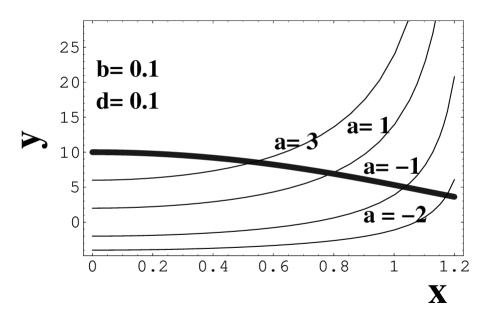
The value of $a$ can be changed (for fixed $d$ and $b$) and, in this way, the space of the possible solutions can be explored. In Fig. 1 this point is illustrated. With the thin lines the relation between $y$ and $x$ is plotted (for different values of $a$) according to Eq. (4.10). With the thick line the relation between $y$ and $x$ following from Eq. (4.11) is reported. In Fig. 1 $b=0.1$ and $d=0.1$ are fixed. The intersections of the thin lines with the thick line will give the (real) roots of the system for different values of $a$. We can observe that the intersections, in the example of Fig. 1, all lead to positive roots. Notice that Eq. (4.11) does not contain $a$ (i.e. the cosmological constant) but only $b$ and $c$ (i.e. $Q$ and $\alpha^{\prime}$). This argument shows that positive and negative cosmological constants lead to consistent solutions. In order to fully explore the space of the solution the values of $b$ and $d$ should change.

V Concluding remarks

In this paper solutions of the Einstein field equations with EGB self-interactions have been studied when a hedgehog configuration is present in the (transverse) higher dimensional space. The occurrence of exponentially decreasing warp factors has been pointed out. If quadratic self-interactions are absent, exponentially decreasing warp factors arise only for negative bulk cosmological constant. If quadratic self-interactions are present such a behavior is allowed both for positive and negative cosmological constants.

Two specific classes of solution have been examined. In the first class of solutions the functions describing the variation of the metric along the transverse coordinates are constant. In the second class of solutions the metric functions of the transverse space change with the distance from the core of the hedgehog. In this case the space-time is singular at large distances even in the presence of the EGB self-interactions.

We also discussed similar solutions in the case of a specific magnetic field configuration completely polarized along the transverse dimensions. Also in this case exponentially decreasing warp factors are stable towards quadratic self-interactions and can arise for positive and negative cosmological constants.

Ackwoledgments

The author would like to thank M. E. Shaposhnikov for interesting discussions.

REFERENCES

- [1] . Appelquist, A. Chodos, and P. G. O. Freund, Modern Kaluza-Klein Theories (Addison-Wesley, Redwood City, CA, 1987).
- [2] V. Rubakov and M. Shaposhnikov, Phys. Lett. B 125, 136 (1983).
- [3] V. Rubakov and M. Shaposhnikov, Phys. Lett. B 125, 139 (1983).
- [4] K. Akama, in Proceedings of the Symposium on Gauge Theory and Gravitation, Nara, Japan, eds. K. Kikkawa, N. Nakanishi and H. Nariai (Springer-Verlag, 1983),[hep-th/0001113].
- [5] M. Visser, Phys. Lett. B159 (1985) 22 [hep-th/9910093].
- [6] N. Arkani-Hamed, S. Dimopoulos, G. Dvali, Phys.Lett.B 429 263 (1998); I. Antoniadis, N. Arkani-Hamed, S. Dimopoulos, G. Dvali, Phys.Lett.B 436 257 (1998); N. Arkani-Hamed, S. Dimopoulos, J. March-Russel, hep-th/9809124.
- [7] T. Gherghetta and M. Shaposhnikov, Phys.Rev.Lett. 85, 240 (2000).
- [8] A. G. Cohen and D. B. Kaplan, Phys. Lett. B 470, 52 (1999).
- [9] A. Chodos and E. Poppitz, Phys. Lett. B 471, 119 (1999).
- [10] I. Olasagasti and A. Vilenkin, Phys. Rev. D 62, 044014 (2000).
- [11] T. Gherghetta, E. Roessl, and M. E. Shaposhnikov, UNIL-IPT-0014, [hep-th/0006251].
- [12] S. Randjbar-Daemi and C. Wetterich, Phys. Lett. B 166, 65 (1986).
- [13] B. Zwiebach, Phys. Lett. B 156, 315 (1985).
- [14] D. G. Boulware and S. Deser, Phys. Rev. Lett. 55, 2656 (1985); Phys. Lett. B 175, 409 (1986).
- [15] M. Gasperini and M. Giovannini, Phys. Lett. B 287, 56 (1991).
- [16] S. Kalara and K. A. Olive, Phys. Lett B 218, 148 (1989).
- [17] M. B. Green, J. H. Schwartz, and E. Witten, Superstring Theory (Cambridge University Press, Cambridge, England, 1987).
- [18] L. Randall and R. Sundrum, Phys.Rev. Lett. 83, 3370 (1999).
- [19] N. Mavromatos and J. Rizos, [hep-th/0008074].
- [20] J. E. Kim, B Kyae and H. M. Lee, [hep-th/0004005]; I. Low and A. Zee, [hep-th/0004124]; I. Neupane, [hep-th/0008191].
- [21] P. G. O. Freund and M. A Rubin, Phys. Lett. B 97, 233 (1980); E. Cremmer, B. Julia, and J. Sherk, Phys. Lett. B 76, 409 (1978); E. Cremmer and J. Sherk, Nucl. Phys. B 108, 409 (1976).
- [22] C. Wetterich, Phys. Lett. B 113, 377 (1982); Q. Shafi and C. Wetterich, Phys. Lett. B 129, 387 (1983).