Beyond Eikonal Scattering in M(atrix)-Theory

Abstract:

We study the problem of more general kinematics for the finite $N$ M(atrix)-Model than the simple straight line motion that has been used before. This is supposed to be related to momentum transferring processes in the dual super-gravity description. We find a negative result for classical, perturbative processes and discuss briefly the possibility of instianton like quantum mechanical tunneling processes.

1 Introduction

When the M(atrix)-Model for M-Theory was proposed by Banks, Fischler, Shenker and Susskind[1] and later in a version for finite $N$ by Susskind[2] it was one of the strongest quantitative tests that it was able to reproduce graviton scattering amplitudes of eleven-dimensional supergravity. In the sequel, several authors[3, 4, 5, 6, 7, 8, 9, 10, 11, 12] were able to generalize the agreement of the famous $v^{4}/r^{7}$ amplitude to higher loop orders, polarization dependent effects and more particles. Although in the meantime, some of those results have been given an interpretation in terms of supersymmetric non-renormalization theorems [13, 14] and it was shown that the agreement does not persist if one includes quantum corrections on the sugra side[15], to our understanding the ultimate fate of the M(atrix) conjecture, whether it is applicable at least in a certain regime or the agreement — especially of the finite $N$ version that is under computational control — was a mere coincidence is not settled, yet.

All the calculations mentioned above have a common kinematical restriction: They compute quantum fluctuations around a classical solution that represents free particles, implying that one has always only studied the limit of vanishing momentum transfer. In more technical terms, what has been actually computed is a phase shift in the eikonal regime. On the sugra side, this either corresponds to a source-probe approximation or, in the more general language of Feynman graphs, to T-channel scattering[11], see also the discussion in [15].

In beginning of this study, we were trying to get rid of this rather strict kinematical restriction. But it turned out, at least for finite $N$, that this is impossible, at least for the classical situation. Rather, one has to resort to quantum mechanical tunneling processes. This means, momentum transfer is always a non-perturbative process that vanishes in the classical limit.

As the M(atrix)-Model is formulated in the light-cone frame, there are two different flavors of momentum to both of which our claim applies: First, there is ordinary momentum in the transversal directions and second, there is momentum in the light like direction that appears as the the size $N$ of the matrices, or more specifically as the sizes $N_{I}$ of the blocks of block diagonal matrices representing particles with $N_{I}$ units of light-cone momentum. Both kinds of momenta are related by a $M^{-i}$ Lorentz boost that is non-trivial in light-cone coordinates. While the transfer of the latter kind has long been suspected to be a non-perturbative process there was no reason to assume the transfer of transversal momentum to be impossible classically.

To render these statement more concrete let us recall the Lagrangian of the M(atrix)-Model

$$L=\hbox{Tr}\left(\frac{1}{2}\dot{X}^{i}\dot{X}^{i}+\frac{1}{4}[X^{i},X^{j}][X_{i},X_{j}]-i\bar{\psi}\dot{\psi}+\bar{\psi}\gamma^{i}[X_{i},\psi]\right)$$ (1)

For the purpose of this investigation we can ignore the fermions. The potential energy of the bosons

$$V=-\frac{1}{4}[X^{i},X^{j}][X_{i},X_{j}]$$

is non-negative and vanishes if all the $X^{i}$ mutually commute. Thus, a solution to the equations of motion (further on termed “the trivial”) is that of diagonal matrices with linear dependence on time:

$$X_{triv}^{i}(t)=\pmatrix{r^{i}_{1}(t)&&\cr&\ddots&\cr&&r^{i}_{N}(t)\cr},\qquad r^{i}_{a}(t)=b^{i}_{a}+v^{i}_{a}t$$

The important observation of [1, 16] was to interpret these diagonal matrix entries as the time-dependent coordinates of $N$ partons (or D0-particles) in ${\mathbb{R}}^{9}$. For the trivial solution the motion of the partons is free (at least classically), $\vec{b}_{a}$ is the impact parameter of parton $a$ and $\vec{v}_{a}$ is its velocity.

The usual procedure is now to employ the background field method by splitting the quantum field $X^{i}$ into this classical part and small quantum fluctuations:

$$X^{i}(t)=X^{i}_{triv}(t)+Y^{i}(t)$$

The vacuum effective action of the $Y^{i}$ is then the effective action of $N$ partons with asymptotic states described by the $\vec{b}_{a}$ and $\vec{v}_{a}$. Performing this calculation at the one-loop level yields the famous $v^{4}/r^{7}$ potential of 11D supergravity.

It is important to include the fermions in the quantum part of this computation whereas in the classical background, they only encode polarizations of the gravitons[6, 8]. The leading order interaction is always given by a purely bosonic background. Therefore, for the purpose of our investigation which aims to generalize the classical background we do not have to take into account the fermions.

Due to the nature of the trivial solution, it was so far only possible to compute the quantum effective action for states for which the in and the out state are identical and differ only by a mere phase. In the supergravity language this means that no momentum has been transferred and the scattering has been performed in the T-channel.

In the setting of the background field method, in order to drop this strong kinematical restriction one would have to find a classical solution with the appropriate asymptotic behavior and perform the fluctuation analysis in this background.

As we are aiming at scattering processes we are not interested in bound solutions that to not approach infinity for asymptotic times. Now we can formulate the problem investigated in this paper in a gauge independent way: We are looking for solutions of the bosonic equations of motion

$$\ddot{X}^{i}=-[X^{j},[X^{i},X^{j}]]$$

that escape to infinity, i.e.

$$R^{2}(t):=\hbox{Tr}\left(X^{i}(t)X^{i}(t)\right),\qquad\lim_{t\to\pm\infty}R^{2}(t)=\infty.$$

Due to the nature of the potential, impact parameters and velocities will again be well defined for asymptotic times.

As it will turn out, only the trivial solution which is characterized by the exact vanishing of the potential energy for all times fulfills these requirements. Thus, it is impossible to transfer momentum of any kind in the finite $N$ matrix model, at least in perturbative processes. This is surprising as one might well have imagined many more, possibly very complicated, classical solutions that asymptotically escape along the valleys of the potential.

It is important to point out that this result only applies to the finite $N$ version of the M(atrix)-Model. For infinite $N$, one can T-dualize one direction and obtain M(atrix)-String-Theory of [17]. There, the existence of non-trivial scattering solutions is well known[18, 19, 20].

In the following section, we will present our argument for a highly simplified model. This will be done in some detail, as in section three, the discussion of the full model can be reduced to this simplified case. In section four, we will mention some results for the Wick rotated model, there we will find instanton like processes that are classically forbidden. In a final section, we collect our conclusions.

2 The Toy Model

In [21] a simple toy model that mimics the quartic interactions found in the M(atrix)-Model was introduced. Here in this section, we will develop the main strategy we are going to follow. This is done in quite some detail not only for pedagogical reasons but later it will turn out that the more general case can in fact be reduced to the discussion of the toy model.

In the toy model, there are only two real degrees of freedom denoted by $x$ and $y$ with a Hamilton function

$$H=\frac{1}{2}\left(\dot{x}^{2}+\dot{y}^{2}+x^{2}y^{2}\right)$$

Although this is symmetric in $x$ and $y$ one should think of $x$ representing a coordinate along the valley while $y$ represents a coordinate transversal to the valley.

This toy model can be understood as a truncation of the M(atrix)-Model as follows: Let $e_{1},e_{2}\in u(N)$ be two constant matrices that obey

$$\hbox{Tr}(e_{A},e_{B})=\delta_{AB},\qquad[e_{1},e_{2}]\neq 0.$$

Then, with the ansatz

$$X^{1}(t)=x(t)e_{1},\qquad X^{2}(t)=y(t)e_{2},\qquad X^{i}=0\hbox{ for }i>1$$

we recover the toy model. By numerical investigations in the context of QCD it has been known for a long time that this model generically exhibits chaotic behavior. Thus, we cannot hope to find exact solutions except in very singular initial conditions. Nevertheless, we will be able to make statement about properties of the general solution.

Just as in the full model, the potential

$$V=\frac{1}{2}x^{2}y^{2}$$

has valleys that reach infinity and become narrower away from the “stadium”. More precisely, transversal to the valley, the potential is quadratic with curvature proportional to the distance from the origin.

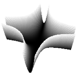
Figure 1: The potential of the toy-model

This can also be seen from the equations of motion

$$\ddot{x}=-xy^{2},\qquad\ddot{y}=-yx^{2}.$$

As in the full model, there is a trivial solution if both sides of the equations vanish identically:

$$x(t)=b+vt,\qquad y(t)=0\qquad\hbox{or }x\leftrightarrow y,$$

as the ansatz above encompasses the trivial solution of the M(atrix)-Model. As for the full model, we ask if there are further scattering solutions in the sense that

$$R(t)^{2}=x^{2}+y^{2}$$

goes to infinity for early and late times. This limit is meant in the usual sense that for each $R_{0}$ there is a $T$ such that $R(t)^{2}>R_{0}$ if $|t|>T$. We are not interested in solutions that enter the valleys but always return to the “stadium” around the origin after every such excursion, although $R(t)$ might not be bounded for such solutions.

We can use the $x\leftrightarrow\pm y$ symmetry to assume without loss of generality that the solution escapes along the positive $x$-axis for late times. From the equation of motion, we see that also $\dot{x}$ has to be positive after $T$ because otherwise the velocity will stay negative until $x=0$ and we are back to the stadium again. As we have argued above, we expect a motion that is mainly directed along the $x$-axis but with small oscillations in $y$ that are bound by the valleys. There are two possible scenarios: Either these oscillations will get smaller and smaller as the valleys are getting narrower and narrower or the oscillations are so strong that, eventually, the component of the gradient of the potential in negative $x$ direction off the bottom of the valley will stop the motion in the $x$-direction and force the particle to return to the stadium.

Numerical evolutions of the equations of motion indicate that the latter behavior is generic but we would like to investigate if there can be exceptions other than the trivial $y=0$ solution we have given above.

Figure 2: A numerical example: The solution of the toy model returns to the stadium

It is instructive to split the energy into two contributions coming from the motions in the $x$ and $y$ direction:

$$E=E_{x}+E_{y},\qquad E_{x}=\frac{1}{2}\dot{x}^{2},\qquad E_{y}=\frac{1}{2}\left(\dot{y}^{2}+x^{2}y^{2}\right)$$

Taking the time derivative,

$$\dot{E}_{y}=-\dot{E}_{x}=-\ddot{x}\dot{x}=x\dot{x}y^{2}\geq 0$$

where we used the assumptions $x>0$ and $\dot{x}>0$ from above. We see that energy is transferred constantly from the $x$ motion to the oscillations in the $y$ direction. Thus, if we took the energy $E_{y}$ to be constant we would underestimate the oscillations.

Let us recall one fact about the harmonic oscillator: It follows from the virial theorem $\langle E_{\rm kin}\rangle=\langle E_{pot}\rangle$ that the time average of the square of the oscillating variable $\langle\phi^{2}\rangle$ is given by

$$\langle\phi^{2}\rangle={E\over\omega^{2}}$$ (2)

in terms of the energy $E$ and the frequency $\omega$. Since $x$, the frequency of the oscillations in $y$, is assumed to go to infinity, $\frac{1}{x}$, the timescale of the oscillations, is going to zero. Thus, for late times, the variation of the frequency during one period of the oscillation becomes smaller and smaller. Therefore, in the equation of motion for $x$, we can replace the effect of the oscillations by the average over one period and use 2:

$$\ddot{x}=-xy^{2}\approx-x\langle y^{2}\rangle=-x{E_{y}\over x^{2}}=-{E_{y}\over x}$$

This force on $x$ can be described by an effective potential as

$$V_{\rm eff}(x)=E_{y}\log x.$$

Figure 3: The effective potential

As the logarithm grows without bound, the motion in $x$ will hit a potential barrier no matter how big the total energy $E$ is. The only exception would be that $E_{y}=0$ but this is again the trivial solution without oscillations. Therefore, we do not expect to find any other solutions that escape to infinity.

One might worry that the above reasoning using the adiabatic time averaging might be not justified. Therefore, we will give a more formal proof of the non-existence of scattering solutions, next. To this end, we will proceed along the lines of the previous heuristic argument, but without using any a priori knowledge about the solution. Therefore, we cannot employ the expressions for the harmonic oscillator in the $y$ direction.

Our strategy will be to assume that there is a solution $(x(t),y(t))$ with $E_{y}>0$ for which $x(t)$ goes to infinity as $t\to\infty$, and to show that this assumption leads to a contradiction. Namely, we will show that under these assumptions

$$\int_{0}^{\infty}dt\,\ddot{x}=-\infty.$$

This implies that any velocity in the $x$ direction will be stopped and $x$ will eventually become negative again. Thus, only the trivial solutions mentioned above will escape to infinity. Of course, as the model is invariant under time reversal, this also means that every solution that comes from $x=-\infty$ in the past has to be trivial.

To begin with, let us recall that we can assume $x$ to be arbitrarily large and that $\dot{x}$ is positive. Furthermore, $E_{y}$ is strictly increasing in time and since the total energy is conserved, all velocities and $y$ are bounded by constants determined by the initial conditions.

For some $t_{0}$, label the $y$-axis such that $y(t_{0})\leq 0$. The first thing to notice is that the retraction force is bounded by the force of the harmonic oscillator of the “momentary” frequency $\omega_{0}=x(t_{0})$ as long as $y$ is negative. But as a harmonic oscillator returns to $0$ within the next time interval of length $\pi/\omega_{0}$, the $y$ motion has to cross the $x$ axis within this interval of time , too. Let us call this moment of $y=0$ the time $t=0$.

Comparing with the harmonic oscillator once more, we can conclude that the motion again is bounded from above by that of the harmonic oscillator and that $y$ will eventually return to $0$ at some moment $0<t_{1}<\pi/\omega_{0}$.

Figure 4: Upper and lower bounds on $y(t)$

Now, we are going to estimate the retarding effect of the oscillations in $y$ on the motion in $x$. Since we are going to show that the retardation is strong enough to stop the motion in $x$ we have to give a lower bound on $y$. At $t=0$, the velocity $\dot{y}$ is positive. Any trial function $\tilde{y}$ with $\tilde{y}(0)=0$, $\dot{\tilde{y}}(0)=\dot{y}(0)$, and $\ddot{\tilde{y}}(t)<\ddot{y}(t)$ will have this property. As the kinetic energy is bounded from above, so is the velocity. Thus, by assuming $x(0)$ large enough, we know that $x(t)$ cannot double over one period. Hence, with the help of the inequality

$$-\ddot{y}(t)\leq 4t\dot{y}(0)x(0)^{2},$$

which holds because assuming the velocity in $y$ to be constant is an overestimate, we can underestimate $y(t)$ by truncating its Taylor series at the cubic order

$$y(t)\geq\sqrt{2E_{y}}t-{1\over 3}\sqrt{2E_{y}}x(0)^{2}t^{3}.$$

Here, we have used the equation of motion to see that there is no quadratic term in $t$. The right hand side is positive for $t<\sqrt{3}/x(0)$. Therefore, we have the following underestimate for the deceleration in $x$:

$$\int_{0}^{\sqrt{3}/x(0)}dt\,x(t)y(t)^{2} > x(0)\int_{0}^{\sqrt{3}/x(0)}dt\,y(t)^{2}$$

$$> 2E_{y}x(0)\int_{0}^{\sqrt{3}/x(0)}dt\,\left(t-\frac{1}{3}x(0)^{2}t^{3}\right)^{2}$$

$$= {16\sqrt{3}E_{y}\over 35x(0)^{2}}.$$

This is the deceleration for one half of a quasi-cycle of the $y$ motion. We have to sum the contributions of all the cycles. At first sight, this sum (which should be thought of as an integral over $x$!) is convergent because the contribution is proportional to $1/x^{2}$. But it is important to note that this contribution comes from the interval $[0,t_{1}]$ and its length is bounded by $\pi/x(0)$. Therefore, the average value is bounded from below by

$${16\sqrt{3}E_{y}\over 35\pi x(0)}$$

for the cycle beginning at $t=0$. To sum the contribution from all values of $x$ one has to sum a logarithmically divergent harmonic sum. This is in accordance with the logarithmic divergence we expected from the heuristic argument.

Hence we found that, however large $\dot{x}$ and however small the non-vanishing motion in $y$ is, the motion in $x$ will eventually be stopped which is the contradiction we were looking for. Therefore, we can conclude that the only motions that reach infinity are those along straight lines.

This argument has a straight forward generalization to more than two variables: First, we can increase the number of degrees of freedom that play the rôle of $y$ above:

$$H=\frac{1}{2}\left(\dot{x}^{2}+\sum_{i}\dot{y}_{i}^{2}+x^{2}\sum_{i}y_{i}^{2}\right)$$

The one dimensional harmonic oscillator is generalized to a multidimensional harmonic oscillator of which the orbits are ellipses. A simple way to see this is to introduce polar coordinates for the $y_{i}$ and observe that for the radial coordinate there is a centrifugal term that prevents the oscillator from approaching the origin. As the deceleration force on $x$ is proportional to the square of the radial coordinate, the true, time-dependent force is bounded from below from the constant force that corresponds to the minimal distance to the origin in $y_{i}$-space.

In the case of vanishing angular momentum in $y_{i}$ space, the motion is effectively one dimensional and we are back to the original toy model discussed above.

A more “democratic” generalization is to consider the Hamiltonian

$$H=\frac{1}{2}\left(\sum_{i}\dot{x}_{i}^{2}+\sum_{i\neq j}x_{i}^{2}x_{j}^{2}\right).$$

Again, by symmetry, we can assume that the solution escapes along the positive $x_{1}$ direction. Using the same argument as above we can conclude that

$$x_{1}\sim R=\sqrt{\sum_{i}x_{i}^{2}}$$

and again, as the potential energy is bounded by the total energy

$$x_{i}\sim\frac{\sqrt{E}}{R}$$

for $i>1$. The equation of motion for $x_{1}$ is the same as for $x$ in the first generalization above, whereas in

$$\ddot{x}_{i}=-x_{i}\sum_{j\neq i}x_{j}^{2}$$

the term with $j=1$ that corresponds to the equation of motion for $y_{i}$ above dominates the other terms by four orders of $R$. Thus, in the limit of late times and therefore large $R$, this second generalization reduces to the first.

3 The full model

Before starting to discuss how to extend the proof to the full model, let apply a slight reformulation: It will be enough to consider the two particle case as here one would already expect solutions that exchange transversal momenta, i.e. that have different velocities in the in compared to the out state. Furthermore, we are not interested in the center of mass motion so we can separate off the diagonal $U(1)$ and end up with a $su(2)$ model. Next, we decompose everything in terms of the Pauli matrix basis and use a vector notation for $su(2)$ indices. This turns the bosonic Lagrangian 1 into

$$L = \frac{1}{2}\dot{\vec{X}^{2}}\cdot\dot{\vec{X}^{2}}-\frac{1}{4}\|\vec{X}^{i}\times\vec{X}^{j}\|^{2}$$

$$= \frac{1}{2}\dot{\vec{X}^{2}}\cdot\dot{\vec{X}^{2}}-\frac{1}{4}\left(\sum_{i\neq j}\|\vec{X}^{i}\|^{2}\|\vec{X}^{j}\|^{2}-(\vec{X}^{i}\cdot\vec{X}^{j})^{2}\right)$$

Note that for any given instant of time, the second term in the potential can be made to vanish by a choice of coordinates in ${\mathbb{R}}^{9}$ that diagonalizes the symmetric matrix

$$M^{ij}=\vec{X}^{i}\cdot\vec{X}^{j}$$

In this choice of gauge, the model already looks similar to the second generalization of the toy model in the previous section. Unfortunately, this gauge is not obeyed by time evolution.

The toy model enjoys one important simplification compared to the full M(atrix)-Model: There is no gauge freedom, the valleys are along the $x$- and $y$-axes whereas the global $SO(9)\times SU(N)$ symmetry allows one to rotate the valleys in any possible direction. The direction of the valleys is therefore dynamically determined and one should use appropriate variables to deal with this symmetry. Furthermore, one could imagine a solution in which the matrices cannot asymptotically be brought to diagonal form because there is a non-vanishing motion in the $SU(N)$ directions that would destroy any choice of gauge at later times.

To approach these difficulties, let us first discuss another simplified model that now contains all qualitative features of the full M(atrix)-Model; this allows one to translate the argument directly to the full M(atrix)-Model, but we prefer to present the approach in this model for notational simplicity.

The degrees of freedom are two two-vectors $\vec{X}_{a}(t)\in{\mathbb{R}}^{2}$ with $a=1,2$. The Lagrangian is given by (note the close similarity to the Lagrangian of the $SU(2)$-M(atrix)-Model in the reformulation given above!)

$$L=\frac{1}{2}\left(\|\dot{\vec{X}_{1}}{}\|^{2}+\|\dot{\vec{X}_{2}}{}\|^{2}\right)-\left(\vec{X}_{1}\times\vec{X}_{2}\right)^{2}.$$

Note that also this model arises as a truncation of the full M(atrix)-Model if we define $\vec{e}=(e_{1},e_{2})$ and use the ansatz

$$X^{i}=\vec{X}_{i}\cdot\vec{e}$$

for $i=1,2$ and take the other $X^{i}$’s to be zero. Once again, we ask whether there are solutions such that

$$R^{2}:=\|\vec{X}_{1}\|^{2}+\|\vec{X}_{2}\|^{2}$$

goes to infinity for early and late times. The form of the potential energy tells us that for large $\|\vec{X}_{1}\|$, say, the component of $\vec{X}_{2}$ that is perpendicular to $\vec{X}_{1}$ has to be small and oscillates with approximate frequency $\|\vec{X}_{1}\|$. Nevertheless, it is not clear, that there is an asymptotic direction for $\vec{X}_{1}$, it might rotate around the origin forever. Therefore we cannot simply fix a gauge in which only one component of $\vec{X}_{2}$ plays the rôle of $y$ in the toy model.

To solve this problem, the first observation is that, just like the M(atrix)-Model, this model not only has the obvious $SO(2)$ symmetry of vectors in ${\mathbb{R}}^{2}$ that parallels the $SU(N)$ symmetry of the M(atrix)-Model, but that it is invariant under another $SO(2)$ that acts on the $a$ index of the $\vec{X}_{a}$, because the potential is just the square of the determinant of the matrix $X_{a}{}^{i}$. A parameterization that is adapted to the $SO(2)\times SO(2)$ symmetry is

$$X_{a}{}^{i}=\pmatrix{\cos\alpha&\sin\alpha\cr-\sin\alpha&\cos\alpha\cr}\pmatrix{x&0\cr 0&y\cr}\pmatrix{\cos\beta&\sin\beta\cr-\sin\beta&\cos\beta\cr}.$$

This parameterization is similar to the one used in [22] only that here the matrices employing the diagonalization are time dependent. If we rewrite the Lagrangian in these variables

$$L=\frac{1}{2}\left(\dot{x}^{2}+\dot{y}^{2}+(x^{2}+y^{2})(\dot{\alpha}^{2}+\dot{\beta}^{2})+4xy\dot{\alpha}\dot{\beta}\right)-x^{2}y^{2},$$

we see that $\alpha$ and $\beta$ are cyclic variables and their conjugate momenta

$$p_{\alpha} = (x^{2}+y^{2})\dot{\alpha}+2xy\dot{\beta}$$

$$p_{\beta} = (x^{2}+y^{2})\dot{\beta}+2xy\dot{\alpha}$$

are integrals of motion. We solve these for $\dot{\alpha}$ and $\dot{\beta}$ and use them to eliminate the $\alpha$ and $\beta$ dependence from the Lagrangian.

Then, we arrive at the equation of motion for the remaining degrees of freedom

$$\ddot{x}=-2xy^{2}+{(p_{\alpha}^{2}+p_{\beta}^{2})x(x^{4}+10x^{2}y^{2}+5y^{4})-2p_{\alpha}p_{\beta}y(y^{4}+10x^{2}y^{2}+5x^{4})\over\left(x^{2}-y^{2}\right)^{4}}$$ (3)

and another one with $x\leftrightarrow y$. We use the same argument as before to show

$$x>{R\over\sqrt{2}},\qquad y<{\sqrt{2}E\over R}$$

which tells us that for large $R$ we have $x\sim R\gg y\sim 1/R$. While the first term in 3 scales like $1/R$, the second term scales like $1/R^{3}$ and can therefore be neglected for large $R$:

$$\ddot{x}\approx-2xy^{2}+{(p_{\alpha}^{2}+p_{\beta}^{2})x^{5}-p_{\alpha}p_{\beta}yx^{4}\over x^{8}}$$

In the numerator, it is not possible that the coefficient of $x^{5}$ vanishes while the coefficient of $yx^{4}$ is finite. Therefore, for large enough $R$ (depending on the two angular momenta), we can neglect the second term in the numerator against the first. The fraction scales like $1/R^{3}$ and is always strongly suppressed by the “toy-model” term.

Similarly, for large $R$, we have

$$\ddot{y}\approx-2yx^{2}+{5(p_{\alpha}^{2}+p_{\beta}^{2})x^{4}y-2p_{\alpha}p_{\beta}x^{5}\over x^{8}}.$$

The second term scales like $1/R^{3}$, whereas the first term scales like $yR^{2}$. As the amplitudes of the oscillations in $y$ are of the order $1/R$ the second term will, for most of the time of one oscillation, be suppressed by four orders of $R$ and can therefore be neglected.

We have argued that in both non-trivial equations of motion, the second terms can be neglected and in the limit of large $R$ , we are left with the toy model. In the previous section, we proved that there are no non-trivial solution that can escape to infinity. Therefore there will be no scattering solutions for this model, too.

We would now like to use the same approach like above for the $SO(2)\times SO(2)$ model for the full $SO(9)\times SU(2)$ M(atrix)-Model by writing

$$X^{i}_{a}=U^{ij}(t)\pmatrix{x(t)&&&\qquad\cr&y(t)&&\cr&&z(t)&\cr}_{jb}V_{ab}(t)$$

$X^{i}_{a}$ is a decomposition of $X^{i}$ in terms of the Pauli matrix basis. Here, $i$ as before runs from 1 to 9 and $a$ runs from 1 to 3. $V$ is a matrix in $SU(2)$ while $V$ is a matrix in the coset $SO(9)/SO(6)$ as an $SO(6)$ leaves this form invariant. A simple counting of dimensions shows that this parameterization is generically possible with singularities arising in cases of the diagonal values coinciding. We can ignore this subtlety since it will not play a rôle in what follows.

Again, the potential energy in this parameterization is given by

$$V=x^{2}y^{2}+y^{2}z^{2}+z^{2}x^{2}$$

and one would expect only these degrees of freedom to be “physical” whereas the degrees of freedom encoded in $U$ and $V$ being gauge. Thus, the system can be viewed as an extension of the solid body with dynamical moments of inertia.

Ideally, one would like to eliminate $U$ and $V$ including their time derivatives in favor of the conserved momenta

$$L^{ij}=\dot{X}^{i}_{a}X^{j}_{a}-X^{i}_{a}\dot{X}^{j}_{a},\qquad M_{ab}=\dot{X}^{i}_{a}X^{i}_{b}-X^{i}_{a}\dot{X}^{i}_{b}$$

($M_{ab}$ has to vanish due to the Gauss constraint) but this is not possible in general for non-abelian gauge groups. One way of understanding is that some components of the constraint $L^{ij}(X,\dot{X})=\tilde{L}^{ij}$ are second class in the sense of Dirac.

The full analysis has been carried out in [23] for the case relevant for QCD, namely $SO(3)$ instead of $SO(9)$ that we will also restrict ourselves to in the following. The $SO(9)$ case can be treated similarly. After rotation of coordinates one can assume that

$$k^{k}=\epsilon^{ijk}\tilde{L}^{ij}$$

is of the form $k^{i}=(0,0,k)$. After performing the symmetry reduction one is left in addition to $x$, $y$, and $z$ with an angle $\phi$ and its conjugate momentum $p_{\phi}$ that is restricted to $p_{\phi}^{2}\leq k^{2}$. The reduced Hamiltonian is given by

$$H = \frac{1}{2}\Big{(}\dot{x}^{2}+\dot{y}^{2}+\dot{z}^{2}+x^{2}y^{2}+y^{2}z^{2}+z^{2}x^{2}$$ (4)

$$\qquad+D(x,y)p_{\phi}^{2}+(k^{2}-p_{\phi}^{2})(D(x,z)\sin^{2}\phi+D(y,z)\cos^{2}\phi)\Big{)}$$

where we have introduced the abbreviation

$$D(a,b)=\frac{a^{2}+b^{2}}{(a^{2}-b^{2})^{2}}$$

We immediately recognize the second generalization of the toy model as the first line of 4. Hence, we have to show that the additional terms in the second line do not change the result, that there are no non-trivial solutions for which any of $x$, $y$, or $z$ escapes to infinity. Again with the help of permutation symmetry we only consider the case of $x\to\infty$. As before, we find the following scaling behavior with $R=\sqrt{x^{2}+y^{2}+z^{2}}$:

$$x\sim R,\qquad y\sim z\sim\frac{1}{R}.$$

For the new terms, we find

$$D(x,y)\sim D(x,y)\sim\frac{1}{x^{2}}\sim\frac{1}{R^{2}}$$

as well as

$$p_{\phi}^{2}\sim(k^{2}-p_{\phi}^{2})\sim\sin^{2}\phi\sim\cos^{2}\phi\sim 1$$

Therefore, the leading terms in the potential are

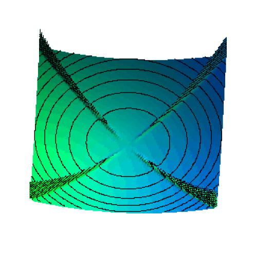
Figure 5: The leading order potential $V_{leading}$

$$V_{\rm leading}=\frac{1}{2}(x^{2}y^{2}+x^{2}z^{2}+\cos^{2}\phi D(y,z))$$

To get rid of the last term scaling analysis in terms of $R$ is not enough. Rather, again, we should think of $x$ as being large and constant over typical time-scales of the $(y,z)$ dynamics. After a last change of variables to

$$y=r\sin\psi,\qquad z=r\cos\psi$$

we find that for generic values the last term is strongly suppressed compared to the harmonic oscillator term. Only if $y$ approaches $\pm z$ it acts as a barrier and flips $\psi$ to $\pi/2-\psi$ while $r$ is not affected. This is a discrete symmetry of the oscillator dynamics and therfore does not influence the time dependence of $r$ which causes the deceleration of $x$ as in the generalized toy model.

Therefore, the analysis of the previous section carries over to the full M(atrix)-Model and we have proved that there are no non-trivial scattering solutions that could describe transversal momentum transfer.

4 Instanton tunneling

In the previous section, we have seen that momentum transfer is not possible classically in the matrix model. Thus, one cannot, quantum mechanically, perform a fluctuation analysis around a classical solution. Nevertheless, it might be that genuine non-perturbative quantum processes exist that nevertheless have finite probabilities for processes with different in and out states. In this case, momentum transfer should be viewed as a tunneling process although there is no potential well that forbids the transition classically.

In this section, we are going to calculate a WKB transition probability for such a process. For simplicity, we restrict our attention again to the toy model. We perform a Wick rotation to the Euclidean domain that amounts to flipping the sign of the potential energy. Instead of four valleys we have now four basins that are not bounded from below. Those are separated by two crossing wells along the coordinate axes that have their top at potential energy zero.

In this energy landscape, one expects a motion that asymptotically comes in from the positive $x$-axis then deviates into the north-east basin in a way the down-hill force is balanced by the centrifugal force and then leaves asymptotically along the positive $y$ axis. There is a simple argument that such a solution has to exist: Take the particle to be on the line $x=y$ at some instant of time with a velocity vector

$$(\dot{x},\dot{y})=(-v,v).$$ (5)

For small values of $v$, the motion is not fast enough to go over the wall along the $y$-axis and the particle will end up in the north-east basin while for large values of $v$ the motion will overshoot the wall along the $y$-axis and the particle will roll down the north-west basin.

By continuity, there must be a value to which $v$ can be fine-tuned such that it will just make it asymptotically to the top of the $y$-axis wall. Using time reversal symmetry together with $x\leftrightarrow y$ one finds that for this solution also comes asymptotically from the top of the $x$-axis.

Note that after fixing the critical value of $v$ also the asymptotic velocities $v_{\infty}$ are determined by energy conservation. The only free parameter is the point where the particle crosses the line $x=y$. This remaining freedom comes from the scaling symmetry

$$(x,y)\mapsto\lambda(x,y),\qquad t\mapsto\lambda^{-1}t,\qquad{\cal S}\mapsto\lambda^{3}{\cal S}$$

of the model. Using this symmetry one finds a one to one correspondence between asymptotic velocities and crossing points on $x=y$.

The only assumption we made about the orbit was 5. Dropping this, it is highly unlikely that further solutions exist since for any other direction of the initial velocity one would still have only one parameter to tune (the magnitude of the velocity) but fine-tuning the final direction to be along the top of the wall $x=0$ would destroy the fine-tuning for $t\to-\infty$. Therefore the symmetric choice is the only possibility to achieve $y\to 0$ initially and $x\to 0$ for late times due to the instability of the potential.

Since there is not much hope to find the critical solution analytically, we have used mathematica to determine it numerically.

Figure 6: The numerical solution with $v=v_{\rm crit}$

We found

$$v_{\rm crit}=1.5099906769x_{0}^{2}$$

where $(x_{0},x_{0})$ is the initial point on the line $x=y$. The leading order of the quantum mechanical probability for this amplitude is given by the classical action of the orbit. As the initial and final velocities $v_{\infty}$ do not vanish, the action is infinite. But so is the action for the trivial solution. Thus we can calculate the difference between these two actions yielding a relative probability:

$$\frac{p({\rm trivial})}{p({\rm tunnel})}=e^{-({\cal S}_{\rm trivial}-{\cal S}_{\rm tunnel})},$$

where the difference of the actions is given by

$${\cal S}_{\rm trivial}-{\cal S}_{\rm tunnel}=\int_{-\infty}^{\infty}\!\!\!dt\,\frac{1}{2}(v_{\infty}^{2}-\dot{x}^{2}-\dot{y}^{2}+x^{2}y^{2})=1.12x_{0}^{3}$$

where the integral again has been evaluated numerically.

The integrand falls off exponentially with $|t|\to\infty$. Therefore, it is no problem to perform the integration only for those values of $t$ for which the numerics of the solution are stable (given the instability of the euclidian potential).

5 Conclusions

In this note, we have shown that there are no non-trivial scattering solutions in the M(atrix)-Model. Therefore it is classically impossible to study processes in which transversal momentum is transferred between the two partons. This is quite different compared to what is known about the 1+1-dimensional case of M(atrix)-String-Theory. There, such solutions have been constructed.

As the M(atrix)-Model and M(atrix)-String-Theory are only equivalent (via T-duality) in the $N\to\infty$ limit, these findings cast further doubt on the usefulness of the finite $N$ version of the M(atrix)-Model-conjecture of [2]. Rather it seems there are quite strong dynamical restrictions on the super-gravity kinematics that this model is able to describe.

The result can also be formulated reversely: Among all classical orbits of the M(atrix)-Model equations of motion only a zero-set (namely the trivial solutions) are scattering solutions whereas all possible other ones are bound solutions that cannot get away from the stadium.

On the other hand, this is quite a welcome behavior for the super-membrane interpretation[24] of the M(atrix)-Model: There, what are scattering solutions from the D0-particle perspective are degenerate solutions for which for early and late times all the energy of the membrane is in the infinite growth of a single mode of the world-volume coordinates. The bound solutions are more like what one would expect of a fluctuating membrane.

- [1] T. Banks, W. Fischler, S. H. Shenker, and L. Susskind, M-theory as a matrix model: A conjecture, Phys. Rev. D55 (1997) 5112–5128, [hep-th/9610043].
- [2] L. Susskind, Another conjecture about m(atrix) theory, hep-th/97040 80.
- [3] M. R. Douglas, D. Kabat, P. Pouliot, and S. H. Shenker, D-branes and short distances in string theory, Nucl. Phys. B485 (1997) 85–127, [hep-th/9608024].
- [4] K. Becker and M. Becker, A two loop test of M(atrix) theory, Nucl. Phys. B506 (1997) 48, [hep-th/9705091].
- [5] K. Becker, M. Becker, J. Polchinski, and A. Tseytlin, Higher order graviton scattering in M(atrix) theory, Phys. Rev. D56 (1997) 3174–3178, [hep-th/9706072].
- [6] P. Kraus, Spin-orbit interaction from matrix theory, Phys. Lett. B419 (1998) 73, [hep-th/9709199].
- [7] I. N. McArthur, Higher order spin-dependent terms in d0-brane scattering from the matrix model, Nucl. Phys. B534 (1998) 183, [hep-th/9806082].
- [8] M. Barrio, R. Helling, and G. Polhemus, Spin-spin interaction in matrix theory, JHEP 05 (1998) 012, [hep-th/9801189].
- [9] W. T. IV and M. V. Raamsdonk, Three-graviton scattering in matrix theory revisited, Phys. Lett. B438 (1998) 248, [hep-th/9806066].
- [10] Y. Okawa and T. Yoneya, Multi-body interactions of d-particles in supergravity and matrix theory, Nucl. Phys. B538 (1999) 67, [hep-th/9806108].
- [11] J. C. Plefka, M. Serone, and A. K. Waldron, The matrix theory s-matrix, Phys. Rev. Lett. 81 (1998) 2866–2869, [hep-th/9806081].
- [12] S. Hyun, Y. Kiem, and H. Shin, Supersymmetric completion of supersymmetric quantum mechanics, Nucl. Phys. B558 (1999) 349, [hep-th/9903022].
- [13] S. Paban, S. Sethi, and M. Stern, Constraints from extended supersymmetry in quantum mechanics, Nucl. Phys. B534 (1998) 137, [hep-th/9805018].
- [14] H. Nicolai and J. Plefka, A note on the supersymmetric effective action of matrix theory, hep-th/0001106.
- [15] R. Helling, J. Plefka, M. Serone, and A. Waldron, Three graviton scattering in m-theory, Nucl. Phys. B559 (1999) 184–204, [hep-th/9905183].
- [16] E. Witten, String theory dynamics in various dimensions, Nucl. Phys. B443 (1995) 85–126, [hep-th/9503124].
- [17] R. Dijkgraaf, E. Verlinde, and H. Verlinde, Matrix string theory, Nucl. Phys. B500 (1997) 43, [hep-th/9703030].
- [18] S. B. Giddings, F. Hacquebord, and H. Verlinde, High energy scattering and d-pair creation in matrix string theory, Nucl. Phys. B537 (1999) 260, [hep-th/9804121].
- [19] G. E. Arutyunov and S. A. Frolov, Virasoro amplitude from the s(n) r**24 orbifold sigma model, Theor. Math. Phys. 114 (1998) 43, [hep-th/9708129].
- [20] G. E. Arutyunov and S. A. Frolov, Four graviton scattering amplitude from s(n) r**8 supersymmetric orbifold sigma model, Nucl. Phys. B524 (1998) 159, [hep-th/9712061].
- [21] B. de Wit, M. Lüscher, and H. Nicolai, The supermembrane is unstable, Nucl. Phys. B320 (1989) 135.
- [22] S. Sethi and M. Stern, D-brane bound states redux, Commun. Math. Phys. 194 (1998) 675, [hep-th/9705046].
- [23] B. Dahmen and B. Raabe, Unconstrained and yang-mills classical mechanics, Nucl. Phys. B384 (1992) 352.
- [24] B. de Wit, J. Hoppe, and H. Nicolai, On the quantum mechanics of supermembranes, Nucl. Phys. B305 (1988) 545.