SUMMATION AND RENORMALIZATION OF BUBBLE GRAPHS TO ALL ORDERS

Abstract

We introduce the 2PPI expansion which sums the bubble graphs to all orders. We show that this expansion can be renormalised with the usual counterterms in a mass independent scheme. We discuss its application to the O(N) linear $\sigma$-model.

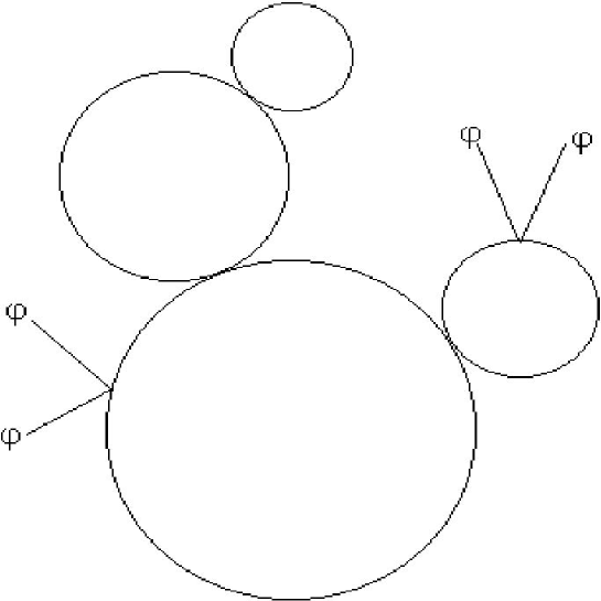
Figure 1: Generic 2PPR diagram

Over the years, the summation of bubble graphs has attracted a lot of interest because of the need to resort to non-perturbative approaches in quantum field theory at finite temperature [1]. In het O(N) linear $\sigma$-model, bubble graphs were originally [2] summed using the $N\rightarrow\infty$ approach. For finite N, it took some while to overcome combinatorial problems [3], but finally consistent results were obtained in [4,5], using the CJT [6] formalism. There were still some problems though with renormalization which could only be implemented consistently in the $N\rightarrow\infty$ limit.
In this letter we discuss the 2PPI expansion which we introduced in [7], as an approximation scheme for calculating the effective potential of the local composite operator $\phi^{2}$. It resembles the 2PI expansion or CJT-method, in that it restricts the topology of the Feynman diagrams at the cost of introducing a selfconsistency condition. In contradistinction to the 2PI expansion, the self consistency equation (gap equation) is local for the 2PPI expansion. First, we will rederive the 2PPI expansion in a new way which makes the renormalization proof more transparent. Then we will show that the usual counterterms renormalize the 2PPI expansion when using a mass independent scheme. Next we calculate the one loop renormalised 2PPI result for the effective potential in the O(N) linear $\sigma$-model and show that it yields the renormalised sum of daisy and superdaisy graphs. Finally we discuss the renormalization problems encountered in previous treatments and show how they are neatly solved in the 2PPI approach.
We will introduce the unrenormalized 2PPI expansion using the $\lambda\phi^{4}$ theory for simplicity. Generalization to the O(N) linear $\sigma$-model is straightforward. We start from the 1PI expansion and try to sum all seagull and bubble graphs exactly. These insertions arise in 2PPR or two particle point reducible graphs because they disconnect from the rest of the diagram when two lines meeting at the same point (the 2PPR-point) are cut (fig.1). We notice that the seagull and bubble graphs contribute to the self energy as effective masses $\frac{\lambda}{2}\varphi^{2}$ and $\frac{\lambda}{2}\langle\phi^{2}\rangle_{c}=\frac{\lambda}{2}\Delta$ respectively. Therefore, we could try to sum all 2PPR insertions by simply deleting the 2PPR graphs from the 1PI expansion and introducing the effective mass :

$$\overline{m}^{2}=m^{2}+\frac{\lambda}{2}(\varphi^{2}+\Delta)$$ (1)

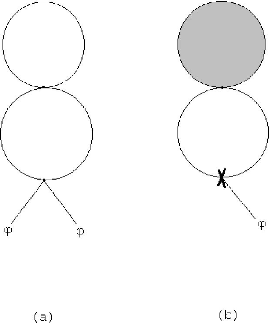
Figure 2: 2PPR part is shaded, 2PPI rest is earmarked

in the remaining 2PPI graphs. This is too naive though since there is a double counting problem which can be easily understood in the simple case of a 2loop vacuum diagram (daisy graph with two petals) of fig. 2.a. Each petal can be seen as a selfenergy insertion in the other, so there is no way of distinguishing one or the other as the remaining 2PPI part. We could however earmark one of the petals by applying a derivative with respect to $\varphi$ (fig. 2.b). This way the 2PPI remainder (which contains the earmark) is uniquely fixed. Now, there are two ways in which the derivative can hit a $\varphi$ field. It can hit an explicit $\varphi$ field which is not a wing of a seagull or it can hit a wing of a seagull or implicit $\varphi$ field hidden in the effective mass. We therefore have :

$$\frac{\delta}{\delta\varphi}\Gamma_{q}^{1PI}(m^{2},\varphi) = \frac{\partial}{\partial\varphi}\Gamma_{q}^{2PPI}(\overline{m}^{2},\varphi)$$ (2)

$$+ \lambda\varphi\frac{\partial}{\partial\overline{m}^{2}}\Gamma^{2PPI}_{q}(\overline{m}^{2},\varphi)$$

where $\Gamma^{1PI}=S(\varphi)+\Gamma_{q}^{1PI}$ or using (1) :

$$\frac{\delta}{\delta\varphi}\Gamma_{q}^{1PI}(m^{2},\varphi)=\frac{\delta}{\delta\varphi}\Gamma_{q}^{2PPI}(\overline{m}^{2},\varphi)-\frac{\lambda}{2}\frac{\delta\Delta}{\delta\varphi}\frac{\partial\Gamma^{2PPI}_{q}}{\partial\overline{m}^{2}}(\overline{m}^{2},\varphi)$$ (3)

Using an analogous combinatorial argument, we have :

$$\frac{\partial\Gamma^{1PI}_{q}}{\partial m^{2}}(m^{2},\varphi)=\frac{\partial\Gamma^{2PPI}_{q}}{\partial\overline{m}^{2}}(\overline{m}^{2},\varphi)$$ (4)

and since $\Delta/2=\frac{\partial\Gamma_{q}^{1PI}}{\partial m^{2}}$ we find the following gap equation for $\Delta$ :

$$\frac{\Delta}{2}=\frac{\partial\Gamma^{2PPI}_{q}}{\partial\overline{m}^{2}}(\overline{m}^{2},\varphi)$$ (5)

The gap equation (5) can be used to integrate (3) and we finally obtain :

$$\Gamma^{1PI}(m^{2},\varphi)=S(\varphi)+\Gamma^{2PPI}_{q}(m^{2}+\frac{\lambda}{2}(\varphi^{2}+\Delta),\varphi)-\frac{\lambda}{8}\int d^{D}x\Delta^{2}$$ (6)

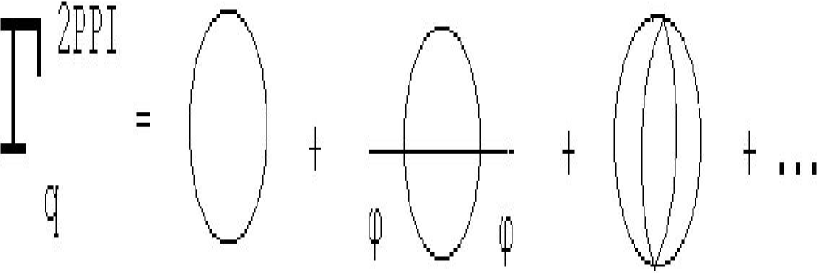
Figure 3: First terms of 2PPI expansion

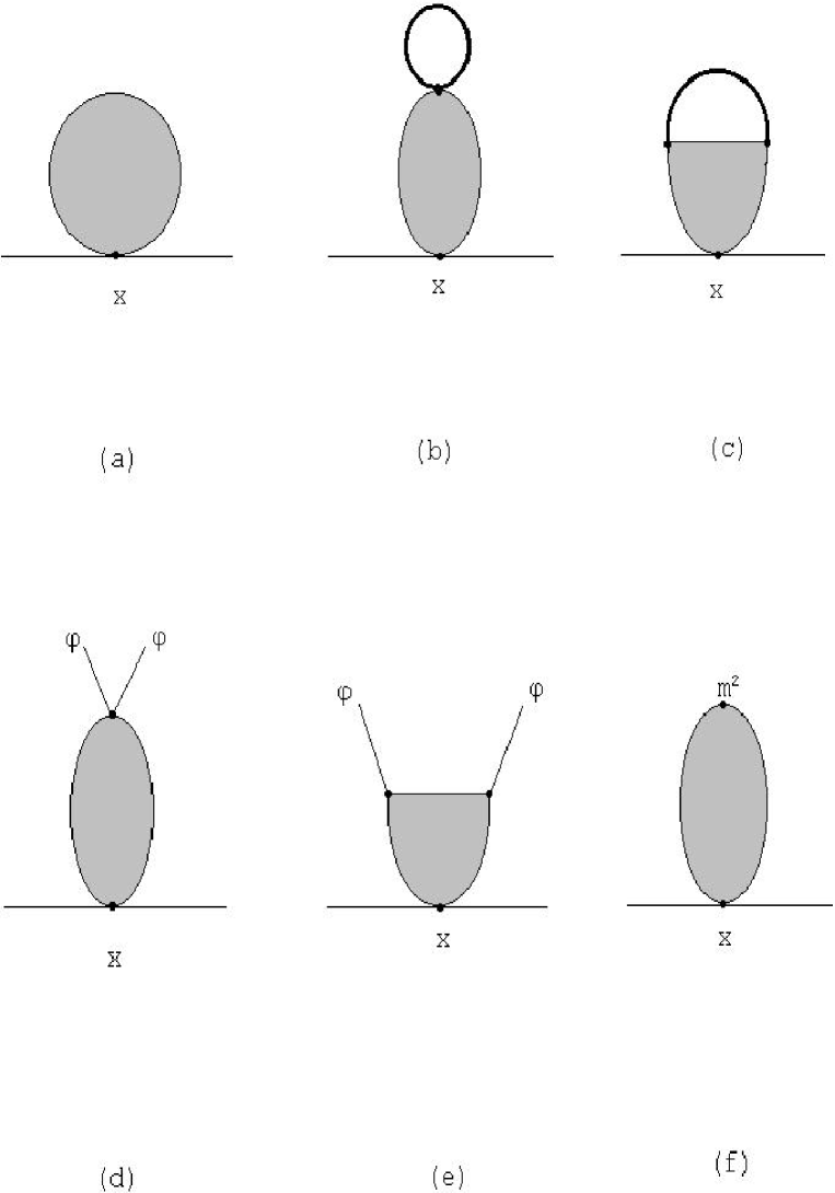
Figure 4: Generic bubble(shaded) and its subdivergences(shaded).Thick lines are full propagators.

This equation together with the gapequation (5) sums the seagulls and bubbles to all orders. The first few diagrams of the 2PPI expansion are displayed in fig.3.
To be useful, we have to show that equation (6) which relates 1PI and 2PPI expansions can be renormalised. Again, we earmark the 1PI diagrams by applying a $\varphi$ derivative so that 2PPR and 2PPI parts are unambiguous. We first renormalize the bubble subgraphs. Consider a generic bubble inserted at the 2PPR point x (fig. 4.a). All primitively divergent subgraphs of the bubble graph which do not contain the 2PPR point x can be renormalised with the counterterms of the $\lambda\phi^{4}$ Lagrangian :

$$\delta{\cal L}=\frac{\delta Z}{2}(\partial_{\mu}\phi)^{2}+\delta Z_{2}\frac{m^{2}\phi^{2}}{2}+\delta Z_{\lambda}\frac{\lambda\phi^{4}}{4!}$$ (7)

As a consequence of these substractions, the contribution of the bubbles to the effective mass is $\frac{\lambda}{2}\langle\phi^{2}\rangle_{c}$ where the connected V.E.V. is now calculated with the full Lagrangian, counterterms included. For subgraphs of the bubble containing the 2PPR point, we need only the 2PPR-parts of the counterterms. Let’s first renormalise the proper subgraphs of the bubble which contain x. Their generic topology is displayed in fig. 4.b and fig. 4.c. They can be made finite with the 2PPR part $\delta Z_{\lambda}^{2PPR}\lambda\phi^{4}/4!$ and contribute $\frac{\lambda}{2}\delta Z^{2PPR}_{\lambda}\langle\phi^{2}\rangle_{c}$ to the effective mass. We still have to subtract the overall divergences of the bubble graph. Their generic topology is displayed in fig. 4.d and 4.e for coupling constant renormalization and fig. 4.f for mass renormalization. Again only the 2PPR parts of the counterterms have to be used and the subtraction of the overall divergences contributes $\frac{\lambda}{2}\delta Z^{2PPR}_{\lambda}\varphi^{2}+\delta Z_{2}^{2PPR}m^{2}$ to the effective mass. Because we use mass independent renormalisation the 2PPR-part of coupling constant renormalisation $\delta Z^{2PPR}_{\lambda}$ can be related to mass renormalisation $\delta Z_{2}$. Indeed, the divergent parts of the subgraphs in fig. 4.d and 4.e which are of the coupling constant type can be viewed as divergent mass renormalizations with a mass insertion at the 2PPR point $x$ and the $\varphi$ legs as incoming and outgoing legs of the selfenergy graph. Because we use a mass independent renormalization scheme (for example minimal substration), not only the divergent parts but also the finite parts of the corresponding counterterms can be chosen equal so that we have

$$\delta Z^{2PPR}_{\lambda}=\delta Z_{2}$$ (8)

Adding the various contributions coming from renormalising the bubble graphs, we find for the renormalised effective mass :

$$\overline{m}^{2}_{R}=m^{2}\left(1+\delta Z_{2}^{2PPR}\right)+\frac{\lambda}{2}\left(1+\delta Z_{\lambda}^{2PPR}\right)(\varphi^{2}+\Delta)$$ (9)

where $\Delta=\langle\phi^{2}\rangle_{c}$ or using (8) :

$$\overline{m}^{2}_{R}=m^{2}+\frac{\lambda}{2}\left(Z_{2}(\varphi^{2}+\Delta)+\frac{2\delta Z^{2PPR}_{2}}{\lambda}m^{2}\right)$$ (10)

We can rewrite this as :

$$\overline{m}^{2}_{R}=m^{2}+\frac{\lambda}{2}(\varphi^{2}+\Delta_{R})$$ (11)

where we have introduced the renormalised V.E.V. of the composite operator $\phi^{2}$ :

$$\langle\phi^{2}\rangle_{c,R}=\Delta_{R}=Z_{2}\Delta+\delta Z_{2}\varphi^{2}+\frac{2\delta Z^{2PPR}_{2}}{\lambda}m^{2}$$ (12)

After renormalizing the bubble subgraphs, the $\varphi$ derivative of $\Gamma^{1PI}_{q}$ can be written as :

$$\frac{\delta}{\delta\varphi}\Gamma^{1PI}_{q,BR}(m^{2},\varphi)=\frac{\partial}{\partial\varphi}\Gamma^{2PPI}_{q}(\overline{m}^{2}_{R},\varphi)+\lambda\varphi\frac{\partial}{\partial\overline{m}^{2}_{R}}\Gamma_{q}^{2PPI}(\overline{m}^{2}_{R},\varphi)$$ (13)

where BR stands for ”bubble renormalised”.
Because there is no overlap, having renormalised the bubbles, we can now renormalize the 2PPI remainder (which contains the earmarked vertex). Let us first consider mass renormalization. A subgraph $\gamma$ in the 2PPI remainder of $\frac{\delta}{\delta\varphi}\Gamma^{1PI}_{q,BR}$ that needs mass renormalization can be made finite with a counterterm $\delta Z_{2}(\gamma)m^{2}\phi^{2}/2$. However, for any such subgraph $\gamma$, there are subgraphs $\gamma^{\prime}$ obtained from $\gamma$ by replacing the mass $m^{2}$ with a seagull or renormalised bubble. These subgraphs require coupling constant renormalization which entails an effective counterterm $\delta Z^{2PPR}_{\lambda}(\gamma^{\prime})(\frac{\lambda}{2}\varphi^{2}+\frac{\lambda}{2}\Delta_{R})\phi^{2}/2$. Taking into account the identity of the renormalization constants for mass and 2PPR-coupling constant renormalization (eq.8), the counterms for these mass-type divergent subgraphs of $\frac{\delta\Gamma^{1PI}_{q,BR}}{\delta\varphi}$ add up to $\delta Z_{2}(\gamma)\overline{m}^{2}_{R}\phi^{2}/2$, exactly what is needed for mass renormalization of $\Gamma^{2PPI}_{q}(\overline{m}^{2}_{R},\varphi)$ in the right hand side of equation (13). The remaining divergent subgraphs need wavefunction renormalization or are of the coupling constant renormalization type that cannot be generated by inserting seagulls or bubbles in a mass-type divergent subgraph. They are made finite by counterterms independent of mass and hence are the same for left and right hand sides of equation (13). Therefore, we can conclude that in a mass independent renormalization scheme, equation (2) can be renormalised with the available counterterms as :

$$\frac{\delta}{\delta\varphi}\Gamma^{1PI}_{q,R}(m^{2},\varphi)=\frac{\partial}{\partial\varphi}\Gamma^{2PPI}_{q,R}(\overline{m}^{2}_{R},\varphi)+\lambda\varphi\frac{\partial}{\partial\overline{m}^{2}_{R}}\Gamma^{2PPI}_{q,R}(\overline{m}^{2}_{R},\varphi)$$ (14)

To proceed, we have to renormalise the gap equation (eq.4). Using essentially the same arguments as in the previous paragraphs, we find that

$$\frac{\partial\Gamma^{1PI}_{q,R}}{\partial m^{2}}(m^{2},\varphi)=\frac{\partial\Gamma^{2PPI}_{q,R}}{\partial\overline{m}^{2}_{R}}(\overline{m}^{2}_{R},\varphi)$$ (15)

From the pathintegral we readily obtain

$$\frac{\partial\Gamma^{1PI}_{R}}{\partial m^{2}}(m^{2},\varphi)=\frac{1}{2}Z_{2}(\varphi^{2}+\langle\phi^{2}\rangle_{c})+\frac{\partial}{\partial m^{2}}(\delta E_{vac})$$ (16)

where $\delta E_{vac}$ is the counterterm needed to cancel divergences in the vacuum energy. In dimensional regularisation, one can easily show that $\delta E_{vac}=\frac{m^{4}}{2}\delta\zeta$, where $\delta\zeta$ is the logarithmically divergent part of $\langle\phi^{2}(x)\phi^{2}(y)\rangle$ which, up to finite parts, is equal to $\frac{\delta Z^{2PPR}_{2}}{\lambda}$. In a mass independent renormalization scheme, finite renormalization can be chosen so that

$$\delta E_{vac}=\frac{m^{4}}{2\lambda}\delta Z^{2PPR}_{2}$$ (17)

Using $\frac{\partial}{\partial m^{2}}\Gamma^{1PI}_{R}=\varphi^{2}/2+\frac{\partial}{\partial m^{2}}\Gamma^{1PI}_{q,R}$ and equations (15), (16) and (17) we obtain

$$\frac{1}{2}\left(Z_{2}\langle\phi^{2}\rangle_{c}+\delta Z_{2}\varphi^{2}+2m^{2}\frac{\delta Z_{2}^{2PPR}}{\lambda}\right)=\frac{\partial\Gamma^{2PPI}_{q,R}}{\partial\overline{m}^{2}_{R}}(\overline{m}^{2}_{R},\varphi)$$ (18)

which because of equation (12) can be written as the renormalised gap equation :

$$\frac{\Delta_{R}}{2}=\frac{\partial\Gamma^{2PPI}_{q,R}}{\partial\overline{m}^{2}_{R}}(\overline{m}^{2}_{R},\varphi)$$ (19)

As in the unrenormalised case (cfr. eq.3), this gapequation can be used to integrate equation (14) and we finally arrive at :

$$\Gamma^{1PI}_{R}(m^{2},\varphi)=S(\varphi)+\Gamma^{2PPI}_{q,R}\left(m^{2}+\frac{\lambda}{2}(\varphi^{2}+\Delta_{R}),\varphi\right)-\frac{\lambda}{8}\int d^{D}x\Delta^{2}_{R}$$ (20)

This equation together with the gapequation (19) sums the seagulls and renormalised bubbles to all orders. To renormalize $\Gamma^{1PI}$, it is therefore sufficient to renormalize $\Gamma^{2PPI}$ using a mass independent renormalisation scheme (MS for example), calculate the renormalised bubble $\Delta_{R}$ from the gapequation and substitute in eq.(20).
The preceding results can be easily generalised to the O(N) linear $\sigma$-model with Lagrangian :

$${\cal L}=\frac{1}{2}\partial_{\mu}\phi_{i}\partial_{\mu}\phi_{i}+\frac{m^{2}_{ij}}{2}\phi_{i}\phi_{j}+\frac{\lambda}{8}(\phi_{ii})^{2}$$ (21)

Seagulls and bubbles can be included in an effective mass

$$\overline{m}^{2}_{ij}=m^{2}_{ij}+\lambda[\varphi_{i}\varphi_{j}+\Delta_{ij}]+\frac{\lambda}{2}[\varphi^{2}+\Delta_{kk}]\delta_{ij}$$ (22)

where $\Delta_{ij}=\langle\phi_{i}\phi_{j}\rangle_{c}$. For the O(N)-linear $\sigma$-model, equations (2) and (3) become :

$$\frac{\delta}{\delta\varphi_{k}}\Gamma^{1PI}_{q}(m^{2},\varphi) = \frac{\partial}{\partial\varphi_{k}}\Gamma^{2PPI}_{q}(\overline{m}^{2},\varphi)+[\lambda\varphi_{k}\delta_{ij}+\lambda(\delta_{ik}\varphi_{j}+\delta_{jk}\varphi_{i})]\frac{\partial\Gamma^{2PPI}_{q}}{\partial\overline{m}^{2}_{ij}}(\overline{m}^{2},\varphi)$$ (23)

$$= \frac{\delta}{\delta\varphi_{k}}\Gamma^{2PPI}_{q}(\overline{m}^{2},\varphi)-\left[\lambda\frac{\delta\Delta_{ij}}{\delta\varphi_{k}}+\frac{\lambda}{2}\delta_{ij}\frac{\delta\Delta_{ll}}{\delta\varphi_{k}}\right]\frac{\partial\Gamma^{2PPI}_{q}}{\partial\overline{m}^{2}_{ij}}(\overline{m}^{2},\varphi)$$

We can use the gapequation $\Delta_{ij}/2=\frac{\partial\Gamma^{2PPI}}{\partial\overline{m}^{2}_{ij}}(\overline{m}^{2},\varphi)$ to integrate the last equation and obtain :

$$\Gamma^{1PI}(m^{2},\varphi)=S(\varphi)+\Gamma^{2PPI}_{q}(\overline{m}^{2},\varphi)-\frac{\lambda}{8}\int d^{D}x\left[(\Delta_{ii})^{2}+2(\Delta_{ij})^{2}\right]$$ (24)

For $m^{2}_{ij}=\delta_{ij}m^{2}$, we can make use of O(N) symmetry to define :

$$\overline{m}^{2}_{ij}=\frac{\varphi_{i}\varphi_{j}}{\varphi^{2}}\overline{m}^{2}_{\sigma}+\left(\delta_{ij}-\frac{\varphi_{i}\varphi_{j}}{\varphi^{2}}\right)\overline{m}^{2}_{\pi}$$ (25)

and

$$\Delta_{ij}=\frac{\varphi_{i}\varphi_{j}}{\varphi^{2}}\Delta_{\sigma}+\left(\delta_{ij}-\frac{\varphi_{i}\varphi_{j}}{\varphi^{2}}\right)\Delta_{\pi}$$ (26)

so that because of (22) :

$$\overline{m}^{2}_{\sigma} = m^{2}+\frac{3\lambda}{2}\left[\varphi^{2}+\Delta_{\sigma}+\frac{N-1}{3}\Delta_{\pi}\right]$$

$$\overline{m}^{2}_{\pi} = m^{2}+\frac{\lambda}{2}\left[\varphi^{2}+\Delta_{\sigma}+(N+1)\Delta_{\pi}\right]$$ (27)

The relation between 1PI and 2PPI expansion now simplifies to

$$\Gamma^{1PI}(m^{2},\varphi) = S(\varphi)+\Gamma^{2PPI}_{q}(\overline{m}^{2}_{\sigma},\overline{m}^{2}_{\pi},\varphi)$$ (28)

$$- \frac{\lambda}{8}\int d^{D}x\left[3\Delta^{2}_{\sigma}+(N^{2}-1)\Delta^{2}_{\pi}+2(N-1)\Delta_{\sigma}\Delta_{\pi}\right]$$

and the gap equations are

$$\frac{\delta\Gamma^{2PPI}}{\delta\overline{m}^{2}_{\sigma}} = \frac{\Delta_{\sigma}}{2}$$

$$\frac{\delta\Gamma^{2PPI}}{\delta\overline{m}^{2}_{\pi}} = (N-1)\frac{\Delta_{\pi}}{2}$$ (29)

To show the efficiency of the 2PPI expansion, let’s calculate the effective potential at one loop 2PPI. We choose $\varphi_{i}=\delta_{iN}\varphi$. Since there are $(N-1)$ masses $\overline{m}_{\pi}$, and one mass $\overline{m}_{\sigma}$ running in the loop, we have :

$$V^{2PPI}_{q}(\overline{m}^{2}_{\sigma},\overline{m}^{2}_{\pi},\varphi)=\frac{1}{2}\int\frac{d^{D}p}{(2\pi)^{D}}\ln(p^{2}+\overline{m}^{2}_{\sigma})+\frac{(N-1)}{2}\int\frac{d^{D}p}{(2\pi)^{D}}\ln(p^{2}+\overline{m}^{2}_{\pi})$$ (30)

The renormalization procedure of $\Gamma^{1PI}$ is completely analogous as in the $N=1$ case (for details, see [8]). We can simply renormalize $\Gamma^{2PPI}$ using for example the $\overline{MS}$ scheme and calculate the renormalised bubbles $\Delta_{\sigma,R}$ and $\Delta_{\pi,R}$ by using the renormalised gapequations (29). We finally obtain at one loop 2PPI :

$$V_{R}^{1PI}(m^{2},\varphi) = V(\varphi)+\frac{\overline{m}^{4}_{\sigma,R}}{64\pi^{2}}\left[\ln\frac{\overline{m}^{2}_{\sigma,R}}{\overline{\mu}^{2}}-\frac{3}{2}\right]+(N-1)\frac{\overline{m}^{4}_{\pi,R}}{64\pi^{2}}\left[\ln\frac{\overline{m}^{2}_{\pi,R}}{\overline{\mu}^{2}}-\frac{3}{2}\right]$$ (31)

$$- \frac{\lambda}{8}\left[3\Delta^{2}_{\sigma,R}+(N^{2}-1)\Delta^{2}_{\pi,R}+2(N-1)\Delta_{\sigma,R}\Delta_{\pi,R}\right]$$

where

$$\Delta_{\ast,R}=\frac{\overline{m}^{2}_{\ast,R}}{16\pi^{2}}\left[\ln\frac{\overline{m}^{2}_{\ast,R}}{\overline{\mu}^{2}}-1\right]$$ (32)

and $\overline{m}_{\sigma,R}$ and $\overline{m}_{\pi,R}$ are given by equation (27) with renormalised $\Delta^{\prime}s$.
From the topology of the one loop 2PPI graph, it is clear that our 1loop 2PPI result agrees with the Hartree approximation and should give the sum of daisy and superdaisy graphs. If we compare our unrenormalised expression we find complete agreement (after some algebra) with the unrenormalised sum of daisy and superdaisy graphs published in [4,5] and [9] and obtained within the CJT formalism [6] (2PI expansion). The advantage of our 2PPI expansion is that we quite naturally obtain a simple expression by keeping only the one loop 2PPI vacuum bubble, while in the 2PI approach one has to keep part of the 2loop graphs (the O($\lambda$) part) and the simple expression (31) is only obtained after some rearrangement. Furthermore, one can easily calculate higher order terms in the 2PPI expansion while in the 2PI expansion, it is very difficult to go beyond the Hartree approximation because of the non-locality of the gap equations. Concerning renormalization, we find complete agreement with the renormalised expression of [9] obtained using the auxiliary field method. We disagree with the ”non-perturbative” renormalisation used in [4,5]. These authors find that in order to obtain a finite effective mass (which sums daisy and superdaisy graphs), the coupling constant has to run in a different way than is dictated by the perturbative renormalisation group. For the N=1 case, their non-perturbative $\beta$-function is a factor of three smaller than the perturbative one and is essentially the $N\rightarrow\infty$ $\beta$ function extrapolated to N=1. Our 2PPI analysis to all orders can easily explain this paradox. We showed in (9) that after adding counterterms, the renormalised effective mass can be written as :

$$\overline{m}^{2}_{R}=\left(m^{2PPR}_{0}\right)^{2}+\frac{\lambda^{2PPR}_{0}}{2}(\varphi^{2}+\Delta)$$ (33)

This relation is valid to all orders. At one loop one has $\delta Z^{2PPR}_{2}=\delta Z_{2},\delta Z_{\lambda}^{2PPR}=\frac{1}{3}\delta Z_{\lambda}$. So, if one naively assumes $\lambda_{0}=\lambda_{0}^{2PPR}$, one obtains a $\beta$-function which is a factor of three too small. This factor of three is due to crossing which changes a 2PPR coupling constant renormalisation insertion into a 2PPI one. This also explains why the $N=\infty$ renormalisation is straightforward : crossing terms (and hence Fock or 2PPI terms) are subdominant and only the 2PPR or Hartree terms survive in the $N\rightarrow\infty$ limit.
In summary, we have presented a method for summing and renormalising bubble graph insertions to all orders based on the 2PPI expansion. Besides the O(N) linear $\sigma$-model, also Q.E.D. and models with four-fermion couplings or Yukawa couplings can be treated in this expansion. Finite temperature effects can be easily included. In [9], we sum daisy and superdaisy graphs of O(N) linear $\sigma$-model at finite T, using the 2PPI expansion. Renormalisation is straightforward and the Goldstone theorem is obeyed to all orders. Extension to the non-equilibrium domain is possible [10].

References

• [1] J.I. Kapusta, Finite-temperature field theory (Cambridge University Press,1989)
• [2] L. Dolan and R. Jackiw, Phys.Rev. D 9 (1974) 3320
• [3] J.R. Epinosa, M. Quiros and F. Zwirner, Phys.Lett. B 291 (1992) 115
C.G. Boyd, D.E. Brahm and S.D.H. Hsu, Phys.Rev. D 48 (1993), 4952
C.G. Boyd, D.E. Brahm and S.D.H. Hsu, Phys.Rev. D 48 (1993), 4963
• [4] G. Amelino-Carmelia and S.-Y. Pi, Phys.Rev. D 47 (1993) 2356
• [5] G. Amelino-Carmelia, Phys.Lett. B 407 (1997) 268
• [6] J.M. Cornwall, R. Jackiw and E. Tomboulis, Phys.Rev. D 10 (1974) 2428
• [7] H. Verschelde and M. Coppens, Phys.Lett. B 287 (1992) 133
• [8] J. Depessemier and H. Verschelde, submitted to Phys.Rev. D
• [9] Y. Nemoto, K. Naito and M. Oka, hep-ph/9911431
• [10] H. Verschelde and T. Vanzieleghem, in preparation.
Refer to caption