Abstract
The correlation functions of a two-dimensional rational conformal field theory, for an arbitrary number of bulk and boundary fields and arbitrary world sheets, can be expressed in terms of Wilson graphs in appropriate three-manifolds. We present a systematic approach to boundary conditions that break bulk symmetries. It is based on the construction, by ‘$\alpha$-induction’, of a fusion ring for the boundary fields. Its structure constants are the annulus coefficients and its $6j$-symbols give the OPE of boundary fields. Symmetry breaking boundary conditions correspond to solitonic sectors.

——————
^† Invited talk by Christoph Schweigert at the TMR conference “Non-perturbative quantum effects 2000”, Paris, September 2000; to appear in the Proceedings.

Conformal field theory in two dimensions plays a fundamental role in the theory of two-dimensional critical systems of classical statistical mechanics [1], in quasi one-dimensional condensed matter physics [2] and in string theory [3]. The study of defects in systems of condensed matter physics [4], of percolation probabilities [5] and of (open) string perturbation theory in the background of certain string solitons, the so-called D-branes [6], forces one to analyze conformal field theories on surfaces that may have boundaries and / or can be non-orientable.

In this contribution, we present a systematic description of correlation functions of an arbitrary number of bulk and boundary fields on general surfaces. It is based on the fundamental fact [7, 8] that conformal blocks appear in two different contexts: They are building blocks for the correlators of two-dimensional conformal field theories, and they are the spaces of physical states in topological field theories, TFT, in three dimensions.

For simplicity, we take the modular invariant torus partition function that encodes the spectrum of bulk fields of the theory to be of charge conjugation form, i.e. $Z_{\lambda,\mu}\,{=}\,\delta_{\lambda,\mu^{+}_{\phantom{i}}}$. We will, however, include in our discussion boundary conditions that do not preserve all bulk symmetries. We consider general cases of symmetry breaking by boundary conditions. In particular, we do not have to require that left movers and right movers are linked, at the boundary, by some automorphism of the chiral algebra. Put differently, the subalgebra of chiral symmetries that is preserved by the boundary conditions is not necessarily an orbifold subalgebra. Applications of the theory include non-BPS branes in interacting backgrounds and boundary conditions for exceptional modular invariants.

We will start with a brief review of TFT in three dimensions, and then formulate the basic problem that arises when one constructs a full two-dimensional CFT from a chiral CFT. The amplitudes in the presence of symmetry preserving boundary conditions will be discussed in Section 3. Symmetry breaking boundary conditions are the subject of Section 4.

1 Three-dimensional TFT

The basic feature of three-dimensional TFT is that it provides a modular functor: To geometric data it associates algebraic structures. Concretely, it associates vector spaces – the spaces ${\cal H}(\hat{X})$ of conformal blocks – to two-dimensional manifolds $\hat{X}$, and to three-manifolds, endowed with somewhat more structure, it assigns an endomorphism of these vector spaces.

In thoses cases where the TFT can be defined in terms of path integrals, e.g. for Chern-Simons theories, the reader is invited to think of the vector space ${\cal H}(\hat{X})$ as the space of (gauge equivalence classes of) boundary conditions for the fields appearing in the path integral and to think of the endomorphisms as transition amplitudes. We would like to stress, however, that our approach does not rely on the existence of a path integral description. In fact, the only necessary input is the structure of a modular tensor category [9], which is a formalization of Moore-Seiberg data like fusing and braiding matrices and conformal weights.

More precisely, conformal blocks are associated to extended surfaces: These are two-dimensional, oriented manifolds with a finite collection of small arcs. Each arc carries a label from a set $I$. In our application, these are primary fields, or equivalently, irreducible representations of a chiral symmetry algebra. Moreover, it is necessary to choose a Lagrangian subspace of $H_{1}(\hat{X},{\mathbb{R}})$. We will sometimes suppress these auxiliary data in our discussion.

The endomorphisms are associated to so-called cobordisms $(M,\partial_{-}M,\partial_{+}M)$. Here $M$ is a three-manifold whose boundary $\partial M$ has been decomposed in two disjoint subsets $\partial_{\pm}M$, each of which can be empty. Moreover, a ribbon graph has to be chosen in $M$. After choosing Lagrangian subspaces in $H_{1}(\partial_{\pm}M,{\mathbb{R}})$, the two spaces $\partial_{\pm}M$ become extended surfaces. The endomorphism associated to the cobordism is then a linear map

$$Z(M,\partial_{-}M,\partial_{+}M):\quad{\cal H}(\partial_{-}M)\to{\cal H}(\partial_{+}M)\,.$$

In the application of our interest, we always choose $\partial_{-}M$ to be empty. Using the fact that ${\cal H}(\emptyset)\,{=}\,{\mathbb{C}}\,$, we then obtain a map

$$Z(M,\partial M):\quad{\mathbb{C}}\to{\cal H}(\partial M)\,,$$

in other words, a line in the vector space ${\cal H}(\partial M)$. The image $Z(M,\partial M)1$ of the number 1 under this map then specifies a vector in the vector space ${\cal H}(\partial M)$ of conformal blocks.

Topological field theory thus provides a manageable way to describe explicitly elements in the spaces of conformal blocks, a task that is very difficult in other approaches to these spaces.

2 2-d CFT and chiral blocks

It is important (not only in our present context) to be aware of the fact that the common use of the words “conformal field theory” refers to two rather different types of physical situations. Chiral conformal field theories are defined on oriented manifolds $\hat{X}$ without boundaries. They appear, e.g., in the analysis of the universality class of the edge system of a quantum Hall sample. Indeed, the magnetic field selects a chirality and thereby provides an orientation of the boundary of the sample. The main objects of chiral conformal field theory are the spaces of conformal blocks. It is chiral CFT rather than full conformal field theory that is the boundary theory for a topological field theory.

Full conformal field theory appears in the world sheet formulation of string theory and in the description of universality classes of critical phenomena. It can be defined on surfaces $X$ with boundary and on unoriented surfaces. It is important to realize that even when the surface $X$ is orientable, no orientation is preferred.

Chiral and full CFT are related [10, 11] by a generalization of the mirror trick that is familiar from the treatment of boundaries in classical electrodynamics. Given a surface $X$, one considers the double $\hat{X}$, a surface that is naturally oriented. For example, the double of a disk is the sphere, and the double of a crosscap (the real projective space ${\mathbb{R}}{\mathbb{P}}^{2}$) is a sphere as well. For general surfaces without boundary, the double is the total space of the orientation bundle. In all cases, there is an orientation reversing involution $\sigma{:}\;\hat{X}\to\hat{X}$ such that $X\,{=}\,\hat{X}/\sigma$.

The idea is now to construct correlators for full CFT on $X$ in terms of conformal blocks for the chiral CFT on its double $\hat{X}$ [11]:

The correlators of full CFT on $X$ are specific vectors in the spaces ${\cal H}(\hat{X})$.

The central task of constructing a full CFT from a given chiral CFT is to specify these vectors.

These vectors must obey various consistency constraints. They encode factorization properties as well as locality of the correlation functions as functions of the insertion points and of the moduli of the two-dimensional surface.

To conclude this section, we indicate how this formulation of the problem of constructing a full CFT is related to more conventional descriptions of correlators. If $X$ is closed and orientable, the cover $\hat{X}$ consists of two copies of $X$, but with opposite orientation. Symbolically, $\hat{X}=(+X)\cup(-X)$. Correlators are blocks on $\hat{X}$, and hence bilinear combinations of blocks on $X$.

3 The connecting manifold

Combining the insights outlined in the sections 1 and 2, it is natural to use TFT to describe the vectors in the spaces of conformal blocks that correspond to correlators. More precisely, for every world sheet $X$, we construct [12] a three manifold $M_{X}$ such that its boundary is the double,

$$\partial M_{X}=\hat{X}\,.$$

The manifold $M_{X}$ will be called connecting manifold. For any choice of insertion points on $X$, we will construct a Wilson graph in $M_{X}$ such that

$$Z(M_{X},\hat{X}):\quad{\mathbb{C}}\to{\cal H}(\hat{X})$$

gives the correlator of the full CFT.

Let us start with two examples. When $X$ is the disk, then the double $\hat{X}$ is the sphere $S^{2}$. The orientation-reversing map $\sigma$ is reflection about the equatorial plane. The connecting manifold $M_{X}$ is the full ball. Note that the intervals perpendicular to the equatorial plane provide natural connecting lines between the two pre-images of a bulk point, and that these connections for two different bulk points never intersect. These connecting intervals are a general feature; they motivate the name “connecting manifold”. Our second example is the sphere, $X\,{=}\,S^{2}$, for which the double consists of two disjoint copies of $S^{2}$. The connecting manifold is then the space between two concentric spheres.

In general, $M_{X}$ can be constructed as the total space of an interval bundle over the orientation bundle, seen as a ${\mathbb{Z}}_{2}$-bundle. A contraction over the boundary points ensures that $M_{X}$ is smooth (in this respect $M_{X}$ differs from a similar manifold introduced in [13]).

The next task is to describe the Wilson graph. In this section, we restrict ourselves to boundary conditions that preserve all bulk symmetries. For the topology of the disk our prescription is illustrated in the following picture:

First we join the two pre-images of a bulk point by a Wilson line along the connecting interval. Since we work with the charge conjugation modular invariant, the two insertions on $\hat{X}$ are labelled by conjugate labels $\lambda,\lambda^{+}_{\phantom{|}}$, and we attach to the Wilson line running from the pre-image with $\lambda$ to the preimage labelled with $\lambda^{+}_{\phantom{|}}$ the label $\lambda$.

The components of the boundary $\partial X$ of $X$ correspond to circles on the cover $\hat{X}$. (E.g. in the case of a disk, the single boundary corresponds to the equator of the disk.) In the next step, we put a circular Wilson line ‘close’ to every such boundary circle. The qualification ‘close’ needs some explanation in a topological theory: It means here that none of the Wilson lines for bulk fields runs between the boundary Wilson line and the boundary circle.

The boundary insertions are then joined with little Wilson lines to the corresponding boundary Wilson line. For each boundary insertion this introduces a trivalent vertex. We finally must attach labels to the boundary part of the Wilson graph as well. For the short Wilson lines which join the boundary insertions to the boundary Wilson line, we take the chiral label of the corresponding boundary field. The trivalent vertices partition the circular Wilson line into line segments. To each such segment we must assign a label as well. This label is interpreted as specifying a boundary condition. Indeed, it is known for a long time [14] that under our hypotheses boundary conditions and primary fields are in one-to-one correspondence.

Finally we have to deal with the trivalent vertices. One should assign a coupling to them, i.e. an element in the space of three-point blocks on the sphere. The dimension of that space is given by the fusion rules. Indeed, the partition function for boundary operators $\Psi^{ab}_{\mu}$ is nothing but the annulus amplitude,

$$A_{ab}(t)=\sum_{\nu}A_{ab}^{\nu}\,\chi_{\nu}({\rm i}t/2)\,.$$

Under our hypotheses, the annulus multiplicities $A_{ab}^{\nu}$ are known [14] to be equal to the fusion rules.

We have now specified a Wilson graph in the connecting manifold $M_{X}$ which, according to the general rules, provides us with a specific element in the space of conformal blocks ${\cal H}(\partial M)\,{=}\,{\cal H}(\hat{X})$. This element is the correlator we are looking for:

$$C(X)=Z(M_{X},\hat{X})1\,.$$

(In the present discussion, we have suppressed several technical details like the framing of the Wilson lines or the appropriate choice of Lagrangian subspaces in $H_{1}(\hat{X},{\mathbb{R}})$. All those details can be found in [15].)

Our ansatz provides a description of correlation functions of a conformal field theory in a mathematically rigorous framework (cf. e.g. [9]). As a consequence, we are in a position to prove various theorems about correlation functions. The first statement concerns modular invariance. Consider the group ${\rm Aut}(\hat{X},\sigma)$ of arc-preserving homeomorphisms of $\hat{X}$ of degree 1 that commute with the action of the involution $\sigma$ on $\hat{X}$. When $X$ is the two-torus, this group reduces to the ordinary modular group; in the case of surfaces with boundaries it has been called the relative modular group [16]. One can show that this group acts on the spaces of conformal blocks ${\cal H}(\hat{X})$, that the action is genuine (rather than only projective), and that the correlators are invariant under this action. This establishes modular invariance at all genera.

A second collection of theorems shows that our ansatz is consistent with factorization both in the bulk and on the boundary. At the level of chiral CFT, we have the following structure: Given two arcs in $\hat{X}$, one can cut out little disks around these arcs and glue together the boundaries of the two disks so as to obtain a new surface $\hat{X}^{\prime}$ with two insertion points less. We label the two arcs in $\hat{X}$ by conjugate labels $\lambda,\lambda^{+}_{\phantom{|}}$ and call the corresponding labelled surface $\hat{X}_{\lambda}$. It follows from the axioms of TFT that for each such gluing there is an isomorphism at the level of spaces of conformal blocks:

$$g_{\hat{X}^{\prime},\hat{X}}:\quad\bigoplus_{\lambda}{\cal H}(\hat{X}_{\lambda})\to{\cal H}(\hat{X}^{\prime})\,.$$

The correlation functions are compatible with this structure for the double. On a world sheet $X$ we can glue together two bulk insertions. On the double, this amounts to a simultaneous gluing of two pairs of insertions. For the correlation functions, one finds

$$C(X^{\prime})=\sum_{\lambda}S_{\lambda,\Omega}\,\,g_{\hat{X}^{\prime},\hat{X}}C(X_{\lambda})\,.$$

This is exactly the usual consistency constraint in full CFT, if one takes into account the fact that in our approach the two-point function of bulk fields is normalized to the element $S_{\lambda,\Omega}$ of the modular matrix $S$.

Similarly, one can glue two boundary insertions. In this case, one deals with a single gluing on the double. One finds

$$C(X^{\prime})=\sum_{\lambda}(S_{\lambda,\Omega}/S_{\Omega,\Omega})\,\,g_{\hat{X}^{\prime},\hat{X}}C(X_{\lambda})\circ\gamma\,,$$

which is again compatible with the normalization of the two-point functions of boundary fields. (The map $\gamma$ is a natural contraction on the space of annulus multiplicities.)

Finally one can recover the amplitudes for one bulk insertion on a disk, for three boundary fields on a disk, and for one bulk insertion on the crosscap, as well as the amplitudes for annulus, Klein bottle and Möbius strip. Complete agreement with known results is found.

As an illustrative example, we consider the case of a single bulk insertion $\Phi_{\lambda,\lambda^{+}_{\phantom{I}}}$ on a disk with boundary condition $a$. In this case the space of blocks is one-dimensional. Our task is then to compare the Wilson graph of figure 1 with the standard basis that is displayed in figure 2. (In the present context, this particular conformal block $B(S^{2};\lambda,\lambda^{+}_{\phantom{I}})$ is often called an ‘Ishibashi state’). We now obtain $S^{3}$ by gluing with a single three-ball. When applied to figure 2, we get the unknot with label $\lambda$ in $S^{3}$, for which the link invariant is $S_{0,\lambda}$. In the case of figure 1 we get a pair of linked Wilson lines with labels $a$ and $\lambda$ in $S^{3}$; the value of the link invariant for this graph is $S_{a,\lambda}$.

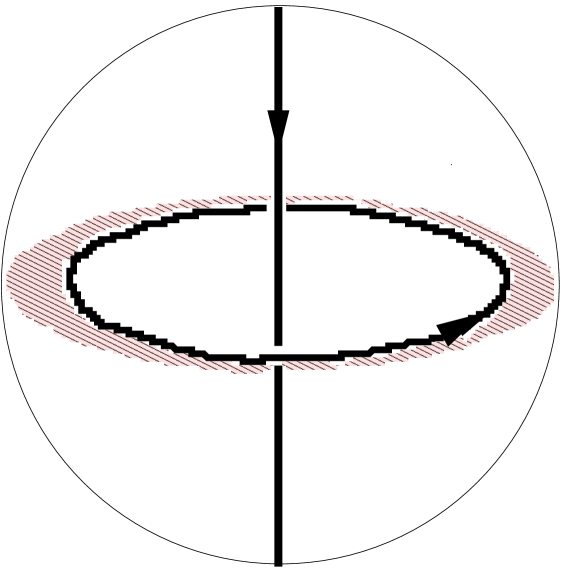
Figure 1: $C(D_{a};\lambda)$

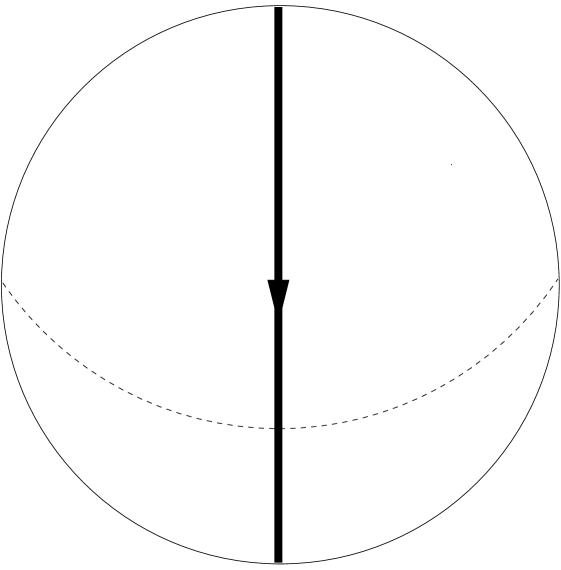
Figure 2: $B(S^{2};\lambda,\lambda^{+})$

Comparison thus shows that the correlation function is $S_{a,\lambda}/S_{0,\lambda}$ times the standard two-point block on the sphere,

$$C(D_{a};\lambda)=(S_{a,\lambda}/S_{0,\lambda})\cdot B(S^{2};\lambda,\lambda^{+}_{\phantom{|}})\,.$$

Taking into account the normalization of bulk fields, we recover the known result that the correlator for a canonically normalized bulk field $\lambda$ on a disk with boundary condition $a$ is $S_{a,\lambda}/\!\sqrt{S_{0,\lambda}}$ times the standard two-point block on the sphere. (This relation forms the basis of the so-called boundary state formalism [14].)

4 Symmetry breaking boundary conditions

We now study the more general case of boundary conditions that break part of the bulk symmetries: We only require that some subalgebra $\bar{\cal A}$ of the algebra ${\cal A}$ of chiral symmetries is preserved by the boundary conditions.

A particularly simple realization of this situation arises when $\bar{\cal A}$ is an orbifold subalgebra of ${\cal A}$: Fix a group $G$ of automorphisms of ${\cal A}$ and define $\bar{\cal A}$ to be the subalgebra of elements of ${\cal A}$ that are left pointwise fixed by all automorphisms in $G$. In case $G$ is a finite abelian group, many aspects of boundary conditions that preserve only $\bar{\cal A}$ are known [17]. The two most important insights in our present context are the following:
   Bulk and boundary fields carry labels from two distinct sets.
   Boundary conditions that break bulk symmetries correspond to twisted representations of the chiral algebra ${\cal A}$.
There is a notion of fusion for such representations [18], and the annulus coefficients can be expected [19, 20] to coincide with the fusion rules of twisted representations.

Together with the observation that in our Wilson graphs bulk and boundary fields always lie in different connected components of a graph, the first point suggests the description in terms of a new fusion ring for the boundary fields. We stress that this fusion ring cannot be expected to be modular. Indeed, for twisted representations the conformal weight does not have the same fractional part for all states in the module, so there is no ‘twist’. Since every braided tensor $*$-category with conjugates automatically has a twist, one cannot expect a braiding either.

We now concentrate on the boundary fusion ring. Its structure constants are the annulus multiplicities. It can be obtained from the fusion ring of the $\bar{\cal A}$-theory by the following general recipe [21]:  The vacuum module ${\cal H}_{\Omega}$ of the ${\cal A}$-theory decomposes into $\bar{\cal A}$-modules with certain multiplicities:

$${\cal H}_{\Omega}=\bigoplus_{\bar{\mu}}n_{\bar{\mu}}\bar{\cal H}_{\bar{\mu}}\,.$$

The non-negative integers $n_{\bar{\mu}}$ define an element $\bar{\theta}$ of the fusion ring of $\bar{\cal A}$:

$$\bar{\theta}=\sum_{\bar{\mu}}n_{\bar{\mu}}\Phi_{\bar{\mu}}\,.$$

To every element $\Phi_{\bar{\lambda}}$ of the fusion ring for $\bar{\cal A}$ one now associates an element $\alpha_{\bar{\lambda}}$ in a new fusion ring ${\cal A}^{\prime}$. This operation preserves multiplication, addition and conjugates:

$$\alpha_{\bar{\lambda}}{\star}\,\alpha_{\bar{\mu}}\,{=}\,\alpha_{\bar{\lambda}\star\bar{\mu}}\,,\ \ \alpha_{\bar{\lambda}}{+}\,\alpha_{\bar{\mu}}\,{=}\,\alpha_{\bar{\lambda}+\bar{\mu}}\,,\ \ {(\alpha_{\bar{\lambda}})}^{+}\,{=}\,\alpha_{\bar{\lambda}}^{+}$$

This would not lead to anything new, were it not for another definition, namely of the spaces of homomorphisms: We set

$${\rm Hom}_{{\cal A}^{\prime}}(\alpha_{\bar{\lambda}},\alpha_{\bar{\mu}}):={\rm Hom}_{\bar{\cal A}}(\Phi_{\bar{\lambda}},\bar{\theta}\star\Phi_{\bar{\mu}})\,.$$

This relation implies that even when $\bar{\lambda}$ is simple, i.e. corresponds to an irreducible representation of the chiral algebra $\bar{\cal A}$, the induced object $\alpha_{\bar{\lambda}}$ is not necessarily simple. It may even happen that the category ${\cal A}^{\prime}$ does not contain enough simple objects to decompose every object into a direct sum of simple objects. This is a generalization of the problem of fixed point resolution in simple current extensions. A general construction in tensor $*$-categories guarantees the existence of a bigger category ${\cal A}_{{\rm bound}}$ in which the fixed points are resolved. Unfortunately, this prescription cannot (yet) be made as explicit as [23] in the simple current case.

We take this resolved tensor category ${\cal A}_{{\rm bound}}$ as the boundary category. Its simple objects correspond to (elementary) boundary conditions. The structure constants in the tensor product correspond to the annulus multiplicities. The sectors actually come in two classes, solitonic or local. Local sectors correspond to symmetry preserving boundary conditions. The solitonic sectors correspond, in the case of simple current extensions, to boundary conditions with non-vanishing monodromy charge, which implies a non-trivial automorphism type (or, equivalently, a non-trivial gluing automorphism on the boundary). More generally, symmetry breaking boundary conditions are in one-to-one correspondence to solitonic representations of the chiral symmetry ${\cal A}$. The resolved tensor category ${\cal A}_{{\rm bound}}$ is associative and closed under subobjects. Thus one can define $6j$-symbols; the same arguments as in the Cardy case [20, 24] then show that the OPE of two boundary fields coincides with these $6j$-symbols. 

To conclude this contribution, let us emphasize that the space of boundary conditions carries a surprising amount of beautiful structure. The presence of this structure makes us confident that many more problems can be tackled than one could have hoped for some time ago.

Acknowledgement:
The results presented in Section 3 have been obtained in collaboration with Giovanni Felder and Jürg Fröhlich. We would like to thank them for a very pleasant collaboration as well as for discussions on the contents of Section 4.

References

- [1] J. Cardy, in: Fields, Strings, and Critical Phenomena (North Holland, Amsterdam 1989), p. 169
- [2] I. Affleck, in: Fields, Strings, and Critical Phenomena (North Holland, Amsterdam 1989), p. 563
- [3] J. Polchinski, String Theory (Cambridge University Press, Cambridge 1998)
- [4] M. Oshikawa and I. Affleck, Nucl. Phys. B 495, 533 (1997)
- [5] J.L. Cardy, J. Phys. A 25, L201 (1992)
- [6] J. Polchinski, Phys. Rev. Lett. 75, 4724 (1995)
- [7] E. Witten, Commun. Math. Phys. 121, 351 (1989)
- [8] J. Fröhlich and C. King, Commun. Math. Phys. 126, 167 (1989)
- [9] V.G. Turaev, Quantum Invariants of Knots and -Manifolds (de Gruyter, New York 1994)
- [10] V. Alessandrini, Nuovo Cim. 2A, 321 (1971)
- [11] J. Fuchs and C. Schweigert, Nucl. Phys. B 530, 99 (1998)
- [12] G. Felder, J. Fröhlich, J. Fuchs, and C. Schweigert, Phys. Rev. Lett. 84, 1659 (2000)
- [13] P. Hořava, J. Geom. and Phys. 21, 1 (1996)
- [14] J.L. Cardy, Nucl. Phys. B 324, 581 (1989)
- [15] G. Felder, J. Fröhlich, J. Fuchs, and C. Schweigert, preprint ETH-TH/99-30 / PAR-LPTHE99-45, to appear in Compos. Math.
- [16] M. Bianchi and A. Sagnotti, Phys. Lett. B 231, 389 (1989)
- [17] J. Fuchs and C. Schweigert, Nucl. Phys. B 558, 419 (1999); Nucl. Phys. B 568, 543 (2000)
- [18] M.R. Gaberdiel, Int. J. Mod. Phys. A 12, 5183 (1997)
- [19] J. Fuchs and C. Schweigert, Phys. Lett. B 447, 266 (1999)
- [20] R.E. Behrend, P.A. Pearce, V.B. Petkova, and J.-B. Zuber, Nucl. Phys. B 579, 707 (2000)
- [21] J. Fuchs and C. Schweigert, Phys. Lett. B 490, 163 (2000)
- [22] J. Böckenhauer and D.E. Evans, preprint math.OA/0006114
- [23] J. Fuchs, A.N. Schellekens, and C. Schweigert, Nucl. Phys. B 473, 323 (1996)
- [24] G. Felder, J. Fröhlich, J. Fuchs, and C. Schweigert, J. Geom. and Phys. 34, 162 (2000)