On the correspondence between the classical and quantum gravity

Abstract

The relationship between the classical and quantum theories of gravity is reexamined. The value of the gravitational potential defined with the help of the two-particle scattering amplitudes is shown to be in disagreement with the classical result of General Relativity given by the Schwarzschild solution. It is shown also that the potential so defined fails to describe whatever non-Newtonian interactions of macroscopic bodies. An alternative interpretation of the $\hbar^{0}$-order part of the loop corrections is given directly in terms of the effective action. Gauge independence of that part of the one-loop radiative corrections to the gravitational form factors of the scalar particle is proved, justifying the interpretation proposed.

Moscow State University, Physics Faculty,
Department of Theoretical Physics.
$117234$, Moscow, Russian Federation

PACS number(s): 04.60.Ds, 11.15.Kc, 11.10.Lm

Keywords: correspondence principle, gauge dependence, potential.

1 Introduction

Apart from the issue of renormalization, quantization of the General Theory of Relativity is carried out in much the same way as in the case of ordinary Yang-Mills theories. Besides formalities of the consistent quantization, however, there are questions of principle concerning basic postulates underlying the synthesis of classical theory and quantum-mechanical ideas. The rules of this synthesis are mainly contained in the correspondence principle of N.Bohr, which, on the one hand, gives recipe for the construction of operators for physical field quantities, and, on the other hand, implies definite requirements as to the form of these quantities in cases when a system displays classical properties.

Establishing the correspondence between the classical and quantum modes of description in the case of the theory of gravity displays features quite different from those encountered in other theories of fundamental interactions. Distinctions arise, in particular, when the limiting procedure of transition from the quantum to classical theory is performed. In theories like quantum electrodynamics, e.g., interaction of two charged particles takes the form of the Coulomb law when momentum transfer from one particle to the other becomes small as compared to the particles’ masses, so the above mentioned procedure is accomplished by tending the masses to infinity. In essential, this constitutes most of what is called the physical renormalization conditions. The latter require the gauge field propagator (in the momentum space) to have the unit residue of the pole at zero momentum, which is just the aforementioned condition on the form of the two-particle interaction in the coordinate representation.

In the case of gravity, however, the situation is essentially different. There, transition to the classical theory cannot be performed by taking the limit: particle mass $\to\infty$, because the value of the particle mass determines the strength of its gravitational interactions. In fact, relative value of the radiative corrections to the classical Newton law, corresponding to the logarithmical contribution to the gravitational form factors of the scalar particle, is independent of the scalar particle mass [1].

Although this trait of the gravitational interaction makes it exceptional among the others, and moreover, is in apparent contradiction with the standard formulation of the correspondence principle, it is not really an inconsistency in the quantum description of gravitation: to get rid of it, one may simply weaken the correspondence principle, and require the relative corrections to the Newton law to disappear only at large distances between the particles.

There is, however, a still more important aspect of the correspondence between the classical and quantum pictures of gravitation, that attracts our attention in the present paper. The Einstein theory, being essentially nonlinear, demands the quantum theory to reproduce not only the Newtonian form of the particle interaction, but also all the nonlinear corrections predicted by the General Relativity. In this respect, the above-mentioned peculiarity of the gravitational interaction, namely, its proportionality to the masses of particles, is manifested in the fact (also pointed out in Ref. [1]) that, along with the true quantum corrections (i.e., proportional to the Planck constant $\hbar$), the loop contributions also contain classical pieces (i.e., proportional to $\hbar^{0}$). Thus, an important question arises as to relationship between these classical loop contributions and the classical predictions of the General Relativity.

In analogous situation in the Yang-Mills theories, the correct correspondence between the classical and quantum pictures is guaranteed by the fact that all the radiative corrections to the particle form factors disappear in the limit: masses $\to\infty,$ thus providing the complete reduction of a given quantum picture to the corresponding nonlinear classical solution. It is claimed in Ref. [1] that when collected in the course of construction of the gravitational potential from the one-particle-reducible Feynman graphs, aforesaid classical contributions just reproduce the post-Newtonian terms given by the expansion of the Schwarzschild metric in powers of $r_{g}/r,$ $r_{g}$ being the gravitational radius.

It will be shown in Sec. 2 that this claim is erroneous: the one-loop terms of the order $\hbar^{0}$ in the gravitational potential are actually two times larger than the terms of the order $r^{2}_{g}/r^{2}$ coming from the Schwarzschild expression. This in turn raises the question of relevance of the notion of potential in the case of quantum gravity. It will be shown in Sec. 3 that not only the value of the potential, defined with the help of the two-particle scattering amplitudes, disagrees with the classical results of the General Relativity, but also that the potential so constructed fails to describe whatever non-Newtonian interaction of macroscopic bodies. After that an alternative interpretation of the $\hbar^{0}$ parts of the loop contributions will be suggested, based on a certain modification of the correspondence principle. The use of the effective action formalism turns out to be essential for the new interpretation, running thereby into the problem of gauge dependence of the effective action. In Sec. 5, gauge independence of the $\hbar^{0}$ part of the one-loop contribution to the gravitational form factors of the scalar particle is proved, thus ensuring the physical sense of our interpretation. Sec. 4 contains brief description of the method used in evaluation of the gauge-dependent parts of the loop corrections. The results of the work are discussed in Sec. 6. Some formulae needed in calculation of the Feynman integrals are obtained in the Appendix.

We use the highly condensed notations of DeWitt [2] throughout this paper. Also left derivatives with respect to anticommuting variables are used. The dimensional regularization of all divergent quantities is supposed.

2 Definition of the potential in quantum gravity

Before we proceed to actual calculations, it is worthwhile to make some remarks concerning the notion of potential in quantum theory.

Let us begin with an obvious but far-reaching observation that a definition of potential in any (classical or quantum) field theory must be given in terms characterizing motion of interacting particles, simply because only in this case the definition would be relevant to an experiment. For this purpose, the scattering matrix approach can be used, in which case the potential is conventionally defined as the Fourier transform (with respect to the momentum transfer from one particle to the other) of the suitably normalized two-particle scattering amplitude. By itself this definition is not of great value unless one is able to separate the whole scattering process as follows: interaction of the first particle with the gauge field $\to$ propagation of the gauge field $\to$ interaction of the gauge field with the second particle. Only if such a separation is possible can one introduce a self-contained notion of the potential. In terms of the Feynman diagrams, one would say in this case that the diagrams describing the scattering process are one-particle-reducible with respect to the gauge field.

In connection with what just have been said, a question may arise of what the construction of the potential, or some other object based on the above-mentioned separation of the particle interaction, is needed for. The answer is that only through such a construction can the correspondence between the classical and quantum modes of description be established. Indeed, the very nature of classical conceptions implies existence of a self-contained notion of the field produced by a given source, which value is independent of a specific device chosen to measure it. An object possessing these properties would be just supplied by the potential defined in the manner outlined above.

Definition of the potential through the scattering amplitudes is not the only way to introduce an independent notion of the gauge field. Till now, however, it is the only consistent way if one is interested in giving a gauge-independent definition, i.e., the one that would give values for the gauge field independent of the choice of gauge conditions needed to fix gauge invariance of the theory. Actually, it was recently proposed that, in the case of quantum gravity, such a definition can be given beyond the S-matrix approach through the introduction of classical point particle moving in a given gravitational field and playing the role of a measuring device [3]. In particular, it was shown that the one-loop effective equations of motion of the point-particle (the effective geodesic equation), calculated in the weak field approximation in the non-relativistic limit, turn out to be independent of the gauge conditions fixing the general covariance [3]. Although this result, undoubtedly, is of considerable importance on its own, it lies out of the main line of our concern here, since it is based on the introduction of the classical point-particle into the functional integral ”by hands”, which certainly cannot be justified using consistent limiting procedure of transition from the underlying quantum field theory to the classical theory. On the other hand, as was shown in Ref. [4], introduction of the classical field matter (scalar field) instead of the point-like still leads to the gauge-dependent values for the gravitational field.

Therefore, it seems natural to try to establish the correspondence between the quantum gravity and the classical General Relativity just in terms of the potential defined through the scattering amplitudes. However, it will be shown below that the value of the potential, found in Ref. [1], disagrees with the classical result given by the Schwarzschild solution. The latter has the form

$$ds^{2}=\left(1-\frac{r_{g}}{r}\right)c^{2}dt^{2}-\frac{dr^{2}}{1-\frac{r_{g}}{r}}-r^{2}(d\theta^{2}+\sin^{2}\theta\ d\varphi^{2}),$$ (1)

where $\theta,\varphi$ are the standard spherical angles, $r$ is the radial coordinate, and $r_{g}=2GM/c^{2}$ is the gravitational radius of a spherically-symmetric distribution of mass $M.$ The form of $ds^{2}$ given by Eq. (1) is fixed by the requirements $g_{ti}=0,$ $i=r,\theta,\varphi,$ $g_{\theta\theta}=r^{2}.$ To compare the two results, however, one has to transform Eq. (1) to the DeWitt gauge

$$\eta^{\mu\nu}\partial_{\mu}g_{\nu\alpha}-\frac{1}{2}\eta^{\mu\nu}\partial_{\alpha}g_{\mu\nu}=0,$$ (2)

used in Ref. [1].

The $t,\theta,\varphi$-components of Eq. (2) are already satisfied by the solution (1). To meet the remaining condition, let us substitute $r\to f(r),$ where $f$ is a function of $r$ only. Then the $t,\theta,\varphi$-components of Eq. (2) are still satisfied, while its $r$-component gives the following equation for the function $f(r):$

$$\frac{1}{r^{2}}\frac{\partial}{\partial r}\left(\frac{r^{2}f^{\prime 2}}{1-r_{g}/f}\right)-\frac{2f^{2}}{r^{2}}-\frac{1}{2}\frac{\partial}{\partial r}\left(1-\frac{r_{g}}{f}+\frac{f^{\prime 2}}{1-r_{g}/f}+\frac{2f^{2}}{r^{2}}\right)=0,$$ (3)

where $f^{\prime}\equiv\partial f(r)/\partial r.$

Since we are interested only in the long-distance corrections to the Newton law, one may expand $f(r)/r$ in powers of $r_{g}/r$ keeping only the first few terms:

$$f(r)=r\left[1+c_{1}\frac{r_{g}}{r}+c_{2}\left(\frac{r_{g}}{r}\right)^{2}+\cdot\cdot\cdot\right].$$

Substituting this into Eq. (3), one obtains successively $c_{1}=1/2,$ $c_{2}=1/2,$ etc.

Therefore, up to terms of the order $r^{2}_{g}/r^{2},$ the Schwarzschild solution takes the following form

$$ds^{2}=\left(1-\frac{r_{g}}{r}+\frac{r^{2}_{g}}{2r^{2}}\right)c^{2}dt^{2}-\left(1+\frac{r_{g}}{r}-\frac{r^{2}_{g}}{2r^{2}}\right)dr^{2}$$

$$-r^{2}\left(1+\frac{r_{g}}{r}+\frac{5r^{2}_{g}}{4r^{2}}\right)(d\theta^{2}+\sin^{2}\theta\ d\varphi^{2}).$$ (4)

Taking the square root of the time component of the metric (2), we see that the classical gravitational potential turns out to be equal to

$$\Phi^{c}(r)=-\frac{GM}{r}+\frac{G^{2}M^{2}}{2c^{2}r^{2}}.$$ (5)

The post-Newtonian correction is here two times smaller than that obtained in [1].

Thus, we arrive at the puzzling conclusion that in the classical limit, the quantum theory of gravity, being based on the Bohr correspondence principle, does not reproduce the Einstein theory it originates from. However, before making such a conclusion, one would question relevance of the notion of the gravitational potential itself. It may well turn out that this discrepancy arises because of incorrect choice of the quantum-field quantity to be traced back to the classical potential. That this is very likely so will be demonstrated in the sections below.

3 Classical loop corrections and the correspondence principle

As was explained in Sec. 2, establishing correspondence between the quantum and classical theories of gravitation turns out to be highly nontrivial in view of the fact that the classical contribution to a given process is not contained entirely in the trees, but comes also from the loop diagrams. It is not even clear what the quantum-theoretical counterpart of the classical potential (or, more generally, of the classical metric) is. As we saw in Sec. 2, the usual definition of the quantum gravitational potential is not in concord with the classical theory.

It is worthwhile to emphasize that our consideration is not restricted to the case of the Einstein theory only. Being related to the low-energy phenomena, all the conclusions are valid in any quantum theory of gravity as well, if that theory becomes Newtonian in the non-relativistic limit.

There are different ways of thinking in this situation. One could conclude, for example, that since the quantum gravity does not satisfy the correspondence principle, the basic postulates of the General Relativity are incompatible with the principles of quantum theory, and therefore their synthesis is impossible. Or, one could try to find another definition of the gravitational potential, that would be in agreement with the classical General Relativity, on the one hand, and possessed physical meaning at the quantum level, on the other.

Below, a more refined interpretation will be given, based on a certain modification of the correspondence principle.

Let us first note that, from the formal point of view, the correspondence between any quantum theory and its classical original is most naturally established in terms of the effective action rather than the S-matrix. This is because the effective action [the generating functional of the one-particle-irreducible Green functions, $\Gamma,$ defined in Eq. (4) below] just coincides with the initial classical action in the tree approximation. In particular, nonlinearity of the classical theory (resulting, e.g., in $r_{g}/r$- power corrections to the Newton law in the General Relativity) is correctly reproduced by the trees. In the case of quantum gravity, there are still additional contributions of the order $\hbar^{0},$ coming from the loop corrections. They are given just by the gravitational form factors of particles, which serve as the building blocks for the gravitational potential. Instead of constructing the potential, however, let us consider them in the framework of the effective action method. From the point of view of this method, the $\hbar^{0}$-parts of the particle form factors, together with the proper quantum parts of the order $\hbar,$ describe the radiative corrections to the classical equations of motion of the gravitational field. It is non-vanishing of these terms that violates the usual Bohr correspondence. There is, however, one essential difference between the $\hbar^{0}$ loop terms and the nonlinear tree corrections. Consider, for instance, the first post-Newtonian correction of the form

$${\rm const}\frac{G^{2}M^{2}}{c^{2}r^{2}}.$$

The ”const” receives contributions from the tree diagram pictured in Fig. 1(a), as well as from the one-loop form factor, Fig. 1(b). If the gravitational field is produced by only one particle of mass $M,$ then the two contributions are of the same order of magnitude.

They are not, however, if the field is produced by a macroscopic body consisting of a large number $N$ of particles with mass $m=M/N.$ Being responsible for the nonlinearity of Einstein equations, the tree diagram 1(a) is bilinear in the energy-momentum tensor $T^{\mu\nu}$ of the particles, while the loop diagram 1(b) is only linear (to be precise, it has only two particle operators attached). Therefore, when evaluated between $N$-particle state, the former is proportional to $(m\cdot N)\cdot(m\cdot N)=M^{2},$ while the latter – to $m^{2}\cdot N=M^{2}/N.$ If, for instance, the solar gravitational field is considered, the quantum correction is suppressed by a factor of the order $m_{proton}/M_{\odot}\approx 10^{-57}.$

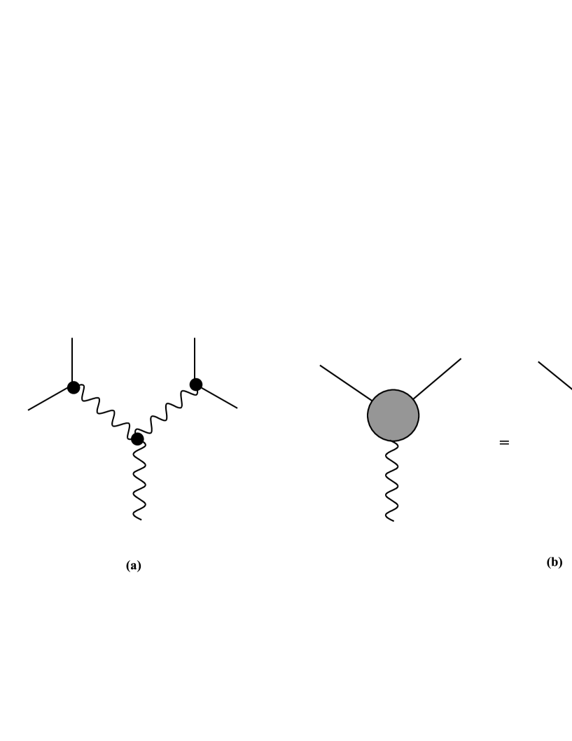
Figure 1: Diagrams contributing to the first post-Newtonian correction. (a) The tree diagram occurring because of the nonlinearity of the Einstein equations. (b) The one-loop form factor. Wavy lines represent gravitons, solid lines scalar particles.

This fact suggests the following interpretation of the correspondence principle when applied to the case of gravity: the effective gravitational field produced by a macroscopic body of mass $M$ consisting of $N$ particles turns into corresponding classical solution of the Einstein equations in the limit $M\to\infty,$ $N\to\infty.$

It is clear from the above discussion that the use of the effective action is essential for this interpretation: the quantum potential, being of the form

$$\Phi^{q}(r)=-N\frac{G(M/N)}{r}+{\rm const}_{1}N\frac{G^{2}(M/N)^{2}}{c^{2}r^{2}}+{\rm const}_{2}N\frac{G^{3}(M/N)^{3}}{c^{4}r^{3}}+\cdot\cdot\cdot,$$

for a macroscopic ($N$-particle) body of mass $M,$ would fail to reproduce classical potential other than Newtonian, since

$$\Phi^{q}(r)\to-\frac{GM}{r}~{}~{}{\rm when}~{}~{}N\to\infty.$$

Thus, the loop corrections of the order $\hbar^{0}$ are now considered on a equal footing with the tree corrections, and thereby are endowed direct physical meaning as describing deviations of the space-time metric from classical solutions of the Einstein equations in the case of finite $N.$

Like any other argument trying to assign physical meaning to the effective action, the above interpretation immediately runs up against the problem of its gauge dependence. In spite of being independent of the Planck constant, the $\hbar^{0}$ terms originating from the loop diagrams are not gauge-independent a priori. However, as will be demonstrated below, there is a strong evidence for that they are gauge-independent nevertheless. Namely, the $\hbar^{0}$ terms of the gravitational form factors of the scalar particle, contributing to the first post-Newtonian correction to the metric, turn out to be gauge-independent.

4 Generating functionals and Slavnov identities

As in Ref. [1], we consider the system of quantized gravitational and scalar matter fields. Dynamics of the scalar field denoted by $\phi,$ is described by the action

$$S_{\phi}=\frac{1}{2}{\displaystyle\int}d^{4}x\sqrt{-g}(g^{\mu\nu}\partial_{\mu}\phi\partial_{\nu}\phi-m^{2}\phi^{2}),$$ (6)

while the action for the gravitational field

$$S=-\frac{1}{k^{2}}{\displaystyle\int}d^{4}x\sqrt{-g}R,$$ (7)

$k$ being the gravitational constant.

The action $S+S_{\phi}$ is invariant under the following gauge transformations

$$\delta h_{\mu\nu}=\xi^{\alpha}\partial_{\alpha}h_{\mu\nu}+(\eta_{\mu\alpha}+h_{\mu\alpha})\partial_{\nu}\xi^{\alpha}+(\eta_{\nu\alpha}+h_{\nu\alpha})\partial_{\mu}\xi^{\alpha}\equiv D_{\mu\nu}^{\alpha}(h)\xi_{\alpha},$$

$$~{}~{}\delta\phi=\xi^{\alpha}\partial_{\alpha}\phi\equiv\tilde{D}^{\alpha}(\phi)\xi_{\alpha},$$ (8)

where $\xi^{\alpha}$ are the (infinitesimal) gauge functions. The generators $D,\tilde{D}$ span the closed algebra

$$D_{\mu\nu}^{\alpha,\sigma\lambda}D_{\sigma\lambda}^{\beta}-D_{\mu\nu}^{\beta,\sigma\lambda}D_{\sigma\lambda}^{\alpha}=f_{~{}~{}~{}\gamma}^{\alpha\beta}D_{\mu\nu}^{\gamma},$$

$$\tilde{D}^{\alpha}_{1}\tilde{D}^{\beta}-\tilde{D}^{\beta}_{1}\tilde{D}^{\alpha}=f^{\alpha\beta}_{~{}~{}~{}\gamma}\tilde{D}^{\gamma},$$ (9)

the ”structure constants” $f^{\alpha\beta}_{~{}~{}~{}\gamma}$ being defined by

$$f_{~{}~{}~{}\gamma}^{\alpha\beta}\xi_{\alpha}\eta_{\beta}=\xi_{\alpha}\partial^{\alpha}\eta_{\gamma}-\eta_{\alpha}\partial^{\alpha}\xi_{\gamma}.$$ (10)

Let the gauge invariance be fixed by the term

$$S_{gf}=\frac{1}{2\xi}\eta^{\alpha\beta}F_{\alpha}F_{\beta},$$

$$~{}~{}F_{\alpha}=\partial^{\mu}h_{\mu\alpha}-\frac{1}{2}\partial_{\alpha}h,~{}~{}h\equiv\eta^{\mu\nu}h_{\mu\nu}.$$ (11)

Next, introducing the Faddeev-Popov ghost fields $C_{\alpha},\bar{C}^{\alpha}$ we write the Faddeev-Popov quantum action [7]

$$S_{FP}=S+S_{\phi}+S_{gf}+\bar{C}^{\beta}F_{\beta}^{,\mu\nu}D_{\mu\nu}^{\alpha}C_{\alpha}.$$ (12)

$S_{FP}$ is still invariant under the following BRST transformations [8]

$$\delta h_{\mu\nu}=D_{\mu\nu}^{\alpha}(h)C_{\alpha}\lambda,$$

$$\delta\phi=\tilde{D}^{\alpha}(\phi)C_{\alpha}\lambda,$$

$$\delta C_{\gamma}=-\frac{1}{2}f^{\alpha\beta}_{~{}~{}~{}\gamma}C_{\alpha}C_{\beta}\lambda,$$

$$\delta\bar{C}^{\alpha}=\frac{1}{\xi}F^{\alpha}\lambda,$$ (13)

$\lambda$ being a constant anticommuting parameter.

The generating functional of Green functions

$$Z[T,J,\bar{\beta},\beta,K,\tilde{K},L]$$

$$={\displaystyle\int}dhd\phi dCd\bar{C}\exp\{i(\Sigma+\bar{\beta}^{\alpha}C_{\alpha}+\bar{C}^{\alpha}\beta_{\alpha}+T^{\mu\nu}h_{\mu\nu}+J\phi)\},$$ (14)

where

$$\Sigma=S_{FP}+K^{\mu\nu}D_{\mu\nu}^{\alpha}C_{\alpha}+\tilde{K}\tilde{D}^{\alpha}C_{\alpha}+L^{\gamma}\frac{1}{2}f^{\alpha\beta}_{~{}~{}~{}\gamma}C_{\alpha}C_{\beta},$$

the sets {$T^{\mu\nu},$ $J,$ $\bar{\beta}^{\alpha},$ $\beta_{\alpha}$} and {$K^{\mu\nu},$ $\tilde{K}$, $L^{\alpha}$} being the sources for the fields and BRST transformations, respectively [9].

To determine the dependence of field-theoretical quantities on the gauge parameter $\xi$, we modify the quantum action adding the term

$$YF_{\alpha}\bar{C}^{\alpha},$$

$Y$ being a constant anticommuting parameter [10]. Thus we write the generating functional of Green functions as

$$Z[T,J,\bar{\beta},\beta,K,\tilde{K},L,Y]={\displaystyle\int}dhd\phi dCd\bar{C}\exp\{i(\Sigma$$

$$+YF_{\alpha}\bar{C}^{\alpha}+\bar{\beta}^{\alpha}C_{\alpha}+\bar{C}^{\alpha}\beta_{\alpha}+T^{\mu\nu}h_{\mu\nu}+J\phi)\}.$$ (15)

Finally, we introduce the generating functional of connected Green functions

$$W[T,J,\bar{\beta},\beta,K,\tilde{K},L,Y]=-i\ln Z[T,J,\bar{\beta},\beta,K,\tilde{K},L,Y],$$ (16)

and then define the effective action $\Gamma$ in the usual way as the Legendre transform of $W$ with respect to the mean fields

$$h_{\mu\nu}=\frac{\delta W}{\delta T^{\mu\nu}},~{}~{}\phi=\frac{\delta W}{\delta J},~{}~{}C_{\alpha}=\frac{\delta W}{\delta\bar{\beta}^{\alpha}},~{}~{}\bar{C}^{\alpha}=-\frac{\delta W}{\delta\beta_{\alpha}},$$ (17)

(denoted by the same symbols as the corresponding field operators):

$$\Gamma[h,\phi,C,\bar{C},K,\tilde{K},L,Y]$$

$$=W[T,J,\bar{\beta},\beta,K,\tilde{K},L,Y]-\bar{\beta}^{\alpha}C_{\alpha}-\bar{C}^{\alpha}\beta_{\alpha}-T^{\mu\nu}h_{\mu\nu}-J\phi.$$ (18)

Evaluation of derivatives of diagrams with respect to the gauge parameters is a more easy task than their direct calculation in arbitrary gauge. This is because these derivatives can be expressed through another set of diagrams with more simple structure. The rules for such a transformation of diagrams are conveniently summarized in the Slavnov identities corresponding to the generating functional (4). Since these identities are widely used in what follows, their derivation will be briefly described below [10].

First of all, we perform a BRST shift (4) of integration variables in the path integral (4). Equating the variation to zero we obtain the following identity

$${\displaystyle\int}dhd\phi dCd\bar{C}\left[iY\bar{C}^{\alpha}F_{\alpha}^{,\mu\nu}D^{\beta}_{\mu\nu}C_{\beta}+i\frac{Y}{\xi}F_{\alpha}^{2}+T^{\mu\nu}\frac{\delta}{\delta K^{\mu\nu}}+J\frac{\delta}{\delta\tilde{K}}-\bar{\beta}^{\alpha}\frac{\delta}{\delta L^{\alpha}}-i\beta_{\alpha}\frac{F^{\alpha}}{\xi}\right]$$

$$\exp\{i(\Sigma+YF_{\alpha}\bar{C}^{\alpha}+\bar{\beta}^{\alpha}C_{\alpha}+\bar{C}^{\alpha}\beta_{\alpha}+T^{\mu\nu}h_{\mu\nu}+J\phi)\}=0.$$ (19)

Next, the second term in the square brackets in Eq. (4) can be transformed with the help of the quantum ghost equation of motion, obtained by performing a shift $\bar{C}\to\bar{C}+\delta\bar{C}$ of integration variables in the functional integral (4):

$${\displaystyle\int}dhd\phi dCd\bar{C}\left[F_{\gamma}^{,\mu\nu}D_{\mu\nu}^{\alpha}C_{\alpha}-YF_{\gamma}+\beta_{\gamma}\right]\exp\{\cdot\cdot\cdot\}=0,$$

from which it follows that

$$Y{\displaystyle\int}dhd\phi dCd\bar{C}\left[i\bar{C}^{\gamma}F_{\gamma}^{,\mu\nu}D_{\mu\nu}^{\alpha}C_{\alpha}+\beta_{\gamma}\frac{\delta}{\delta\beta_{\gamma}}\right]\exp\{\cdot\cdot\cdot\}=0,$$

where we used the property $Y^{2}=0$, and omitted the expression $\delta\beta_{\gamma}/\delta\beta_{\gamma}\sim\delta(0)$. Putting this all together, we rewrite Eq. (4)

$$\left(T^{\mu\nu}\frac{\delta}{\delta K^{\mu\nu}}+J\frac{\delta}{\delta\tilde{K}}-\bar{\beta}^{\alpha}\frac{\delta}{\delta L^{\alpha}}-\frac{1}{\xi}\beta_{\alpha}F^{\alpha,\mu\nu}\frac{\delta}{\delta T^{\mu\nu}}-Y\beta_{\gamma}\frac{\delta}{\delta\beta_{\gamma}}-2Y\xi\frac{\partial}{\partial\xi}\right)Z=0.$$ (20)

This is the Slavnov identity for the generating functional of Green functions we are looking for. In terms of the generating functional of connected Green functions, it looks like

$$T^{\mu\nu}\frac{\delta W}{\delta K^{\mu\nu}}+J\frac{\delta W}{\delta\tilde{K}}-\bar{\beta}^{\alpha}\frac{\delta W}{\delta L^{\alpha}}-\frac{1}{\xi}\beta_{\alpha}F^{\alpha,\mu\nu}\frac{\delta W}{\delta T^{\mu\nu}}-Y\beta_{\gamma}\frac{\delta W}{\delta\beta_{\gamma}}-2Y\xi\frac{\partial W}{\partial\xi}=0.$$ (21)

It can be transformed further into an identity for the generating functional of proper vertices: with the help of equations

$$T^{\mu\nu}=-\frac{\delta\Gamma}{\delta h_{\mu\nu}},~{}~{}J=-\frac{\delta\Gamma}{\delta\phi},~{}~{}\bar{\beta}^{\alpha}=\frac{\delta\Gamma}{\delta C_{\alpha}},~{}~{}\beta_{\alpha}=-\frac{\delta\Gamma}{\delta\bar{C}^{\alpha}},$$

which are the inverse of Eqs. (17), and the relations

$$\frac{\delta W}{\delta K^{\mu\nu}}=\frac{\delta\Gamma}{\delta K^{\mu\nu}},~{}~{}\frac{\delta W}{\delta\xi}=\frac{\delta\Gamma}{\delta\xi},{\rm~{}~{}etc.}$$

we rewrite Eq. (21)

$$\frac{\delta\Gamma}{\delta h_{\mu\nu}}\frac{\delta\Gamma}{\delta K^{\mu\nu}}+\frac{\delta\Gamma}{\delta\phi}\frac{\delta\Gamma}{\delta\tilde{K}}+\frac{\delta\Gamma}{\delta C_{\alpha}}\frac{\delta\Gamma}{\delta L^{\alpha}}-\frac{F^{\alpha}}{\xi}\frac{\delta\Gamma}{\delta\bar{C}^{\alpha}}+Y\frac{\delta\Gamma}{\delta\bar{C}^{\alpha}}\bar{C}^{\alpha}+2Y\xi\frac{\partial\Gamma}{\partial\xi}=0.$$ (22)

Written down via the reduced functional

$${\Gamma_{0}}=\Gamma-\frac{1}{2\xi}F_{\alpha}F^{\alpha}-YF_{\sigma}\bar{C}^{\sigma},$$ (23)

the latter equation takes particularly simple form

$$\frac{\delta\Gamma_{0}}{\delta h_{\mu\nu}}\frac{\delta\Gamma_{0}}{\delta K^{\mu\nu}}+\frac{\delta\Gamma_{0}}{\delta\phi}\frac{\delta\Gamma_{0}}{\delta\tilde{K}}+\frac{\delta\Gamma_{0}}{\delta C_{\sigma}}\frac{\delta\Gamma_{0}}{\delta L^{\sigma}}+2Y\xi\frac{\partial\Gamma_{0}}{\partial\xi}=0.$$ (24)

5 The $\hbar^{0}$ radiative corrections to the gravitational form factors

Let us now turn to the explicit evaluation of the radiative corrections. In this section, $\xi$-independence of the loop amendment to the first post-Newtonian classical correction given by the second term in Eq. (5) will be proved. The only loop diagram we need to consider is the one pictured in Fig. 1(b). Other one-loop diagrams do not contain terms proportional to the $\sqrt{-p^{2}},$ responsible for the $1/r^{2}$ behavior of the form factors, while higher-loop diagrams are of higher orders in the Newton constant $G.$

To evaluate the $\xi$-derivative of diagram 1(b), we use the Slavnov identity (24). Extracting terms proportional to the source $Y,$ we get

$$2\xi\frac{\partial\Gamma_{1}}{\partial\xi}=\frac{\delta\Gamma_{1}}{\delta h_{\mu\nu}}\frac{\delta\Gamma_{2}}{\delta K^{\mu\nu}}+\frac{\delta\Gamma_{1}}{\delta\phi}\frac{\delta\Gamma_{2}}{\delta\tilde{K}},$$ (25)

where $\Gamma_{1,2}$ are defined by

$$\Gamma_{1}=\Gamma_{0}|_{Y=0},~{}~{}\Gamma_{2}=\frac{\partial\Gamma_{0}}{\partial Y}.$$

At the one-loop level, Eq. (25) is just

$$2\xi\frac{\partial\Gamma^{(1)}_{1}}{\partial\xi}=\frac{\delta\Gamma^{(0)}_{1}}{\delta h_{\mu\nu}}\frac{\delta\Gamma^{(1)}_{2}}{\delta K^{\mu\nu}},$$ (26)

since the external scalar lines are on the mass shell

$$\frac{\delta S_{\phi}}{\delta\phi}=0.$$

Diagrams with two scalar and one graviton external lines, giving rise to the root singularity in the right hand side of Eq. (26), are represented in Fig. 2.

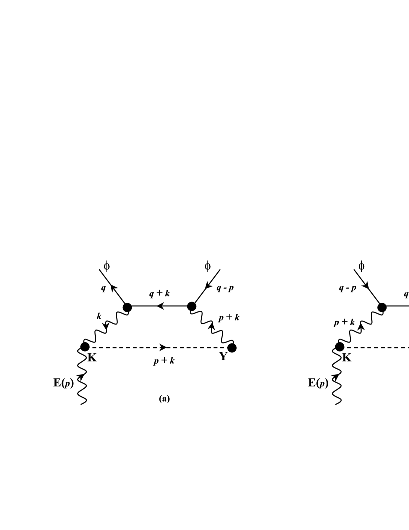
Figure 2: Diagrams with two scalar and one graviton external lines, containing the terms proportional to the square root of $(-p^{2})$ in the right hand side of Eq. (26). Dashed lines represent ghosts.

The corresponding analytical expressions

$$I_{3(a)}(p,q)=-iE^{\mu\nu}(p)~{}\mu^{\varepsilon}{\displaystyle\int}\frac{d^{4-\varepsilon}k}{(2\pi)^{4}}\left\{\frac{1}{2}W^{\alpha\beta\gamma\delta}q_{\gamma}(k_{\delta}+q_{\delta})-m^{2}\frac{\eta^{\alpha\beta}}{2}\right\}G_{\phi}$$

$$\times\left\{\frac{1}{2}W^{\rho\tau\sigma\lambda}(q_{\sigma}-p_{\sigma})(k_{\lambda}+q_{\lambda})-m^{2}\frac{\eta^{\rho\tau}}{2}\right\}\xi D^{(0)\eta}_{\rho\tau}\tilde{G}_{\eta}^{\xi}(k+p),$$

$$\times\tilde{G}_{\xi}^{\zeta}(p+k)\left\{k_{\zeta}\delta_{\mu\nu}^{\chi\theta}-\delta_{\zeta\mu}^{\chi\theta}(k_{\nu}+p_{\nu})-\delta_{\zeta\nu}^{\chi\theta}(k_{\mu}+p_{\mu})\right\}G_{\chi\theta\alpha\beta}(k),$$ (27)

$$I_{3(b)}(p,q)=I_{3(a)}(p,p-q),$$

where the following notation is introduced:

$$W^{\alpha\beta\gamma\delta}=\eta^{\alpha\beta}\eta^{\gamma\delta}-\eta^{\alpha\gamma}\eta^{\beta\delta}-\eta^{\alpha\delta}\eta^{\beta\gamma},~{}~{}\delta_{\alpha\beta}^{\mu\nu}=\delta_{\alpha}^{\mu}\delta_{\beta}^{\nu}+\delta_{\alpha}^{\nu}\delta_{\beta}^{\mu},$$

$G_{\mu\nu\sigma\lambda}$ is the graviton propagator defined by

$$\frac{\delta^{2}S}{\delta h_{\rho\tau}\delta h_{\mu\nu}}G_{\mu\nu\sigma\lambda}=-\delta_{\sigma\lambda}^{\rho\tau},$$

$$G_{\mu\nu\sigma\lambda}=-\frac{W_{\mu\nu\sigma\lambda}}{\Box}+(\xi-1)(\eta_{\mu\sigma}\partial_{\nu}\partial_{\lambda}+\eta_{\mu\lambda}\partial_{\nu}\partial_{\sigma}+\eta_{\nu\sigma}\partial_{\mu}\partial_{\lambda}+\eta_{\nu\lambda}\partial_{\mu}\partial_{\sigma})\frac{1}{\Box^{2}},$$ (28)

$\tilde{G}^{\alpha}_{\beta}$ is the ghost propagator

$$\tilde{G}^{\alpha}_{\beta}=-\frac{\delta^{\alpha}_{\beta}}{\Box},$$

satisfying

$$F_{\alpha}^{,\mu\nu}D^{(0)\beta}_{\mu\nu}\tilde{G}^{\gamma}_{\beta}=-\delta_{\alpha}^{\gamma},~{}~{}D^{(0)\alpha}_{\mu\nu}\equiv D^{\alpha}_{\mu\nu}(h=0),$$

$G_{\phi}$ is the scalar particle propagator

$$G_{\phi}=\frac{1}{\Box+m^{2}},$$

$E^{\mu\nu}$ stands for the linearized Einstein tensor

$$E^{\mu\nu}=R^{\mu\nu}-\frac{1}{2}\eta^{\mu\nu}R_{\alpha\beta}\eta^{\alpha\beta},~{}~{}R_{\mu\nu}=\frac{1}{2}(\partial^{\alpha}\partial_{\mu}h_{\alpha\nu}+\partial^{\alpha}\partial_{\nu}h_{\alpha\mu}-\Box h_{\mu\nu}-\partial_{\mu}\partial_{\nu}h),$$

$\mu$ – arbitrary mass scale, and $\varepsilon=4-d,$ $d$ being the dimensionality of space-time. To simplify the tensor structure of diagram Fig. 2(a), the use has been made of the identity

$$\frac{1}{\xi}F^{\alpha,\mu\nu}G_{\mu\nu\sigma\lambda}(x)=-D^{(0)\beta}_{\sigma\lambda}\tilde{G}_{\beta}^{\alpha}(x),$$

which is nothing but the well-known first Slavnov identity at the tree level; it is easily obtained differentiating Eq. (21) twice with respect to $\beta_{\alpha}$ and $T^{\mu\nu}$, and setting all the sources equal to zero.

The tensor multiplication in Eq. (5) is conveniently performed with the help of the new tensor package for the REDUCE system [12]

$$I_{3(a)}(p,q)=-iE^{\mu\nu}(p)~{}\mu^{\varepsilon}{\displaystyle\int}\frac{d^{4-\varepsilon}k}{(2\pi)^{4}}\frac{1}{k^{4}}\frac{1}{(k+p)^{4}}\frac{1}{m^{2}-(k+q)^{2}}$$

$$\times\xi[\eta_{\mu\nu}k^{2}m^{2}\{(kp)-(kq)\}\{k^{2}+2(kq)\}+k_{\mu}k_{\nu}k^{4}\xi(p^{2}-2m^{2})$$

$$+2k_{\mu}k_{\nu}k^{2}(kq)(2\xi-1)(p^{2}-2m^{2})+4k_{\mu}(k_{\nu}+p_{\nu})(kq)^{2}(\xi-1)(p^{2}-2m^{2})$$

$$+k_{\mu}p_{\nu}k^{4}(-2\xi m^{2}+\xi p^{2}-2m^{2})+2k_{\mu}p_{\nu}k^{2}(kq)(-4\xi m^{2}+2\xi p^{2}-p^{2})$$

$$+2k_{\mu}q_{\nu}k^{4}(p^{2}-m^{2})+4k_{\mu}q_{\nu}k^{2}(kq)(p^{2}-m^{2})-2p_{\mu}p_{\nu}k^{2}m^{2}\{k^{2}+2(kq)\}$$

$$+2p_{\mu}q_{\nu}k^{2}\xi\{(kp)-(kq)\}\{k^{2}+4(kq)\}+4p_{\mu}q_{\nu}k^{2}(kq)\{p^{2}-m^{2}+(kq)-(kp)\}$$

$$+8p_{\mu}q_{\nu}(kq)^{2}(\xi-1)\{(kp)-(kq)\}+2p_{\mu}q_{\nu}k^{4}(p^{2}-m^{2})$$

$$+2q_{\mu}q_{\nu}k^{4}\{(kq)-(kp)\}+4q_{\mu}q_{\nu}k^{2}(kq)\{(kq)-(kp)\}].$$ (29)

Evaluation of the loop integrals can be automatized to a considerable extent if the Schwinger parametrization of denominators in Eq. (5) is used

$$\frac{1}{k^{4}}=\int_{0}^{\infty}dy~{}y\exp\{yk^{2}\},~{}~{}\frac{1}{(k+p)^{4}}=\int_{0}^{\infty}dx~{}x\exp\{x(k+p)^{2}\},$$

$$\frac{1}{k^{2}+2(kq)}=-\int_{0}^{\infty}dz\exp\{z[k^{2}+2(kq)]\}.$$ (30)

It is convenient to apply these formulae as they stand, i.e., eluding cancellation of the $k^{2}$ factors in Eq. (5). The $k$-integrals are then evaluated using

$$\int~{}d^{d}k\exp\{k^{2}(x+y+z)+2k^{\mu}(xp_{\mu}+zq_{\mu})\}$$

$$=i\left(\frac{\pi}{x+y+z}\right)^{\frac{d}{2}}\exp\left\{\frac{p^{2}xy-m^{2}z^{2}}{x+y+z}\right\},$$

$$\int~{}d^{d}k~{}k_{\alpha}\exp\{k^{2}(x+y+z)+2k^{\mu}(xp_{\mu}+zq_{\mu})\}=$$

$$=i\left(\frac{\pi}{x+y+z}\right)^{\frac{d}{2}}\exp\left\{\frac{p^{2}xy-m^{2}z^{2}}{x+y+z}\right\}\left[-\frac{xp_{\alpha}+zq_{\alpha}}{x+y+z}\right],$$

etc. up to six $k$-factors in the integrand.

From now on, all formulae will be written out for the sum

$$I\equiv I_{3(a)}(p,q)+I_{3(b)}(p,q).$$

Changing the integration variables $(x,y,z)$ to $(t,u,v)$ via

$$x=\frac{t(1+t+u)v^{2}}{m^{2}(1+\alpha tu)},~{}~{}y=\frac{u(1+t+u)v^{2}}{m^{2}(1+\alpha tu)},~{}~{}z=\frac{(1+t+u)v^{2}}{m^{2}(1+\alpha tu)},~{}~{}\alpha\equiv-\frac{p^{2}}{m^{2}},$$

integrating $v$ out, subtracting the ultraviolet divergence

$$I^{{\rm div}}=\frac{1}{32\pi^{2}\varepsilon}\left(\frac{\mu}{m}\right)^{\varepsilon}E^{\mu\nu}(p)\eta_{\mu\nu}\xi^{2}(p^{2}-2m^{2}),$$

setting $\varepsilon=0$, and retaining only the leading at $p^{2}\to 0$ terms, we obtain

$$(I-I^{{\rm div}})_{{\varepsilon}\to 0}$$

$$=\frac{E^{\mu\nu}(p)\xi}{16\pi^{2}}\int_{0}^{\infty}\int_{0}^{\infty}dudt\left\{\frac{8m^{2}(\xi-1)}{p^{2}DN^{3}}\left(q_{\mu}q_{\nu}-\frac{m^{2}}{p^{2}}p_{\mu}p_{\nu}\right)\left(6-\frac{9}{D}+\frac{4}{D^{2}}\right)\right.$$

$$\left.+\frac{\eta_{\mu\nu}m^{2}}{DN}\left(1+\frac{12\xi m^{2}}{N^{2}p^{2}}-\frac{8\xi m^{2}}{DN^{2}p^{2}}-\frac{5}{D}+\frac{4}{D^{2}}\right)\right\},$$

$$D\equiv 1+\alpha ut,~{}~{}N\equiv 1+u+t.$$ (31)

Now, using Eqs. (6) of the Appendix, it is straightforward to show that the remaining $(u,t)$-integral is zero:

$$(I-I^{{\rm div}})_{{\varepsilon}\to 0}=0.$$

The first and the second lines in Eq. (5) cancel independently of each other, and so do the terms with and without $\xi$-factor in the second line.

Thus, the $\xi$-independence of the one-loop $\hbar^{0}$ contribution to the form factor Fig. 2(b) is proved. As was explained in Sec. 3, this fact allows us to consider this contribution as describing deviations of the space-time metric from classical solutions of the Einstein equations in the case when the gravitational field is produced by only one particle of mass $m$. Now we can use the results of the work [1] to determine the actual value of these deviations. Restoring the ordinary units, with the help of Eqs. (55),(65) of Ref. [1], and Eq. (28) we obtain

$$h^{{\rm loop}}_{\mu\nu}(p)=-\frac{\pi^{2}G^{2}}{c^{2}\sqrt{-p^{2}}}\left(3m^{2}\eta_{\mu\nu}+q_{\mu}q_{\nu}+7m^{2}\frac{p_{\mu}p_{\nu}}{p^{2}}\right).$$ (32)

In particular, for the static field of a massive particle at rest, the quantum correction to the time component of the metric, in the coordinate space,

$$h^{{\rm loop}}_{00}(r)=-\frac{2G^{2}m^{2}}{c^{2}r^{2}}.$$

Together with Eq. (2), this finally gives the following expression for the first post-Newtonian correction to the gravitational potential of a body with mass $M,$ consisting of $N$ identical (scalar) particles with mass $m=M/N$

$$\Phi(r)=-\frac{GM}{r}+\frac{G^{2}M^{2}}{2c^{2}r^{2}}-\frac{G^{2}M^{2}}{Nc^{2}r^{2}}.$$ (33)

It remains only to make the following important remark. As was already noted in Sec. 2, any attempt to give a self-contained notion of gravitational (or any other) field has to start, despite its ultimate purpose, with examination of matter interactions. Having restricted to zeroth order in the Planck constant $\hbar,$ however, we made the explicit introduction of additional matter playing the role of a measuring device superfluous. Indeed, whatever kind of matter is considered, its quantum corrected equations of motion to the order $\hbar^{0}$ are obtained simply substituting the value (33) in place of the potential entering the ordinary classical equations. Any other quantum corrections due to nonlinearity of interaction of the measuring apparatus with the gravitational field will be of higher orders in the Planck constant. In other words, the value of the effective gravitational field detected in the course of observation of the apparatus motion will be just (33). This is why interpretation given in Sec. 3 was formulated in terms of the effective equations of motion of the gravitational, rather than matter, field.

6 Discussion and Conclusions

The gauge-independence of the gravitational form factors, underlying our interpretation of the $\hbar^{0}$ loop contribution, is proved only for a particular, though most important practically, choice of gauge. Furthermore, the case of many-loop diagrams giving rise to the higher post-Newtonian corrections has not been touched upon at all. On the other hand, it is hardly believed that the gauge dependence cancellation found out in Sec. 5 is accidental. It takes place for any $\xi$ as well as for every independent tensor structure of diagram Fig. 1(b).

A very specific feature of this cancellation must be emphasized: it holds only for the $\hbar^{0}$ part of the form factors. For instance, the logarithmical part of $I$ (which is of the order $\hbar^{1}$) is not zero. This raises the question of reasons the gauge dependence cancellation originates from. The point is that the Slavnov identities, being valid only for the totals of diagrams, cannot provide such reason, although they do allow one to simplify calculation of the gauge-dependent parts of diagrams.

As was shown in Sec. 3, the use of the effective action is essential in establishing the correct correspondence between the classical and quantum theories of gravity. This makes the problem of physical interpretation of the effective action beyond the $\hbar^{0}$ order even more persistent. It was mentioned in Sec. 2 that such interpretation can probably be given via the introduction of point-particles into the theory. It should be noted, however, that this approach cannot be justified from the first principles of quantum theory, and therefore is out of our present concern. Nevertheless, one may hope that the phenomenological approach advanced in Ref. [3] can be developed in a consistent manner, e.g., along the lines of Refs. [4, 5].

Finally, let us consider possible astrophysical applications of our results. As we saw in Sec. 3, the loop contributions to the post-Newtonian corrections are normally highly suppressed: their relative value for the stars is of the order $10^{-56}-10^{-58}.$ Things are different, however, if an object consisting of strongly interacting particles is considered. In this case, additivity of individual contributions, implied in the course of derivation of Eq. (33), does not take place. In the limit of infinitely-strong interaction, the object is to be considered as a particle, i.e., one has to set $N=1$ in Eq. (33). The post-Newtonian corrections are then essentially different from those given by the classical General Relativity.

An example of objects of this type is probably supplied by the black holes. It should be noted, however, that the very existence of the horizon is now under question. The potential $\Phi(r)$ may well turn out to be a regular function of $r$ when all the $\hbar^{0}$ loop corrections are taken into account.

Appendix

The integrals

$$J_{nm}\equiv\int_{0}^{\infty}\int_{0}^{\infty}\frac{dudt}{(A+t+u)^{n}(B+\alpha tu)^{m}},$$

encountered in Sec. 5, can be evaluated as follows. Consider the auxiliary quantity

$$J(A,B)=\int_{0}^{\infty}\int_{0}^{\infty}\frac{dudt}{(A+t+u)(B+\alpha tu)},$$

where $A,B>0$ are some numbers eventually set equal to 1. Performing an elementary integration over $u,$ we get

$$J(A,B)=\int_{0}^{\infty}dt~{}\frac{\ln B-\ln\{\alpha t(A+t)\}}{B-\alpha t(A+t)}.$$

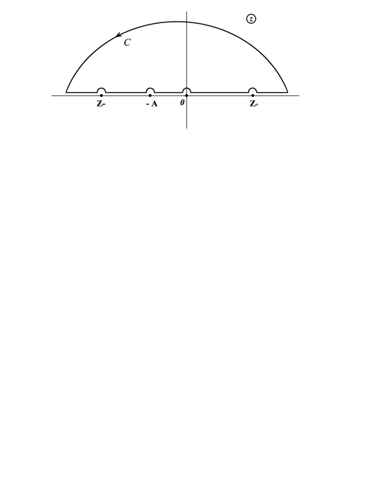
Figure 3: Contour of integration in Eq. (34)

Now consider the integral

$$\tilde{J}(A,B)=\int_{C}dzf(z,A,B),~{}~{}f(z,A,B)=\frac{\ln B-\ln\{\alpha z(A+z)\}}{B-\alpha z(A+z)},$$ (34)

taken over the contour $C$ shown in Fig. 3. $\tilde{J}(A,B)$ is zero identically. On the other hand,

$$\tilde{J}(A,B)$$

$$=\int^{-A}_{-\infty}dw~{}\frac{\ln B-\ln\{\alpha w(A+w)\}}{B-\alpha w(A+w)}+\int_{-A}^{0}dw~{}\frac{\ln B-\ln\{-\alpha w(A+w)\}+i\pi}{B-\alpha w(A+w)}$$

$$+\int_{0}^{+\infty}dw~{}\frac{\ln B-\ln\{\alpha w(A+w)\}+2i\pi}{B-\alpha w(A+w)}-i\pi\sum\limits_{z_{+},z_{-}}{\rm Res}f(z,A,B),$$

$z_{\pm}$ denoting the poles of the function $f(z,A,B),$

$$z_{\pm}=-\frac{A}{2}\pm\sqrt{\frac{B}{\alpha}+\frac{A^{2}}{4}}.$$

Change $w\to-A-w$ in the first integral. A simple calculation then gives

$$J(A,B)=\frac{\pi^{2}}{2\sqrt{\alpha}}B^{-1/2}\left(1+\frac{\alpha A^{2}}{4B}\right)^{-1/2}-\frac{1}{2}\int_{0}^{A}dt~{}\frac{\ln B-\ln\{\alpha t(A-t)\}}{B+\alpha t(A-t)}.$$ (35)

The roots are contained entirely in the first term on the right of Eq. (35). The integrals $J_{nm}$ are found by repeated differentiation of Eq. (35) with respect to $A,B$. Expanding $(1+\alpha A^{2}/4B)^{-1/2}$ in powers of $\alpha,$ we find the leading terms needed in Sec. 5

$$J^{{\rm root}}_{11}=\frac{\pi^{2}}{2\sqrt{\alpha}},~{}~{}J^{{\rm root}}_{12}=\frac{\pi^{2}}{4\sqrt{\alpha}},~{}~{}J^{{\rm root}}_{13}=\frac{3\pi^{2}}{16\sqrt{\alpha}},$$

$$J^{{\rm root}}_{31}=-\frac{\pi^{2}}{16}\sqrt{\alpha},~{}~{}J^{{\rm root}}_{32}=-\frac{3\pi^{2}}{32}\sqrt{\alpha},~{}~{}J^{{\rm root}}_{33}=-\frac{15\pi^{2}}{128}\sqrt{\alpha}.$$ (36)

References

- [1] J. F. Donoghue, Phys. Rev. Lett. 72, 2996 (1994); Phys. Rev. D50, 3874 (1994); Perturbative Dynamics of Quantum General Relativity, invited plenary talk at the ”Eighth Marcel Grossmann Conference on General Relativity”, Jerusalem (1997).
- [2] B. S. DeWitt, Phys. Rev. 162, 1195 (1967).
- [3] D. Dalvit and F. Mazzitelli, Phys. Rev. D56, 7779 (1997); Quantum Corrections to the Geodesic Equation, talk presented at the meeting ”Trends in Theoretical Physics II”, Buenos Aires, Argentina (1998).
- [4] K. A. Kazakov and P. I. Pronin, Phys. Rev. D62, 044043 (2000).
- [5] K. A. Kazakov and P. I. Pronin, Nucl. Phys. B 573, 536 (2000).
- [6] R. Kallosh and I. V. Tyutin, Yad. Fiz., 17, 190 (1973) [Sov. J. Nucl. Phys. 17, 98 (1973)].
- [7] L. D. Faddeev and V. N. Popov, Phys. Lett. 25B, 29 (1967).
- [8] C. Becchi, A. Rouet, and R. Stora, Ann. of Phys. 98, 287 (1976); Commun. Math. Phys. 42, 127 (1975); I. V. Tyutin, Report FIAN 39 (1975).
- [9] J. Zinn-Justin, in Trends in Elementary Particle Physics, edited by H. Rollnik and K. Dietz, Springer-Verlag, Berlin (1975), p. 2.
- [10] N. K. Nielsen, Nucl. Phys. B101, 173 (1975); H. Kluberg-Stern and J. B. Zuber, Phys. Rev. D 12, 467, 3159 (1975).
- [11] R. E. Kallosh, O. V. Tarasov, and I. V. Tyutin, Nucl. Phys. B137, 145 (1978).
- [12] P. I. Pronin and K. V. Stepanyantz, in New Computing Technick in Physics Research. IV., edited by B. Denby and D. Perred-Gallix, World Scientific, Singapure (1995), p. 187.