3D Gravity, Point Particles
and
Liouville Theory

Abstract

This paper elaborates on the bulk/boundary relation between negative cosmological constant 3D gravity and Liouville field theory (LFT). We develop an interpretation of LFT non-normalizable states in terms of particles moving in the bulk. This interpretation is suggested by the fact that “heavy” vertex operators of LFT create conical singularities and thus should correspond to point particles moving inside AdS. We confirm this expectation by comparing the (semi-classical approximation to the) LFT two-point function with the (appropriately regularized) gravity action evaluated on the corresponding metric.

I Introduction

The fact that Liouville theory describes asymptotic degrees of freedom of negative cosmological constant 3D gravity has been recognized some time ago [1]. Since then the appearance of LFT as an effective theory at asymptotic infinity was re-confirmed by many authors, see [2, 3] and a more recent reference [4]. However, all these results demonstrate only a relation between the classical theories: classical gravity in the bulk and classical LFT on the boundary. What concerns us in this paper is the relation between the corresponding quantum theories. Indeed, there is a growing evidence, see [5], that Liouville theory does make sense quantum mechanically. It is then interesting to ask: exactly how much of quantum gravity in the bulk, if any, is described by quantum LFT on the boundary? This question is of interest for 3D quantum gravity, for if this theory makes sense by itself, without embedding into string theory, the quantum LFT is a candidate for its holographic description. This question is also of interest in the context of string theory, for LFT is a part of the sigma model that is believed to be dual to the string theory on AdS${}_{3}\times S^{3}\times T^{4}$. Thus, by studying quantum LFT one might be able to learn something new about string theory on AdS₃, a subject of recent interest.

In this paper we make a step towards 3D quantum gravity interpretation of quantum LFT. We consider LFT vertex operators. These are local, or, in the terminology of [6], microscopical operators, which create states that are non-normalizable because of the change in the topology these operators introduce. Depending on its conformal dimension, such an operator creates either a conical singularity or a puncture at the point where it acts. In this paper we show that vertex operators on the boundary should be interpreted as describing point particles in the bulk. To see this, consider a point particle moving inside Euclidean AdS. It creates a line of conical singularities, which pierces the boundary at two points, and endows the boundary metric with angle deficits at those points. This is precisely the same boundary configuration as the one created by two vertex operators. We are thus led to interpreting one of these operators as creating a particle, and the other as annihilating it after its evolution in the bulk. The angle deficit created depends on the conformal dimension of the operator. As we shall see, the CFT relation between mass and conformal dimension translates then into the usual in gravity relation between mass and the angle deficit. To give more evidence in support of this interpretation we compare the bulk and boundary partition functions. More precisely, we consider the semi-classical approximation, in which the bulk and boundary partition functions are dominated by the corresponding classical solutions, and show that the (appropriately regulated) bulk action evaluated on Euclidean AdS with a line of conical singularities is equal to the Liouville theory action evaluated on the Liouville field that describes a metric with two conical singularities.

Thus, vertex operators of LFT on the boundary receive the 3D interpretation of operators creating point particles inside AdS. This interpretation is potentially interesting for 3D quantum gravity, for one can use the results available from LFT to analyze processes involving point particles, such as, e.g., the black hole creation process of [8]. On the other hand, this interpretation gives a new perspective on LFT itself, for it means that the non-normalizable states of LFT that are created by vertex operators are physically interesting states of the theory and should receive more attention.

At this point it seems appropriate to mention that the idea to consider quantum LFT as a theory of quantum gravity in 3D was a subject of criticism, in particular by [7]. The reason for this criticism is as follows. Although by tuning the coupling constant the central charge of Liouville theory can be made to be equal to Brown-Henneaux central charge [9], it is known that if one only considers the normalizable states in LFT, because of the mass gap, the effective central charge is rendered to be one. Since it is the effective central charge that appears in the formula for the asymptotic density of states, the number of states in the quantum LFT is then not enough to account for the BTZ black hole entropy, see [10] for a good discussion of this issue. Then it seems unavoidable [7] that one needs the whole of string theory to account for the microscopic origin of the black hole entropy, and that LFT only describes macroscopic, thermodynamical degrees of freedom of gravity. However, in view of the interpretation of the non-normalizable states of LFT as physical states corresponding to the point particles inside AdS, one may have to reconsider the issue with the density of states. Indeed, if one allows the non-normalizable states, then there is no mass gap in the spectrum, which might mean that one has to consider the full central charge in the formula for the density of states. While this remains to be shown, it is certainly true that the point particle states are there to be considered as the states contributing to the black hole entropy, and this might change the state counting. This might invalidate the point of [7]. We, however, do not attempt to settle this issue in the present paper. Let us note that non-normalizable modes were considered as relevant to the black hole entropy problem in [11].

Thus, in this paper we take –as a working hypothesis– the viewpoint that quantum LFT provides one with a holographic description of quantum gravity, or some sector of it. Although the possibility of such a relation between the two quantum theories has been discussed, a precise identification between LFT and gravity, namely a relation between the cosmological constant and the coupling constant of Liouville theory, does not seem to have appeared in the literature. The correspondence we propose is as follows. The 3D Einstein-Hilbert action is:

$$S_{gr}={1\over 16\pi G}\int_{\cal M}d^{3}x\sqrt{g}(R-2\Lambda),$$ (1)

where $G$ is Newton constant, the integral is taken over the 3D manifold $\cal M$ that we consider gravity on, $\Lambda$ is the cosmological constant, which we assume to be negative, $g$ is the determinant of the metric, which we consider to be of Euclidean signature, $R$ is the trace of Ricci. The Liouville theory action is:

$$A_{L}[\phi]=\int d^{2}x\left[{1\over 4\pi}(\partial_{a}\phi)^{2}+\mu e^{2b\phi}\right].$$ (2)

Here $\phi$ is the Liouville field, $b$ is the coupling constant of the theory and $\mu$ is a constant of the dimension of $1/({\rm length})^{2}$, which sets a scale for the theory. We leave the region over which the integral is taken unspecified for now. All physical quantities in LFT depend not on $b$, but on the quantity

$$Q=b+{1\over b}.$$ (3)

The identification we propose is:

$$Q^{2}={l\over 4G\hbar}={l\over 4l_{p}},$$ (4)

where $l=1/\sqrt{-\Lambda}$ is the curvature radius of AdS. The regime when the semi-classical approximation in LFT is valid (small $b$) corresponds, according to (4) to large curvature radii, and, thus, is also the regime when the semi-classical approximation in gravity should be valid. In this regime, the Liouville central charge:

$$c_{L}=1+6Q^{2}$$ (5)

matches the Brown-Henneaux central charge [9] $3l/2G\hbar$. Interestingly, the so-called strong coupling region in LFT, $1<c_{L}<25$, of which very little is known, corresponds in view of (4), to the Planckian regime $l<16l_{p}$ on the gravity side. Another interesting fact is that, unlike in AdS₅/CFT₄ correspondence, where there is only one limit on the CFT side that corresponds to the semi-classical limit on the gravity side, there are two different limits one can reach this regime in our example. Because of the famous Liouville theory duality $b\to 1/b$, both small and large coupling regimes in LFT correspond to the semi-classical regime on the gravity side.

The paper is organized as follows. Section II reviews some basic facts about quantum LFT. Section III gives the point particle interpretation of LFT vertex operators. We conclude with a discussion of the results obtained.

We should emphasize that, although the relation between 3D gravity and Liouville theory can be discussed for the Lorentzian signature as well, this paper treats only the Euclidean case. To interpret the Euclidean results we obtain in terms of the real world Lorentzian signature gravity one has to adopt a version of the analytic continuation procedure. Although this question is important, it is not considered in this paper.

II Preliminaries: quantum Liouville theory

In this section we review some well-known facts about Liouville theory. Our main source is [12], which the reader is referred to for more details. Our conventions and notations on LFT are the same as in this reference.

Liouville theory is described by the action (2). Usually one also adds to the Lagrangian a term proportional to $\phi R$, where $R$ is the curvature scalar of a fixed background metric, and adjusts the coefficient in front of this term so that the action is independent of the background. For our purposes, however, it is more convenient to work in the flat background (this is also the choice of [12]). Then the integral of $\phi R$ translates into a bunch of boundary terms, see below. Although by appropriately choosing the boundary terms one can define LFT on any Riemann surface, see [13], for the purposes of this paper it is sufficient to consider the case of a sphere. The LFT on a sphere corresponds to field $\phi$ defined on the whole complex plane with the following asymptotics for $|z|\to\infty$:

$$\phi(z,\bar{z})=-Q\ln(z\bar{z})+O(1),$$ (6)

where $Q$ is given by (3). To make the action (2) well-defined on such fields, one introduces a large disc $\Omega$ of radius $R\to\infty$ and adds a boundary term to the action:

$$A_{L}=\int_{\Omega}d^{2}x\left[{1\over 4\pi}(\partial_{a}\phi)^{2}+\mu e^{2b\phi}\right]+{Q\over\pi R}\int_{\partial\Omega}dl\,\phi+2Q^{2}\ln{R}.$$ (7)

The last term is needed to make the action finite as $R\to\infty$.

The vertex operators of LFT are:

$$V_{\alpha}(x)=e^{2\alpha\phi(x)},$$ (8)

where $x$ is a point on $S^{2}$. They are primary operators of conformal dimension:

$$\Delta_{\alpha}=\alpha(Q-\alpha).$$ (9)

Correlation functions of vertex operators are formally defined as the following functional integral:

$${\cal G}_{\alpha_{1},\ldots,\alpha_{n}}(x_{1},\ldots,x_{n})=\int{\cal D}\phi\,V_{\alpha_{1}}(x_{1})\cdots V_{\alpha_{n}}(x_{n})e^{-A_{L}[\phi]}.$$ (10)

The integral must be taken over the fields satisfying the boundary condition (6).

The scale dependence of correlators is:

$${\cal G}_{\alpha_{1},\ldots,\alpha_{n}}(x_{1},\ldots,x_{n})=(\pi\mu)^{(Q-\sum\alpha_{i})/b}F_{\alpha_{1},\ldots,\alpha_{n}}(x_{1},\ldots,x_{n}),$$ (11)

where $F_{\alpha_{1},\ldots,\alpha_{n}}(x_{1},\ldots,x_{n})$ is independent of the scale $\mu$. Instead of correlation functions at fixed scale $\mu$ we shall often consider the fixed area correlation functions ${\cal G}^{(A)}_{\alpha_{1},\ldots,\alpha_{n}}(x_{1},\ldots,x_{n})$, given by the functional integral over fields with

$$A=\int dx^{2}\,e^{2b\phi}$$ (12)

fixed. The fixed area correlators are related to (10) by

$${\cal G}_{\alpha_{1},\ldots,\alpha_{n}}(x_{1},\ldots,x_{n})=\int_{0}^{\infty}{\cal G}^{(A)}_{\alpha_{1},\ldots,\alpha_{n}}(x_{1},\ldots,x_{n})e^{-\mu A}{dA\over A}\,,$$ (13)

so that

$${\cal G}^{(A)}_{\alpha_{1},\ldots,\alpha_{n}}(x_{1},\ldots,x_{n})=\left({A\over\pi}\right)^{(\sum\alpha_{i}-Q)/b}{F_{\alpha_{1},\ldots,\alpha_{n}}(x_{1},\ldots,x_{n})\over\Gamma((Q-\sum\alpha_{i})/b)}\,.$$ (14)

The spectrum of LFT consists of the states created by $V_{\alpha}$ with

$$\alpha={Q\over 2}+iP.$$ (15)

These are the normalizable states. One can also consider the “states” created by $V_{\alpha}$ with $0<\alpha<Q/2$. These operators create conical singularities and thus correspond to non-normalizable states.

Classical LFT, which is that with the interaction term being $e^{\phi}$, appears as the semi-classical limit of the theory described by the action (2). The semi-classical limit of LFT corresponds to $b\to 0$. One then introduces a new field:

$$\varphi=2b\phi,$$ (16)

which becomes the classical Liouville field in this limit. The “quantum” action (2) is then:

$$A_{L}[\phi]={1\over b^{2}}S_{Liouv}[\varphi],$$ (17)

where

$$S_{Liouv}[\varphi]={1\over 8\pi}\int d^{2}x\left[{1\over 2}(\partial_{a}\varphi)^{2}+8\pi\mu b^{2}e^{\varphi}\right]$$ (18)

is the classical Liouville action. There are also some boundary terms to be added to this action, see below. Varying the classical action with respect to $\varphi$ one finds that locally $\varphi$ satisfies the classical Liouville equation:

$$\Delta\varphi=8\pi\mu b^{2}e^{\varphi}.$$ (19)

Then the metric $ds^{2}=e^{\varphi}|dz|^{2}$ is a metric of constant negative curvature $-8\pi\mu b^{2}$. The importance of the classical Liouville action lies in the fact that correlation functions of vertex operators are, in the semi-classical limit, dominated by $S_{Liouv}$ evaluated on the corresponding solution to the Liouville equation. Let us consider as an example the case of “heavy” vertex operators, which is relevant for this paper. Let us take $\alpha_{i}=\eta_{i}/b$ with $\eta_{i}$ of order $O(1)$, and consider the case $\sum\eta_{i}<1$ so that there is no solution to (19) with negative curvature. The relevant solution is that with positive curvature. One has to impose the area constraint

$$A=\int dx^{2}\,e^{\varphi}$$ (20)

and consider the positive curvature Liouville equation

$$\Delta\varphi=-{8\pi\over A}\left(1-\sum\eta_{i}\right)e^{\varphi}$$ (21)

with the field $\varphi$ satisfying the following boundary conditions:

$$\varphi(z,\bar{z})=-2\ln{|z|^{2}}+O(1)\qquad{\rm at}\quad|z|\to\infty$$ (22)

$$\varphi(z,\bar{z})=-2\eta_{i}\ln{|z-x_{i}|^{2}}+O(1)\qquad{\rm at}\quad z\to x_{i}.$$ (23)

The fixed area correlation functions are then dominated by the fixed area Liouville action:

$${\cal G}^{(A)}_{\alpha_{1},\ldots,\alpha_{n}}(x_{1},\ldots,x_{n})\sim\exp{\left(-{1\over b^{2}}S_{Liouv}^{(A)}\right)}.$$ (24)

Here the fixed area Liouville action $S_{Liouv}^{(A)}$ is the one without the interaction term, and contains boundary terms around singularities at $x_{i}$:

$$S_{Liouv}^{(A)}[\varphi]={1\over 8\pi}\int_{\Omega}dx^{2}\left[{1\over 2}(\partial_{a}\varphi)^{2}\right]+\phi_{\infty}+2\ln{R}-\sum_{i}\left(\eta_{i}\varphi_{i}+2\eta_{i}^{2}\ln{\epsilon_{i}}\right).$$ (25)

Here $\Omega$ is a disc of radius $R$ with small discs of radii $\epsilon_{i}$ cut out around each of the singularities at $x_{i}$, and

$$\varphi_{i}={1\over 2\pi\epsilon_{i}}\int_{\partial\Omega_{i}}dl\,\varphi.$$ (26)

As an example, let us give the fixed area action for the case of two vertex operators, each of $\alpha=\eta/b$. For simplicity, we insert the operators at $z=0,\infty$. The classical Liouville field in this case is:

$$e^{\varphi}={A\over\pi(1-2\eta)}{a^{2}(z\bar{z})^{a-1}\over(1+(z\bar{z})^{a})^{2}},$$ (27)

where $a=1-2\eta$. In the next section we shall see how this field is obtained. One can then evaluate the fixed area action (25) on this field. The resulting fixed area action for two vertex operators is:

$$S_{Liouv}^{(A)}=(1-2\eta)\left(\ln{A\over\pi}+\ln(1-2\eta)-1\right).$$ (28)

In the next section we compare this action, or, more precisely, a related quantity, to the free energy of AdS metric with a line of conical singularity.

III Particle interpretation

We would now like to describe a point particle interpretation of the LFT vertex operators $V_{\alpha}$ with $0<\alpha<Q/2$. Let us, as before, when analyzing the semi-classical approximation of LFT, introduce a parameter $\eta:\alpha=\eta/b$. This parameter measures the angle deficits of the metric described by the classical Liouville field. To see this, we must rewrite the vertex operator $V_{\alpha}$ as:

$$V_{\alpha}=e^{2b\phi\,\eta/b^{2}}=e^{\varphi\eta/b^{2}}.$$ (29)

When $b\to 0$, the correlation functions are dominated by the extremum of the classical Liouville action (18) with sources $\sum_{i}\eta\varphi(x_{i})$. This then introduces $\delta$-function type singularities on the right hand side of (19):

$$\Delta\varphi=8\pi\mu b^{2}e^{\varphi}-\sum_{i}\eta_{i}\delta_{x_{i}}.$$ (30)

Recalling that $\Delta\varphi=-\sqrt{g}R$, where $g$ is the determinant of the metric $ds^{2}=e^{\varphi}|dz|^{2}$ and $R$ is its curvature, we see that the angle deficits at $x_{i}$ are equal to $4\pi\eta_{i}$.

Let us recall now that the analysis [9] of asymptotic symmetries of $\Lambda<0$ 3D gravity gives the following relation between mass and conformal dimension:

$$Ml=\Delta+\bar{\Delta}.$$ (31)

It is exactly this relation between $M$ and $\Delta$ (plus an analogous relation for the angular momentum) that needs to be inserted into the Cardy formula for the CFT asymptotic density of states to get the correct Bekenstein-Hawking entropy for BTZ black hole, see [14]. For vertex operators under consideration the conformal dimension is real, which means that particles they are to describe are non-rotating. Let us consider the case of “not very heavy” vertex operators: $\eta\ll 1$. Then $\Delta_{\alpha}\approx Q\alpha\approx\eta/b^{2}$. Recalling the relation (4) between $l$ and $Q$, we see that, in this regime, the mass is given by $M=\eta/2G$. This means that the angle deficit is $8\pi GM$, which is correct gravity relation between mass and the angle deficit. We thus see that it holds for our vertex operators, provided the parameter $\eta$ is small. This is the first check of the particle interpretation of vertex operators.

FIG. 1.: The AdS space with a line of conical singularities can be described as AdS with a wedge removed.

To perform a more serious check we need to compare the partition functions on the bulk and boundary sides. Although the two-point function on the LFT side is known for any value of the coupling, see [15, 12], there is no quantum gravity calculation of the point particle partition function. The best we can do is to compare the partition functions in the regime $l\gg l_{p}$ when one can use the semi-classical approximation in the bulk. This is the regime $b\ll 1$ on the LFT side, and, thus, one also uses the semi-classical approximation here. The semi-classical approximation to the fixed area two-point function in LFT is given by $\exp{-S_{Liouv}^{(A)}/b^{2}}$ with the fixed area action given above by (28). We have to compare this quantity to the $\exp{-S_{gr}}$ evaluated on the AdS metric with a line of conical singularities. The metric describing a point particle moving in a constant curvature space was first obtained in [16].

Let us describe this geometry in a language that can be easily generalized to more complicated situations, e.g., with more than one particle. The metric is obtained as a discrete identification of the AdS space with respect to a discrete subgroup $\Sigma$ of the isometry group, which in our case is ${\rm SL}(2,{\mathbb{C}})$. To obtain a single line of conical singularities inside AdS we have to take $\Sigma$ to be generated by a single elliptic element. Then the line of conical singularities is the line of fixed points of the transformation generated by this element. Action of an isometry inside AdS generates a conformal transformation on the boundary. Any such transformation has two fixed points (possibly coinciding), and in our case these are the points on the boundary where it is intersected by the particle worldline. The quotient of the boundary with respect to $\Sigma$ is, in general, a Riemann surface, and, in our case, a sphere with two conical singularities. Let us denote the boundary by ${\cal S}$, and the quotient ${\cal S}/\Sigma$ by $X$. Properties of the projection map $\pi_{\Sigma}\to X$ are very important. It is the knowledge of this map that allows one to find the corresponding Liouville field, which in our example is given by (27). Let us now see how this technology works.

It is most convenient for our purposes to use the upper half-space model of AdS. The hyperbolic metric in this model is:

$$ds^{2}={l^{2}\over\xi^{2}}\left(d\xi^{2}+|dw|^{2}\right),$$ (32)

where $\xi$ is the coordinate that runs orthogonally to the boundary ${\cal S}$ located at $\xi=0$, and $w$ is a homomorphic coordinate on ${\cal S}$. Note that ${\cal S}$ is the whole extended complex plane, for the point at infinity also belongs to it. In this model geodesics are half-circles (or straight lines) orthogonal to the boundary. By a conformal transformation we can always put one of the conical singularities (=fixed points) at $w=0$ and the other at $w=\infty$. Then the particle’s worldline is a straight line orthogonal to the boundary. Let $\Sigma$ be generated by a rotation on an angle $2\pi a$ around this line. The angle deficit created is then $2\pi(1-a)=4\pi\eta$, see Fig. 1.

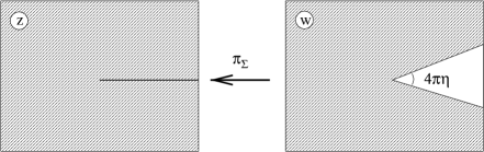
FIG. 2.: Complex planes $z$ and $w$. The map from $w$ to $z$ is a covering, which is branched at fixed points of elliptic generators, in our case at $0,\infty$.

The quotient $X$ of ${\cal S}$ by $\Sigma$ is again a complex plane, with two singular points. Let us introduce a homomorphic coordinate $z$ on $X$. The projection map $\pi_{\Sigma}:{\cal S}\to X$ is easy to determine:

$$\pi_{\Sigma}:w\to z=w^{{1\over a}}.$$ (33)

Note that it is finitely branched only for integer $a$. As we have said, the knowledge of this map allows one to determine the Liouville field. In our case we would like to have a Liouville field on the $z$-plane that describes a constant positive curvature metric of total area $A$. We get such a field from the sphere metric on the $w$-plane. This metric is given by:

$$ds^{2}={A\over\pi(1-2\eta)}{|dw|^{2}\over(1+w\bar{w})^{2}},$$ (34)

where we have divided $A$ by the factor $(1-2\eta)$ to correct for the fact that only a portion of the $w$-plane is mapped to the $z$-plane. Using the inverse of the map (33) it is easy to see that the Liouville field on the $z$-plane is indeed given by (27). Comparing the asymptotics of this field for $z\to 0$ with that given in (23) one finds that $(1-a)$ must indeed be identified with $2\eta$, and, thus, $4\pi\eta$ is the angle deficit. The simple analysis of this paragraph can be generalized to much more complex situations. It is true in general that the knowledge of the projection map $\pi_{\Sigma}$, or rather of its inverse, which is called the uniformization map, is equivalent to the knowledge of the corresponding Liouville field. A generalization of the construction described dates back to Poincare, who used it as an approach to the problem of uniformization of Riemann surfaces.

Having described the quotient geometry, let us evaluate the gravity action on the corresponding metric. In 3D Einstein-Hilbert action reduces on shell to the volume of the corresponding space:

$$S_{gr}=-{V\over 4\pi Gl^{2}}.$$ (35)

For spaces that are non-compact, as in our case, this volume diverges, and we need to employ some kind of regularization procedure. In asymptotically AdS spaces, where the volume grows as $Al/2$, where $A$ is the boundary area, one has a natural regularization by subtracting $Al/2$. Thus, the idea is to introduce a family of regularizing surfaces, labelled by a parameter $\epsilon$, which approach the boundary as $\epsilon\to 0$. One should then calculate the volume $V_{\epsilon}$ above a surface of fixed $\epsilon$, subtract $A_{\epsilon}l/2$, and take the limit $\epsilon\to 0$. As we shall see, the area subtraction does not kill all of the divergence: there is still a logarithmic divergence to be taken care of. However, as it was discussed, e.g., in [17], this divergence does have a CFT interpretation, namely that of a scale dependence of the partition functions due to the conformal anomaly.

Let us first see how this procedure works on the simplest case of AdS space itself. The modification to incorporate the deficit angle is then straightforward. Let us first do the calculation in the unit ball model, where we don’t have to deal with subtleties coming from the point at infinity. The AdS metric in the unit ball model, in spherical coordinates is:

$$ds^{2}={4l^{2}\over(1-r^{2})^{2}}(dr^{2}+r^{2}\sin^{2}\theta d\phi^{2}+r^{2}d\theta^{2}).$$ (36)

The volume inside a sphere of radius $r=R$ is:

$$V_{R}=4\pi l^{3}\left[{R(1+R^{2})\over(1-R^{2})^{2}}-{1\over 2}\ln{{1+R\over 1-R}}\right].$$ (37)

The area of this sphere is:

$$A_{R}=4\pi l^{2}{4R^{2}\over(1-R^{2})^{2}}.$$ (38)

The regularized gravity action is then:

$$S_{gr}=-{1\over 4\pi Gl^{2}}\left[V_{R}-{A_{R}l\over 2}\right]=-{l\over 4G}\left[{4R\over(1+R)^{2}}-2\ln{{1+R\over 1-R}}\right].$$ (39)

Introducing $\epsilon:R=1-\epsilon$, and using the relation (4) for $b\ll 1$, we get:

$$S_{gr}={1\over b^{2}}\left[-1+\ln{{A_{\epsilon}\over\pi l^{2}}}+O(\epsilon)\right].$$ (40)

The expression in square brackets, in the limit $\epsilon\to 0$, coincides with the fixed area Liouville action for the sphere, which can be obtained from (28) for $\eta=0$.

It is now straightforward to modify the result (40) to incorporate the angle deficit. First, when integrating over $\phi$ to get (37), (38), we have to integrate not over the whole $2\pi$ but over $2\pi(1-2\eta)$. This modifies (37), (38) by multiplying them by $(1-2\eta)$. Second, to get (40) from (39), we have to express $2\ln{(1+R)/(1-R)}$ in terms of $A_{\epsilon}$. This introduces another modification. We now have:

$$2\ln{{1+R\over 1-R}}=\ln{A_{\epsilon}\over\pi(1-2\eta)l^{2}}+O(\epsilon).$$ (41)

Thus, the final result for the regularized gravity action is:

$$S_{gr}={1\over b^{2}}(1-2\eta)\left[-1+\ln{{A_{\epsilon}\over\pi l^{2}}}-\ln{(1-2\eta)}+O(\epsilon)\right].$$ (42)

This is almost the same as (28), except for the sign in front of the last term in square brackets. This seeming discrepancy comes from the fact that we are comparing the gravity action (42) to the wrong Liouville action. Namely, there are two different Liouville actions to consider: one evaluated on the Liouville field on the $z$-plane, this action is given by (28), and another action calculated for the Liouville field on the $w$-plane. To go between the two planes one uses a conformal transformation, see Fig. 2. Thus, the two actions are not the same, and differ by the action evaluated on the Liouville field that describes this conformal transformation. It is not hard to show that this difference between the Liouville actions on the $z$ and $w$-planes is exactly $(1-2\eta)\ln{(1-2\eta)}$. Thus, the (regularized) gravity action evaluated on AdS metric with a line of conical singularities does agree with the semi-classical approximation to the LFT two-point function, when the later is computed as the Liouville action on the $w$-plane.

We would now like to present another way to perform the calculation that leads to (42). Instead of using the unit ball model, we shall now use the upper half-space picture. Although this other calculation may seem more awkward, one does have to use this type of calculation in more complicated situations, e.g., when the boundary is a Riemann surface, as was considered in [18], or when we have more than two punctures. We would like to present this other way of getting the same result, first, because it is easily generalizable to other situations, and, second, because one can clearly see how the Liouville theory (on the $w$-plane) appears.

Thus, let us work in the upper half-space. We need to choose a family of regularizing surfaces. A natural choice is:

$$\xi(w,\bar{w})=\epsilon e^{-\varphi(w,\bar{w})/2},$$ (43)

where $\varphi$ is the Liouville field corresponding to the sphere:

$$e^{\varphi(w,\bar{w})}={A\over\pi(1+w\bar{w})^{2}}.$$ (44)

Here

$$A=\int_{{\cal S}}dx^{2}e^{\varphi}.$$ (45)

For small $\epsilon$, and for sufficiently small $|w|$, surfaces (43) are just the spheres $r=1-\epsilon\sqrt{4\pi/A}$ of the unit ball model. However, unlike the surfaces $r=const$, the surfaces (43) touch the boundary ${\cal S}$ at $w=\infty$. Because of this, the volume $V_{\epsilon}$ above a surface (43) diverges. Let us introduce an additional regularization by a half-sphere of a radius $R$, see Fig. 3.

FIG. 3.: Surfaces of the upper-half space calculation.

Let us now calculate the volume above a surface (43) and inside the half-sphere. It is given by:

$$l^{3}\int dx^{2}\left({1\over 2\xi_{min}^{2}}-{1\over 2\xi_{max}^{2}}\right).$$ (46)

Here $\xi_{min}^{2}(x)=\epsilon^{2}\exp{-\varphi(x)}$ is the $\xi$ coordinate squared of the $\epsilon$-surface, and $\xi_{max}^{2}(x)=R^{2}-|x|^{2}$ is that for the half-sphere. The integral is taken over the region $x:\xi_{min}(x)\leq\xi_{max}(x)$. The integral of the second term in (46) can be taken. Then (46) becomes:

$$l^{3}\int dx^{2}\,{1\over 2\epsilon^{2}}e^{\varphi}-l^{3}\left(\pi\ln{{R\over\epsilon}}+{1\over 4R}\int dl\,\varphi\right)+O(\epsilon),$$ (47)

where the last integral is taken along the circle $|x|=R$. We also need to know the area of the $\epsilon$-plane. It is given by:

$$l^{2}\int dx^{2}\left({1\over\epsilon^{2}}e^{\phi}+{1\over 8}(\partial_{a}\varphi)^{2}+O(\epsilon)\right),$$ (48)

with integral taken over the same region as in (46). We get the regularized action by combining the volume and area:

$$S_{R}={1\over b^{2}}\left({1\over 8\pi}\int dx^{2}\,(\partial_{a}\varphi)^{2}+\ln{{R\over\epsilon}}+{1\over 4\pi R}\int dl\,\varphi+O(\epsilon)\right).$$ (49)

Note that we have not yet used the expression (44) for $\varphi$. Note also that the expression in brackets is almost the constant area Liouville action (25) for the case of no vertex operators. The only difference is that to get (25) one has to take the last two terms in (49) twice. This happens because our surfaces (43) behave at infinity differently from $r=const$ surfaces of the unit ball model. Our surfaces are only “good” near the origin of the complex plane. To cure the situation one can either introduce a “charge” at infinity, or, as we shall do, integrate only over a finite region of the complex plane $|x|\leq R=1$ and then take the result twice. Thus, we do the calculation by dividing the AdS in two halfs and calculating the action for one of them. It is not hard to see that this gives the right result:

$$S_{gr}=2S_{R=1}={1\over b^{2}}\left(-1+\ln{{A\over\pi}}-\ln\epsilon^{2}+O(\epsilon)\right).$$ (50)

Here we have used the expression (44) for $\varphi$ and took the integral of the “kinetic” Liouville term. This is the same result as we obtained earlier in the unit ball model, one just has to replace $A_{\epsilon}/l^{2}$ in (40) by $A/\epsilon^{2}$ of (50). The above calculation makes it clear, see (49), how the Liouville action appears. Also, as we already mentioned, it is this calculation that can be generalized to more complicated situations, in fact, to the case of the boundary being any Riemann surface, see [18]. It is true in general that, regularizing the gravity action with the family of surfaces (43), where $\varphi$ is the relevant Liouville field, one obtains the classical fixed area Liouville action as the result. A similar derivation of the Liouville action was used in [19], although the authors used a different coordinate system.

One can now modify the result (50) to incorporate the angle deficit. This is done similarly to what we did to get from (40) to (42). Again, one finds that the regularized gravity action is given by (42). To compare it with (28) we have to recall that there is a rescaling (33) to go from $w$ to $z$ plane. Taking into account this rescaling, one finds that the gravity and LFT actions agree.

IV Discussion

Thus, the particle interpretation of LFT vertex operators passes two tests: (i) CFT relation (31) between mass and conformal dimension becomes for these vertex operators the usual gravity relation between mass and the angle deficit (for small deficit angles); (ii) partition functions agree, in the semi-classical approximation $b\ll 1,l\gg l_{p}$. As we mentioned in the text, this agreement of the partition functions holds in a much more general situation than that of a single point particle. There is a computation, along the lines of our upper half-space computation of the previous section, which works also for compact Riemann surfaces, see [18], and can be extended to the most general case of Riemann surfaces with conical singularities and punctures. It shows that the regularized gravity action calculated using the regularizing surfaces (43) is equal to $1/b^{2}$ times the fixed area Liouville action, that is the one without the $e^{\varphi}$ term, evaluated on the relevant Liouville field. Thus, at least at the semi-classical level, the partition functions for gravity and LFT coincide, provided the identification (4) is made.

This is still, however, a classical result, because to arrive to it we only had to compare the classical actions. It does not by itself imply that quantum LFT has something to do with quantum gravity in 3D. To establish a relation between quantum theories we would have to calculate some quantity in quantum gravity, not in the semi-classical approximation, and then compare this quantity to the one calculated on the CFT side. The lack of a quantum theory of negative cosmological constant 3D gravity prevents us from establishing such a relation. Note, however, that the situation here is not much worse than that with AdS/CFT dualities, for which most of the evidence so far comes from the semi-classical checks. In our case we cannot do better because we don’t have a good theory of $\Lambda<0$ 3D quantum gravity, in string theory this happens because it is hard to do the full fledged string theory in backgrounds containing AdS.

There is, however, another line of reasoning, based on works on quantum dilogarithm [20, 21], quantization of Teichmuller spaces [22, 23, 24] and [25, 26], and quantum Liouville [5, 27], which gives strong additional support to the identification of quantum LFT with quantum theory of gravity in 3D. In three dimensions one can construct a discrete, lattice-type model of quantum gravity. Such a model was so far formulated for $\Lambda=0,\Lambda>0$ Euclidean 3D gravity. In the case $\Lambda=0$ it is known as Ponzano-Regge model [28], the $\Lambda>0$ case is usually referred to as Turaev-Viro model [29]. These are state sum models, for one first chops the space into, e.g., tetrahedra, labels edges of these tetrahedra in a certain way, and then sums over labellings. As one can show, the state sum is triangulation independent, that is, it is invariant under changes of triangulation. It is also known to reproduce the correct partition functions for a variety of manifolds, where the correct means that the same partition function can be obtained by more conventional methods, e.g., using the Chern-Simons path integral. The key point for us is that the triangulation independence of the states sum, which is the feature that makes these models well-defined, can be traced back to the fact that each of these models is based on a certain category of group representations. This is the usual ${\rm SO}(3)$ for Ponzano-Regge model and the quantum group ${\rm SU}_{q}(2)$ for Turaev-Viro model, with $q$ being a root of unity. Thus, the fact that these models make sense can be traced back to the fact that the set of irreducible representations of the corresponding groups closes under the operation of taking the tensor product. Let us now return to Liouville theory. As the recent work [5] shows, LFT seems to be consistent as a CFT, that is, satisfies the properties of the conformal bootstrap, because the algebra of conformal blocks of LFT is based on the algebra of irreducible representations of a certain quantum group. As the results of [5] indicate, there is a certain series of continuous irreducible representations of ${\rm SL}_{q}(2,{\mathbb{R}})$, with deformation parameter $q=\exp{\pi ib^{2}}$, which is closed under taking tensor products [27]. This property then guarantees the consistency of the quantum LFT. What is important for our discussion is that one could built a discrete state sum model of 3D quantum gravity out of the same representations that are of key importance for LFT. This model is guaranteed to be consistent, in the sense that it is triangulation independent, because of the category properties satisfied by the set of representations in question. It does not, however, guaranteed to be finite. Indeed, unlike the sum over a discrete set of representations in, e.g., Turaev-Viro model, for this model one would have to take an integral over a continuous family of representations. Assuming that such integrals can be given sense, this model would be a good candidate for a quantum theory of 3D negative cosmological constant gravity. It would be very interesting to construct such a bulk model; partial results in this direction are contained in the works of Kashaev [20, 21] on knot invariants from the quantum dilogarithm. Because the consistency of both this model and LFT would be based on using the same series of representations, it is very likely that this model will be related to quantum LFT, the later giving a holographic description of the former. A similar discussion of the relation between state sum models and boundary Liouville theory can be found in [30].

Accepting a possibility of bulk/boundary relation between $\Lambda<0$ gravity and Liouville theory, there are many interesting gravity calculations that can be done using LFT on the boundary. For example, it would be interesting to analyze the black hole creation process of [8] in the boundary theory. Another thing that has to be done is to settle the issue with the density of states in the theory. This could possibly be done by a method analogous to the one used in [31] to check the prediction [32] for the spectrum of string theory in AdS₃. We hope to return to these questions in future publications.

Our last comment is about relation to string theory in AdS₃. Recall [32] that the string spectrum in this case consists of a continuous part, which describes long strings moving off to infinity, and a discrete part, which is the spectrum of fundamental strings inside AdS. It is interesting that the gravity/LFT relation under discussion seems to give a very similar picture. The spectrum of LFT consists of a continuous part (15), which describes the zero mode of the field moving with a constant momentum to infinity, and another part, corresponding to vertex operators with $0<\alpha\leq Q/2$. This other part of the spectrum is interpreted in the present paper as corresponding to point particles. Note that it becomes discrete if one allows only the rational angle deficits, a natural choice from the point of view of functions on the boundary, which then become finitely branched. This would then be very similar to what one finds for strings. The continuous part of the spectrum has the same interpretation in terms of two-dimensional surface –worldsheet in string theory and “boundary” in our case– moving off to infinity. However, the discrete part of the spectrum corresponds to fundamental strings inside AdS on the string side, while in our case it would correspond to point particles moving inside the space. Provided this similarity is not superficial, it might lead to a new and interesting relation between the two so different objects.

Acknowledgements. I am grateful to L. Freildel for an important discussion and to G. Horowitz for suggestions on the first version of the manuscript. This work was supported in part by NSF grant PHY95-07065.

REFERENCES

- [1] O. Coussaert, M. Henneaux and P. van Driel, The asymptotic dynamics of three-dimensional Einstein gravity with a negative cosmological constant, Class. Quant. Grav. 12 2961-2966 (1995).
- [2] K. Skenderis and S. Solodukhin, Quantum effective action from the AdS/CFT correspondence, Phys. Lett. B472 316-322 (2000).
- [3] K. Bautier, F. Englert, M. Rooman and P. Spindel, The Fefferman-Graham ambiguity and AdS black holes, Phys. Lett. B479 291-298 (2000).
- [4] M. Rooman and Ph. Spindel, Holonomies, anomalies and the Fefferman-Graham ambiguity in AdS3 gravity, hep-th/0008147.
- [5] B. Ponsot and J. Techner, Liouville bootstrap via harmonic analysis on a noncompact quantum group, hep-th/9911110.
- [6] N. Seiberg, Notes on quantum Liouville theory and quantum gravity, Prog. Theor. Phys. Suppl. 102 319-349 (1990).
- [7] E. Martinec, Conformal field theory, geometry and entropy, hep-th/9809021.
- [8] H-J. Matschull, Black hole creation in (2+1)-dimensions, Class. Quant. Grav. 16 1069-1095 (1999).
- [9] J. D. Brown and M. Henneaux, Central charges in the canonical realization of asymptotic symmetries: an example from three-dimensional gravity, Comm. Math. Phys. 104 207-226 (1986).
- [10] S. Carlip, What we don’t know about BTZ black hole entropy, Class. Quant. Grav. 15 3609-3625 (1998).
- [11] Y. S. Myung, Entropy problem in the AdS(3)/CFT correspondence, hep-th/9809172.
- [12] A. B. Zamolodchikov and Al. B. Zamolodchikov, Structure constants and conformal bootstrap in Liouville field theory, Nucl. Phys. B477 577-605 (1996).
- [13] L. Takhtajan and P. Zograf, On uniformization of Riemann surfaces and the Weyl-Peterson metric on Teichmuller and Schottky spaces, Math. USSR Sbornik 60 297-313 (1988).
- [14] A. Strominger, Black hole entropy from near horizon microstates, JHEP 9802 009 (1998).
- [15] H. Dorn and H. J. Otto, Two and three point functions in Liouville theory, Nucl. Phys. B429 375-388 (1994).
- [16] S. Deser and R. Jackiw, Three-dimensional cosmological gravity: dynamics of constant curvature, Annals Phys. 153 405-416 (1984).
- [17] M. Hennigson and K. Skenderis, The holographic Weyl anomaly, JHEP 9807 023 (1998).
- [18] K. Krasnov, Holography and Riemann surfaces, hep-th/0005106.
- [19] N. Seiberg and E. Witten, The D1/D5 system and singular CFT, JHEP 9904 017 (1999).
- [20] R. M. Kashaev, Quantum dilogarithm as a 6j-symbol, Mod. Phys. Lett. A9 3757-3768 (1994).
- [21] R. M. Kashaev, The hyperbolic volume of knots from quantum dilogarithm Lett. Math. Phys. 39 269-275 (1997).
- [22] R. M. Kashaev, Quantization of Teichmuller spaces and the quantum dilogarithm, q-alg/9705021.
- [23] R. M. Kashaev, Liouville central charge in quantum Teichmuller theory, hep-th/9811203.
- [24] R. M. Kashaev, On the spectrum of Dehn twists in quantum Teichmuller theory, math.QA/0008148.
- [25] V. V. Fock, Dual Teichmuller spaces, dg-ga/9702018.
- [26] L. Chekhov and V. V. Fock, Quantum Teichmuller space, Theor. Math. Phys. 120 1245-1259 (1999).
- [27] B. Ponsot and J. Techner, Clebsch-Gordan and Racah-Wigner coefficients for a continuous series of representations of , math.QA/0007097.
- [28] G. Ponzano and T. Regge, Semiclassical limits of Racach coefficients, In Spectroscopic and theoretical methods in physics, ed. F. Block, North-Holland Amsterdam, 1968.
- [29] N. Reshetikhin and V. G. Turaev, Invariants of three manifolds via link polynomials and quantum groups, Invent. Math. 103, 547-597 (1991).
- [30] M. O’Loughlin, Boundary actions in Ponzano-Regge discretization, quantum groups and AdS(3), gr-qc/0002092.
- [31] J. Maldacena, H. Ooguri and J. Sohn, Strings in AdS3 and WZW model. Part II: Euclidean black hole, hep-th/0005183.
- [32] J. Maldacena and H. Ooguri, Strings in AdS3 and WZW model. Part I: the spectrum, hep-th/0001053.