hep-th/0008241
UTPT-00-10
NSF-ITP-99-145
TASI Lectures
on
Black Holes in String Theory
Amanda W. Peet
Department of Physics,
University of Toronto,
60 St. George St.,
Toronto, ON, M5S 1A7,
Canada.
“Whaia te iti kahuraḵi;
Ki te tuohu koe, me he mauḵa teitei”
“Aspire to the highest pinnacles;
If you should bow, let it be to a lofty mountain”
In Maori culture111Maori are the indigenous peoples in Aotearoa
(New Zealand), and in others throughout the world, the mountain is
revered and respected for its mana, awesome presence and sheer
majesty. This proverbial saying, then, encapsulates all that my
grandfather has meant to me; he has been my lofty mountain. His
wisdom, knowledge and guidance encouraged me throughout my life in the
pursuit of excellence. I therefore dedicate this review to him.
Dedication crafted by Maurice Gray, Kaumatua, Te Runaḵa Ki Otautahi O Ḵai Tahu, and gifted to the author.
1 GR black holes, and thermodynamics
Black holes have long been objects of interest in theoretical physics, and more recently also in experimental astrophysics. Interestingly, study of them has led to new results in string theory. Here we will study black holes and their -brane cousins in the context of string theory, which is generally regarded as the best candidate for a unified quantum theory of all interactions including gravity. Other approaches to quantum gravity, such as “quantum geometry”, have been recently discussed in works such as [1]. Other relatively recent reviews of black hole entropy in string theory have appeared in [2, 3, 4].
Black holes may arise in string theory with many different conserved quantum numbers attached. We will begin our discussion by studying two basic black holes of General Relativity; they are special cases of the string theory black holes.
Note that the units we will use throughout are such that only ; we will not suppress powers of the string coupling , the string length , or the Newton constant .
1.1 Schwarzschild black holes
The Schwarzschild metric is a solution of the action
| (1.1) |
The field equations following from this action are the source-free () Einstein equations
| (1.2) |
In standard Schwarzschild coordinates, the metric takes the form
| (1.3) |
Astrophysical black holes formed via gravitational collapse have a lower mass limit of a few solar masses. However, we will be interested in all sizes of black holes, for theoretical reasons; we will not discuss any mechanisms by which ‘primordial’ black holes might have formed. When we move to discussion of charged black holes, we will also ignore the fact that any astrophysical charged black hole discharges on a very short timescale via Schwinger pair production. The reader unhappy with this should simply imagine that the charges we put on our black holes are not carried by light elementary quanta in nature such as electrons.
Not all massive objects are black holes. In order for a small object to qualify as a black hole, we need at a minimum that its Schwarzschild radius be larger than its Compton wavelength, . This implies that . So the electron, which is about times lighter than the Planck mass, does not qualify.
The event horizon of a stationary black hole geometry occurs where
| (1.4) |
For the Schwarzschild solution, the above condition is the same as the condition but in general, e.g. for the Kerr black hole, the two conditions do not coincide. Note also that for an evolving geometry the event horizon does not even have a local definition; it is a global concept. In the present static case, solving for the event horizon locus we find a sphere, and the radius is in Schwarzschild coordinates
| (1.5) |
Although metric components blow up at , the horizon is only a coordinate singularity, as we can see by computing curvature invariants. Note that the source-free Einstein equations imply that the Ricci scalar and so the Ricci tensor . For the Riemann tensor we get
| (1.6) |
Therefore, the curvature at the horizon of a big black hole is weak, and it blows up at , the physical singularity.
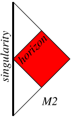
The Carter-Penrose diagram in Fig.1 shows the causal structure of the eternal Schwarzschild black hole spacetime. Note that, following tradition, only the plane is drawn, so that there is an implicit at each point. In gravitational collapse only part of this diagram is present, and it is matched onto a region of Minkowski space. In collapse situations there is of course no time reversal invariance, and so the Carter-Penrose diagram is not symmetric.

The Schwarzschild geometry is asymptotically flat, as can be seen by inspection of the metric at large-. Let us now inspect the geometry near the horizon. Define to be the proper distance, i.e. . Then
| (1.7) |
Near , . Now rescale time,
| (1.8) |
the metric becomes
| (1.9) |
From this form of the metric it is easy to see that if we Wick rotate , we will avoid a conical singularity if we identify the Euclidean time with period . Now, in field theory applications, we have the formal identification of the Euclidean Feynman path integral with a statistical mechanical partition function, and the periodicity in Euclidean time is identified as the inverse temperature. Tracing back to our original coordinate system, we identify the black hole temperature to be
| (1.10) |
This is the Hawking temperature of the black hole.
The use of Euclidean methods in quantum gravity has been discussed in, for example, [5]. There can be subtleties in doing a Wick rotation, however, which may mean that it is not a well-defined operation in quantum gravity in general. One thing which can go wrong is that there may not exist a Euclidean geometry corresponding to the original geometry with Lorentzian signature. In addition, smooth Euclidean spaces can turn into singular Lorentzian ones upon Wick rotation.
In any case, the result for the Hawking temperature as derived here can easily be replicated by other calculations, see e.g. the recent review of [6]. These results also tell us that the black hole radiates with a thermal spectrum, and that the Hawking temperature is the physical temperature felt by an observer at infinity.
Notice from (1.10) that increases as decreases, so that the specific heat is negative. This gives rise to runaway evaporation of the black hole at low mass. We can compute the approximate lifetime of the black hole from its luminosity, using the fact that it radiates (roughly) like a blackbody,
| (1.11) |
For astrophysical-sized black holes, this is much longer than the age of the Universe. For small black holes, however, there is a more pressing need to identify the endpoint of Hawking radiation. We will have more to say about this topic later when we discuss the Correspondence Principle. To find some numbers on what constitutes a ‘small’ vs. ‘large’ black hole in the context of evaporation, let us restore the factors of . We obtain an extra factor in the denominator of in the expression for . The result is that the mass of the black hole whose lifetime is the age of the universe, roughly 15 billion years, is kg. Such a black hole has a Schwarzschild radius of about a femtometre.
1.2 Reissner-Nordström black holes
For the case of Einstein gravity coupled to a gauge field, both the metric and gauge field can be turned on
| (1.12) |
There are two horizons, located at and .
Cosmic censorship requires that the singularity at be hidden behind a horizon, i.e.
| (1.13) |
The Hawking temperature is
| (1.14) |
Notice that the extremal black hole, with , i.e. , has zero temperature. It is a stable object, as it does not radiate. A phenomenon closely related to this and our previous result for Schwarzschild black holes is that the specific heat at constant charge is not monotonic. Specifically,
| (1.15) |
Consider the extremal geometry, and let the double horizon be at . Change the radial coordinate to
| (1.16) |
then
| (1.17) |
so that
| (1.18) |
We see that in these coordinates there is manifest symmetry; they are known as isotropic coordinates.
The extremal black hole geometry has an additional special property. Near the horizon ,
| (1.19) |
Defining yet another new coordinate
| (1.20) |
so that , we find a direct product of an anti-deSitter spacetime with a sphere:
Since the Reissner-Nordström spacetime is also asymptotically flat, we see that it interpolates between two maximally symmetric spacetimes [7]. In the units we use here, , which is a special relationship between the bosonic fields in the Lagrangian. It turns out that this means that the RN black hole possesses a supersymmetry, something about which we will have more to say in subsection (2.3).
1.3 Semiclassical gravity and black hole thermodynamics
Given some assumptions about the field content of the Lagrangian, classical no-hair theorems for black holes can be derived; see e.g. [8] for a modern treatment. For example, if there is a gauge field minimally coupled to Einstein gravity in , then the no-hair theorem states that an observer outside the black hole can measure only the mass , charge , and angular momentum of a black hole. These are the conserved quantum numbers associated to the long-range fields in the Lagrangian. The very limited amount of long-range hair means that, classically, we have a very limited knowledge of the black hole from the outside. Also, a black hole could have been formed via a wide variety of processes. This suggests that a black hole will possess a degeneracy of states, and hence an entropy, as a function of its conserved quantum numbers.
In the late 1960’s and early 1970’s, laws of classical black hole mechanics were discovered [9], which bear a striking resemblance to the laws of thermodynamics. The zeroth black hole law is that the surface gravity is constant over the horizon of a stationary black hole. The first law is
| (1.21) |
where is the angular velocity at the horizon and the electrostatic potential. The second law says that the horizon area must be nondecreasing in any (classical) process. Lastly, the third law says that it is impossible to achieve via a physical process such as emission of photons.
From (1.21) and other arguments, Bekenstein proposed [10] that the entropy of the black hole should be proportional to the area of the event horizon. Hawking’s semiclassical calculation of the black hole temperature
| (1.22) |
made the entropy-area identification precise by fixing the coefficient. (In the semiclassical approximation, the spacetime is treated classically, while matter fields interacting with it are treated quantum-mechanically.) In the reference frame of an asymptotically faraway observer, Hawking radiation is emitted at the horizon as a perfect blackbody. The thermal emission spectrum is then filtered by potential barriers encountered by the outgoing radiation, which arise from the varying gravitational potential, and give rise to “greybody factors”.
The Bekenstein-Hawking or Black Hole entropy is in any spacetime dimension
| (1.23) |
where is the area of the event horizon, and is the -dimensional Newton constant, which in units has dimensions of (length)d-2. This is a universal result for any black hole, applicable to any theory with Einstein gravity as its classical action. Note that the black hole entropy is a humongous number, e.g. for a four-dimensional Earth-mass black hole which has a Schwarzschild radius of order 1cm, the entropy is .
Up to constants, the black hole entropy is just the area of the horizon in Planck units. As it scales like the area rather than the volume, it violates our naive intuition about extensivity of thermodynamic entropy which we gain from working with quantum field theories. The area scaling has in fact been argued to be evidence for “holography”. There are several versions of holography, but the basic idea is that since the entropy scales like the area rather than the volume, the fundamental degrees of freedom describing the system are characterised by a quantum field theory with one fewer space dimensions and with Planck-scale UV cutoff. This idea was elevated to a principle by ’t Hooft and Susskind. The “AdS/CFT correspondence” does in fact provide an explicit and precise example of this idea. For more details, including references, see Susskind’s lectures on the Holographic Principle at this School [12].
As we will see later on in explicit examples, there are systems where the entropy of a zero-temperature black hole is nonzero. Note that this does not imply a violation of the third law of thermodynamics if the analogy between black hole mechanics and thermodynamics is indeed exact. There is no requirement in the fundamental laws of thermodynamics that the entropy should be zero at zero temperature; that version of the third law is a statement about equations of state for ordinary types of matter.
A subtlety which we have suppressed until now in discussing black hole thermodynamics is that an asymptotically flat black hole cannot really be in equilibrium with a heat bath. This is problematic if we wish to work in the canonical thermal ensemble. The trouble is the Jeans instability: even a low-density gas distributed throughout a flat spacetime will not be static but it will undergo gravitational collapse. Technical ways around this problem have been devised, such as putting the black hole in a box and keeping the walls of the box at finite temperature via the proverbial reservoir. This physical setup puts in an infrared cutoff which gets rid of the Jeans problem. It also alters the relation between the black hole energy and the temperature at the boundary (the walls of the box rather than infinity). This in turn results in a positive specific heat for the black hole. For a large box, which is appropriate if we wish to affect properties of the spacetime as little as possible, the black hole is always the entropically preferred state, but for a small enough box hot flat space results. For more details see [11].
As the black hole Hawking radiates, it loses mass, and its horizon area decreases, thereby providing an explicit quantum mechanical violation of the classical area-increase theorem. Since the area of the horizon is proportional to the black hole entropy, it might appear that this area decrease signals a violation of the second law. On the other hand, the entropy in the Hawking radiation increases, providing a possible way out. Defining a generalised entropy, which includes the entropy of the black hole plus the other stuff such as Hawking radiation,
| (1.24) |
was argued by Bekenstein to fix up the second law.
Using gedankenexperiments involving gravitational collapse and infalling matter, Bekenstein also argued that the entropy of a system of a particular volume is bounded above by the entropy of the black hole whose horizon bounds that volume. The Bekenstein bound is however not a completely general bound, as pointed out by Bekenstein himself. The system to which it applies must be one of “limited self-gravity”, and it must be a whole system not just a subsystem. Examples of systems not satisfying the bound include a closed FRW universe, or a super-horizon region in a flat FRW universe. In these situations, cosmological expansion drives the overall dynamics and self-gravity is not limited; the entropy in a big enough volume in such spacetimes will exceed the Bekenstein bound. Also, certain regions inside a black hole horizon violate the bound.
Bousso [13] has formulated a more general, covariant, entropy bound. A new ingredient in this construction is to use null hypersurfaces bounded by the area . The surfaces used are “light-sheets”, which are surfaces generated by light rays leaving which have nonpositive expansion everywhere on the sheet. The Bousso bound then says that the entropy on the sheets must satisfy
| (1.25) |
A proof of this bound was given in [14]; one or other of two conditions on the entropy flux across the light-sheets was required. These conditions are physically reasonable conditions for normal matter in semi-classical regimes below the Planck scale. The conditions can be violated, and so the bound does not follow from fundamental physical principles. It does however hold up in all semiclassical situations where light-sheets make sense, as long as the semiclassical approximation is used in a self-consistent fashion [13]. The generalised second law then works with the entropy defined as above. A recent discussion of semiclassical black hole thermodynamics [6] points out that there are no known gedankenexperiments which violate this generalised bound. See also a different discussion of holography in [15].
While the Bousso bound is a statement that makes sense only in a semiclassical regime, it may well be more fundamental, in that the consistent quantum theory of gravity obeys it.
1.4 The black hole information problem
Identifying the Bekenstein-Hawking entropy as the physical entropy of the black hole gives rise to an immediate puzzle, namely the nature of the microscopic quantum mechanical degrees of freedom giving rise to that thermodynamic entropy. Another puzzle, the famous information problem [16], arose from Hawking’s semiclassical calculation which showed that the outgoing radiation has a purely thermal character, and depends only on the conserved quantum numbers coupling to long-range fields. This entails a loss of information, since an infalling book and a vacuum cleaner of the same mass would give rise to the same Hawking radiation according to an observer outside the horizon. In addition, since the classical no-hair theorems allow observers at infinity to see only long-range hair, which is very limited, black holes are in the habit of gobbling up quantum numbers associated to all global symmetries.
In the context of string theory, which is a unified quantum theory of all interactions including gravity, information should not be lost. As a consequence, the information problem must be an artifact of the semiclassical approximation used to derive it. Information must somehow be returned in subtle correlations of the outgoing radiation. This point of view was espoused early on by workers including [22, 23] and collaborators following the original suggestion of Page [24]. Information return requires a quantum gravity theory with subtle nonlocality, a property which string theory appears to possess. The AdS/CFT correspondence is one context in which we have an explicit realization in principle of the information retention scenario, as discussed in Susskind’s lectures at this School. The information problem is therefore shifted to the problem of showing precisely how semiclassical arguments break down. This turns out to be a very difficult problem, and solving it is one of the foremost challenges in this area of string theory.
At the ITP Conference on Quantum Aspects of Black Holes in 1993, however, there were several scenarios on the market for solving the information problem. Nowadays, it is fair to say that the mainstream opinion in the string theory community has zeroed in on the information return scenario. Let us briefly mention some aspects of various scenarios to illustrate some useful physics points.
The idea that information is just lost in quantum gravity [16] has many consequences apt to make high energy theorists queasy, so we will not dwell on it. We just mention that one of them is that it usually violates energy conservation, although a refinement is possible [17] where clustering is violated instead. Another scenario is that all of the information about what fell into the black hole during its entire lifetime is stored in a remnant of Planckian size. The main problem with this scenario is that energy is needed in order to encode information, and a Planck scale remnant has very little energy. In addition, remnants as a class would need an enormous density of states in order to be able to keep track of all information that fell into any one of the black holes giving rise to the remnant. This enormous density of states of Planck scale objects is incompatible with any object known in string theory. Such a huge density of states could also lead to a phenomenological disaster if tiny virtual remnants circulate in quantum loops. Remnants also cause trouble in the thermal atmosphere of a big black hole [19]. A possibility for remnants is that they are baby universes. One approach to baby universes was to consider in a Euclidean approach our large universe and the effects on its physics due to a condensate of tiny (Planck-sized) wormholes. Arguments were made [20] that the tiny wormholes lead to no observable loss of quantum coherence in our universe. Nonetheless, the baby universe story does involve in-principle information loss in our universe, and the physics depends on selection of the wavefunction of the universe. It is also difficult [21] to be sure that there are only tiny wormholes present. Lastly, as we mentioned previously, Wick rotation from Euclidean to Lorentzian signature is not in general a well-understood operation in quantum gravity.
The original Hawking radiation calculation is semiclassical, i.e. the black hole is treated classically while the matter fields are treated quantum-mechanically. The computation of the thermal radiation spectrum, and subsequent computations, use at some point unwarranted assumptions about physics above the Planck scale. This is a fatal flaw in the argument for information loss. It has however been argued in [6] that the precise nature of this super-Planckian physics does not impact the Hawking spectrum very much, and that as such it is a robust semiclassical result. The information return devil is in the details, however. Susskind’s analogy between the black hole and a lump of coal fired on by a laser beam makes this quite explicit.
An interesting piece of semiclassical physics [25] is that all except a small part of the black hole spacetime near the singularity can be foliated by Cauchy surfaces called “nice slices”, which have the property that both infalling matter and outgoing Hawking radiation have low energy in the local frame of the slice. An adiabatic argument [25] then led to the conclusion that return of information in the framework of local field theory is difficult to reconcile with the existence of nice slices. One possibility is that the singularity plays an important role in returning information, although it can hardly do so in a local manner.
Showing that the information return scenario is inconsistent turns out to be very difficult. One of the salient features of a black hole is that it has a long information retention time, as argued in [27, 12] using a result of Page [26] on the entropy of subsystems. The construction involves a total system made up of two subsystems, black hole and Hawking radiation; it is assumed that the black hole horizon provides a true dividing line between the two. The entropy of entanglement encodes how entangled the quantum states of the two subsystems are. In the literature there has been some confusion about the physical significance of the entanglement entropy. Let us just mention that although in the above example it is bounded above by the statistical entropy of the black hole, it is generally not identical to the black hole entropy.
The information return scenario does require that we give up on semiclassical gravity as a way of understanding quantum gravity. We also consider it unlikely that the properties needed to resolve the information problem are visible in perturbation theory at low (or indeed all) orders [29]. It is therefore very interesting to search for precisely which properties of string theory will help us solve the information problem. Although perturbative string theory obeys cluster decomposition, it does not obey the same axioms as local quantum field theory. In addition, the only truly gauge-invariant observable in string theory is the S-matrix. Some preliminary investigations of locality and causality properties of string theory were made in [28].
The conclusions we wish the reader to draw from the discussion of this subsection are twofold. Firstly, the violations of locality needed in order to return information must be subtle, in order not to mess up known low-energy physics. Secondly, we will have to understand physics at and beyond the Planck scale to understand precisely why black holes do not gobble up information. It is likely that there is a subtle interplay between the IR and the UV of the theory in quantum gravity, entailing breakdown of the usual Wilsonian QFT picture of the impact of UV physics on IR physics. It is also possible that the fundamental rules of quantum mechanics need to be altered, although there is no clear idea yet of how this might occur. Recent studies of non-commutative gauge theories such as [30] show that those theories whose commutative versions are not finite possess IR/UV mixing. We await further exciting progress in this subject and look forward to applications.
We now move to the subject of the -brane cousins of black holes in the string theory context.
2 Quantum numbers, and solution-generating
In order to discover which black holes and -branes occur in string theories, we need to start by identifying the actions analogous to the Einstein action and thereby the quantum numbers that the black holes and -branes can carry. In this section we stick to classical physics; we will discuss quantum corrections in section (4).
2.1 String actions and -branes
In Clifford Johnson’s lectures at this School, you saw how the low-energy Lagrangians for string theory are derived. Here, for simplicity, we will discuss only in the Type IIA and IIB supergravities. These supergravity theories possess supersymmetry in , i.e. they have 32 real supercharges. Type IIB is chiral as its two Majorana-Weyl 16-component spinors have the same chirality, while IIA is nonchiral as its spinors have opposite chirality.
There are two sectors of massless modes of Type-II strings: NS-NS and R-R. In the NS-NS sector we have the string metric111Not to be confused with the Einstein tensor, which we never use here. , the two-form potential , and the scalar dilaton . In the R-R sector we have the -form potentials , even for IIB and odd for IIA. For Type IIA, the independent R-R potentials are . The low-energy effective action of IIA string theory is IIA supergravity:
We have shifted the dilaton field so that it is zero at infinity. Aside from the signature convention, we have used conventions of [31]222Typos in the T-duality formulæ are fixed in [57]., where antisymmetrisation is done with weight one, e.g.
| (2.1) |
In the action we could have used the Hodge dual ‘magnetic’ -form potentials instead of the ‘electric’ ones, e.g. a 6-form NS-NS potential instead of the 2-form. However, we cannot allow both the electric and magnetic potentials in the same Lagrangian, as it would result in propagating ghosts. The funny cross terms, such as , are required by supersymmetry. In many cases there is a consistent truncation to an action without the cross terms, but compatibility with the field equations has to be checked in every case.
For Type IIB string theory, the R-R 5-form field strength is self-dual, and so there is no covariant action from which the field equations can be derived. Define , ; . Then the equations of motion for the metric is
| (2.2) |
while for the scalars they are
| (2.3) |
and for the gauge fields
| (2.4) |
Now recall that in electromagnetism, an electrically charged particle couples to (or its field strength ), while the dual field strength gives rise to a magnetic coupling to point particles. By analogy, a -brane in couples to “electrically”, or magnetically. As a result, we find 1-branes “F1” and 5-branes “NS5” coupling to the NS-NS potential , and -branes “D” coupling to the R-R potentials (or their Hodge duals). Reviews of -branes in string theory can be found in [32, 33].
Not all aspects of the physics of the R-R gauge fields can be gleaned from the action / equations of motion given for IIA and IIB above. The reader is referred to the recent work of e.g. [34] for discussion of subtle effects involving charge quantisation, global anomalies, self-duality, and the connection to K-theory. We will stick to putting branes on or where these effects will not bother us.
2.2 Conserved quantities: mass, angular momentum, charge
There is a large variety of objects in string theory carrying conserved quantum numbers. These conserved quantities include the energy which, if there is a rest frame available, becomes the mass . In dimensions, we also have the skew matrix with eigenvalues which are the independent angular momenta, . The last type of conserved quantity couples to the long range R-R gauge field; it is gauge charge . All of these are defined by integrating up quantities which are conserved courtesy of the equations of motion.
The low-energy approximation to string theory yielded the supergravity actions we saw in the previous subsection. When a -brane is present and thereby sources the supergravity fields, there is an additional term in the action encoding the collective modes of the brane. The low-energy action for the bulk supergravity with brane is then
| (2.5) |
Such a combined action is well-defined for classical string theory. For fundamental quantum string theory, a different representation of degrees of freedom would be necessary. See e.g. [36] for a discussion of some of these issues. The second term is an integral only over the dimensions of the -brane worldvolume, while the first term is an integral over the bulk. If we then vary this action with respect to the bulk supergravity fields we obtain delta-function sources on the right hand sides of the supergravity equations of motion, at the location of the brane.
Let us consider the mass and angular momenta first. In , -branes of codimension smaller than 3 give rise to spacetimes which are not asymptotically flat; there are not enough space dimensions to allow the fields to have Coulomb tails. We do not have space to review these cases here; we refer the reader to e.g. sections 5.4 and 5.5 of [35] where Scherk-Schwarz reduction is also discussed, and to [37]. For the -branes this means we will consider only .
The mass for an isolated gravitating system can be defined by referring its spacetime to one which is nonrelativistic and weakly gravitating [38]. Let us go to Einstein frame, i.e. where
| (2.6) |
where the Einstein metric is given in terms of the string metric as
| (2.7) |
Notice that in the action (2.1), the dilaton field had the “wrong-sign” action in string frame; however, it becomes “right-sign” in this Einstein frame. Also, recall that we have defined the dilaton field to be zero at infinity; we keep track of the asymptotic value of the string coupling by keeping explicit powers of where required.
The field equation for the Einstein metric is in dimensions
| (2.8) |
where is the Ricci tensor and is the energy-momentum tensor. Far away, the metric becomes flat. Let us linearise about the Minkowski metric
| (2.9) |
i.e. consider only first order terms in the deviation . (To this order in algebraic quantities, we raise and lower indices with the Minkowski metric.) We also impose the condition that the system be non-relativistic, so that time derivatives can be neglected and . Under coordinate transformations , the metric deviation transforms as . Let us (partially) fix this symmetry by demanding
| (2.10) |
This is called the harmonic gauge condition. Then the field equation for the deviation becomes
| (2.11) |
The indices are contracted on the left hand side of this equation with the flat metric. The field equation in harmonic gauge (2.11) is a Laplace equation and it has the solution
| (2.12) |
where the prefactor comes from the Green’s function and area. Now let us expand this in moments,
| (2.13) |
On the other hand, the definitions of the ADM linear and angular momenta are
| (2.14) |
(Notice that the stress tensors appearing in these formulæ are not the tilde’d versions of .) Evaluating in rest frame yields some simplifications, and gives the following relations from which we can read off the mass and angular momenta of our spacetime:
| (2.15) |
For spacetimes which are not asymptotically flat (e.g. D-branes with ), we must use different procedures, which we do not have space to review here.
We now move to the analysis of conserved charges carried by branes. For this, we need to know not only the bulk action but also the relevant piece of the brane action. For D-branes, the part we need is
| (2.16) |
Here and in the following, to save carrying around clunky notation, we are using to refer to either the usual R-R potential or its Hodge dual, as appropriate according to the brane. For a single type of brane it is consistent to ignore the funny cross-terms in the supergravity action, and so the relevant piece of the bulk action is
| (2.17) |
The field equation for the potential is then
| (2.18) |
where the conserved -form current is
| (2.19) |
The physics is easiest to see in static gauge
| (2.20) |
The Noether charge is the integral of the current, and using the field equations we see that it is
| (2.21) |
(If these were NS-type branes, there would be a prefactor of in the integrand.)
In addition to the field equation for there is the Bianchi identity,
| (2.22) |
from which we deduce the existence of a topological charge,
| (2.23) |
As discussed in [39], these obey the Dirac quantisation condition
| (2.24) |
Here we have concentrated on D-branes because they have proven to be of great importance in recent years in studies of the physics of black holes in the context of string theory.
2.3 The supersymmetry algebra
The supersymmetry algebra is of central importance to a supergravity theory. Indeed, many of the properties of the supergravity theory can be worked out from it, see e.g. [40]. An introduction to the mechanics of supersymmetry can be found in [41]. The (anti-)commutators involving two supersymmetry generators are
| (2.25) |
where is the charge conjugation matrix, ’s are antisymmetrised products of gamma matrices, are -brane charges, and is the momentum vector. If there is a rest frame, then
| (2.26) |
Let us sandwich a physical states phys around this algebra relation. The state phys has nonnegative norm, and a bit of algebra gives
| (2.27) |
which is know as the Bogomolnyi bound. This bound can also be derived by analysing the supergravity Lagrangian, via the Nester procedure; see [42] for examples of the derivation for supergravity in . In this derivation it is important that boundary conditions for bulk fields at infinity are specified.
The constant in the Bogomolnyi bound depends on the theory and its couplings. States saturating the bound must be annihilated by at least one SUSY generator , so they are supersymmetric or “BPS states”. It turns out that the relation is not renormalised by quantum corrections, although generically both the mass and the charge may be renormalised. The statistical degeneracy of states is also unrenormalised. (For sub-maximal supersymmetry, jumping phenomena, whereby new multiplets appear at a certain value of the coupling constant, are not ruled out in general. However, they are not known to occur in any example involving black holes that we will discuss.)
In the supergravity theory the supersymmetry transformations of the fields have a spinorial parameter . For preserved supersymmetries, the SUSY relation gives the projection condition, again schematic,
| (2.28) |
For the special case of supergravity, the matrix on the left hand side of the anticommutator relation (2.25), which is real and symmetric and therefore has 528 components, can be regarded as belonging to the adjoint representation of the group . The decomposition of this representation with respect to the Lorentz group goes as . The purely spatial components of the two central charges , which have two and five indices respectively, correspond to charge carried by the M2- and M5-branes. In a similar fashion, inspection of the momentum vector yields the existence of the massless gravitational wave, often denoted MW in the literature. The remaining ten components of the two-index central charge, which may involve of course only one temporal index, correspond to the Horǎva-Witten domain walls in the construction of heterotic string from M theory, while the remaining 210 components of the five-index central charge, involving again just one temporal component by antisymmetry, correspond to the Kaluza-Klein monopole, denoted MK, which possesses NUT charge. The details, including the identification of preserved supersymmetries, are presented very nicely in [40]. In supergravity the analogs of MK and MW are denoted W and KK.
The above facts can be used with some work to identify the theory- and object-dependent constant in the schematic SUSY bound ,
| (2.29) |
Since the charges are integer-quantized in the quantum theory (but not in supergravity), we see from these relations and the mass-charge formula that for weak string coupling the F1-branes are the lightest degrees of freedom. Therefore, in perturbative string theory, they are the fundamental degrees of freedom, while the D and NS5 are two qualitatively different kinds of soliton. However, in other regions of parameter space F1’s will not be “fundamental”, as they will no longer be the lightest degrees of freedom. This gives rise to the notion of ‘-brane democracy’ [43].
By analogy with the Reissner-Nordström black holes we met in the section 1, we can have extremal black -brane spacetimes, which have zero Hawking temperature. Generally, for these extremal spacetimes there is some unbroken supersymmetry in the bulk, but this is not required to happen unless there is only one type of brane present.
2.4 Unit conventions, dimensional reduction and dualities
For units, we will be using the conventions of the textbook [39]. The fundamental string tension is
| (2.30) |
while the D-brane tension (mass per unit -volume) is
| (2.31) |
and the NS5-brane tension is
| (2.32) |
In ten dimensions the Newton constant is related to the gravitational coupling and by
| (2.33) |
To get units convenient for T-duality, we define any volume to have implicit ’s in it. If the fields of the theory are independent of coordinates, then the integration measure factorizes as . We can use this directly to find any lower-dimensional Newton constant from the ten-dimensional one, as follows:
| (2.34) |
The Planck length in dimensions, , is defined by
| (2.35) |
From these facts we can see that there is a neat interdimensional consistency in the expression for the Bekenstein-Hawking entropy. Let us take a black -brane and wrap it on to make black hole. Translational symmetry along the -brane means that the horizon has a product structure, and so the entropy is
| (2.36) |
which is the same as the black hole entropy.
As a reminder, we mention that the event horizon area in the Bekenstein-Hawking formula must always be computed in the Einstein frame, which is the frame where the kinetic term for the metric is canonically normalized,
| (2.37) |
The relation between the Einstein and string metrics was shown in eqn (2.7), .
Figuring out the constants is only one small part of the mechanics of dimensional reduction. We now move to a simple example of Kaluza-Klein reduction of fields in string frame, by reducing on a circle of radius . More complicated toroidal reduction equations may be found in standard references such as [44].
Label the dimensional system with no hats and the system with hats. Split the indices as . The vielbeins decompose as
| (2.38) |
and
| (2.39) |
which yield
| (2.40) |
More generally, reduction on several directions on tori or Calabi-Yau manifolds leads to large U-duality groups. e.g. for Type II on , for Type II on . A survey of supergravities in diverse dimensions can be found in [45].
The Kaluza-Klein procedure can also be done in Einstein frame. Taking the metric
| (2.41) |
with and [35] gives
| (2.42) |
where is the field strength of .
We now turn to a very quick reminder on some common and useful dualities.
Type IIA M-theory
The 11th coordinate is compactified on a circle of radius
| (2.43) |
The supergravity fields decompose as
| (2.44) |
We can turn M-theory objects into Type IIA objects by pointing them in the 11th direction () or not ().
| (2.45) |
S-duality of IIB
The low-energy limit of IIB string theory, IIB supergravity, possesses a SL(2,) symmetry (it is broken to SL(2,) in the full string theory). Define
| (2.46) |
Under an SL(2,) transformation represented by the matrix
| (2.47) |
the fields transform as
| (2.48) |
The Einstein metric and the self-dual five-form field strength are invariant.
A commonly considered subgroup obtains when . The flips the sign of , and exchanges and . The result is
| (2.49) |
all others such as W and KK are unaffected, and the D3 goes into itself. The effect of this on units is
| (2.50) |
From this one can easily check that the tensions of e.g. F1 and D1’s transform into each other under the flip.
T-duality
The operation of T-duality on a circle switches winding and momentum modes of fundamental strings (F1) and exchanges Type IIA and IIB. The effect on units is to invert the radius in string units, and leave the string coupling in one lower dimension unchanged:
| (2.51) |
T-duality does not leave all branes invariant; it changes the dimension of a D-brane depending on whether the transformation is performed on a circle parallel () or perpendicular () to the worldvolume. It also changes the character of a KK or NS5; doing T-duality along the isometry direction (isom) of the KK gives an NS5. Summarising, we have:
| (2.52) |
Everything else is unaffected.
Let be the isometry direction. Then T-duality acts on NS-NS fields as follows:
| (2.53) |
T-duality also acts on R-R fields, and the correct formulæ can be found in [57]. For simple situations involving no NS-NS B-field and no off-diagonal metric components, we have either () or (), as appropriate.
Note that if we do T-duality on a supergravity D-brane in a direction perpendicular to its worldvolume, we are dualising in a direction which is not an isometry, because the metric and other fields depend on the coordinates transverse to the brane. But the T-duality formulæ for supergravity fields apply only when the direction along which the T-duality is done is an isometry direction. If it is not, then we should first “smear” the D-brane in that direction to create an isometry and then do T-duality. We will discuss smearing explicitly in subsection (3.2) for the case of BPS branes.
Note also that in the presence of some branes, string momentum or winding number may not be conserved, e.g. string winding number in a KK background. However, the conserved quantity transforms as expected under T-duality, as discussed in [46].
2.5 An example of solution-generating
In general, finding new solutions of supergravity actions can be quite difficult because the equations of motion are very nonlinear. The search for new solutions is aided by classical no-hair theorems, which say that once the conserved charges of the system of interest are determined, the spacetime geometry is unique. It is important for applicability of the no-hair theorems that any black hole singularity be hidden behind an event horizon; the theorems fail in spacetimes with naked singularities.
There is a solution-generating method available in string theory which is purely algebraic(!). We will wrap up this section by giving an explicit example of how easily new solutions can be made using this method, by starting with a known solution.
Consider a neutral black hole in dimensions, which may be thought of as a higher-dimensional version of Schwarzschild:
| (2.54) |
where
| (2.55) |
There is no gauge field or dilaton turned on, so this is a solution in string and Einstein frame.
The mass of this spacetime is obtained using the general procedure of subsection 2.2. The harmonic gauge condition is satisfied here and so, via
| (2.56) |
we extract
| (2.57) |
Since this black hole is a solution of the dimensional Einstein equations, taking a direct product of it with the real line satisfies the dimensional Einstein equations (this can be checked explicitly). This procedure is called a “lift” and we end up with a configuration in dimensions with translational invariance in the direction:
| (2.58) |
Now let us do a boost on this configuration:
| (2.59) |
This transformation takes solutions to solutions, as can be checked by substituting into the equations of motion. Boosting is a general procedure that can be used to make new solutions, as in [47]. The metric is affected as
| (2.60) |
The horizon, which is at , occurs when i.e. at , not at . Now, suppose the dimension is compactified on a circle whose radius is at , i.e. in the asymptotically flat region of the geometry. At , by contrast, the radius of the circle at the horizon is . Therefore we see that adding longitudinal momentum makes the compactified dimension larger at the horizon.
Now let us KK down again to make new -dimensional black hole. We had in subsection (2.4) the relations
so, for example,
| (2.61) |
From this we obtain
| (2.62) |
and
| (2.63) |
and
| (2.64) |
The conserved quantum numbers of this new spacetime are
| (2.65) |
To regain the original neutral black hole, we simply take the limit .
Now consider taking the opposite limit . In order to keep our expressions from blowing up, we must also take the horizon radius of the original black hole to zero, , in such a fashion that
| (2.66) |
Defining light-cone coordinates , we find in the higher dimension
| (2.67) |
This is the gravitational wave W, which has zero ADM mass in dimensions. If we wanted to create a (NS-NS) charged black string configuration instead of a gravitational wave, we would use T-duality as in (2.53) to convert; we would get the fundamental string F1. We could then use other dualities to convert that to a D-brane or NS5-brane spacetime.
Taking the same limit for the -dimensional black hole gives the extremal black hole, which has zero Hawking temperature. The connection between these two extremal animals is brought into relief via the relation
| (2.68) |
The -dimensional charge is the -component of the -dimensional momentum.
The wave W is one of the purely gravitational BPS objects in string theory. The other is the KK monopole. Labelling the five longitudinal directions , and the four transverse directions , and ; the metric is
| (2.69) |
The can be found via the curl equation, given that . The periodicity of the azimuthal angle must be to avoid conical singularities.
If we want to put angular momenta on our charged black holes, strings, or branes, we must start with a Kerr-type black hole, rather than a Schwarzschild-type one. In Boyer-Lindqvist-type coordinates, with one angular momentum and temporarily set to 1 for simplicity, the metric in dimensions is [38]
| (2.70) |
The horizon is at , i.e. at
| (2.71) |
There is a behaviour change at . For , and so there is a maximum angular momentum . For , the horizons are present if , and the singularity structure is different. In addition, angular momentum is consistent with supersymmetry [48], unlike for . Lastly, for , there is always a solution with , so there is no restriction on the angular momentum for classical rotating black holes.
The equations and the analysis are more complicated if there are two or more angular momentum parameters. The details are contained in [38]. Note that these higher- black holes can be used as the starting point for generating rotating string and brane solutions using the boosting procedure, in direct analogy to the example we gave above. For example, since we obtain a string by doing boosts and dualities on a black hole, we see that there are up to four independent angular momentum parameters for a black string.
3 -branes, extremal and non-extremal
String theory spacetimes with conserved quantum numbers can be black holes, but more commonly they are black -branes [51]. These objects have translational symmetry in spatial directions and, as a consequence, their horizon (for zero angular momenta) is typically topologically , where is the number of space dimensions transverse to the -brane.
Type IIA string theory in the strong coupling limit is eleven-dimensional supergravity, which has only two fields in its bosonic sector, the metric tensor and the three-form gauge potential. We start our discussion of branes with the BPS M-branes.
3.1 The BPS M-brane and D-brane solutions
The BPS M2-brane spacetime has worldvolume symmetry group , and the transverse symmetry group is . Let us define the coordinates parallel and perpendicular to the brane to be , respectively. Then, using these symmetries and a no-hair theorem, the spacetime metric turns out to depend only on , and has the form
| (3.1) |
The fact that the same function appears in the metric and gauge field is a consequence of supersymmetry. Note that the metric is automatically in Einstein frame because there is no string frame in . It turns out that supersymmetry alone is not enough to give the equation that the function must satisfy; rather, the supergravity equations of motion must be used. One finds that must be harmonic as it satisfies a Laplace equation in . The solution is
| (3.2) |
where we remind the reader that is the eleven-dimensional Planck length.
The BPS M5-brane has symmetry group , and the metric is
| (3.3) |
and the harmonic function is this time
| (3.4) |
In this case, the gauge field is magnetically coupled, is proportional to the volume element on the transverse to the M5-brane.
For the M2, the origin of coordinates is singular and so there must be a -function source there, to wit the fundamental M2-brane. This happens essentially because the M2-brane is electrically coupled. The magnetically coupled BPS M5-brane is solitonic and nonsingular, in that the geometry admits a maximal analytic extension without singularities [49]. However, the nonextremal version of the M5 has a singularity and does need a source. Near-horizon, the M2 spacetime is and the M5 is . Since the M2 and M5 are asymptotically flat, again we have interpolation between 2 highly supersymmetric vacua as in the case of the Reissner-Nordström black hole.
Let us now move down to ten dimensions. The symmetry for BPS D-branes is . In the string frame, the solutions are [51]:
| (3.5) |
The function is harmonic; it satisfies ,
| (3.6) |
Note that the function would still be harmonic if the constant piece, namely the 1, were missing. The asymptotically flat part of the geometry would be absent for this solution.
The (double) horizon of the D-brane geometry occurs at , and in every case except the D3-branes the singularity is located there as well. Hence, for the D-branes with , the singularity is null. Since the singularity and the horizons coincide for these cases, we may worry that the singularity is not properly hidden behind an event horizon, and so perhaps it should be classified as naked. We therefore demand that a null or timelike geodesic coming from infinity should not be able to bang into the singularity in finite affine parameter. Interestingly, this condition separates out the D6-brane from the others as being the only one possessing a naked singularity!333We first realized this in a conversation with Donald Marolf, although the observation may not be original.
For the D3-brane the dilaton is constant, and the spacetime turns out to be totally nonsingular: all curvature invariants are finite everywhere. This allows a smooth analytic extension inside the horizon, like the case of the M5-brane [49]. The near-horizon D3-brane spacetime is . The Penrose diagram for the D3 is like that of the M5.
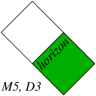
The causal structures of the BPS M-branes and D-branes are summarised in the Penrose diagrams in Fig.2. Note that the isotropic coordinates cover only part (shaded) of the maximally extended spacetime.

The F1 and NS5 spacetimes may be found by using the T- and S-duality formulæ that we gave in the last subsection.
3.2 Arraying BPS branes
Consider the BPS D-branes. They are described by the metric (3.5) with a single-centred harmonic function . In fact, BPS multi-centre solutions are also allowed because the equation for , , is linear:
| (3.7) |
The physical reason this works is that parallel BPS branes of the same kind are in static equilibrium: the repulsive gauge forces cancel against the attractive gravitational and dilatonic forces.
Let us make an infinite array of D-branes along the direction with periodicity . Define
| (3.8) |
then
| (3.9) |
Now, if , then the summand varies slowly with and we can approximate the sum by an integral. Changing variables to ,
| (3.10) |
we obtain
| (3.11) |
The quantity can be easily evaluated,
| (3.12) |
Then using we find
| (3.13) |
We can now take the limit that the arrayed objects make a linear density of branes. Then matching the thereby smeared harmonic function with the -brane harmonic function gives
| (3.14) |
We see that the linear density of -branes per unit length in string units becomes the number of -branes.
To check the identification we use the T-duality rules (2.53), with the isometry direction , to obtain
| (3.15) |
These agree with our expectations; they are precisely the supergravity fields appropriate to the D-brane.
The procedure of arraying the branes and then taking the limit is known as “smearing”; it results in a larger brane. Unsmearing, on the other hand, is in general difficult because dependence on the additional coordinate(s) must be reconstructed. In the case of a single type of D-branes we can guess and correctly get known results, but more generally guessing is not enough. In some cases with intersecting branes, unsmeared solutions do not exist, for good physics reasons [52].
Using dualities and our arraying formulæ we can of course interconnect all M-branes and D-branes with the NS-branes, W and KK. In working through this exercise, it is worth remembering that worldvolume directions are already isometry directions, and so in reducing along a worldvolume direction of a D-brane we have simply .
3.3 -brane probe actions and kappa symmetry
We would now like to consider what happens when we probe a D-brane spacetime, using another D-brane. We will treat the probe as a “test” brane, i.e. we will ignore its effect on the background geometry. This is a very good approximation provided that , the number of branes sourcing the spacetime, is large.
The action of a probe brane in a supergravity background has two pieces,
| (3.16) |
which are, to lowest order in derivatives,
| (3.17) |
where the are the worldvolume coordinates and denotes pullback to the worldvolume of bulk fields. The brane action encodes both kinetic and potential information, such as which branes can end on other branes [54, 55]. The WZ term, in particular, encodes the fact that D-branes can carry charge of smaller D-branes by having worldvolume field strength turned on.
Let us digress a bit on the structure of this action before we do the actual probe computation. The action we have written is appropriate for a brane which is topologically , and it also works for branes wrapped on tori. If the D-brane is wrapped on a manifold which is not flat, extra terms arise in the probe action. An example is the case of K3, where extra curvature terms appear [56], consistent with dualities.
Another interesting piece of physics which this action for a single probe brane does not capture is the dielectric or “puffing up” phenomenon of [57]. What happens there is that the presence of probe branes allows some non-commutative terms in the probe branes’ action which couple in to higher R-R form potentials. An example is the fact that D0-branes in a constant 4-form field strength background develop a spherical D2-brane aspect. For details on the modifications to the probe D-brane actions, the reader is referred to [57]. The full action for probe branes, which involves a nonabelian worldvolume gauge field, is in fact not known explicitly because the derivative expansion and the expansion in powers of the field strength can no longer be unambiguously separated. See the recent review [58].
The action possesses bulk supersymmetry, but not world-brane supersymmetry a priori. The gauge field lives on the branes, while the metric and -field are pullbacked to the brane in a supersymmetric way, e.g.
| (3.18) |
After fixing of reparametrisation gauge invariance and on-shell, there are twice too many fermionic degrees of freedom. This problem is familiar already from the Green-Schwarz approach to superstring quantisation [59]. The solution lies in an additional symmetry known as kappa-symmetry, a local fermionic symmetry which eliminates the unwanted fermionic degrees of freedom via a projection condition. In the case of Green-Schwarz quantisation of the superstring in a flat background, kappa-symmetric actions need a constant turned on. In light-front gauge, the projection condition which ensues is , and then via the equations of motion one sees that the erstwhile worldsheet scalars are in fact worldsheet spinors, and worldsheet supersymmetry then becomes manifest. See also the very recent important work of [60], in which a manifestly supersymmetric covariant quantisation of the Green-Schwarz superstring has been achieved.
A similar procedure works for the D-branes as well. In this case the DBI and WZ terms need each other in order to ensure kappa symmetry, all the while respecting bulk supercovariance. There is an intricate consistency [61] between kappa symmetry, the bulk supergravity constraints444Here we mean supergravity constraints in the technical sense; see e.g. [62]., and the bulk supergravity equations of motion. In a flat target space, the case of static gauge was worked out in [63]; the kappa symmetry can be used to eliminate and then the other spinor becomes the worldvolume superpartner of the gauge field and the transverse scalars. More generally, fixing the reparametrisation and kappa gauge symmetries to give manifest worldvolume SUSY is tricky. There has been some progress in spaces, see e.g. [64].
Now let us get back to using our test D-brane to probe the supergravity spacetime formed by a large number of the same type of brane. We have for the supergravity background the fields (3.5), which we repeat here for ease of reference,
The physics is easiest to interpret in the static gauge, where we fix the worldvolume reparametrisation invariance by setting
| (3.19) |
We also have the transverse scalar fields , which for simplicity we take to be functions of time only,
| (3.20) |
We will denote the transverse velocities as ,
| (3.21) |
Now we can compute the pullback of the metric to the brane.
| (3.22) |
The next ingredient we need is the determinant of the metric. To start, notice that
| (3.23) |
so that
| (3.24) |
Putting this together with the expression for the dilaton and the R-R field, we obtain
| (3.25) |
From this action we learn that the position-dependent part of the static potential vanishes, as it must for a supersymmetric system such as we have here. The constant piece is of course just the D-brane tension. In addition, we can expand out this action in powers of the transverse velocity. We see that, to lowest order,
| (3.26) |
and so the metric on moduli space, which is the coefficient of , is flat. This is in fact a consequence of having sixteen supercharges preserved by the static system.
3.4 Nonextremal branes
In string frame and with a Schwarzschild-type radial coordinate , the metric and dilaton fields of the nonextremal versions of the D-branes can be written as [32]
| (3.27) |
where
| (3.28) |
and the Hodge dual field strength for the R-R potential is directly proportional to the volume-form on the -sphere.
Defining
| (3.29) |
and making a change of coordinates to , the metric turns into a form more easily related to the extremal case we studied in the last subsection,
| (3.30) |
where
| (3.31) |
The other fields are
| (3.32) |
In these expressions, the boost parameter is given by
| (3.33) |
Notice in particular that in the extremal limit, where , . Alternatively, the change in the harmonic function due to nonextremality can be codified in a parameter :
| (3.34) |
Then we can express the gauge field as
| (3.35) |
The ADM mass per unit -volume and the charge are
| (3.36) |
The Hawking temperature and the Bekenstein-Hawking entropy are, respectively,
| (3.37) |
The extremal solution has degenerate horizons , and zero Bekenstein-Hawking entropy . The Hawking temperature of the extremal brane is also zero.
If we were to wrap this brane on a , then by the neat consistency of in various dimensions we discussed in section 1, the zero entropy result is also true of the R-R black hole. The volume of the torus at the horizon at extremality. This fact is related to zero entropy, via the field equations.
The causal structure of the uncompactified nonextremal D-brane can be found by noticing that the inner horizon is singular. The Penrose diagram in the plane then looks like that of a Schwarzschild black hole.
We close the discussion of the nonextremal D-brane solutions with a remark on supergravity -brane equations of state. For near-extremal -branes, the horizons are nearly degenerate. In this limit, , the function , and the only alteration of the metric due to nonextremality is the presence of . The relation between and the energy density above extremality is
| (3.38) |
The thermodynamic temperature and entropy are related to , which in the near-extremal limit is much smaller than the BPS D-brane tension, as
| (3.39) |
For general these relations are not familiar from any field theory. Disagreement between free field theory and supergravity entropies for these non-BPS systems is of course to be expected. There is however one notable exception, the case . In that case, a free massless gas gives entropy as a function of energy . Comparing this to the supergravity equations here, we see that the scaling agrees, with playing the role of the temperature . There is disagreement in detail [65], which comes from ignoring interactions [71].
Other nonextremal branes, such as NS5, can be obtained from the above D-brane solutions by duality transformations. We now move to discussion of a general instability afflicting nonextremal branes and black holes.
3.5 The Gregory-Laflamme instability
An important instability of nonextremal -branes was discovered in [66]. The simplest example of this phenomenon, which we now review briefly, occurs for neutral objects. We start with a neutral -dimensional black hole. It can come from a neutral configuration in dimensions in (at least) two different ways.
The first is from a black string, wrapped on compactified circle of radius ; and the second is from an array of -dimensional black holes, spaced by a distance . These are shown in Fig.3.

The array has to be infinite in order to get a static solution [67]. It well approximates the metric of the -dimensional black hole of interest if the perpendicular distances from the array are much larger than the spacing .
The question is then to find out which of the above configurations actually eventuates. Let us work in the microcanonical ensemble, which is appropriate for fixed energy (mass) of the system. The basic idea of the Gregory-Laflamme story is that whoever has the biggest entropy wins. The physics point is that the array of black holes has a different entropy than black string, because entropy is proportional to the area of the horizon, and spheres scale differently than cylinders. To see how it goes explicitly, let
| (3.40) |
For the black hole in dimensions, the properties of which we showed in detail in subsection 2.5 on solution-generating, we have
| (3.41) |
Therefore the mass per unit length of the array scales as
| (3.42) |
and since the masses must be equal we obtain
| (3.43) |
Now we can find which configuration has biggest entropy:
| (3.44) |
So the array dominates for small horizon radii, and the black string dominates for large horizon radii.
Sending , we see that the uncompactified neutral black string is always unstable. One can also see that this string is unstable by doing perturbation theory; there is a tachyonic mode, as shown in the original paper [66].
Note that the Gregory-Laflamme instability is different from the Hawking radiation instability. Let us now consider the possibility that when a neutral black string falls apart into an array of black holes, it violates the cosmic censorship hypothesis. In order for the cylindrically symmetric horizon of the string to break up into an array of spherical horizons, the singularity inside the black string horizon would have to go naked, at least for a while. In gravitational collapse, what may well happen instead is that the bits and pieces will collapse into the configuration preferred by the maximal entropy condition, obviating the need for temporary nakedness. However, in situations where the radius of the compact dimension varies dynamically in such a way that the string/array transition boundary is crossed, it is difficult to argue that violation of cosmic censorship does not occur.
The Gregory-Laflamme result does not imply instability of the uncompactified BPS charged -branes; there are several ways to see this. The first is that the tachyonic mode found for the neutral systems disappears in the extremal case; the length scale of the instability goes to infinity as the nonextremality parameter goes to zero. Another way to see it is that the BPS branes are protected by the Bogomolnyi bound. Consider what a BPS brane could break up into. A D-brane, for example, has a conserved charge, with even for Type IIA and odd for Type IIB. Therefore, if for example an uncompactified D1-brane wanted to break up into an array of D0-branes it would be out of luck because D0’s and D1’s do not occur in the same theory. If the D1 were wrapped on a circle, there would be a regime ()in which we should more properly describe it in the T-dual theory, i.e. as a D0. In this case the configuration is still stable, of course.
In our discussion of supergravity -branes, for simplicity we avoided those branes of dimension too large for them to be asymptotically flat. This was partly because they give rise to infrared problems, via logarithmic and linear potentials. We can however make one remark here about domain walls in the context of the Gregory-Laflamme instability. Domain walls separating different vacua of a theory will be stable even if they are neutral, because it would cost an infinite amount of energy for them to break up.
In this section we have been concerned with the properties of -brane geometries as classical spacetimes. More precisely, we were interested in semiclassical properties, such as Hawking radiation. Since the Hawking temperature is proportional to , the radiation is turned off in the limit. Also, since as all entropies are strictly infinite, one can argue that the Gregory-Laflamme instability is also absent in the classical limit. On the other hand, in the original paper exhibiting the tachyonic instability, the analysis was in fact classical. But since the dynamics of the instability requires the singularity to become naked while the horizon rearranges itself, the classical approximation is hardly a self-consistent analysis. It would be very interesting to apply the excision techniques of [68] in a numerical approach to understanding the Gregory-Laflamme instability.
We now move away from classical spacetimes by asking where they let us down.
4 When supergravity goes bad, and scaling limits
The supergravity actions such as (2.1) which we met in section 2 describe low-energy approximations to string theory. As such, they are appropriate for situations where corrections to the terms in them are small. In string theory, there are two expansion parameters which encode corrections to the lowest-order (supergravity) actions, namely the sigma-model loop-counting parameter and the string loop-counting parameter . Since is a dimensionful parameter, we need to fold it in with e.g. a measure of spacetime curvature in order to get a dimensionless measure of the strength of sigma-model corrections. The first corrections to the tree level IIA action shown above occur [69] at ; lower order corrections are prevented by supersymmetry. For the string loop corrections in the supergravity arena, we need the dilaton field, which typically varies in spacetime. The measure of how badly string loop corrections are needed is then .
We now discuss how string theory handles the breakdown of classical spacetime, in a few examples.
4.1 The black hole correspondence principle
The basic idea behind the Correspondence Principle is that stringy or braney degrees of freedom take over when supergravity goes bad.
The first example analysed was that of the -dimensional neutral black hole, which carries only mass. As discussed in subsection 2.5 on solution-generating, there is no dilaton so the Einstein and string metrics are the same,
| (4.1) |
where
| (4.2) |
Note that if we fix the mass and radius in units of , then the metric becomes flat as . (For simplicity we taken the volume of any internal compact dimensions to be of order the string scale. The actual value does not affect the argument.)
The supergravity black hole solution breaks down in the sense of the correspondence principle [71] when curvature invariants at the horizon are of order the string scale. The physical reason why we concentrate on the horizon, rather than the singularity, is that its presence is what signals the existence of a black hole. Using the horizon also gives rise to sensible answers which fit together in a coherent fashion under duality maps. A curvature invariant which is nonzero for the neutral black hole is , so that breakdown of supergravity occurs when
| (4.3) |
The thermodynamic temperature and entropy of the black hole scale as
| (4.4) |
so the Hawking temperature at the correspondence point (4.3) is .
The simplest string theory object which carries only the conserved quantum number of mass is the closed fundamental string. We will therefore be interested in seeing if we have a fundamental string description where the black hole description breaks down. (One reason why we choose the simplest object, rather than say a spherical D2-brane, is Occam’s razor. It is also important that the correspondence point occurs at which involves no powers of .) In fact, the idea that black holes might be fundamental strings dates back to the late ’60’s. The idea was put on a firmer footing by Sen [70] and Susskind [23] before the duality revolution. The subsequent formulation of the Correspondence Principle made those ideas more powerful. One of the ways it did this was to recognise that black holes and string states typically do not have identical entropy for all values of parameters; rather, the transition between black hole and string degrees of freedom occurs at a transition point, known as the Correspondence Point. The existence of a correspondence point for every system studied is a highly nontrivial fact about string theory and the degrees of freedom that represent systems in it in different regions in parameter space.
To progress further, we now need the statistical entropy of closed string states due to the large degeneracy at high mass. This is a standard result in perturbative string theory so we will not review it here but refer to the texts [39, 59]. We assume that the string coupling is weak so that we can use the free spectrum computation; this assumption will be justified a posteriori.
Using the relation between the oscillator number and the mass , , we have for the closed superstring degeneracy of states at high mass,
| (4.5) |
With better approximation schemes, one can keep track of power-law prefactors that depend on the number of large dimensions. We have suppressed these because they are not important at large-.
The quantity is the Hagedorn temperature. At the Hagedorn temperature, the canonical ensemble is in fact no longer well-defined. This happens because the partition function diverges,
| (4.6) |
At the Hagedorn temperature, the excited string becomes very long and floppy. The Boltzmann entropy of the string state is the log of the degeneracy of states,
| (4.7) |
Matching the masses at the correspondence point for general Schwarzschild radius yields
| (4.8) |
This gives the general entropy ratio
| (4.9) |
We can see four pieces of physics from this formula. Firstly, the crossover from the black hole to string state indeed happens at , as suggested earlier. Secondly, the black hole dominates for i.e. for large mass, while the string dominates at lower mass. Thirdly, let us calculate the string coupling at the correspondence transition point. Since the entropy at correspondence is , and , we get . Also, we have the formula . From this we find that at transition. This is indeed weak coupling since is very large. This justifies our earlier assumption that we could calculate the string degeneracy by using weak-coupling results. Lastly, note that in general , the mass at correspondence is not the Planck mass .
More work has been done on the physics of the transition between the black hole and the string state. The interested reader is referred to e.g. [72, 73] and references therein.
We have seen that the black hole and string state entropies match in a scaling analysis at the correspondence point. The physics implications of the correspondence principle run even deeper, however. The conservative direction to run the matching argument tells us that a string state will collapse to a black hole when it gets heavy enough. The radical direction to run the argument is the other way: the correspondence principle is in fact telling us that the endpoint of Hawking radiation for a Schwarzschild black hole is a hot string. The hot string will then subsequently decay by emitting radiation until we are left with a bath of radiation. An interesting fact about this decay of a massive string state in perturbative string theories is that the spectrum is thermal, when averaged over the degenerate initial states [74].
Overall, we see that the picture of decay of a Schwarzschild black hole in string theory is in tune with expectations that a truly unified theory should not allow loss of quantum coherence.
4.2 NS-NS charges and correspondence
The work of Sen [70] on comparing entropy of BPS black holes and the corresponding string states predated the correspondence principle, but the results can in fact be considered as additional evidence for it.
Black holes with two NS-NS charges in dimensions can be constructed using the solution-generating technique [75]. Taking the BPS limit is straightforward, and the Bekenstein-Hawking entropy is easily obtained. One hiccough that occurs is that the entropy of the classical BPS black holes is zero, because the area of the horizon is zero. However, as argued by Sen, [70], higher order corrections to the equations of motion will modify this, and make the area of the horizon become of order string scale rather than zero. This results in a finite entropy, which can be compared to the entropy of the stringy state because the system is BPS and there is a nonrenormalisation theorem for the degeneracy of states.
The next step is to identify which stringy state the black hole will turn into at the correspondence point. Consider the deviation of the geometry from Minkowski spacetime, as we did for the neutral black holes. Corrections to the flat metric go like , and as this scales to zero with the Newton constant. (We have assumed that no compactified directions scale to zero as a power of .) From this, we can then guess that the black hole will turn into a perturbative string state at the correspondence point. In particular, the BPS black holes correspond to states of the fundamental string with both momentum and winding charge, wound around a circle. The degeneracy of states formula is well known and can be easily compared to the Bekenstein-Hawking entropy of the black holes. It is in scaling agreement with the entropy coming from the statistical degeneracy of states of the closed string with the same quantum numbers [70, 75].
For the case of NS5-brane charge, the physics is more tricky. The reason is related to how deviations from the flat metric scale with for the different branes. Above, we saw how BPS black holes carrying string-like charges turned into string states at the correspondence point, which occurred at weak coupling. An analogous phenomenon is not possible for NS5-branes. We can see this from combining the scalings (2.29) in the Bogomolnyi bound with the generic equation for the deviation from the flat metric, for some appropriate to the brane. Since Newton’s constant scales as at fixed , any brane with an scaling with two or more negative powers of will not approach the flat metric as the string coupling is scaled to zero. The F1 and D have respectively, but the NS5 has and so it is out of luck. We do not have space here to discuss the physics of what replaces the supergravity NS5-brane in regions of parameter space where the supergravity solution goes bad, but the question has been investigated in limits different to ; see e.g. [76, 77].
Quite generally, though, in order to apply the correspondence principle, we must identify the microscopic degrees of freedom that will take over from the supergravity description when it breaks down, i.e. where the curvature at the horizon or the dilaton gets too large. There are two important criteria which these stringy/braney degrees of freedom must fulfil: they must have same conserved quantum numbers, and they must be localised near the would-be black hole at the correspondence point. The second condition is needed in order to prevent counting of the wrong states, e.g. we would not count closed strings far outside the would-be Schwarzschild radius in our original example of the neutral black hole.
We now move to the case of R-R charged systems.
4.3 Where BPS D-branes go bad
Let us begin our discussion of the case with one R-R charge with an analysis of where the supergravity solutions break down. The Ricci scalar is nonzero in the D-brane spacetimes, and we find
| (4.10) |
Let us consider the behaviour of this as . Since the harmonic function near , we have
| (4.11) |
This blows up for the big -branes, i.e. those with . In addition, we know that the curvature is zero at infinity, and rises as we come in from infinity. Therefore the curvature is non-monotonic for branes with . The information on the curvatures for branes is summarised in Fig.4.
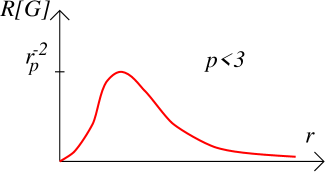
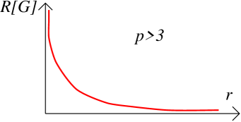
The dilaton behaves differently. We have
| (4.12) |
This blows up at for the small branes, i.e. for . The slope for the dilaton is monotonic, but for there is an inflection point. We summarise this information in Fig.5.
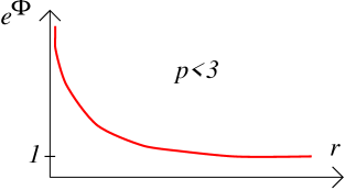
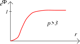
Note the interesting fact that, if the asymptotically flat part of the geometry is removed by losing the constant piece (the 1) in the harmonic function, then the behaviour of both the curvature and the derivative of the dilaton becomes monotonic. This turns out to be a crucial supergravity fact in the context of the D-brane gravity/gauge correspondences of [76].
In our brief discussion of the NS5-brane in the last subsection, we saw that the D-brane supergravity solutions do approach a flat metric as at fixed . By following the conserved quantum numbers, we therefore see that the weak-coupling degrees of freedom are D-branes in their perturbative incarnation as hypersurfaces where fundamental strings end.
If we then compactify the D-branes on , we find R-R black holes. By the structure of Kaluza-Klein reduction formulæ, we can see that the resulting supergravity geometries blow up at . R-R black holes in with one charge are of course partnered with wrapped perturbative D-branes [71] .
In this system, the energy above extremality can be carried by either open or closed fundamental strings, as long as they are close to the D-branes. Open and closed strings have different equations of state. Again, we assume weak string coupling; this assumption can be justified a posteriori. For the open strings, assuming a free massless gas yields
| (4.13) |
while for the closed strings the equation of state is
| (4.14) |
It is found that open strings dominate for near-extremal black holes, while closed strings dominate for far-from-extremal black holes as happened in our neutral black hole example. In addition, the correspondence points of the single-charge NS-NS and single-charge R-R black holes are related by duality and they match up. This is a general phenomenon; also, in a highly nontrivial fashion it meshes nicely with the Gregory-Laflamme transition [71].
In terms of advances in precise computations of black hole entropy, the most important examples of the application of the correspondence principle are systems with two or more R-R charges. This is the case both for the BPS and the near-BPS black holes. The crucial physics observation is that for these systems, the scaling works in such a way that there is no correspondence point, and so exact comparisons can be made to weak-coupling stringy/braney calculations for black holes of any horizon radius. We will discuss the spectacular success of these microscopic calculations in later sections.
4.4 Limits in parameter space, and singularities
In figuring out what degrees of freedom replace a fundamental string or D-brane supergravity geometry when it goes bad, we discussed the limit of the system. More generally, the idea of taking limits of parameters, in the context of the correspondence principle and otherwise, has yielded very powerful results. These results have taught us very interesting facts about gravity and about gauge theories, including non-commutative gauge theories.
A limit of D-brane systems which has been used to great effect is the decoupling limit, in which interactions between the open strings ending on the branes and the closed strings in the bulk are turned off. The resulting gravity/gauge correspondences are the domain of other Lecturers at this School, but we cannot resist a few remarks here. The main physics behind the limit is to take string tension to infinity, while holding some physically interesting parameters fixed. It can be confusing to scale dimensionful quantities to zero, so we work with dimensionless quantities here. In units of a typical energy of the system, taking the string tension to infinity is then expressed as . In order to retain a finite -dimensional gauge coupling on the branes, we hold fixed . Also held fixed is the energy of open strings stretched between different D-branes separated by distance , i.e. . In the decoupling limit, by definition, the bulk theory and the brane theory are each a unitary theory on their own. Maldacena [78] argued (initially for certain systems) that the two theories are actually dual to one another. This idea has been extended to many other systems, in e.g. [76], goes by the name of the gravity/gauge correspondence, and is very powerful.
Assuming that the gravity/gauge correspondence (conjecture) is true for all values of loop-counting parameters, then it provides an explicit realization of information return. It does this because any process of black hole formation and evaporation in the supergravity theory has a dual representation in the unitary quantum field theory. It is, however, extremely difficult to see how information return works in practice [29], because the duality between the gravitational theory and the gauge theory is a strong-weak duality. The issue of how a semiclassical spacetime picture emerges from the strongly coupled gauge theory, with (approximate) locality and causality built in, is one of the most interesting and important challenges of this field of study.
In the decoupling limit, the supergravity D-brane geometry loses its asymptotically flat part, as can be seen by plugging the above scalings into the equation (3.6) for the harmonic function. (Also, the worldvolume coordinates on the brane are the same as the , which are the supergravity worldvolume coordinates in the asymptotically flat region of the original D-brane geometry.) So, let us consider the near-horizon geometry of the -branes. Abbreviate
| (4.15) |
and look at the geometry for , i.e. let us ignore the 1 in the harmonic function for the D-brane geometry. Changing to a coordinate
| (4.16) |
for the BPS systems yields the structure
| (4.17) |
which gives a geometry conformal to [79]. The z-dependent prefactor disappears only for . Since the asymptotically flat part of the geometry is gone in the decoupling limit, the Penrose diagrams are drastically altered.
In addition, as we saw in our analysis of where D-branes go bad, the curvature and the dilaton behave monotonically with radius when the 1 is missing from the harmonic function. Combining the supergravity and brane field theory information in the decoupling limit leads to the construction of the phase diagram [76] for the D-brane system. A nice discussion of phase diagrams in more generality can be found in [80]. More recent considerations which include the physics of turning on a -field (noncommutativity), with emphasis on , may be found in [81]. For the non-BPS systems, the only deviation from the BPS metric in the decoupling limit is the nonextremality function (the function in eqn (3.31)) which multiplies . One way to see that the function is unmodified from the BPS case is to combine the decoupling limit scalings with the equation for the energy density above extremality , given in (3.38), with the relation for the boost parameter (3.33).
To finish this section on where supergravity brane geometries go bad, we now make a few remarks about classical curvature singularities.
In the discussion of the correspondence principle, for cases with separate horizon and singularity, we used the curvature at the horizon to determine where the supergravity solution broke down. The question of what happens at the singularity is also, of course, a question of physical interest in string theory. The general expectation might be that string theory smoothes out regions of classically infinite curvature.
However, Horowitz and Myers [82] made the important point that some singularities are not of the kind that can be smoothed out because this would give rise to a contradiction. The prototypical example is the negative-mass Schwarzschild geometry. Since , the horizon is absent, so the singularity is naked. If the singularity were smoothed out by stringy phenomena, the resulting finite-sized blob would be an allowed object with overall negative mass. It would then destabilise the vacuum - via pair production, for example. The upshot is that the negative-mass Schwarzschild geometry is a figment of the classical physicist’s imagination.
It is also important to note that the question of whether a geometry is singular depends on the dimension of the supergravity theory it is embedded in. For example, in [83], it was shown that some lower-dimensional black holes with singularities could be lifted to nonsingular solutions in higher dimensions. For understanding possible resolution of singularities in terms of basic stringy objects like D-branes, the best dimension to do the singularity analysis is , which is the dimension in which D-branes naturally live. It is generally more confusing to try to do the analysis directly in lower dimensions. In addition, one should be sure that any operation one does in supergravity also makes sense in string theory.
There are spacetimes in string theory with singularities, such as the fundamental string and the gravitational wave, which appear to be exact solutions to all orders in . In [36] it was, however, argued that forgotten source terms in the action actually do lead to corrections, which smooth out these singularities. For the string, we can in any case think of the singularity of the classical geometry as smoothed out by the source which is the fundamental string itself [50]. In addition, for the D-branes, the phase diagrams of [76] show that a gauge theory takes over in regions where the classical geometry has a (null) singularity. This provides an understanding of singularity resolution in these systems, which possess supersymmetry in language.
A more recently discovered phenomenon known as the enhançon mechanism has provided a stringy resolution of some classical timelike naked singularities [84]. The essential physics behind this is that string theory knows what to do when certain cycles on which D-branes are wrapped become small; previously irrelevant degrees of freedom become light and enter the dynamics. Put this way, the enhançon phenomenon may in fact be quite general; work on more applications is in progress.
5 Making black holes with branes
Black holes in string theory with macroscopically large entropy can all be constructed out of various -brane constituents. We concentrate in this section mostly on BPS systems where the rules are simplest.
5.1 Putting branes together
Two clumps of parallel BPS -branes are in static equilibrium with each other. In addition, BPS -branes and -branes for some choices of can be in equilibrium with each other under certain conditions. One way to find many of the rules is to start with the fundamental string intersecting a D-brane at a point.
By T- and S-duality, we can infer the following NS5-, F1-, and D- brane intersections. We use the convention that an -type object intersecting a -type object in spatial dimensions is represented by or , depending on whether and are parallel or perpendicular to each other. In this notation, our fundamental string/D-brane intersection is denoted F1D. We then get via dualities
| (5.1) |
For simplicity we have restricted to -branes whose geometries are asymptotically flat. (We have also only listed pairwise intersections for the same reason; multi-brane intersections must obey the pairwise rules for each pair.) In the rules are
| (5.2) |
This leads to a set of rules for putting W and KK on branes. Recall that for KK, whose spacetime metric was displayed in eqn.(2.69), one of the four transverse directions is singled out as the isometry direction while the metric depends on the other three coordinates. Because not all perpendicular directions are equivalent, the KK intersection rules are rather involved; see for example [85].
For some brane intersections not displayed above, there is an additional complication which arises upon careful consideration of force cancellation, via closed string tree or open string 1-loop amplitudes. The prototypical example is the case of a D0-brane and a D8-brane. When the D0-brane crosses the D8-brane, a fundamental string is created; the physics requires this to happen for force cancellation to be preserved. A dual situation where this occurs is in the Hanany-Witten setup where a D3-brane is created when a D5-brane crosses an NS5-brane. For a pedagogical discussion of this brane creation story we refer the reader to [86].
5.2 Intersection-ology à la supergravity
The simplest system to study is supergravity, and studying the action for the theory gives rise to the intersection rules for M-branes. The action for the gauge potential in the bosonic sector is
| (5.3) |
The constant can be changed by a field redefinition. The field strength is defined as
| (5.4) |
and so it obeys a Bianchi identity
| (5.5) |
This implies that the charge
| (5.6) |
is conserved, where the integral is over a transverse four-sphere. This is the M5-brane charge. The Bianchi identity also implies that the M5-brane cannot end on anything else. It can, however, have a funny-shaped worldvolume pointing in different directions.
Then, with a convenient normalisation of #, the field equation for is
| (5.7) |
where we used the Bianchi identity. This tells us that the conserved charge, this time the M2-brane charge, is
| (5.8) |
Consider the M2-brane ending on something. To picture this, suppress one of its dimensions and also several of those of the object on which the M2 ends. In fact, the surface on which the M2 ends must be the M5, because nothing else carries . A diagram is shown in Fig.6.
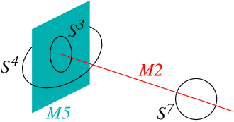
Far from the boundary, only the piece in the charge matters, and so is indeed the membrane charge. On the other hand, right at (and only at) the place where the M2 ends on the M5, we can deform . In addition, the components of the field strength parallel to the M5-brane are approximately zero there, because the flux threads the in a spherically symmetric way. As a consequence, on the M5, one can write the approximate relation , for some two-form . Then the charge factories into
| (5.9) |
The first factor is the (magnetic) charge of the string which is the boundary of the M2-brane in the M5-brane worldvolume. This leads to the rule M2M5(1).
This procedure can be generalised to find other brane intersection rules in other supergravity theories in various dimensions [88].
5.3 Making BPS black holes with the harmonic function rule
BPS black holes in dimensions may be constructed from BPS -brane building blocks. Typically, however, they have zero horizon area and therefore non-macroscopic entropy. The essential reason behind this slightly annoying fact may be distilled from the supergravity field equations [3]. The sizes and shapes of internal manifolds, as well as the dilaton, turn out to be controlled by scalar fields, and the horizon area is related to these scalars. But in any given dimension , there are only a few independent charges on a black hole, and mostly these give rise to too few independent ratios to give all the scalar fields well-behaved vevs everywhere in spacetime. For stringy black holes made by compactifying on tori, the only asymptotically flat BPS black holes with macroscopic finite-area occur with 3 charges in and 4 charges in [89]. For a survey of supergravities in various dimensions and the kinds of black objects that can carry various central charges, relevant to D-brane comparisons, see [90, 91].
A systematic ansatz [92] is available for construction of supergravity solutions corresponding to pairwise intersections of BPS branes, which is known as the “harmonic function rule”. The ansatz is that the metric factories into a product structure; one simply “superposes” the harmonic functions. This ansatz works for both parallel and perpendicular intersections, using the construction rules we reviewed in the last subsection, with the restriction that the harmonic functions can depend only on the overall transverse coordinates. In this way we get only smeared intersecting brane solutions. Let us discuss some examples.
We use a convention where indicates that the brane is extended in a given dimension, indicates that it is pointlike, and indicates that, although the brane is not extended in that direction a priori, its dependence on those coordinates has been smeared away. As an example, consider a D5 with a (smeared) D1:
| (5.10) |
and D2 perpendicular to D2’ (both smeared):
| (5.11) |
For the D1-D5 system, let us define to be the overall transverse coordinate in the setup above in eqn.(LABEL:d5sd1). Then the string frame metric is, using the harmonic function rule,
| (5.12) |
and dilaton is
| (5.13) |
while the gauge fields are as before,
| (5.14) |
The independent harmonic functions both go like in the interior, which is natural for a D5-brane and also for a D1-brane smeared over four coordinates:
| (5.15) |
Notice that if we wrap on , in order to make a black hole with two charges, the volume of the is finite at the event horizon :
| (5.16) |
However, if we compactify the direction along the string, , on a circle, the radius goes to zero at the event horizon no matter how large its value at infinity:
| (5.17) |
In addition, the area of the event horizon in Einstein frame, and therefore the entropy, is zero.
It is interesting to note that not all known supergravity solutions for intersecting branes are smeared or delocalised in this way. The factorised metric ansatz works in some other situations as well. E.g. let depend on , and on , and let depend on . The equations of motion are found to be, see e.g. [93],
| (5.18) |
Therefore is as before in the smeared case, but has extra dependence, on the coordinates parallel to the D5-brane but perpendicular to the D1-brane. cannot be written in terms of elementary functions but can be written as a (-)Fourier transform of known functions. This is the case even with transverse separations between the D1’s and D5’s. More generally, there is an interesting delocalisation phenomenon which occurs as the transverse separation between a D-brane and a D-brane to which it is parallel goes to zero. Delocalisation is found to occur only for ; an explanation of these phenomena in the context of the AdS/CFT correspondence was found. Some localised solutions are known analytically near the horizon of the bigger brane, and for some intersecting brane systems the factorised ansatz is not sufficient. For a discussion of the above issues see [52], and for recent advances in constructing localised intersecting M5-brane solutions in see [53].
5.4 The 3-charge black hole
We saw in the previous subsection that a black hole with only D1- and D5-brane charges does not have a finite horizon area. We can now use our knowledge from solution-generating to puff up this horizon to a macroscopic size by using a boost in the longitudinal direction .
The ingredients for building this black hole are then the previous branes with the addition of a gravitational wave W:
| (5.19) |
The indicates the direction in which the gravitational wave W moves (at the speed of light).
The BPS metric for this system is obtained from the simpler metric for the plain D1-D5 system by boosting and taking the extremal limit. To get rid of five dimensions to make a black hole, we then compactify the D5-brane on a of volume , and then the D1 and the remaining extended dimension of the D5-brane on a of radius . The Einstein frame metric becomes
| (5.20) |
where the harmonic functions are
| (5.21) |
and using arraying for and we find
| (5.22) |
This supergravity solution has limits to its validity. If the stringy corrections to geometry are to be small, we need the curvature invariants small. Supposing that we keep the volumes fixed in string units, this forces the radius parameters to be large in string units, . We can also control string loop corrections if . These two conditions are compatible if we have large numbers of branes and large momentum number for the gravitational wave W. Note from the relations (5.22) that for all ’s of the same order hierarchically, , while for , and small, . On the other hand, if we want of the same order, must be hierarchically large: .
The next properties of this spacetime to compute are the thermodynamic quantities. The BPS black hole is extremal and it has . For the Bekenstein-Hawking entropy,
| (5.23) |
This entropy is macroscopically large. Notice that it is also independent of and of . This is to be contrasted with the ADM mass
| (5.24) |
which depends on explicitly.
For the entropy of the black hole just constructed out of D1 D5 and W, we had . More generally, for a more general black hole solution of the maximal supergravity arising from compactifying Type II on , it is
| (5.25) |
where the quantity in the surd is the cubic invariant of the duality group,
| (5.26) |
and are the eigenvalues of the central charge matrix .
A few years ago the claim was made, via classical topological arguments in Euclidean spacetime signature, that all extremal black holes have zero entropy. This result is not trustworthy in the context of string theory. For starters, as we mentioned in our discussion of the Third Law, there is no physical reason why zero-temperature black holes should have zero entropy. In any case, the faulty nature of the classical reasoning in the string theory context was pointed out in [2]. In the Euclidean geometry, for any periodicity in Euclidean time at infinity, the presence of the extremal horizon results in a redshift which forces that periodicity to be substringy very close to the horizon. Since light strings wound around this tiny circle can condense, a Hagedorn transition can occur and invalidate the classical approximation there. In fact, other Hagedorn-type transitions can come into play when spatial circles get small near a horizon, as they do e.g. for -branes compactified on tori [94].
5.5 The 4-charge black hole
The extremal Reissner-Nordström black hole can be embedded in string theory using D-branes. Recall that in the extremal spacetime metric (1.18) we had ’s appearing in the metric. This is to be contrasted with the ’s to be found in a generic -brane metric. From this we can guess (correctly) that, in order to embed the extremal RN black hole in string theory, we will need 4 independent brane constituents. Restrictions must be obeyed, however, in order for that black hole to be RN. To make more general black holes with four independent charges, we simply lift these restrictions and allow the charges to be anything - so long as they are large enough to permit a supergravity description.
For making the black hole, one set of ingredients would be
| (5.27) |
By U-duality, we could consider instead 4 mutually orthogonal D3-branes, or indeed many other more complicated arrangements [96].
In ten dimensions we can construct the BPS solution by using the harmonic function rule. So far we have not exhibited the metric for the NS5-branes but that can be easily obtained using the D5 metric and using the fact that the Einstein metric (2.7) is invariant under S-duality. We then have
| (5.28) |
and
| (5.29) |
After arraying till we are blue in the face, and finding Newton’s constant using
| (5.30) |
we get for the gravitational radii
| (5.31) |
We now use our Kaluza-Klein reduction formulæ to reduce to the black string,
| (5.32) |
In this process, the dilaton gets some factors:
| (5.33) |
Using our KK formula , we find upon reducing on the last direction
| (5.34) |
The dilaton gets changed again:
| (5.35) |
Finally the Einstein metric in is
| (5.36) |
The Bekenstein-Hawking entropy is then easily read off to be
| (5.37) |
More generally, in the surd is the quantity , where is the quartic invariant of [95],
| (5.38) |
where are the (complex) eigenvalues of ; see e.g. [91, 96]. More recent further progress on entropy-counting for these black holes may be found in [97].
The connection to the Reissner-Nordström black hole is obtained by setting all four gravitational radii to be identical: .
Although we have not discussed nonextremality explicitly here, it can be achieved by adding extra energy to the system of branes. Generic nonextremal branes cannot be in static equilibrium with each other, as they typically want to fall towards each other, and they do not satisfy the simple harmonic function superposition rule. The least confusing way to construct nonextremal multi-charge solutions is to start with the appropriate higher- neutral Schwarzschild or Kerr type solution, and to use multiple boostings and duality transformations to generate the required charges.
6 BPS systems and entropy agreement
In this section we review the D-brane computation of the entropy of BPS systems with macroscopic entropy, with its many facets. For BPS systems there is a theorem protecting the degeneracy of states, and so the entropy computed in different pictures will agree.
6.1 The Strominger-Vafa entropy matching:
Since we have already built the black holes with the relevant D1 and D5 charges, and worked out their macroscopic Bekenstein-Hawking entropy, we turn to the microscopic computations of the entropy from the string theory point of view. We will discuss the D-brane method of [98] (earlier ideas for a microscopic accounting for of BPS black holes [99] with macroscopic entropy included [100]). A more detailed review of some aspects of the D1-D5 system can be found in the recent lecture notes of [101].
Our setup of branes was
| (6.1) |
This system preserves 4 real supercharges, or in . This can be seen from the constituent brane SUSY conditions; each constituent breaks half of SUSYs. It is necessary for SUSY to orient the branes in a relatively supersymmetric way; if this is not done, e.g. if an orientation is reversed, the D-brane system corresponds to a black hole that is extremal but has no SUSY.
By using D1- and D5-brane ingredients we have two kinds of quantum number so far, and . The degrees of freedom carrying the remaining momentum number, and the angular momentum, are as yet unidentified. Now, the smeared D1-branes plus D5-branes have a symmetry group . This symmetry forbids the (rigid) branes from carrying linear or angular momentum, and so we need something else. The obvious modes in the system to try are the massless 1-1, 5-5 and 1-5 strings, which come in both bosonic and fermionic varieties. The momentum is indeed carried by the bosonic and fermionic strings, in units of . The angular momentum is carried only by the fermionic strings, each. Both the linear and the angular momenta can be built up to macroscopic levels.
The next step is to identify the degeneracy of states of this system. The simplification made by [98] is to choose the four-volume to be small by comparison to the radius of the circle,
| (6.2) |
so that the theory on the D-branes is a theory. This theory has SUSY.
Because the D1-branes are instantons in the D5-brane theory, the low-energy theory of interest is in fact a -model on the moduli space of instantons . The central charge of this theory is . Roughly, this central charge can be thought of as coming from having 1-5 strings that can move in the 4 directions of the torus. Alternatively, can be thought of as roughly coming from having instantons in the gauge theory, and orientations to point them in.
The other ingredient needed to compute the degeneracy of states, apart from the central charge, is the energy. Now, since the system is supersymmetric, we have to put the right-movers in their groundstates. The left-movers, however, can be highly excited. Since the excited states are BPS in dimensions, their energy and momentum must be related by .
The partition function of this system is the partition function for bosons and an equal number of fermions
| (6.3) |
where is the degeneracy of states at energy . At large- we can use the Cardy formula
| (6.4) |
This formula assumes that the lowest eigenvalue of the energy operator is zero, as it is in our system. (Otherwise we would need to subtract from to get the effective central charge, where is the ground state energy).
Therefore the microscopic D-brane statistical entropy is
| (6.5) |
This agrees exactly with the black hole result.
Subleading contributions to both the semiclassical Bekenstein-Hawking black hole entropy and to the stringy D-brane degeneracy of states have been calculated, both on the black hole side and on the D-brane side, and they have been found to match. See for example the beautiful work of [102]. At this point we mention that there is another method using M-theory available for counting the entropy of these black holes, as discussed in [103], which we do not have space to cover here.
6.2 Rotation
In there are two independent angular momentum parameters, because the rotation group transverse to the D1’s and D5’s splits up as . The metrics for general rotating black holes are algebraically rather messy and we will not write them here. We will simply quote the result for the BPS entropy [48]:
| (6.6) |
The BPS black holes have a nonextremal generalisation, in which the two angular momenta are independent. However, in the extremal limit something interesting happens: the two angular momenta are forced to be equal and opposite, . There is also a bound on the angular momentum,
| (6.7) |
Beyond , closed timelike curves develop, and the entropy walks off into the complex plane. Another notable feature of this black hole is that the funny cross-terms in the R-R sector of the supergravity Lagrangian like (2.1) are turned on; this black hole is not a solution of Einstein-Maxwell theory. The charges are, however, unmodified by the funny cross-terms which fall off too quickly at infinity to contribute.
Let us now move to the D-brane field theory. It is hyperKähler due to supersymmetry, so let us break up the into left- and right-moving superconformal algebras, each of which has a subgroup. The corresponding charges can be identified [48] as:
| (6.8) |
Recall that the BPS system is in the R-moving groundstate, and at left-moving energy . These facts give rise to a bound on w.r.t. . The essential physics behind this is simply that in order to build angular momenta we have to spend oscillators, and for a fixed energy our funds are limited. For the details let us bosonise the currents:
| (6.9) |
where is the complex dimension of , i.e. . Then a state with charge is represented by an operator
| (6.10) |
where an operator from the rest of the CFT. The construction is entirely similar for . Now, the operator has positive dimension overall, so we get a bound on the charges
| (6.11) |
Since the R-movers are in their groundstate, is small and fixed. However, can be macroscopically large. In the supergravity description we are only sensitive to macroscopic quantities, and so we will be unable to ‘see’ , only . Since the angular momenta are the sum and difference of and respectively, as in (6.8), we find agreement with the black hole result in the BPS limit: .
The next item on the agenda is to compute the effect of the angular momenta on the D-brane degeneracy of states. We had that the total eigenvalue of is . However, we spent some of this, , on angular momenta. So the available for making degeneracy of states is
| (6.12) |
Notice that for small we have an excitation energy gap
| (6.13) |
Then the microscopic entropy is
| (6.14) |
This again agrees explicitly with the black hole calculation.
6.3 Fractionation
An important subtlety arises in the use of the exponential approximation to the degeneracy of states formula. The approximation is valid only for energies such that is large; this turns out to be true only for . We may ask what goes wrong if all are of the same order.
The simplest way to see the approximation break down physically is to picture [104] the left-movers as a gas of 1-5 strings, with order massless species of average energy . Let us introduce a temperature for the left-movers. Note that doing this does not screw up supersymmetry of the system, because the BPS condition is a condition on right-movers. The BPS system simply has zero right-moving temperature. It is legitimate to have different temperatures for left and right movers because there is a net momentum.
Assuming extensivity gives
| (6.15) |
and entropy
| (6.16) |
Eliminating between these relations gives
| (6.17) |
as required. However, substituting back to find we find
| (6.18) |
i.e. the inverse temperature is longer than the wavelength of a typical quantum in a box of size . So our gas is too cold for thermodynamics to be applicable, and we cannot trust our equations.
In fact, if the three are of the same order, then the strings “fractionate” [104]. A recent analysis [105] of the physics of this system in a CFT approach has yielded a rigorous explanation of fractionation. As an example of the basic idea, consider ; what happens is that the D1’s join up to make a long string, as shown in Fig.7.

Then the energy gap, instead of being , is , which is much smaller. As a consequence, there are now plenty of low-energy states. Notice that this is the same gap as we saw above in our study of rotation. With the smaller gap, we have just one species instead of species, and the energy is
| (6.19) |
The entropy is
| (6.20) |
Therefore, the temperature is as before,
| (6.21) |
but this time it is plenty hot enough for the equation of state to be valid because the box size is bigger by a factor of .
The entropy counting now proceeds in a similar manner as before, but the central charge and the radius are modified as and . The result is identical.
6.4 entropy counting
A canonical set of ingredients for building the system is what we had previously in building the black hole:
| (6.22) |
The new feature of this system compared to the previous one is that D2-branes can end on NS5-branes. It costs zero energy to break up a D2-brane as shown in Fig.8.

These extra massless degrees of freedom in the system lead to an extra label on the 2-6 strings, giving rise to an extra factor of in the degeneracy. The entropy counting proceeds just as before, and yields [106]
| (6.23) |
which again agrees exactly with the Bekenstein-Hawking black hole entropy. A major difference between this and the case is that rotation is incompatible with supersymmetry; in addition, there can be only one angular momentum .
7 Non-BPS systems, and Hawking radiation
Among black holes and black branes, BPS systems are the systems under the greatest theoretical control because supersymmetry implies the presence of nonrenormalisation theorems for quantities including entropy. Their non-BPS counterparts are also very much worthy of study and we now turn to a discussion of their properties.
7.1 Nonextremality
The nonextremal black hole metric for the D1 D5 W system comes from the string frame metric
| (7.1) |
where
| (7.2) |
and ’s are the boost parameters used to make this solution. The conserved charges are given by
| (7.3) |
and the mass and thermodynamic quantities are
| (7.4) |
In the limit
| (7.5) |
the expression for the ADM mass simplifies; the energy above extremality becomes
| (7.6) |
We also had that
| (7.7) |
now define
| (7.8) |
From this we can see that the system has effectively split into independent gases of left- and right-movers:
| (7.9) |
This regime is dubbed the “dilute gas regime” because the energies and momenta are additive. This regime is, in fact, exactly what is selected by taking the decoupling limit we discussed in section (4).
Let us proceed to compute the Bekenstein-Hawking entropy. In the dilute gas limit (7.5), the only boost parameter which is still effectively non-infinite is . The entropy is then proportional to
| (7.10) |
The dilute gas entropy becomes [107]
| (7.11) |
Thus the entropy is additive. By very similar calculations as before we can see that the D-brane entropy counting gives exactly the same result as the Bekenstein-Hawking entropy in the dilute gas regime. For the nonextremal system the agreement persists even with the introduction of rotation [108]. In the case of the four-charge black holes, similar results ensue [109].
We may ask at this stage why the entropy of these near-extremal supergravity and perturbative D-brane systems agree, as there is no theorem protecting the degeneracy of non-BPS states. What is going on physically is that conformal symmetry possessed by the theory is sufficiently restrictive, even when it is broken by finite temperature, for the black hole entropy to be reproduced by the field theory.
7.2 The BTZ black hole and the connection to D1-D5
In three spacetime dimensions, the rule
| (7.12) |
for spacetimes without cosmological constant no longer applies because of logarithmic divergence problems. If, however, there is a negative cosmological constant, then there are well-behaved black holes, the BTZ black holes [110]. They are solutions of the action
| (7.13) |
i.e. the cosmological constant is . The metric is
| (7.14) |
The coordinate is periodic, with period .
The event horizons are at , and the mass and angular momenta are given by
| (7.15) |
The thermodynamic entropy and temperature are
| (7.16) |
Consider the object with the following specific negative value of the mass parameter:
| (7.17) |
This animal is not a black hole, but the metric becomes
| (7.18) |
This is in global coordinates. In fact, due to the properties of gravity, the BTZ spacetime is everywhere locally . There is, however a global obstruction: is compact.
We are mentioning the BTZ spacetime because in many earlier papers on D-branes and entropy counting, a so-called “effective string” model kept popping up in descriptions of the physics. In fact, this effective string story amounted to having a BTZ black hole lurking in the geometry in each case. This is intimately related to the and correspondences; see the review [111] for more details.
Now, let us work on the connection [112] between the BTZ black holes we have just studied, and the spacetime metric for the D1-D5-W system. The nonextremal 3-charge black hole descends from the metric (7.1) we displayed in the last subsection. Let us wrap the four dimensions of the D5 not parallel to the D1 on a . Reducing on , we get a black string
| (7.19) |
Now let us define the near-horizon limit. We will take
| (7.20) |
but we will not demand a similar condition on . (This is the dilute gas condition all over again.) In this limit, the volume of the internal goes to a constant at the horizon,
| (7.21) |
and so does the dilaton:
| (7.22) |
These two scalars are examples of “fixed scalars”. They are not minimally coupled.
Since the dilaton is constant near-horizon, the near-horizon string and Einstein metrics differ only by a constant (which we now suppress). The angular piece of the metric also dramatically simplifies:
| (7.23) |
we get a 3-sphere of constant radius . For the other piece of the metric
| (7.24) |
Defining
| (7.25) |
we get
| (7.26) |
Changing coordinates to
| (7.27) |
and doing some algebra the metric can be rearranged to
| (7.28) |
This is recognisable as the direct product of and a BTZ black hole, if we simply rescale coordinates as
| (7.29) |
From this it appears that only remnant of the D1,D5 data goes into the cosmological constant for the BTZ black hole; this is a consequence of having taken the near-horizon limit. In fact, there is an overall constant differentiating the Einstein metric from the string metric, which we suppressed. In addition, we are required to compactify , the direction along the D1-brane, in order to make the identification precise.
Now note that only the momentum charge controls extremality, because
| (7.30) |
and so we get the relations
| (7.31) |
For black holes, the structure is BTZ, which can be seen by considering a black string. A BTZ spacetime also appears even for rotating black holes, but it is only a local identification; there is a global obstruction. In addition, one has to go to a rotating coordinate system to see the BTZ structure [113].
There are entropy-counting methods available which use only the properties of three-dimensional gravity, see e.g. [114] for a discussion of some of the physics issues. We do not have space to discuss these methods here.
7.3 A universal result for black hole absorption
We would now like to review the calculation of [115] of the absorption cross-section for a spherically symmetric black hole. We will then go on to study the analogous process in the D-brane picture.
The semiclassical black hole calculations involve several steps. One begins with a wave equation for the ingoing mode of interest, which can be complicated due to mixing of modes. This wave equation is not always separable. Typically it is necessary to use approximations to find the behaviour of wavefunctions in different regions of the geometry. The last step is to match the approximate solutions to get the absorption probability, and thereby also the absorption cross-section. For emission we use detailed balance.
In performing the calculations it is found that the absorption probability is not unity because the curved geometry outside the horizon backscatters part of the incoming wave. Also, the dominant mode at low-energy turns out to be the -wave. The result of [115] is that the low-energy -wave cross-section for absorption of minimally coupled scalars by a dimensional spherically symmetric black hole is universal, the area of the event horizon. Let us review this calculation, to illustrate how very different it is from the D-brane computation.
The -dimensional spherically symmetric black hole metric takes the form in Einstein frame
| (7.32) |
If the metric is not already in this form, a coordinate transformation can always be found to bring it so. Then . For minimally coupled scalars, the wave equation is
| (7.33) |
For the -wave, let , and so
| (7.34) |
Take the frequency of the wave to be much smaller than any energy scale set by the black hole. This is the definition of “low-energy”. Now, defining
| (7.35) |
leads to the wave equation
| (7.36) |
Let the horizon be at ; then the entropy is in these conventions
| (7.37) |
Consider now the function in front of in the previous equation. Near the horizon, (in the “near zone”) the wave equation is
| (7.38) |
The solution must be purely ingoing at the horizon and so
| (7.39) |
We need to know how far out in this solution is good. It works when the above approximation we used in the wave equation is good, and that will be for ’s such that the area of the sphere is still of order the horizon area. By studying (7.35) very carefully, we can see that this is in fact far enough out that the small- approximation is roughly valid. This turns out to be enough to guarantee that there is a region of overlapping validity of this near-zone wavefunction with the far-zone wavefunction which we will get to shortly.
So at the edge of its region of validity the near-zone wavefunction is
| (7.40) |
The next item on the agenda is the “far-zone” wavefunction. Far away, is the smarter variable to use:
| (7.41) |
changing variables to eliminate the linear derivative
| (7.42) |
and defining
| (7.43) |
gives
| (7.44) |
Solutions to this equation are Bessel functions for , so that
| (7.45) |
In order to find the behaviour of this wavefunction on the edge of its region of validity, use the small- series expansions
| (7.46) |
to get
| (7.47) |
Matching to the near-zone wavefunction on its edge yields
| (7.48) |
Far away, we use the expansion of the Bessel functions555If is odd, the Bessel functions are not independent; the result is unaffected but the details are slightly different. and the behaviour is oscillatory,
| (7.49) |
as we would expect for a wave. Then
| (7.50) |
Now, the absorption probability is
| (7.51) |
Lastly, the fluxes need normalising because ingoing plane waves are used rather than ingoing spherical waves,
| (7.52) |
Putting it all together yields
| (7.53) |
This result for low-energy minimally coupled scalar -waves is completely universal for spherically symmetric black holes. To our knowledge, it is an interesting open problem to find whether this result carries over to black holes with angular momentum.
7.4 Emission from D-branes
The BPS D1-D5 system with momentum has no right-movers at all; this was necessary for it to be supersymmetric. Adding a little nonextremality gives a few right-movers, . Using the gas picture which we used in our entropy discussion and in explaining fractionation, we get [3]
| (7.54) |
These temperatures are related to the Hawking temperature as
| (7.55) |
Since in the dilute gas approximation the right-movers are far less numerous than the left-movers, the temperatures (7.54) satisfy . Therefore, to a good approximation, .
Consider low-energy left- and right-moving quanta, with frequencies times the gap frequency . Using the relation (7.54) for the temperature, we can see that the frequencies satisfy . If we consider nontrivial scattering, the dominant process at low energy will be the collision of two open strings joining up to make a closed string which then moves off into the bulk.
| (7.56) |
This emission from the brane is the D-brane analogue of Hawking radiation.
For all but very near-BPS cases, is macroscopically small but still microscopically large, so we use the canonical ensemble. (When , the thermality approximation will break down, and on the black hole side we will be in trouble with the third law.)
The rate for the emission process is [116]
| (7.57) |
For simplicity, let us consider emission of a quantum corresponding to a minimally coupled bulk scalar, such as an internal component of . The calculation of the amplitude was first done in [116] and we now review it for purposes of illustration here. The computation proceeds by considering the D-string worldsheet theory in a supergravity background which is to first approximation taken to be Minkowski space with no gauge fields and constant dilaton. The piece of the brane action we need is
| (7.58) |
Let us pick static gauge, and expand the spacetime string metric as
| (7.59) |
The in this relation is the same one appearing in the Einstein-Hilbert action
| (7.60) |
Then the kinetic term for is canonically normalised
| (7.61) |
while the brane action yields
| (7.62) |
To get this expression, we soaked up a factor of the string tension in the ’s to get canonically normalised kinetic energies for them. This rescaling will not affect our answer because, to lowest order, the Lagrangian is only quadratic and is therefore independent of the tension. For the interaction Lagrangian we then have
| (7.63) |
At this point we use the relation that . Assuming for simplicity that the outgoing graviton momentum is perpendicular to the D-string, this gives rise to the amplitude
| (7.64) |
We use this amplitude as our basic starting point for computing the emission probability. Averaging over initial states and and summing over final gives rise to the occupation factors
| (7.65) |
in our case in the dilute gas approximation we have
| (7.66) |
Then the emission rate goes as
| (7.67) |
Computing the exact coefficient gives the precise relation
| (7.68) |
This tells us that emission is thermal at the Hawking temperature. Physically, thermality is a consequence of our having averaged over initial states. Using detailed balance to convert emission to absorption, we find the absorption cross-section to be
| (7.69) |
the area of the event horizon. This agrees precisely with the result obtained for the black hole from semiclassical gravity, which we saw in the last subsection.
The agreement is in fact a many-parameter affair, in that the actual result for the horizon area depends on many different conserved quantum numbers. The agreement depends heavily on the presence of greybody factors, previously thought to be a nuisance but now seen to contain interesting physics. The reader following the normalisation factors precisely will also have noticed that it was crucial that we used the length of the circle given by fractionation physics; we would have been off by powers of if we had failed to do so.
This is just one example of a more general class of D-brane calculations which agrees precisely with black hole emission and absorption rates. Results obtained in the dilute gas regime turn out to agree between the supergravity and perturbative D-brane pictures, whereas for other regimes the agreement is typically less precise. In some cases, an appeal to the correspondence principle was necessary in order to track down missing degrees of freedom giving rise to contributions to emission/absorption processes.
A great deal of work has been done on comparing decay rates for black holes and D-brane/strings via computation of scattering amplitudes. We cannot give a representative or complete list of references here, but we suggest [116, 117, 118]. This general body of work contributed to identification of operators in the gauge theory corresponding to bulk supergravity modes in the AdS/CFT correspondence.
Acknowledgements
This work was supported in part by NSF grant PHY94-07194.
During construction of this material, I benefited from useful discussions with many people, including Shanta de Alwis, Mike Duff, Steve Giddings, David Gross, Steve Gubser, Aki Hashimoto, Simeon Hellerman, Gary Horowitz, Sunny Itzhaki, Clifford Johnson, Jason Kumar, Finn Larsen, Don Marolf, Lubos Motl, Joe Polchinski, Simon Ross, and Eva Silverstein. I thank Lárus Thorlacius especially for a critical reading of an earlier version of the manuscript.
I would also like to thank Kayll Lake and his colleagues at Queen’s University for their excellent research tool GRTensorII.
Send error corrections, reasonable reference
requests, and excellent suggestions for improvement to
peet@physics.utoronto.ca
but please be
sure to put “TASI-99” in the subject line to ensure that your
message gets the proper attention. If you are going to send many
corrections, PLEASE send them all at once. Thanks.
References
- [1] A. Ashtekar, “Interface of general relativity, quantum physics and statistical mechanics: some recent developments”, based on talk given at International European Conference on Gravitation: Journees Relativistes 99, Weimar, Germany, 12-17 Sep 1999, gr-qc/9910101; C. Rovelli, “Notes for a brief history of quantum gravity”, hep-th/0006061; J. Ambjorn, B. Durhuus, T. Jonsson, “Quantum Geometry: A Statistical field theory approach” (Cambridge University Press, 1997).
- [2] G.T. Horowitz, “The origin of black hole entropy in string theory”, Talk given at Pacific Conference on Gravitation and Cosmology, Seoul, South Korea, 1996, gr-qc/9604051; “Quantum states of black holes”, presented at Symposium on Black Holes and Relativistic Stars (dedicated to memory of S. Chandrasekhar), Chicago, IL, 14-15 Dec 1996, gr-qc/9704072.
- [3] J.M. Maldacena, “Black holes in string theory”, Ph.D. thesis, hep-th/9607235.
- [4] A.W. Peet, “The Bekenstein formula and string theory (N-brane theory), Class. Quant. Grav. 15, 3291 (1998) [hep-th/9712253]; K. Skenderis, “Black holes and branes in string theory”, hep-th/9901050; T. Mohaupt, “Black holes in supergravity and string theory”, Class. Quant. Grav. 17, 3429 (2000) [hep-th/0004098].
- [5] N.D. Birrell and P.C.W. Davies, “Quantum fields in curved space”, Cambridge University Press, 1982.
- [6] R.M. Wald, “The Thermodynamics of Black Holes”, Living Review in Relativity, gr-qc/9912119.
- [7] G.W. Gibbons, in: “Supersymmetry, Supergravity and Related Topics”, eds. F. del Aguila, J. de Azcárraga and L. Ibán̂ez (World Scientific, Singapore 1985), p. 147.
- [8] J.D. Bekenstein, “Black hole hair - twenty-five years after”, Phys. Rev. D51, R6608 (1995) [hep-th/9605059]; M. Heusler, ‘No-hair theorems and black holes with hair”, Helv. Phys. Acta 69, 501 (1996) [gr-qc/9610019]; D. Sudarsky and T. Zannias, “Spherical black holes cannot support scalar hair”, Phys. Rev. D58, 087502 (1998) [gr-qc/9712083]; for aAdS spacetimes see e.g. R. Cai, J. Ji and K. Soh, “Hairs on the cosmological horizon”, Phys. Rev. D58, 024002 (1998) [gr-qc/9708064].
- [9] J.M. Bardeen, B. Carter and S.W. Hawking, “The Four Laws of Black Hole Mechanics”, Comm. Math. Phys. 31, 161 (1973).
- [10] J.D. Bekenstein, “Black holes and the second law of thermodynamics”, Lett. Nuovo. Cim. 4, 737 (1972); “Black Holes and Entropy”, Phys. Rev. D7, 2333 (1973); “Generalized Second Law of Thermodynamics in Black-Hole Physics”, Phys. Rev. D9, 3292 (1974); “Holographic bound from second law”, Phys. Lett. B481, 339 (2000), MG9 talk [gr-qc/007062].
- [11] Brown and York, “The Path Integral Formulation of Gravitational Thermodynamics”, in “The black hole”, edited by C. Teitelboim et al, p1 [gr-qc/9405024].
- [12] D. Bigatti and L. Susskind, “TASI lectures on the holographic principle”, hep-th/0002044.
- [13] R. Bousso, “The holographic principle for general backgrounds”, talk given at “Strings’99”, Potsdam, Germany, Class. Quant. Grav. 17, 997 (2000) [hep-th/9911002], and references therein.
- [14] E.E. Flannagan, D. Marolf and R.M. Wald, “Proof of classical versions of the Bousso entropy bound and of the generalized second law”, hep-th/9908070.
- [15] L. Smolin, “The string and weak holographic principles”, hep-th/0003056.
- [16] S.W. Hawking, “Breakdown of predictability in gravitational collapse”, Phys. Rev. D14, 2460 (1976).
- [17] A. Strominger, “Unitary rules for black hole evaporation”, Published in Grossmann Meeting 1994 p59 [hep-th/9410187].
- [18] Y. Aharonov, A. Casher and S. Nussinov, “The unitarity puzzle and Planck mass stable particles”, Phys. Lett. B191, 51 (1987); T. Banks, “Lectures on Black Holes and Information Loss”, Nucl. Phys. Proc. Suppl. 41, 21 (1995), hep-th/9412131.
- [19] L. Susskind, “Trouble for remnants”, hep-th/9501106.
- [20] S. Coleman, “Black holes as red herrings: topological fluctuations and the loss of quantum coherence”, Nucl. Phys. B307, 867 (1988); S. Coleman, “Why There Is Nothing Rather Than Something: A Theory Of The Cosmological Constant”, Nucl. Phys. B310, 643 (1988).
- [21] W. Fischler and L. Susskind, “A Wormhole Catastrophe”,, Phys. Lett. B217, 48 (1989).
- [22] G. ’t Hooft, “Black hole interpretation of string theory”, Nucl. Phys. B335, 138 (1990); G. ’t Hooft, “Black hole horizon as a quantum surface”, Phys. Scr. T36, 247 (1991); L. Susskind, L. Thorlacius and J. Uglum, “The stretched horizon and black hole complementarity”, Phys. Rev. D48, 3743 (1993) [hep-th/9306069].
- [23] L. Susskind, “ Some speculations about black hole entropy in string theory”, in “The black hole”, pp118-131, edited by C. Teitelboim [hep-th/9309145].
- [24] D.N. Page, “Is black hole radiation predictable?”, Phys. Rev. Lett. 44, 301 (1980).
- [25] J. Polchinski, “String Theory and Black Hole Complementarity”, in “Los Angeles 1995, Future perspectives in string theory”, p417 [hep-th/9507094].
- [26] D.N. Page, “Expected entropy of a subsystem”, Phys. Rev. Lett. 71, 1291 (1993) [gr-qc/9305007]; “Information in black hole radiation”, Phys. Rev. Lett. 71, 3743 (1993) [hep-th/9306083].
- [27] L. Susskind and L. Thorlacius, “Gedankenexperiments involving black holes”, Phys. Rev. D49, 966 (1994) [hep-th/9308100].
- [28] E. Martinec, “The Light cone in string theory”, Class. Quant. Grav. 10, L187 (1993) [hep-th/9304037]; E. Martinec, “Strings and causality”, hep-th/9311129; D. A. Lowe, “Causal properties of string field theory”, Phys. Lett. B326, 223 (1994) [hep-th/9312107]; D. A. Lowe, L. Susskind and J. Uglum, “Information spreading in interacting string field theory”, Phys. Lett. B327, 226 (1994) [hep-th/9402136]. D.A. Lowe, “The Planckian conspiracy: string theory and the black hole information paradox”, Nucl. Phys. B456, 257 (1995) [hep-th/9505074].
- [29] V. Balasubramanian, S. Giddings and A. Lawrence, “What do CFTs tell us about anti-de Sitter spacetimes?” JHEP 9903, 001 (1999), hep-th/9902052; T. Banks, M.R. Douglas, G.T. Horowitz and E.J. Martinec, “AdS dynamics from conformal field theory”, hep-th/9808016.
- [30] S. Minwalla, M. Van Raamsdonk and N. Seiberg, “Noncommutative perturbative dynamics”, hep-th/9912072; A. Matusis, L. Susskind and N. Toumbas, “The IR/UV connection in the non-commutative gauge theories”, hep-th/0002075;
- [31] E.A. Bergshoeff, C.M. Hull and T.M. Ortín, “Duality in the type ii superstring effective action”, Nucl. Phys. B451, 547 (1995) [hep-th/9504081].
- [32] M.J. Duff, R.R Khuri and J.X. Lu, Phys. Rept. 259, 213 (1995), hep-th/9412184.
- [33] D. Youm, “Black holes and solitons in string theory”, Phys. Rept. 316, 1 (1999) [hep-th/9710046].
- [34] G. Moore and E. Witten, “Self-Duality, Ramond-Ramond Fields and K-Theory”, JHEP 5, 032 (2000) [hep-th/9912279].
- [35] K.S. Stelle, “BPS Branes in Supergravity”, hep-th/9803116.
- [36] A.A. Tseytlin, “On singularities of spherically symmetric backgrounds in string theory”, Phys. Lett. B363, 223 (1995) [hep-th/9509050].
- [37] M. Cvetič and H. Soleng, “Supergravity domain walls”, Phys. Rept. 282, 159 (1997) [hep-th/9604090].
- [38] R. Myers and M. Perry, “Black holes in higher-dimensional spacetimes”, Ann. Phys. 172, 304 (1986).
- [39] J. Polchinski, “String Theory”, Vols. I and II (Cambridge University Press, 1998).
- [40] P.K. Townsend, “M Theory from its Superalgebra”, in “Cargese 1997, Strings, branes and dualities”, p141 [hep-th/9712004].
- [41] A. Van Proeyen, “Tools for supersymmetry”, Lectures given at the spring school Q.F.T., supersymmetry and superstrings, Apr 1998, Calimanesti, Romania, hep-th/9910030.
- [42] C.M. Hull, “The positivity of gravitational energy and global supersymmetry”, Comm. Math. Phys. 90, 545 (1983); G.W. Gibbons and C.M. Hull, “A Bogomolny Bound For General Relativity And Solitons In N=2 Supergravity”, Phys. Lett. B109, 190 (1982).
- [43] P.K. Townsend, “p-brane democracy”, Published in PASCOS/Hopkins ’95 proceedings, hep-th/9507048.
- [44] J. Maharana and J.H. Schwarz, “Noncompact symmetries in string theory”, Nucl. Phys. B390, 3 (1993) [hep-th/9207016]; A. Sen, “Strong-weak coupling duality in four dimensional string theory”, Int. J. Mod. Phys. A9, 3707 (1994) [hep-th/9402002].
- [45] “Supergravities in Diverse Dimensions”, Volumes I and II, Ed.s A. Salam and E. Sezgin, North-Holland / World Scientific, 1989.
- [46] R. Gregory, J.A. Harvey and G. Moore, “Unwinding Strings and T-duality of Kaluza-Klein and H-Monopoles”, Adv. Theor. Math. Phys. 1, 283 (1997) [hep-th/9708086].
- [47] A. Sen, “Black hole solutions in heterotic string theory on a torus”, Nucl. Phys. B440, 421 (1995) [hep-th/9411187].
- [48] J.C. Breckenridge, R.C. Myers, A.W. Peet and C. Vafa, “D-branes and spinning black holes”, Phys. Lett. B391, 93 (1997) [hep-th/9602065].
- [49] G.W. Gibbons, G.T. Horowitz and P.K. Townsend, “Higher dimensional resolution of dilatonic black hole singularities”, Class. Quant. Grav. 12, 297 (1995) [hep-th/9410073].
- [50] A. Dabholkar and J.A. Harvey, “Nonrenormalization Of The Superstring Tension”, Phys. Rev. Lett. 63, 478 (1989); A. Dabholkar, G.W. Gibbons, J.A. Harvey and F. Ruiz Ruiz, “Superstrings and solitons”, Nucl. Phys. B340, 33 (1990).
- [51] G. T. Horowitz and A. Strominger, “Black strings and P-branes”, Nucl. Phys. B360, 197 (1991).
- [52] A.W. Peet, “Baldness/delocalization in intersecting brane systems”, Class. Quant. Grav. 17, 1235 (2000) [hep-th/9910098].
- [53] A. Fayyazuddin and D.J. Smith, “Warped AdS near horizon geometry of completely localized intersections of M5 branes”, hep-th/0006060.
- [54] E. Witten, “Bound states of strings and p-branes”, Nucl. Phys. B460, 335 (1996), hep-th/9510135.
- [55] M.R. Douglas, “Branes within branes”, In “Cargese 1997, Strings, branes and dualities”, p267 [hep-th/9512077].
- [56] M. Green, J.A. Harvey and G. Moore, “I-brane inflow and anomalous couplings on D-branes”, Class. Quant. Grav. 14, 47 (1997), hep-th/9605033; K. Dasgupta, D.P. Jatkar and S. Mukhi, Nucl. Phys. B523, 465 (1998), hep-th/9707224; C.P. Bachas, P. Bain and M.B. Green, “Curvature terms in D-brane actions and their M-theory origin”, JHEP 05, 011 (1999), hep-th/9903210.
- [57] R.C. Myers, “Dielectric-Branes”, JHEP 9912, 022 (1999) [hep-th/9910053].
- [58] A.A. Tseytlin, “Born-Infeld action, supersymmetry and string theory”, to appear in the Yuri Golfand memorial volume, ed. M. Shifman (World Scientific, 2000), hep-th/9908105.
- [59] M.B. Green, J.H. Schwarz and E. Witten, “Superstring Theory”, Cambridge University Press, 1985.
- [60] , N. Berkovits, “Covariant quantization of the superstring”, talk at Fradkin Memorial Conference and Strings 2000, hep-th/0008145.
- [61] M. Cederwall, A. von Gussich, B.E. Nilsson, P. Sundell and A. Westerberg, “The Dirichlet super-p-branes in ten-dimensional type IIA and IIB supergravity”, Nucl. Phys. B490, 179 (1997) [hep-th/9611159]; E. Bergshoeff and P.K. Townsend, “Super D-branes,” Nucl. Phys. B490, 145 (1997) [hep-th/9611173].
- [62] J. Wess and J. Bagger, “Supersymmetry and supergravity”, second edition (Princeton University Press, 1992).
- [63] M. Aganagic, C. Popescu and J.H. Schwarz, “Gauge-invariant and gauge-fixed D-brane actions”, Nucl. Phys. B495, 99 (1997) [hep-th/9612080].
- [64] R. Kallosh, “Black holes, branes and superconformal symmetry”, in “Corfu 1998, Quantum aspects of gauge theories, supersymmetry and unification”, p138 [hep-th/9901095]; D. Sorokin, “Superbranes and superembeddings”, Phys. Rept. 329, 1 (2000) [hep-th/9906142]. P. Pasti, D. Sorokin and M. Tonin, “Branes in superads backgrounds and superconformal theories”, Talk given at BLTP International Workshop on Supersymmetry and Quantum Symmetries, Dubna, Russia, 26-31 Jul 1999, hep-th/9912076;
- [65] S.S. Gubser, I.R. Klebanov and A.W. Peet, “Entropy and temperature of black 3-branes”, Phys. Rev. D54 3915 (1996) [hep-th/9602135].
-
[66]
R. Gregory and R. Laflamme, “Black strings
and p-branes are unstable”, Phys. Rev. Lett. 70, 2837 (1993), hep-th/9301052;
“The instability of charged black strings and p-branes”, Nucl. Phys. B428, 399 (1994), hep-th/9404071;
“Evidence for stability of extremal black p-branes”, Phys. Rev. D51, 305 (1995), hep-th/9410050. - [67] R.C. Myers, “Higher Dimensional Black Holes In Compactified Space-Times”, Phys. Rev. D35 (1987) 455.
- [68] M. Choptuik, “Evolution of dynamical black hole spacetimes using excision techniques”, talk given at Kingston 2000 CITA reunion meeting, August 26-30, held at Fields Institute, Toronto, Canada.
- [69] M.B. Green and P. Vanhove, “The low energy expansion of the one-loop type II superstring amplitude”, Phys. Rev. D61, 104011 (2000) [hep-th/9910056].
- [70] A. Sen,“Black hole solutions in heterotic string theory on a torus”, Nucl. Phys. B440, 421 (1995) [hep-th/9411187]; “Extremal black holes and elementary string states”, Mod. Phys. Lett. A10 2081 (1995) [hep-th/9504147].
- [71] G.T. Horowitz and J. Polchinski, “A correspondence principle for black holes and strings”, Phys. Rev. D55, 6189 (1997) [hep-th/9612146].
- [72] G.T. Horowitz and J. Polchinski, “Self gravitating fundamental strings”, Phys. Rev. D57, 2557 (1998) [hep-th/9707170].
- [73] R.R. Khuri, “Self-gravitating strings and string/black hole correspondence”, Phys. Lett. B470, 73 (1999) [hep-th/9910122]; T. Damour, “Strings and black holes”, Annalen. Phys. 11, 1 (2000) [hep-th/9912224]; R.R. Khuri, “Entropy and String/Black Hole Correspondence”, hep-th/0006063.
- [74] D. Amati and J.G. Russo, “Fundamental strings as black bodies”, Phys. Lett. B454, 207 (1999) [hep-th/9901092].
- [75] A.W. Peet, “Entropy and supersymmetry of D-dimensional extremal electric black holes versus string states”, Nucl. Phys. B456 732 (1995) [hep-th/9506200].
- [76] N. Itzhaki, J.M. Maldacena, J. Sonnenschein and S. Yankielowicz, “Supergravity and the large N limit of theories with sixteen supercharges”, Phys. Rev. D58, 046004 (1998) [hep-th/9802042].
- [77] O. Aharony, “A brief review of ’little string theories”’, Class. Quant. Grav. 17, 929 (2000) [hep-th/9911147].
- [78] J.M. Maldacena, “The large N limit of superconformal field theories and supergravity”, Adv. Theor. Math. Phys. 2, 231 (1998) [hep-th/9711200].
- [79] G.W. Gibbons and P.K. Townsend, “Vacuum interpolation in supergravity via super p-branes”, Phys. Rev. Lett. 71, 3754 (1993) [hep-th/9307049]; H. J. Boonstra, B. Peeters and K. Skenderis, “Duality and asymptotic geometries,” Phys. Lett. B411, 59 (1997) [hep-th/9706192].
- [80] E.J. Martinec, “Black holes and the phases of brane thermodynamics”, Lectures given at NATO Advanced Study Institute: TMR Summer School on Progress in String Theory and M-Theory (Cargese 99), Cargese, Corsica, France, 24 May - 5 Jun 1999, hep-th/9909049.
- [81] I.R. Klebanov and J. Maldacena, “1+1 dimensional NCOS and its U(N) gauge theory dual,” hep-th/0006085.
- [82] G. T. Horowitz and R. Myers, “The value of singularities”, Gen. Rel. Grav. 27, 915 (1995) [gr-qc/9503062].
- [83] G.W. Gibbons and G.T. Horowitz, “Higher-dimensional resolution of dilatonic black hole singularities”, Class. Quant. Grav. 12, 297 (1995) [hep-th/9410073].
- [84] C.V. Johnson, A.W. Peet and J. Polchinski, “Gauge theory and the excision of repulson singularities”, Phys. Rev. D61, 086001 (2000) [hep-th/9911161]; A.W. Peet, “Excision of ’repulson’ singularities: A spacetime result and its gauge theory analogue”, hep-th/0003251, to be published in PASCOS-99 proceedings.
- [85] E. Bergshoeff, M. de Roo, E. Eyras, B. Janssen and J.P. van der Schaar, “Intersections involving monopoles and waves in eleven dimensions”, Class. Quant. Grav. 14, 2757 (1997), hep-th/9704120.
- [86] I.R. Klebanov, “D-branes and Creation of Strings”, Nucl. Phys. Proc. Suppl. 68, 140 (1998) [hep-th/9709160].
- [87] A. Strominger, “Open p-branes”, Phys. Lett. B383, 44 (1996) [hep-th/9512059].
- [88] P.K. Townsend, “Brane surgery”,. Nucl. Phys. Proc. Suppl. 58, 163 (1997) [hep-th/9609217].
- [89] I.R. Klebanov and A.A. Tseytlin, “Entropy of Near-Extremal Black p-branes”, Nucl. Phys. B475 (1996) 164 [hep-th/9604089].
- [90] S. Ferrara and J.M. Maldacena, “Branes, central charges and -duality invariant BPS conditions”, Class. Quant. Grav. 15, 749 (1998) [hep-th/9706097].
- [91] M. Cvetic and C.M. Hull, “Black holes and U duality”, Nucl. Phys. B480, 296 (1996) [hep-th/9606193].
- [92] G. Papadopoulos and P.K. Townsend, “Intersecting M-branes”, Phys. Lett. B380, 273 (1996) [hep-th/9603087]; A.A. Tseytlin, “Harmonic superpositions of M branes”, Nucl. Phys. B475, 149 (1996) [hep-th/9604035]; J.P. Gauntlett, D.A. Kastor and J. Traschen, “Overlapping Branes in M-Theory”, Nucl. Phys. B478,544 (1996) [hep-th/9604179].
- [93] H. Lu and C. N. Pope, “Interacting intersections”, Int. J. Mod. Phys. A13, 4425 (1998) [hep-th/9710155].
- [94] J.L.F. Barbon, I.I. Kogan and E. Rabinovici, “On stringy thresholds in SYM / AdS thermodynamics”, Nucl. Phys. B544, 104 (1999) [hep-th/9809033].
- [95] R.E. Kallosh and B. Kol, “E(7) symmetric area of the black hole horizon”, Phys. Rev. D53, 5344 (1996) [hep-th/9602014].
- [96] V. Balasubramanian, “How to count the states of extremal black holes in supergravity”, Cargese Lecture, hep-th/9712215.
- [97] M. Bertolini and M. Trigiante, “Microscopic entropy of the most general four-dimensional BPS black hole”, hep-th/0008201.
- [98] A. Strominger and C. Vafa, “Microscopic origin of the Bekenstein-Hawking entropy”, Phys. Lett. B379 (1996) 99, hep-th/9601029.
- [99] M. Cvetic and D. You, “Dyonic BPS saturated black holes of heterotic string on a six torus”, Phys. Rev. D53, 584 (1996) [hep-th/9507090].
- [100] M. Cvetic and A.A. Tseytlin, “Solitonic strings and BPS saturated dyonic black holes”, Phys. Rev. D53, 5619 (1996) [hep-th/9512031]; Erratum Phys. Rev. D55, 3907 (1997).
- [101] S.R. Wadia, “Lectures on the Microscopic Modeling of the 5-dim. Black Hole of IIB String Theory and the D1/D5 System”, hep-th/0006190.
- [102] G.L. Cardoso, B. de Wit, and T. Mohaupt, “Area law corrections from state counting and supergravity”, Strings’99 proceedings, Class. Quant. Grav. 17, 1007 (2000) [hep-th/9910179].
- [103] J. Maldacena, A. Strominger and E. Witten, “Black hole entropy in M theory”, JHEP 9712, 002 (1997) [hep-th/9711053]; J. Maldacena, G. Moore and A. Strominger, “Counting BPS black holes in toroidal type II string theory”, hep-th/9903163.
- [104] J.M. Maldacena and L. Susskind, “D-branes and Fat Black Holes”, Nucl. Phys. B475, 679 (1996) [hep-th/9604042].
- [105] J.M. Maldacena and H. Ooguri, “Strings in and WZW model I: the spectrum”, hep-th/0001053; “Strings in and WZW model. Part 2. Euclidean black hole”, hep-th/0005183.
- [106] C.V. Johnson, R.R. Khuri and R.C. Myers, “Entropy of 4-d extremal black holes”, Phys. Lett. B378, 78 (1996) [hep-th/9603061]; J.M. Maldacena and A. Strominger, “Statistical entropy of four-dimensional extremal black holes”, Phys. Rev. Lett. 77, 428 (1996) [hep-th/9603060].
- [107] G.T. Horowitz, J.M. Maldacena and A. Strominger, “Nonextremal black hole microstates and U duality”, Phys. Lett. B383, 151 (1996) [hep-th/9603109].
- [108] J.C. Breckenridge, D.A. Lowe, R.C. Myers, A.W. Peet, A. Strominger and C. Vafa, “Macroscopic and Microscopic Entropy of Near-Extremal Spinning Black Holes”, Phys. Lett. B381, 423 (1996) [hep-th/9603078].
- [109] G.T. Horowitz, D.A. Lowe and J.M. Maldacena, “Statistical entropy of nonextremal four-dimensional black holes and U duality”, Phys. Rev. Lett. 77, 430 (1996) [hep-th/9603195].
- [110] M. Bañados, C. Teitelboim and J. Zanelli, “The Black hole in three-dimensional space-time”, Phys. Rev. Lett. 69, 1849 (1992) [hep-th/9204099]; M. Bañados, M. Henneaux, C. Teitelboim and J. Zanelli, “Geometry of the (2+1) black hole”, Phys. Rev. D48, 1506 (1993) [gr-qc/9302012].
- [111] O. Aharony, S. S. Gubser, J. Maldacena, H. Ooguri and Y. Oz,“Large N field theories, string theory and gravity”, Phys. Rept. 323, 183 (2000) [hep-th/9905111].
- [112] S. Hyun, “U-duality between three and higher dimensional black holes,” hep-th/9704005.
- [113] F. Larsen and M. Cvetič, “Near horizon geometry of rotating black holes in five dimensions”, Nucl. Phys. B531, 239 (1998) [hep-th/9805097]; “Statistical entropy of four-dimensional rotating black holes from near-horizon geometry”, Phys. Rev. Lett. 82, 484 (1999) [hep-th/9805146].
- [114] L. Susskind and J.R. Uglum, PASCOS 1994, p254 [hep-th/9410074]; K. Sfetsos and K. Skenderis, “Microscopic derivation of the Bekenstein-Hawking entropy formula for non-extremal black holes”, Nucl. Phys. B517, 179 (1998) [hep-th/9711138]; A. Strominger, “Black hole entropy from near-horizon microstates”, JHEP 9802, 009 (1998) [hep-th/9712251]; S. Carlip, “What we don’t know about BTZ black hole entropy”, Class. Quant. Grav. 15, 3609 (1998) [hep-th/9806026]; S. Carlip, “Black hole entropy from horizon conformal field theory”, Nucl. Phys. Proc. Suppl. 88, 10 (2000) [gr-qc/9912118]; S. Das, A. Ghosh and P. Mitra, “Statistical entropy of Schwarzschild black strings and black holes”, hep-th/0005108.
- [115] S.R. Das, G.W. Gibbons and S.D. Mathur, “Universality of low energy absorption cross sections for black holes”, Phys. Rev. Lett. 78, 417 (1997) [hep-th/9609052].
- [116] S.R. Das and S.D. Mathur, “Comparing decay rates for black holes and D-branes”, Nucl. Phys. B478, 561 (1996) [hep-th/9606185].
- [117] J.M. Maldacena and A. Strominger, “Black hole greybody factors and D-brane spectroscopy”, Phys. Rev. D55, 861 (1997) [hep-th/9609026]; J.M. Maldacena and A. Strominger, “Universal low-energy dynamics for rotating black holes”, Phys. Rev. D56, 4975 (1997) [hep-th/9702015].
- [118] I.R. Klebanov, “ World volume approach to absorption by nondilatonic branes”, Nucl. Phys. B496, 231 (1997) [hep-th/9702076]; “Absorption by three-branes and the AdS / CFT correspondence”, Strings 99, Class. Quant. Grav. 17, 1161 (2000) [hep-th/9908165].