Abstract

We reconsider the four dimensional extremal black hole constructed in type IIB string theory as the bound state of D1–branes, D5–branes, momentum, and Kaluza–Klein monopoles. Specifically, we examine the case of an arbitrary number of monopoles. Consequently, the weak coupling calculation of the microscopic entropy requires a study of the D1–D5 system on an ALE space. We find that the complete expression for the Bekenstein–Hawking entropy is obtained by taking into account the massless open strings stretched between the fractional D–branes which arise in the orbifold limit of the ALE space. The black hole sector therefore arises as a mixed Higgs–Coulomb branch of an effective 1+1 dimensional gauge theory.

1 Introduction

In the seminal work by Strominger and Vafa [1], the then newly discovered D–brane technology [2] was used to give a description of the Bekenstein–Hawking entropy[3] in terms of microscopic degrees of freedom associated with open strings living on D–branes. This work considered a class of extremal charged black holes in five dimensions. Subsequent work by many authors extended this to include near extremal black holes [4, 5], and rotating black holes[6, 7] in five dimensions as well as several black holes in four dimensions [8, 9, 10]—see refs. [11, 12, 13, 14] for details and extensive references.

In the case of the five dimensional black holes of ref. [1], there are three charges parameterizing the black hole, two from the R–R sector and one from the NS–NS sector. These charges were arranged in a very particular way in order to produce a black hole with non–vanishing horizon area. It was noticed in ref. [15] that all solutions related to the solution of ref.[1] by the action of $E_{(6)6}$, the U–duality group in five dimensions, also have a finite horizon area. This follows from the fact that the horizon area and hence the entropy are related to the cubic invariant of $E_{(6)6}$.

When the type II theories are toroidally compactified to four dimensions, the U–duality group is extended to $E_{(7)7}$ [16, 17]. One then finds [18] that the horizon area of four dimensional black holes is naturally described by the quartic invariant of $E_{(7)7}$, and hence a finite area requires the presence of at least four charges. One interesting aspect of the enlarged U–duality group is that such black holes can be constructed entirely from D–branes [19, 20]. However, the first successful microscopic entropy calculations were made in the context of systems carrying two NS charges and two R–R charges [8, 9]. For example, in ref. [8], the entropy of a four dimensional extremal Reissner–Nordstrom black hole was computed with a construction that was similar to that of the original five dimensional work with the crucial addition of a fourth charge corresponding to a Kaluza–Klein monopole. The calculations of ref. [8] considered the case when the charge of the monopole $Q_{m}$ was unity, and so the symmetry between the four charges in $E_{(7)7}$ invariant was not manifest. In other approaches [9, 14] related to that presented in ref. [8] by U-duality, which do not rely on explicitly introducing a KK monopole, the extra charge is easy to consider for values greater than 1. However, since those early days, the technology for studying D–branes in non–trivial backgrounds, such as that created by a Kaluza–Klein monopole, has improved considerably. It is now quite easy to incorporate the case of a Kaluza–Klein monopole of charge $Q_{m}>1$, and we shall do that in this short note thus obtaining the full expression for the entropy using the original set-up of ref. [8].

To extend the results of ref. [8] to the case $Q_{m}>1$ the main property we need is that the core of the KK monopole is a Euclidean Taub–NUT space [28]. Furthermore, the generalizations of Taub–NUT spaces to include more than a single unit of “NUT–charge”, are the multi–Taub–NUT metrics of ref. [29]. We shall need only consider the case where the NUT centres are all coincident, in which case, close to the core of the solution the space is simply the Gibbons–Hawking multi–centre metric [30] with coincident centres. The point in moduli space we need will be the simple case where the space is nothing but the $R^{4}/\mathbb{Z}_{Q_{m}}$ orbifold locally, which is a simple example of an “ALE space”.

The Bekenstein–Hawking entropy of the resulting four dimensional black holes made by including the $Q_{m}>1$ monopoles will arise by considering a modification of the D1–D5 bound state counting argument to include the effects of being on the orbifold space time. The result will turn out to be given in a simple manner by the product of four charges, as one would expect if this is to be related to the quartic invariant of $E_{(7)7}$.

The point is simply to consider the D1–D5 bound state on an ALE space. The general theory of D–branes living on the full “A–series” spaces was first worked out in ref. [31] and this was extended to the full ADE family in ref. [32]. (See also refs.[33, 34, 35].) In particular, it was found that at an ALE singularity an individual D–brane can “fractionate” into multiple D–branes (each carrying a fraction of the D–brane charge)[36] and can move independently of each other when located at the singularity. It is by taking careful account of these fractional D–branes which allows us to obtain the entropy as a product of four charges, since the counting argument will inherit a multiplicity coming from the $Q_{m}$–ness of the ALE space.

This paper is organized as follows. Since it has been a while that these constructions have been discussed in the literature, in section two we thoroughly review the construction of four dimensional charged extremal black holes in supergravity and generalize these to cases where $Q_{m}>1$. We observe that the Bekenstein Hawking entropy to be given by the product of four charges. In section three we present the D–brane construction of this black hole highlighting the necessary details from the theory of D–branes on ALE spaces to show how this leads to the result that the entropy is indeed the product of four charges expected of an $E_{(7)7}$ invariant. We conclude with some brief comments and discussion.

2 Four Dimensional Charged Black holes

It is well known that extremal black holes in four dimensions can be constructed from supersymmetric bound states of ten (or eleven) dimensional supergravity solutions, which are then dimensionally reduced to $d=4$ —for many examples and references see [11, 12, 13, 14]. In type IIB supergravity, whose bosonic fields are the metric $g_{\mu\nu}$, the antisymmetric Kalb-Ramond field $B_{(2)}$ the dilaton $\Phi$ and the RR potentials $C_{(0)},\,C_{(2)},\,C_{(4)}$ with the action,

$$S=\frac{1}{2\kappa_{10}^{2}}\int d^{10}x\sqrt{-g}\left(e^{-2\phi}\left[R+4\left(\partial\phi\right)^{2}-\frac{1}{12}\left(\partial B_{(2)}\right)^{2}\right]-\frac{1}{2}\left(\partial C_{(0)}\right)^{2}-\frac{1}{12}\left(\partial C_{(2)}-\partial B_{(2)}C_{(0)}\right)^{2}\right)$$ (1)

this was first considered in [8]. There, the authors considered a bound state of $Q_{1}$ D1–branes in the (09) plane , $Q_{5}$ D5–branes filling the (056789) plane, momentum along the $x^{9}$ intersection of the D1–D5 world volume, and a Kaluza–Klein monopole with structure in the (01234) directions. The reduction to five dimensions is accomplished by wrapping the (5678) directions on a $T^{4}$ with volume $V$ and the $x^{9}$ direction on a circle of radius $R_{9}$. The final reduction to four dimensions is performed on the $x^{4}$ circle which has length $L_{m}$. The latter circle is non–trivially fibred over the $S^{2}$’s at constant radius in the $(x^{1},x^{2},x^{3})$ directions in such a way as to construct a Kaluza–Klein (KK) monopole.

Let us now review some of the features of the KK-monopole. This monopole is a purely gravitational object and so appears as a low energy solution in any string theory (including type IIB, which is of interest here). The metric can be written as [28]:

$$ds^{2}=-dt^{2}+\sum_{i=1}^{5}dx_{i}^{2}+H_{m}\left(dr^{2}+r^{2}d\theta^{2}+r^{2}\sin^{2}\theta d\phi^{2}\right)+H_{m}^{-1}\left(dx_{4}+L_{m}{\bf A}\cdot{\bf dy}\right)^{2}$$ (2)

where $H_{m}$ is a harmonic function given by,

$$H_{m}=1+\sum_{j=1}^{Q_{m}}\frac{L_{m}}{|{\bf x}-{\bf x_{j}}|}$$ (3)

here ${\bf A}$ is the electromagnetic vector potential in the $(t,r,\theta,\phi)$ subspace defined by,

$$\partial_{i}H_{m}\equiv-{\bf\nabla}\times{\bf A}$$ (4)

In these expressions $Q_{m}$ is the number of monopoles whose locations are given by the ${\bf x_{j}}$.

The KK monopole considered in ref. [8] had $Q_{m}=1$ for which the $(r,\theta,\phi,x_{4})$ subspace is exactly the Euclidean Taub–NUT instanton solution, while for arbitrary $Q_{m}$ it is the multi–Taub–NUT [37, 29]. For $Q_{m}=1$, in order to avoid singularities at $r=0,\,\theta=0,\pi$ the coordinate $x_{4}$ must be identified with periodicity $x_{4}\sim x_{4}+4\pi L_{m}$. Consequently the $(\theta,\phi,x_{4})$ subspace is topologically an $S^{3}$. With the above periodicity and generic choices of the parameters ${\bf x_{j}}$, the solution (2) is everywhere nonsingular and corresponds to $Q_{m}$ separated, charge one monopoles. As we are interested here in constructing single centre black holes carrying multiple monopole charges we will consider the special point in the monopole moduli space with ${\bf x_{j}}=0,\forall j$ in which case the harmonic function reduces to,

$$H_{m}=1+\frac{Q_{m}L_{m}}{r}\ .$$ (5)

In the case of coincident monopoles with $Q_{m}>1$, the $(r,\theta,\phi,x_{4})$ subspace has a singularity at the core, which will be of considerable use to us. The neighbourhood of the point $r=0$ in fact looks locally like $R^{4}/\mathbb{Z}_{Q_{m}}$, a collapsed $A_{Q_{m}-1}$–series ALE space. For arbitrary $r$, the $S^{3}$ we saw previously is now in fact a $S^{3}/\mathbb{Z}_{Q_{m}}$. This is, like $S^{3}$, a fibration of the $x^{4}$ circle over the $S^{2}$, but now there is an action of $\mathbb{Z}_{Q_{m}}$ on the circle. When we construct the black hole by including other harmonic functions, the singularity at $r=0$ is resolved into an event horizon with finite area. The part of it in four dimensions is of course the smooth $S^{2}$ over which the $x^{4}$ is fibred.

In order to construct the black hole we apply the harmonic function rule [38] to obtain the ten–dimensional string frame metric representing the required bound state:

$$ds_{10}^{2} = H_{1}^{-1/2}H_{5}^{-1/2}\left(-dt^{2}+dx_{9}^{2}+H_{p}(dt-dx_{9})^{2}\right)+H_{1}^{1/2}H_{5}^{-1/2}\left(dx_{5}^{2}+dx_{6}^{2}+dx_{7}^{2}+dx_{8}^{2}\right)$$ (6)

$$+ H_{1}^{1/2}H_{5}^{1/2}H_{m}\left(dr^{2}+r^{2}d\theta^{2}+r^{2}\sin^{2}\theta d\phi^{2}\right)+H_{1}^{1/2}H_{5}^{1/2}H_{m}^{-1}\left(dx_{4}+L_{m}\cos\theta d\phi\right)^{2}$$

while the dilaton $\Phi$ and the R-R three form field strength are,

$$e^{2\Phi}=\frac{H_{1}}{H_{5}};\,\,\,\,\,\,\,\,\,\,\,F^{(3)}=-d\left(\frac{1}{H_{1}}\right)\wedge dt\wedge dx_{9}+L_{5}\,\sin\theta\,d\theta\wedge d\phi\wedge dx_{4}$$ (7)

In these expressions there are four harmonic functions which represent the contributions of each of the constituents of the bound state. Those of the D1–brane and D5–brane are given, (in the conventions of ref. [11]) respectively by,

$$H_{1}=1+\frac{8\pi^{4}g_{s}\alpha^{\prime 3}Q_{1}}{VL_{m}}\frac{1}{r}\ ;\qquad H_{5}=1+\frac{g_{s}\alpha^{\prime}Q_{5}}{2L_{m}}\frac{1}{r}$$ (8)

while those of the momentum wave and KK monopole are, respectively:

$$H_{p}=\frac{8\pi^{4}g_{s}^{2}\alpha^{\prime 4}N}{VR_{9}^{2}L_{m}}\frac{1}{r}\ ;\qquad H_{m}=1+\frac{L_{m}Q_{m}}{r}\ .$$ (9)

Here $V$ is the volume of the four torus making up the $(5,6,7,8)$ directions. Above, $L_{5}$ is the coefficient appearing in front of $1/r$ in the D5–brane harmonic function.

It is clear from the form of these harmonic functions that $r=0$ is now a surface of finite area, containing the $S^{2}$ horizon of our four dimensional black hole. Shifting to the ten dimensional Einstein frame using $g_{\mu\nu}^{E}=e^{-\Phi/2}g_{\mu\nu}^{s}$, one can calculate the area of the surface $r=0$ to be,

$$A=8\pi G_{10}\sqrt{Q_{m}Q_{1}Q_{5}N}\ ,$$ (10)

and thus the Bekenstein–Hawking entropy is [3],

$$S=\frac{A}{4G_{N}^{10}}=2\pi\sqrt{Q_{m}Q_{1}Q_{5}N}\ .$$ (11)

which, as expected, is the product of the four charges characterising the black hole obtained upon reduction to four dimensions. Clearly this reduces to the results of ref. [8] for $Q_{m}=1$.

As a final comment on this solution, one might consider taking the near horizon limit in order to examine the AdS/CFT duality [39, 40]. The natural limit takes $\alpha^{\prime}\rightarrow 0$ holding fixed $R_{9}$, $L_{m}$, $u^{2}=4Q_{m}L_{m}\,r/\alpha^{\prime\,2}$ and $\tilde{x}_{i}=x_{i}/2\pi\sqrt{\alpha^{\prime}}$ for $i=5,6,7,8$. The resulting metric can be written in the following form,

$$ds^{2}/\alpha^{\prime} = \frac{u^{2}}{R^{2}}\left(-dt^{2}+dx_{9}^{2}+{u_{p}^{2}\over u^{2}}\left(dt-dx_{9}\right)^{2}\right)+\frac{R^{2}}{u^{2}}du^{2}+\sqrt{\frac{Q_{1}}{vQ_{5}}}\left(d\tilde{x}_{5}^{2}+d\tilde{x}_{6}^{2}+d\tilde{x}_{7}^{2}+d\tilde{x}_{8}^{2}\right)$$ (12)

$$\qquad\quad+{R^{2}\over 4}\left[d\theta^{2}+\sin^{2}\theta\,d\phi^{2}+\left(d\psi+1/Q_{m}\,\cos\theta\,d\phi\right)^{2}\right]$$

where $R^{2}=g_{s}^{2}Q_{m}Q_{1}Q_{5}/vL_{m}$, $v=V/(2\pi)^{4}\alpha^{\prime\,2}$, $u_{p}^{2}=g_{s}^{2}N/vL_{m}R_{9}^{2}$ and $\psi\equiv x_{4}/Q_{m}L_{m}$ with periodicity $\psi\sim\psi+4\pi/Q_{m}$. The $(t,x_{9},u)$ subspace is simply $AdS_{3}$ in non-standard coordinates [41] while the $(\theta,\phi,\psi)$ subspace is the coset $S^{3}/\mathbb{Z}_{Q_{m}}$. Since this geometry is $AdS_{3}\times S^{3}/\mathbb{Z}_{Q_{m}}\times T^{4}$, it is dual to a two dimensional orbifolded conformal field theory[42], which has been discussed in refs. [43, 44]. In related work, the quantization of strings in the Neveu–Schwarz background with this geometry was discussed in ref. [45]. In passing we note that by slightly modifying the scaling limit (ie, scaling $L_{m}$ with $r$) the KK-monopole function is retained in the near horizon limit. The new metric becomes

$$ds^{2}/\alpha^{\prime} = \frac{u^{2}}{R^{2}}\left(-dt^{2}+dx_{9}^{2}+{u_{p}^{2}\over u^{2}}\left(dt-dx_{9}\right)^{2}\right)+\frac{R^{2}}{u^{2}}f_{m}(u)du^{2}+\sqrt{\frac{Q_{1}}{vQ_{5}}}\left(d\tilde{x}_{5}^{2}+d\tilde{x}_{6}^{2}+d\tilde{x}_{7}^{2}+d\tilde{x}_{8}^{2}\right)$$ (13)

$$\qquad\quad+{R^{2}\over 4}\left[f_{m}(u)\left(d\theta^{2}+\sin^{2}\theta\,d\phi^{2}\right)+f_{m}^{-1}(u)\left(d\psi+1/Q_{m}\,\cos\theta\,d\phi\right)^{2}\right]$$

where $f_{m}(u)=1+u^{2}/Q_{m}L_{m}$. This new solution corresponds to perturbing the dual CFT by an irrelevant operator of weight $\Delta=4$. For small $u$, we recover the $AdS_{3}$ geometry in eqn. (12), that is we recover the same CFT physics in the IR. However, the UV is strongly modified as can be seen in eqn. (13) by the disruption of the $AdS_{3}$ as $u\rightarrow\infty$. In this limit, the $\psi$-fibre in the $S^{3}/\mathbb{Z}_{Q_{m}}$ part of the geometry shrinks to zero size, while $S^{2}$ base expands to combine with the $du^{2}$ part of the line element to yield the metric on $R^{3}$. It would be interesting to investigate the physics of this perturbation further.

What we do next is to determine just how we can reproduce the above black hole entropy (11) from a microscopic description of the same system at weak coupling in terms of a bound state of D–branes.

3 Fractional Branes and Microscopic Entropy

3.1 The Roles of Higgs and Coulomb

Specifically, we take a D–brane configuration consisting of $Q_{1}$ D1–branes extended in the (09) plane, bound inside the world–volume of $Q_{5}$ D5–branes filling the (056789) directions where the (5678) directions wrap a $T^{4}$. In ref. [8] this configuration was taken to be bound to a Kaluza–Klein monopole whose core lies in the (01234) directions. Further, the $x^{9}$ direction is an $S^{1}$ with radius $R_{9}$ and the D–brane configuration is taken to have momentum $P^{9}=N/R_{9}$ in this direction.

As we observed in the previous section, the neighbourhood of $r=0$ is simply an A${}_{Q_{m}-1}$–series ALE space, i.e., an $R^{4}/\mathbb{Z}_{Q_{m}}$ singularity appears at the centre of the (1234) directions. The problem of calculating the entropy of this configuration is thus the problem of counting the BPS excitations of the D1/D5 system in the background of this ALE space.

As pioneered in ref.[1], the important features of the bound state degeneracy problem are captured in the study of the effective 1+1 dimensional gauge theory on the world volume of the brane system. From the point of view of the D5–brane gauge theory, the D1–branes are bound states in the “Higgs branch”, in which the D1–branes are ordinary instantons in side the D5–branes. This branch is parameterised by the vacuum expectation values (vev’s) of 1–5 open strings, which give 4$Q_{1}Q_{5}$ bosonic and fermionic states, simply the dimension of instanton moduli space. The “Coulomb branch” of that gauge theory is the situation where the D1–branes become point like instantons and then leave the D5–branes[46], ceasing to be bound states. This branch is parameterised by the vev’s of 1–1 and 5–5 strings, which ultimately separate the individual D–branes from each other. This takes us away from the black hole, the state of most degeneracy.

The presence of the singular ALE space at the core of the monopole, transverse to all of the branes introduces a new feature to the problem. There will be, as we shall see [33, 34, 35, 31, 32], additional sectors in the gauge theory when the branes are on the ALE space. These sectors also have a Higgs and a Coulomb branch, this time both parameterised by 1–1 or 5–5 strings. This time the branches represent the opposite situation: When the D–branes (D1 or D5) are on the ALE singularity ($r=0$), and moving around “inside it”, we are on the Coulomb branch. There, all of the $Q_{m}$ monopole centres are at the origin: ${\bf x}_{i}=0$. The Higgs branch [47] is when the branes move off the ALE space. There are also $Q_{m}$ parameters of the branch corresponding to pulling apart the centres, making ${\bf x}_{i}\neq 0$. So it is the Higgs branch which takes us away from the black hole, this time.

Rather interestingly, then we see that we have a gauge theory with distinct sectors (which we shall derive shortly) coming from with fact that we have two sorts of brane, and also that they are both transverse to the ALE space. The part of moduli space corresponding to the black hole at strong coupling is a mixed Higgs–Coulomb branch of the gauge theory.

3.2 The 1+1 Dimensional Gauge Theory

Let us review some aspects of the now standard construction of the gauge theories on branes at orbifold points[31, 32, 33, 34, 35, 47]. (See ref. [48] for a more comprehensive review.) When a single D–brane is brought to the orbifold $\mathbb{Z}_{Q_{m}}$ fixed point, one works first on the covering space, introducing $Q_{m}$ images. The starting gauge group is therefore $U(Q_{m})$, but after imposing the orbifold projection, it is reduced to $U(1)^{Q_{m}}$. So the 1–1 open strings living on the world–volume form a $U(1)^{Q_{m}}$ gauge field and a hyper-multiplet in the adjoint of this gauge group, and also a second family of massless hyper-multiplets transforming in the “bi–fundamentals” of pairs of $U(1)$ groups as in figure 1. Each node in the diagram corresponds to a $U(1)$ factor, and each link represents a hyper-multiplet with the appropriate fundamental representation charges (1,–1). At the ALE singularity, each of the $Q_{m}$ nodes can be associated with a “fractional” D1–brane, and the second set of hyper-multiplets are simply the fundamental strings stretching between these fractional D–strings as shown in the figure. The Coulomb branch corresponds to giving the adjoint scalars an expectation value, which corresponds to the fractional D-branes moving around independently on the ALE singularity. The bi–fundamental hyper’s parameterise the Higgs branch, describing the motions of the D1–brane away from the ALE singularity. Naively there ought to be $Q_{m}^{2}$ strings corresponding to the number of ways of connecting together the D–branes, but in fact we only have $Q_{m}$ massless sectors. The latter arises as the solution to the constraints on the Chan–Paton factors placed by the $\mathbb{Z}_{Q_{m}}$ symmetry. A similar result occurs for the more complicated case of D–branes made of D1–D5 bound states which we will show gives the simple result for the entropy.

In order to generalize these results to the present problem we begin by considering the effective 1+1 dimensional theory living on a single D1–D5 bound state sitting at the origin of the $\mathbb{Z}_{Q_{m}}$ orbifold with $Q_{1}=Q_{5}=1$. The spectra of $(1,1)$ and $(5,5)$ strings are given by two copies of the spectra found in the single D1–brane case. In particular the gauge group is $[U_{1}(1)\times U_{5}(1)]^{Q_{m}}$ where the subscripts $1,5$ refer to which brane the gauge group originated on. Here the $(1,1)$ strings give a gauge field and adjoint hyper of $U_{1}(1)^{Q_{m}}$ and a set of hyper-multiplets in the bi–fundamentals of the adjacent factors of $U_{1}(1)$. These are all singlets of the $U_{5}(1)$ factors. In exactly the same way there is a vector, adjoint hyper-multiplets and a set of bi–fundamental hyper-multiplets coming from the $(5,5)$ strings. So far therefore, we have simply made two copies of the non–standard (or quiver) gauge theory arising from D–branes in the presence of an ALE singularity. The Higgs branch is given by the vev’s of the bi–fundamentals, making the branes move off the ALE space, and the Coulomb by the adjoint scalars, allowing the fractional D1-branes to move around inside it. In the $U_{5}(1)^{Q_{m}}$ theory, the adjoint scalar vev’s can be thought of as introducing Wilson lines on the $T^{4}$ in a six dimensional gauge theory on the wrapped D5-branes.

The novelty here is that there is another sector, because there are $(1,5)$ and $(5,1)$ strings. Naively there are quite a few of these, since there are many ways of connecting each of the $Q_{m}$ D1–branes to the $Q_{m}$ D5–branes. There are far fewer in fact, and to see this we will consider them in some detail.

In order to facilitate the analysis we recall that the bound state we are considering here breaks the space-time Lorentz symmetry as, $SO(1,9)\rightarrow SO(1,1)\times SO(4)_{E}\times SO(4)_{I}$ where the $SO(1,1)$ factor represents Lorentz rotations in the $(09)$ directions, the $SO(4)_{E}$ factor is the rotations in the non–compact external directions $(1234)$ and the factor $SO(4)_{I}$ are the rotations of the internal compact directions $(5678)$. The worldsheet fields on these strings have mixed boundary conditions. Specifically, oscillators in the (09) directions have Neumann–Neumann (NN) boundary conditions, oscillators in the (1234) directions have Dirichlet–Dirichlet (DD) boundary conditions while the (5678) oscillators have ND/DN boundary conditions. This system has four ND boundary conditions and thus the zero point energy of oscillators in both the R and NS sectors vanish (this is reviewed in refs. [49, 48]). In the ND directions the the NS sector states are periodic and thus have zero modes $\psi_{0}^{i},i=5,6,7,8$ while the NN/DD directions have a periodic R sector with zero modes $\psi_{0}^{m},m=0,1,2,3,4,9$. After the GSO projection we are left, from the 1+1 dimensional point of view, with a single Weyl spinor and two real scalars, or half of a hyper-multiplet. Noting that there is a doubling of states due to the reversed orientation of $(1,5)$ and $(5,1)$ strings we see that there is an entire hyper-multiplet. For our purposes below we remind the reader that the Weyl spinors of this hyper-multiplet can be written in the Chevalier basis as $\chi=|s_{1}s_{2}>$ where $s_{1},s_{2}$ are the eigenvalues of the Cartan generators of $SO(4)_{E}$, which we will denote as $S_{1},S_{2}$ below. Further imposing the GSO projection selects $s_{1}=s_{2}$.

In order to determine the spectrum of these strings when this system is placed on the $\mathbb{Z}_{Q_{m}}$ orbifold we need to consider how the orbifold acts on these oscillators. Clearly the ND (i.e., $\psi_{0}^{i}$) ground states are invariant. For the $\psi_{0}^{m}$ ground states, we adopt the conventions of ref. [33]. Specifically, we assemble the relevant worldsheet fields into complex pairs. We define $z_{1}=X^{1}+iX^{2}$ and $z_{2}=X^{3}+iX^{4}$ for the bosonic fields and likewise for the fermions. Denoting the elements of $\mathbb{Z}_{Q_{m}}$ as $\alpha_{Q_{m}}^{k}$ where $k=1,2\cdots Q_{m}$ the action on the bosonic and NS sector fields is then given as,

$$z_{1}\rightarrow\alpha_{Q_{m}}^{k}z_{1}=e^{\frac{2\pi ik}{Q_{m}}}z_{1}\,\,\,\,\,\,z_{2}\rightarrow\alpha_{Q_{m}}^{k}z_{2}=e^{-\frac{2\pi ik}{Q_{m}}}z_{2}$$ (14)

while for the R sector fermions we have

$$\alpha_{Q_{m}}^{k}=e^{\frac{2\pi ik}{Q_{m}}(S_{1}-S_{2})}$$ (15)

Thus, due to the GSO projection, the action of $\mathbb{Z}_{Q_{m}}$ on the R sector ground state is trivial.

We can now determine the massless spectrum of $(1,5)$ strings. Following ref. [32] we note that when the D1–D5 system is brought to the fixed point of the orbifold so too are all of its images and hence the naive gauge group is $U_{1}(Q_{m})\times U_{5}(Q_{m})$. As a result the open strings now carry Chan–Paton factors which we represent by $Q_{m}\times Q_{m}$ matrices $\lambda^{m}_{ij}$. As in ref. [32] the Chan Paton indices must be invariant under the orbifold up to its action on the space time indices, which as we have just shown above is trivial for both the ND and DD strings. The constraint that we require is written as,

$$\tilde{\lambda}_{ij}=\gamma_{im}\lambda_{mn}(\gamma)^{-1}_{nj}=\lambda_{ij}$$ (16)

where $\gamma_{ij}$ is the $Q_{m}$ dimensional regular representation of $\mathbb{Z}_{Q_{m}}$. This can only be satisfied by diagonal matrices. In particular there are no massless $(1,5)$ strings connecting different factors of the gauge group, i.e., there are no $(1,5)$ strings linking different images of the D1–D5 system. There are then a total of $Q_{m}$ hyper-multiplets, one for each non-trivial factor of $U(1)_{1}\times U_{5}(1)$. Since the GSO projection left us with two Weyl spinors of $SO(4)_{E}$ (one for $(1,5)$ and one for $(5,1)$) we see that there are $4Q_{m}$ boson/fermion ground states corresponding to these hyper-multiplets.

We now generalize this discussion to arbitrary $Q_{1}$ and $Q_{5}$. To do so we first discuss the fate of the $(1,1)$ (or equivalently the $(5,5)$) strings in order to determine what the gauge group is. For the case where $Q_{1}$ D-strings are brought to the fixed point of an $A_{Q_{m}-1}$ orbifold the gauge group is $U(Q_{m}Q_{1})$ before projecting onto invariant states. To determine the surviving gauge group we note that the Chan-Paton factors of the gauge fields, $A_{\mu}$ with $\mu=0,9$ are now $Q_{m}Q_{1}\times Q_{m}Q_{1}$ hermitian matrices $\Lambda$. The constraint imposed by the orbifold on the Chan–Paton matrices is,

$$\tilde{\Lambda}_{ab}=(\gamma_{Q_{1}})_{ac}\Lambda_{cd}(\gamma_{Q_{1}})^{-1}_{db}=\Lambda_{ab}$$ (17)

where $\gamma_{Q_{1}}$ is the $Q_{m}Q_{1}$ dimensional regular representation of $\mathbb{Z}_{Q_{m}}$ formed by tensoring the $Q_{m}$ dimensional representation used in eqn. (16) with the $Q_{1}\times Q_{1}$ identity matrix. This condition can only be solved by block diagonal $\Lambda$ whose blocks are $Q_{1}\times Q_{1}$ dimensional hermitian matrices. The unbroken gauge group is thus $U(Q_{1})^{Q_{m}}$. The same reasoning applies to the $(5,5)$ strings in the D1–D5 system except in this case one constructs the regular representation of $\mathbb{Z}_{Q_{m}}$ using the $Q_{5}\times Q_{5}$ identity matrix. The unbroken gauge group when a D1–D5 system comprised of $Q_{1}$ D1–branes and $Q_{5}$ D5–branes is put on top of an $A_{Q_{m}-1}$ singularity is thus $[U(Q_{1})\times U(Q_{5})]^{Q_{m}}$. The matter content from the $(1,1)$ and $(5,5)$ strings can be determined exactly as outlined for the gauge bosons above: There are a pair of adjoint hyper-multiplets one of which is in the adjoint of $U(Q_{1})^{Q_{m}}$ and the other is in the adjoint of $U(Q_{5})^{Q_{m}}$; there will also be $Q_{m}$ hyper-multiplets each transforming in the fundamental representation of the $U(Q_{1})$ factors which correspond to fundamental strings stretched between D1–branes in different sectors, likewise there will be $Q_{m}$ hyper-multiplets transforming in the fundamentals of the $U(Q_{5})$ factors which represent strings stretched between D5–branes in different sectors.

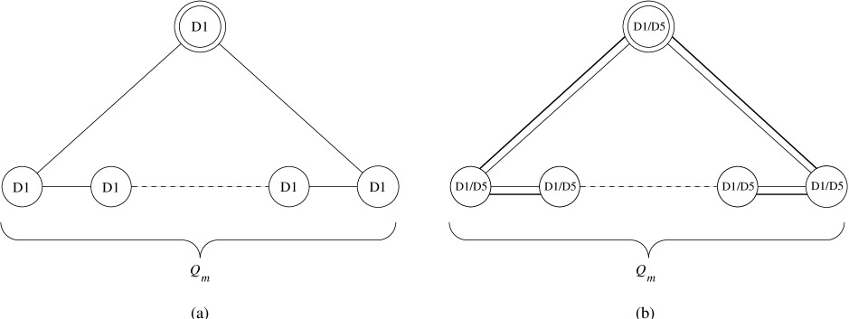
Figure 1: The extended Dynkin diagrams encoding the arrangement of open strings when (a) $Q_{1}$ D–strings and (b) $Q_{1}$ D–strings and $Q_{5}$ D5–branes are placed at an $A_{Q_{m}}$ singularity. The heavy lines are $(5,5)$ strings and the lighter lines are $(1,1)$ strings. Each circle represents one factor of (a) $U(Q_{1})$ or (b) $U(Q_{1})\times U(Q_{5})$. The double circle corresponds to the trivial representation.

Finally we come to the $(1,5)$ strings. The answer is found by combining the analyses of the previous paragraphs. Before performing the orbifold projection these strings are in the bi–fundamental representation of $U(Q_{m}Q_{1})\times U(Q_{m}Q_{5})$. As shown before the oscillators for these states are acted on trivially by $\mathbb{Z}_{Q_{m}}$ thus the constraint is simply a generalization of that presented in eqn. (17). The Chan–Paton factors of these states are now $Q_{m}Q_{1}\times Q_{m}Q_{5}$ matrices $\Omega$ which can be thought of as $Q_{m}\times Q_{m}$ matrices whose entries are $Q_{1}\times Q_{5}$ blocks. Following eqn. (17) we impose the constraint,

$$\tilde{\Omega}_{aB}=(\gamma_{Q_{1}})_{ac}\Omega_{cD}(\gamma_{Q_{5}})^{-1}_{DB}=\Omega_{aB}$$ (18)

where $\gamma_{Q_{1}}$ is as before, $\gamma_{Q_{5}}$ is formed by tensoring the $Q_{m}$ dimensional regular representation of $\mathbb{Z}_{Q_{m}}$ with the $Q_{5}\times Q_{5}$ identity matrix. Here lower case indices run over $1,\cdots,Q_{1}$ while upper case indices run over $1,\cdots,Q_{5}$. This constraint can only be solved by “diagonal” matrices whose entries are $Q_{1}\times Q_{5}$ blocks. There are therefore no strings in bi–fundamental representations of different factors of the gauge group. More succinctly there are no $(1,5)$ strings in the links of the Dynkin diagram. Thus the only $(1,5)$ strings are those which connect D1–branes and D5–branes in the same sector of the gauge theory. So our conclusion is that there are precisely $Q_{m}$ hyper-multiplets, one for each factor appearing in the gauge group, corresponding to $(1,5)$ and $(5,1)$ strings. See figure 1b.

Note that the low energy effective field theory discussed here will flow to a 1+1 dimensional conformal field theory in the IR which is dual to the near horizon geometry (12) discussed in section (2) — see refs. [43, 44]. We also refer to the reader to ref. [51] for a discussion of the closely related gauge theory appearing in the bound state of two D3–branes on an ALE singularity.

Now to give a microscopic account of the black hole entropy, we calculate the ground state degeneracy when $N$ units of momentum are introduced in the 1+1 dimensional gauge theory. There are a total of $Q_{m}$ hyper-multiplets coming from $(1,5)$ strings, each of which has $4Q_{1}Q_{5}$ boson/fermion ground states making a total of $4Q_{m}Q_{1}Q_{5}$. The degeneracy of states then comes from the number of ways we can distribute $N$ units of momentum to these degrees of freedom. Since this system is BPS, we can easily write the partition function for the momentum $N$ among these bosonic and fermionic states in the 1+1 dimensional effective theory as a purely chiral system:

$$\prod_{N=1}^{\infty}\left({1+q^{N}\over 1-q^{N}}\right)^{4Q_{m}Q_{1}Q_{5}}=\sum_{N=1}^{\infty}\Omega(N)q^{N}\ ,$$ (19)

where, at large $N$, the level degeneracy behaves as $\Omega(N)\sim\exp(2\pi\sqrt{Q_{m}Q_{1}Q_{5}N}).$ We see that the entropy is therefore

$$S=\log\Omega(N)=2\pi\sqrt{Q_{m}Q_{1}Q_{5}N}$$ (20)

which is precisely that given in eqn. (11)!

4 Discussion

So we have our desired result: The entropy of the four dimensional extremal black hole constructed from D1–branes, D5–branes, momentum and a Kaluza–Klein monopole, is indeed the product of four charges (associated to each sector) appropriate for the quartic invariant of $E_{(7)7}$. This has of course been shown elsewhere [9] using a different construction in the type IIA theory, not involving Kaluza–Klein monopoles, but related to the one presented here by U–duality. It is however, quite satisfying to show it explicitly with the original arrangement of constituents, and pleasing that the interpretation in terms of fractional branes involving the machinery of D–branes on ALE spaces manifests itself so clearly. In particular, the absence of $(1,5)$ strings stretching between different factors of the gauge group is quite dramatic, since had it been the naive result, the entropy would have acquired a factor of $Q_{m}$, instead of the required $Q_{m}^{1/2}$, which is a significant difference at large $Q_{m}$.

Note that the expression (20) cannot be the full U–duality invariant expression for the counting of the BPS states in this system. In particular, one might note that our result is not valid for small $N$. In general, we might expect corrections to appear for small values of the charges both in the gauge theory calculations and in the black hole entropy. The latter can arise from higher curvature corrections to the supergravity action, which will modify the form of the black hole solution (and hence its horizon area), and also introduce corrections to the Bekenstein-Hawking entropy formula [52] — for a general review, see ref. [53]. In certain cases, such subleading corrections to the entropy have been matched in microscopic string calculations for black holes with ${\cal N}=2$ supersymmetry [54, 55, 56]. Generically, one also finds logarithmic corrections [57] to black hole entropy in going beyond the large charge approximation used, e.g., in deriving eqn. (20) from the previous expression (19). It would be interesting to extend our calculations to determine the full U–duality invariant result using techniques analogous to those used in refs. [58].

Given the success of those techniques above in examining the D1–D5 bound state, it seems that the methods used here are likely to be useful in extending these results to a U–dual counting formula of the BPS states underlying the present four dimensional black holes. However, one should note that the most general supersymmetric configuration in four dimensions actually depends on five charges[59, 60]. That is while four charges is the minimum required to produce a non-vanishing value for the quartic invariant of $E_{(7)7}$, the generating solution from which one can obtain all other configurations by the action of U–duality actually carries five independent charges. Recently progress has been made in producing a microscopic description of the black hole entropy of such five charge configurations [61] by applying the approach of ref. [54] to an M-theory embedding of the solution. The simplest approach to adding a fifth charge to the present type IIB black holes would require introducing an additional momentum in the $x^{4}$ direction, as well as a diagonal wrapping of either the D1– or D5–branes on this direction. Certainly extending the present analysis to this more elaborate configuration would be a necessary first step in producing a complete U–duality invariant expression for the black hole entropy.

5 Acknowledgments

Research by RCM and NRC was supported by NSERC of Canada and Fonds FCAR du Québec. RCM and CVJ would like to thank the Aspen Center for Physics for hospitality during part of this work. We would also like to thank Øyvind Tafjord for useful conversations.

References

- [1] A. Strominger and C. Vafa, Phys. Lett. B379 (1996) 99 [hep-th/9601029].
- [2] J. Polchinski, Phys. Rev. Lett. 75 (1995) 4724, [hep-th/9510017].
- [3] S.W. Hawking, Commum. Math. Phys. 43 (1975) 1999; J.D. Bekenstein, Phys. Rev. D7 (1973) 2333; D9 (1974) 3292.
- [4] C.G. Callan and J.M. Maldacena, Nucl. Phys. B472 (1996) 591 [hep-th/9602043].
- [5] G.T. Horowitz and A. Strominger, Phys. Rev. Lett. 77 (1996) 2368 [hep-th/9602051].
- [6] J.C. Breckenridge, R.C. Myers, A.W. Peet and C. Vafa, Phys. Lett. B381 (1996) 93 [hep-th/9602065].
- [7] J.C. Breckenridge, D.A. Lowe, R.C. Myers, A.W. Peet, A. Strominger and C. Vafa, Phys. Lett. B381 (1996) 423 [hep-th/9603078].
- [8] C.V. Johnson, R.R. Khuri and R.C. Myers, Phys. Lett. B378 (1996) 78 [hep-th/9603061]
- [9] J.M. Maldacena and A. Strominger, Phys. Rev. Lett. 77 (1996) 428 [hep-th/9603060].
- [10] G.T. Horowitz, D.A. Lowe and J.M. Maldacena, Phys. Rev. Lett. 77 (1996) 430 [hep-th/9603195].
- [11] J.M. Maldacena, Ph.D. Thesis, Princeton University, [hep-th/9607235]
- [12] A.W. Peet, Class. Quant. Grav. 15 (1998) 3291 [hep-th/9712253].
- [13] D. Youm, Phys. Rept. 316 (1999) 1 [hep-th/9710046].
- [14] V. Balasubramanian, Cargese Lectures [hep-th/9712215]
- [15] S. Ferrara and R. Kallosh, Phys.Rev. D54 (1996) 1525 [hep-th/9602136]; J. Polchinski, unpublished
- [16] E. Cremmer and B. Julia, Nucl. Phys. B159 (1979) 141.
- [17] C.M. Hull and P.K. Townsend, Nucl. Phys. B438 (1995) 109 [hep-th/9410167].
- [18] R. Kallosh and B. Kol, Phys. Rev. D53 (1996) 5344 [hep-th/9602014].
- [19] V. Balasubramanian and F. Larsen, Nucl. Phys. B478 (1996) 199 [hep-th/9604189].
- [20] S. Ferrara and J. Maldacena, Class. Quant. Grav. 15 (1998) 749 [hep-th/9706097].
- [21] R. Kallosh, A. Linde, T. Ortin, A. Peet and A. Van Proeyen, Phys. Rev. D46, 5278 (1992) [hep-th/9205027].
- [22] M. J. Duff, R. R. Khuri, R. Minasian and J. Rahmfeld, Nucl. Phys. B418, 195 (1994) [hep-th/9311120].
- [23] M. J. Duff and J. Rahmfeld, Phys. Lett. B345, 441 (1995) [hep-th/9406105].
- [24] R. R. Khuri and T. Ortin, Nucl. Phys. B467, 355 (1996) [hep-th/9512177]; Phys. Lett. B373, 56 (1996) [hep-th/9512178].
- [25] M. Cvetic and D. Youm, Nucl. Phys. B453, 259 (1995) [hep-th/9505045]; Phys. Rev. D53, 584 (1996) [hep-th/9507090]; Phys. Rev. Lett. 75, 4165 (1995) [hep-th/9503082]; Phys. Lett. B359, 87 (1995) [hep-th/9507160].
- [26] M. Cvetic and A. Tseytlin, Phys. Lett. B366, 95 (1996) [hep-th/9510097].
- [27] H. Lu and C. N. Pope, Nucl. Phys. B465, 127 (1996) [hep-th/9512012]; Int. J. Mod. Phys. A12, 437 (1997) [hep-th/9512153].
- [28] D.J. Gross and M.J. Perry, Nucl. Phys. B226 (1983) 29; R.D. Sorkin, Phys. Rev. Lett. 51 (1983) 87.
- [29] S.W. Hawking, Phys. Lett. 60A (1977) 81.
- [30] G.W. Gibbons and S.W. Hawking, Phys. Lett. B78 (1978) 430.
- [31] M.R. Douglas and G. Moore, Dbranes, Quivers and ALE Instantons [hep-th/9603167]
- [32] C.V. Johnson and R.C. Myers, Phys. Rev. D55 (1997) 6382 [hep-th/9610140].
- [33] E. Gimon and J. Polchinski, Phys. Rev. D54 (1996) 1667 [hep-th/9601038].
- [34] E. Gimon and C.V. Johnson, Nucl. Phys. B477 (1996) 715 [hep-th/9604129].
- [35] A. Dabholkar and J. Park, Nucl. Phys. B472 (1996) 207 [hep-th/9602030].
- [36] D. Diaconescu, M.R. Douglas and J. Gomis, JHEP 9802 (1998) 13 [hep-th/9712230].
- [37] A.H. Taub, Ann. Math. 53 (1951) 472; E. Newmann, L. Tamburino and T. Unti, J. Math. Phys.4 (1963) 915.
- [38] A.A. Tseytlin, Nucl. Phys. B475 (1996) 149 [hep-th/9604035]; J.P. Gauntlett, D.A. Kastor and J. Traschen, Nucl. Phys. B478 (1996) 544 [hep-th/9604179].
- [39] J. Maldacena, Adv. Theor. Math. Phys. 2 (1998) 231 [hep-th/9711200].
- [40] O. Aharony, S. S. Gubser, J. Maldacena, H. Ooguri and Y. Oz, Phys. Rept. 323, 183 (2000) [hep-th/9905111].
- [41] J. Maldacena and A. Strominger, JHEP 9812 (1998) 005 [hep-th/9804085].
- [42] S. Kachru and E. Silverstein, Phys. Rev. Lett. 80 (1998) 4855 [hep-th/9802183].
- [43] K. Behrndt, I. Brunner and I. Gaida, Nucl. Phys. B546 (1999) 65 [hep-th/9806195].
- [44] Y. Sugawara, JHEP 9906 (1999) 35 [hep-th/9903120].
- [45] D. Kutasov, F. Larsen and R. G. Leigh, Nucl. Phys. B550 (1999) 183 [hep-th/9812027].
- [46] E. Witten, Nucl. Phys. B460 (1996) 541 [hep-th/9511030].
- [47] J. Polchinski, Phys. Rev. D55, 6423 (1997) [hep-th/9606165].
- [48] C.V. Johnson, “D–Brane Primer”, [hep-th/0007170].
- [49] J. Polchinski, “TASI Lectures on D–branes”, [hep-th/9611050].
- [50] See for example: J.P. Elliot and P.G. Dawber, Symmetry in Physics, McMillan, 1986.
- [51] D. Berenstein and R. G. Leigh, Phys. Rev. D60 (1999) 026005 [hep-th/9812142].
- [52] R.M. Wald, Phys. Rev. D48 (1993) 3427 [gr-qc/9307038]; V. Iyer and R.M. Wald, Phys. Rev. D50 (1994) 846 [gr-qc/9403028]; T. Jacobson and R.C. Myers, Phys. Rev. Lett. 70 (1993) 3684 [hep-th/9305016]; T. Jacobson, G. Kang and R.C. Myers, Phys. Rev. D49 (1994) 6587 [gr-qc/9312023]; Phys. Rev. D52 (1995) 3518 [gr-qc/9503020].
- [53] R. C. Myers, “Black holes in higher curvature gravity,” gr-qc/9811042.
- [54] J. Maldacena, A. Strominger and E. Witten, JHEP 9712 (1997) 2 [hep-th/9711053].
- [55] C. Vafa, Adv. Theor. Math. Phys. 2 (1998) 207 [hep-th/9711067].
- [56] K. Behrndt, G. Lopes Cardoso, B. de Wit, D. Lust, T. Mohaupt and W.A. Sabra, Phys. Lett. B429 (1998) 289 [hep-th/9801081]; G. Lopes Cardoso, B. de Wit and T. Mohaupt, Phys. Lett. B451 (1999) 309 [hep-th/9812082]; Fortsch. Phys. 48 (2000) 49 [hep-th/9904005]; Nucl. Phys. B567 (2000) 87 [hep-th/9906094]; Class. Quant. Grav. 17 (2000) 1007 [hep-th/9910179].
- [57] S. Carlip, “Logarithmic corrections to black hole entropy from the Cardy formula,” gr-qc/0005017; D. Birmingham and S. Sen, “An exact black hole entropy bound,” hep-th/0008051.
- [58] R. Dijkgraaf, G. Moore, E. Verlinde and H. Verlinde, Commun. Math. Phys. 185 (1997) 197 [hep-th/9608096]; J. Maldacena, G. Moore and A. Strominger, “Counting BPS black holes in toroidal type II string theory,” [hep-th/9903163]; R. Dijkgraaf, J. Maldacena, G. Moore and E. Verlinde, “A black hole farey tail,” hep-th/0005003.
- [59] M. Cvetic and C. M. Hull, Nucl. Phys. B480 (1996) 296 [hep-th/9606193]; M. Cvetic and D. Youm, Nucl. Phys. B472 (1996) 249 [hep-th/9512127]; M. Cvetic and A. A. Tseytlin, Phys. Rev. D53 (1996) 5619 [hep-th/9512031]; Erratum – ibid. D55 (1997) 3907.
- [60] M. Bertolini, P. Frè and M. Trigiante, Class. Quant. Grav. 16 (1999) 2987 [hep-th/9905143].
- [61] M. Bertolini and M. Trigiante, “Microscopic entropy of the most general four-dimensional BPS black hole,” [hep-th/0008201]; Nucl. Phys. B582 (2000) 393 [hep-th/0002191]; “Regular R-R and NS-NS BPS black holes,” hep-th/9910237.