$\ast$-Trek:
The One-Loop ${\mathcal{N}}=4$ Noncommutative SYM Action

Abstract:

We investigate ${\mathcal{N}}=4$ noncommutative super Yang-Mills (SYM) theory. We compute the one-loop four gauge boson scattering amplitude on parallel D$p$-branes, and find the corresponding contribution to the noncommutative SYM one-loop action in a momentum expansion. The result is somewhat surprising. We find that while the planar diagram can be written using the usual $\ast$-product, the contributions from nonplanar diagrams in general involve additional structure beyond the $\ast$-product, arising from the nontrivial worldsheet correlations surviving the field theory limit. To each nonplanar diagram, depending on the number $n$ of external vertex operator insertions on each boundary, there is a corresponding $\ast_{n}$ $n$-ary operation. We further find that it is no longer possible to write down an off-shell gauge invariant one-loop effective action using the noncommutative field strength defined at tree-level.

1 Introduction

Field and string theories on noncommutative space(time) have attracted much attention recently [1, 2]. They appear naturally in various decoupling limits of the worldvolume theories of D-branes in a background NS-NS $B$-field [3, 4, 5, 6, 7, 8]. While much progress has been made in understanding the perturbative dynamics [9, 10, 11, 12] and their strong coupling limits [4, 5, 13, 6, 8], many fundamental issues remain obscure.

In noncommutative gauge theories, gauge invariance becomes much more subtle. The gauge group and the allowed representations of the gauge group are highly constrained. A basic example is that in noncommutative field theory, $SO(2)$ is not a good gauge group even though the isomorphic $U(1)$ is. The first statement follows from the fact that

$$\left(\begin{smallmatrix}0&f(x)\\ -f(x)&0\end{smallmatrix}\right)\ast\left(\begin{smallmatrix}0&g(x)\\ -g(x)&0\end{smallmatrix}\right)-\left(\begin{smallmatrix}0&g(x)\\ -g(x)&0\end{smallmatrix}\right)\ast\left(\begin{smallmatrix}0&f(x)\\ -f(x)&0\end{smallmatrix}\right)\\ =\left(\begin{smallmatrix}-f(x)\ast g(x)+g(x)\ast f(x)&0\\ 0&-f(x)\ast g(x)+g(x)\ast f(x)\end{smallmatrix}\right),$$ (1)

which is not an element of the $SO(2)$ algebra. It is also interesting that, in theories with only adjoint matter, translations along noncommutative directions are a subset of gauge transformations, and thus there are no gauge invariant local operators [14, 15].

Another puzzling issue is the contributions of the nonplanar diagrams to the 1PI effective action of the noncommutative field theories. One generically encounters IR singularities when an external momentum crosses an internal line in a nonplanar diagram for which the internal momentum integration is UV divergent at $\Theta=0$; this is the so-called IR/UV mixing. The presence of IR/UV mixing indicates that the long distance behaviour of the system is no longer insensitive to the short distance physics, and the UV cutoff might not be pushed to infinity in a consistent way (see, however, [17]).

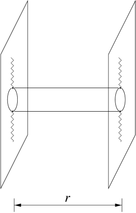
Figure 1: An example of the scattering amplitude considered. This is the nonplanar diagram with two gluons on each brane (a $2\rightarrow 2$ process).

In [18], it was suggested that IR/UV mixing may be naturally understood in terms of a “stretched string”. When $B\neq 0$, an open string has a nonzero stretched displacement $\Delta x=\Theta k$, even in the field theory limit ${{\alpha^{\prime}}}\rightarrow 0$. As the momentum $k$ is increased, the string stretches longer. Thus when there is a net momentum flow $k$ between the two ends of the open string, as in the case of a nonplanar diagram, the integrated loop particle has to propagate an additional distance $\left\lvert{\Delta x}\right\rvert$, the effect of which is to seemingly cut open an otherwise closed first-quantized particle loop. When, for $B=0$, the loop integral is divergent at short distances, the stretched string acts as an effective short-distance cutoff and regularizes the divergence. However, since taking $\Delta x$ to zero (IR for external momentum $k$) will recover the original UV divergence, the amplitude is generally singular as $\Delta x\rightarrow 0$. Thus, $k\rightarrow 0$ is not a continuous limit, and the singularity at small $k$ reflects the UV divergence of the $B=0$ theory. The stretched string can also be used to understand two-loop computations.[22]

In this paper we further explore the IR/UV effects of the stretched string. To keep the IR singularities from obscuring our understanding, we consider a highly supersymmetric example: ${\mathcal{N}}=4$ noncommutative SYM theory. Since this theory is finite in the commutative limit, the nonplanar diagrams are not plagued by the IR singularities mentioned above. We are thus able to give an explicit and unambiguous result for its one-loop scattering amplitudes. Various issues, including the contributions from nonplanar diagrams and one-loop off-shell gauge invariance can then be discussed in a controlled manner.

Like the commutative theory, there is no 1-loop contribution to the two and three-point amplitudes in ${\mathcal{N}}=4$ noncommutative SYM theory. We will thus focus on the four-point amplitudes, specifically the four gauge boson annulus amplitude (e.g. figure 1). The leading order contribution in the low energy limit determines the $F^{4}$ term in the low energy effective action of noncommutative ${\mathcal{N}}=4$ super-Yang-Mills theory. Since we are interested in exploring the effect of noncommutativity, we take the low energy limit to mean

$$\frac{k_{i}G^{-1}k_{j}}{m^{2}}\ll 1\qquad\text{with}\qquad k_{i}\Theta k_{j}\sim{{\mathcal{O}}({1})},$$ (2)

for external momenta $k_{i}$, where $m$ is the mass of the W-bosons stretched between the branes.

Before we begin, let us recall the commutative result. For convenience, we restrict ourselves to the case of two single branes. To lowest order in external momenta, the one-loop amplitude for four gauge bosons can be written in the form (see e.g. [23, 24])

$$\Gamma_{\rm{1-loop}}\propto\frac{1}{r^{4}}\int d^{4}y\bigl{[}F^{\mu}{{}_{\nu}}F^{\nu}{{}_{\rho}}F^{\rho}{{}_{\kappa}}F^{\kappa}{{}_{\mu}}-\frac{1}{4}F^{\mu}{{}_{\nu}}F^{\nu}{{}_{\mu}}F^{\rho}{{}_{\kappa}}F^{\kappa}{{}_{\rho}}\bigr{]}.$$ (3)

where $F=F_{1}-F_{2}$ and the subscripts $1,2$ refer to the two D3-branes.

The factor of $\frac{1}{r^{4}}$ in equations (3) arises in the SYM box diagram via the $W$-boson mass [$m=\frac{r}{2\pi{{\alpha^{\prime}}}}$] in the propagators. Alternatively, one can understand it as arising via the propagator for exchange of massless closed strings in the transverse space between the branes.

When we turn on a nonvanishing $\Theta$, we find some new interesting phenomena for the nonplanar amplitudes:

• Due to the extra propagating distance $\left\lvert{\Delta x}\right\rvert=|\Theta k|$ for the W-bosons running in the loop, where $k$ now is the momentum flow between the branes, the factor $\frac{1}{r^{4}}$ is replaced by

  $$\frac{1}{m^{4}}K_{2}(m\left\lvert{\Delta x}\right\rvert),\qquad m=\frac{r}{2\pi{{\alpha^{\prime}}}}.$$ (4)

  where $K_{2}$ is a modified Bessel function. In particular, when $m\left\lvert{\Delta x}\right\rvert\gg 1$, the amplitude is exponentially suppressed, proportional to

  $$\exp[-m\left\lvert{\Delta x}\right\rvert]$$ (5)

  typical of an intermediate particle of mass $m$ propagating over a distance $\left\lvert{\Delta x}\right\rvert$. From the closed string point of view, equation (4) implies that the closed strings propagating between the branes are massive. Due to different scalings between the closed and open string metrics, the low energy limit on the brane in terms of open string metric $G_{\mu\nu}$ no longer implies the low energy limit for the bulk closed string modes. Thus, in the kinematic regime (2), there is a significant longitudinal momentum transfer between the branes, and the closed string modes indeed obtain an effective mass $M=\frac{\left\lvert{\Delta x}\right\rvert}{2\pi{{\alpha^{\prime}}}}=\frac{|\Theta k|}{2\pi{{\alpha^{\prime}}}}$.

• We have attempted to write down a one-loop effective action, from integrating out massive W-bosons, in terms of a derivative expansion in the regime (2). We find that while it is possible to formally write down an off-shell effective action from the gauge invariant on-shell amplitudes, the off-shell action is not gauge invariant in terms of the noncommutative $F_{\mu\nu}$,

  $$F_{\mu\nu}=\partial_{\mu}A_{\nu}-\partial_{\nu}A_{\mu}-iA_{\mu}\ast A_{\nu}+iA_{\nu}\ast A_{\mu},$$ (6)

  defined at tree-level. The technical reason is the following. In nonplanar processes, writing an effective action requires additional $\ast$-operations which are not gauge invariant under the gauge transformations of the noncommutative $F$. For example, for the $2\rightarrow 2$ process of figure 1, the product between two photon modes on the same worldsheet boundary becomes

  $$F^{\mu\nu}\ast^{\prime}F_{\mu\nu},$$ (7)

  where the $\ast^{\prime}$-product is given by

  $$\begin{split}f(x)\ast^{\prime}g(x)&\equiv f(x)\frac{\sin\bigl{(}\frac{1}{2}\Theta^{\mu\nu}\overleftarrow{{\partial}_{\mu}}\overrightarrow{{\partial}_{\nu}}\bigr{)}}{\frac{1}{2}\Theta^{\mu\nu}\overleftarrow{{\partial}_{\mu}}\overrightarrow{{\partial}_{\nu}}}g(x),\\ &=f(x)g(x)-\frac{1}{24}\Theta^{\mu\nu}\Theta^{\sigma\tau}\partial_{\mu}\partial_{\sigma}f(x)\partial_{\nu}\partial_{\tau}g(x)+\ldots\ .\end{split}$$ (8)

  The result is somewhat surprising. From the field theory point of view, we have integrated out the massive $W$-bosons. According to conventional wisdom, we should be able to write down a gauge-invariant effective action as a derivative expansion. That it is no longer possible to do so might be another indication of IR/UV mixing in noncommutative theories, even though in this case we do not have the IR singularities.

The paper is organized as follows. In section 2, we evaluate the string amplitude. The field theory limit is explored in section 3. In section 4, we conclude with a discussion of gauge invariance. We describe our treatment of the fermionic string coordinates in the presence of a $B$-field, used in section 2, in appendix A.

2 Correlation Functions

We are interested in computing the one-loop scattering amplitudes of “brane waves” on parallel D$p$-branes in type II string theory—specifically, the four gauge boson annulus amplitude, both planar and nonplanar (e.g. figure 1).

On the annulus, we can work in the “zero” picture, for which the relevant vertex operator is [25]

$${\mathcal{V}}^{0}=\frac{g_{o}}{\sqrt{2{{\alpha^{\prime}}}}}T^{a}e_{\mu}^{a}(i\dot{X}^{\mu}+4k\cdot\Psi\Psi^{\mu})e^{ik\cdot X}.$$ (9)

In equation (9), $T^{a}$ is a generator of the gauge group, $e^{a}_{\mu}$ is the polarization of the gluon and $\Psi^{\mu}$ is the linear combination of the left and right-moving fermions, $\psi$ and $\tilde{\psi}$, that lives on the boundary (see appendix A). The dot product is simple contraction: $k\cdot\Psi\equiv k_{\mu}\Psi^{\mu}$. For general periodicity $\psi^{\mu}(w+2n\pi+2m\pi it)=e^{2\pi i[n(\alpha-1/2)+m(\beta-1/2)]}\psi^{\mu}(w)$, the Green functions for $\Psi$ can be written

$${\left\langle{\Psi^{\mu}(w_{1})\Psi^{\nu}(w_{2})}\right\rangle}=\frac{{{\alpha^{\prime}}}}{4\pi}G^{\mu\nu}\frac{\vartheta\left[\begin{smallmatrix}\alpha\\ \beta\end{smallmatrix}\right]\bigl{(}\frac{w_{1}-w_{2}}{2\pi}|it\bigr{)}\vartheta^{\prime}\left[\begin{smallmatrix}1/2\\ 1/2\end{smallmatrix}\right](0|it)}{\vartheta\left[\begin{smallmatrix}1/2\\ 1/2\end{smallmatrix}\right]\bigl{(}\frac{w_{1}-w_{2}}{2\pi}|it\bigr{)}\vartheta\left[\begin{smallmatrix}\alpha\\ \beta\end{smallmatrix}\right](0|it)}, {}^{\prime}{{}^{\prime}}$$ (57)

and the partition function is

$${\left\langle{1}\right\rangle}=\frac{\vartheta\left[\begin{smallmatrix}\alpha\\ \beta\end{smallmatrix}\right]\bigl{(}0|it\bigr{)}^{4}}{\eta(it)^{4}}.$$ (56^′)

It is well known (see e.g. [25]) that, on the annulus, the first nonvanishing correlation function involves four pairs of fermions. This gives the one-loop nonrenormalization theorem for the $F^{2}$ and $F^{3}$ terms in the effective supersymmetric spacetime action. Because the effect of the $B$-field on the fermions can be absorbed into the doubling trick, this continues to hold. Thus, the first nontrivial amplitude on the annulus involves four gauge bosons, and the corresponding amplitude is

$$\sum_{\pm,\pm^{\prime}}\frac{g_{o}^{4}}{4{{\alpha^{\prime}}}^{2}}\,(2\alpha^{\prime})^{4}\,T^{a}T^{b}T^{c}T^{d}e^{a}_{1\mu}e^{b}_{2\nu}e^{c}_{3\rho}e^{d}_{4\sigma}{\left\langle{e^{ik_{1}\cdot X}(w_{1})e^{ik_{2}\cdot X}(w_{2})e^{ik_{3}\cdot X}(w_{3})e^{ik_{4}\cdot X}(w_{4})}\right\rangle}\\ \times{\left\langle{{{:}{k_{1}{\cdot}\Psi\Psi^{\mu}}{:}}(w_{1})\;{{:}{k_{2}{\cdot}\Psi\Psi^{\nu}}{:}}(w_{2})\;{{:}{k_{3}{\cdot}\Psi\Psi^{\rho}}{:}}(w_{3})\;{{:}{k_{4}{\cdot}\Psi\Psi^{\sigma}}{:}}(w_{4})}\right\rangle}_{\pm\pm^{\prime}}$$ (10)

where we have factored the amplitude into fermionic and bosonic factors, and suppressed the ghosts. The sum is over spin structures. The fermionic contribution is easily found to be

$$\sum_{\pm,\pm^{\prime}}{\left\langle{{{:}{k_{1}{\cdot}\Psi\Psi^{\mu}}{:}}(w_{1})\;{{:}{k_{2}{\cdot}\Psi\Psi^{\nu}}{:}}(w_{2})\;{{:}{k_{3}{\cdot}\Psi\Psi^{\rho}}{:}}(w_{3})\;{{:}{k_{4}{\cdot}\Psi\Psi^{\sigma}}{:}}(w_{4})}\right\rangle}_{\pm\pm^{\prime}}\\ =\eta(it)^{8}k_{1\tau}k_{2\lambda}k_{3\alpha}k_{4\beta}\,t^{\tau\mu\lambda\nu\alpha\rho\beta\sigma},$$ (11)

where $t^{\alpha_{1}\beta_{1}\alpha_{2}\beta_{2}\alpha_{3}\beta_{3}\alpha_{4}\beta_{4}}$ is antisymmetric in $\alpha_{i}\leftrightarrow\beta_{i}$ (for each $i$) and is symmetric in $(\alpha_{i},\beta_{i})\leftrightarrow(\alpha_{j},\beta_{j})$. It is convenient to define

$${\mathcal{K}} \equiv k_{1\alpha_{1}}e^{a}_{1\beta_{1}}k_{2\alpha_{2}}e^{b}_{2\beta_{2}}k_{3\alpha_{3}}e^{c}_{3\beta_{3}}k_{4\alpha_{4}}e^{d}_{4\beta_{4}}t^{\alpha_{1}\beta_{1}\alpha_{2}\beta_{2}\alpha_{3}\beta_{3}\alpha_{4}\beta_{4}}$$ (12a)

which gives

$${\mathcal{K}} =M_{1\mu}{{}^{\lambda}}M_{2\lambda}{{}^{\alpha}}M_{3\alpha}{{}^{\nu}}M_{4\nu}{{}^{\mu}}-\frac{1}{4}M_{1\mu\nu}M_{2}^{\nu\mu}M_{3\tau\sigma}M_{4}^{\sigma\tau}+\text{2 permutations}.$$ (12b)

In (12), $M_{i\mu\nu}=e_{i\mu}k_{i\nu}-k_{i\mu}e_{i\nu}$, the indices are raised and lowered using the open string metric $G$, and the two permutations are given by changing the ordering from (1234) to $(1342)$ and $(1423)$ (see e.g. [25]).

The bosonic contribution is identical to the tachyon correlation function computed for the bosonic string in [27, 28, 29, 30, 18, 31]. Combining equations (11) and [18, eq. (2.15)] gives the total amplitude

$${\mathcal{A}}=-i\sqrt{\det G}\frac{g_{o}^{4}}{4{{\alpha^{\prime}}}^{2}}(2{{\alpha^{\prime}}})^{4}\,(2\pi)^{p+1}\delta^{(p+1)}\Bigl{(}\text{\small$\sum_{q=1}^{4}$}k_{q}\Bigr{)}\,{\mathcal{K}}\\ \times\int_{0}^{\infty}\frac{dt}{2t}(8\pi^{2}{{\alpha^{\prime}}}t)^{-\frac{p+1}{2}}\,\exp\left[\frac{k_{\mu}(\Theta G\Theta)^{\mu\nu}k_{\nu}}{8\pi{{\alpha^{\prime}}}t}-\frac{r^{2}t}{2\pi{{\alpha^{\prime}}}}\right]\left[\prod_{q=1}^{4}\int_{0}^{2\pi t}d\tau_{q}\right]\,\Psi_{1}\Psi_{2}\Psi_{12}\\ \times\exp\left[-\frac{i}{2}\sum_{i<j}(k_{i}\times k_{j})[\frac{\tau_{ij}}{\pi t}-\epsilon(\tau_{ij})]+\frac{i}{2}\sum_{y<z}(k_{y}\times k_{z})[\frac{\tau_{yz}}{\pi t}-\epsilon(\tau_{yz})]\right]$$ (13)

where $\tau_{ij}=\tau_{i}-\tau_{j}$, $k=\sum_{i}k_{i}=-\sum_{y}k_{y}$ is the nonplanar momentum, $\epsilon(\tau)$ is the sign of $\tau$, and

$$\begin{aligned} \Psi_{1}&=\prod_{i<j}\left\lvert{\psi_{ij}}\right\rvert^{2{{\alpha^{\prime}}}k_{i\mu}G^{\mu\nu}k_{j\nu}},&\Psi_{2}&=\prod_{y<z}\left\lvert{\psi_{yz}}\right\rvert^{2{{\alpha^{\prime}}}k_{y\mu}G^{\mu\nu}k_{z\nu}},&\Psi_{12}&=\prod_{i,y}(\psi^{T}_{iy})^{2{{\alpha^{\prime}}}k_{y\mu}G^{\mu\nu}k_{i\nu}},\end{aligned}$$ (14a)

$$\begin{aligned} \psi_{ij}&=2\pi i\exp\left(-\frac{\tau_{ij}^{2}}{4\pi t}\right)\frac{\vartheta_{1}(i\frac{\tau_{ij}}{2\pi}|it)}{\vartheta_{1}^{\prime}(0|it)},&\psi_{iy}^{T}&=2\pi\exp\left(-\frac{\tau_{iy}^{2}}{4\pi t}\right)\,\frac{\vartheta_{2}(i\frac{\tau_{iy}}{2\pi}|it)}{\vartheta_{1}^{\prime}(0|it)}.\end{aligned}$$ (14b)

Here, $i$ and $y$ are indices which run over the vertex operators on the two boundaries, and $q$ runs over all vertex operators. The quantity ${\mathcal{K}}$ was given in (12), and we have suppressed Chan-Paton factors. We also have introduced a transverse distance $r$ between the parallel branes. It gives a mass

$$m=\frac{r}{2\pi{{\alpha^{\prime}}}}$$ (15)

to the ground states of open strings stretching between the branes and acts as an infrared cutoff in the world-volume Yang-Mills theory.

The exponential factor

$$\exp\left[\frac{1}{8\pi\alpha^{\prime}t}k_{\mu}(\Theta G\Theta)^{\mu\nu}k_{\nu}\right]=\exp\left[-\frac{(\Delta x)^{2}}{8\pi\alpha^{\prime}t}\right],\qquad\Delta x^{\mu}\equiv\Theta^{\mu\nu}k_{\nu},$$ (16)

in (13), which was interpreted in [18] as the manifestation of a stretched string in the bosonic string theory, and was responsible for IR/UV mixing in those theories, survives the field theory limit in the superstring as well. Thus, the observations made in [18] apply also here.

3 One-loop Amplitude in Noncommutative ${\mathcal{N}}=4$ SYM

The one-loop amplitude for noncommutative ${\mathcal{N}}=4$ super-Yang-Mills theory can be obtained from (13) by taking ${{\alpha^{\prime}}}\rightarrow 0$ with ${{\alpha^{\prime}}}t$ fixed. While our main focus is on the 3+1-dimensional ${\mathcal{N}}=4$ noncommutative SYM theory, our results apply to generic $p$, and we will keep our discussion general. To take the field theory limit, we have been implicitly considering only magnetic $B$; however, the results of section 2 are completely general, holding also for electric $B$, and so can be used in the context of the NCOS [4, 5, 6, 7, 8]. Note that as $t\rightarrow\infty$,

$$\psi_{ij} =-2\sinh\bigl{(}\frac{\tau_{ij}}{2}\bigr{)}\exp\bigl{(}-\frac{\tau_{ij}^{2}}{4\pi t}\bigr{)}, \psi_{iy}^{T} =2\cosh\bigl{(}\frac{\tau_{iy}}{2}\bigr{)}\exp\bigl{(}-\frac{\tau_{iy}^{2}}{4\pi t}\bigr{)}.$$ (17)

To isolate the $t$ dependence we rescale $\tau$ so that $0<\tau<1$. Let $T=2\pi m^{2}{{\alpha^{\prime}}}t$ and recall that $g_{\text{YM}}=g_{o}/\sqrt{2{{\alpha^{\prime}}}}$. This gives the field theory amplitude

$${\mathcal{A}}=-i2^{4}\pi^{\frac{p+1}{2}}\sqrt{\det G}g_{\text{YM}}^{4}\,\delta^{(p+1)}\Bigl{(}\text{\small$\sum_{q=1}^{4}$}k_{q}\Bigr{)}\,{\mathcal{K}}\,m^{p-7}\int_{0}^{\infty}\frac{dT}{2T}\,T^{\frac{7-p}{2}}\exp\left[-\frac{m^{2}(\Delta x)^{2}}{4T}-T\right]\\ \times\left[\prod_{q=1}^{4}\int_{0}^{1}d\tau_{q}\right]\exp\left[-\frac{i}{2}\sum_{i<j}(k_{i}\times k_{j})[2\tau_{ij}-\epsilon(\tau_{ij})]+\frac{i}{2}\sum_{y<z}(k_{y}\times k_{z})[2\tau_{yz}-\epsilon(\tau_{yz})]\right]\\ \times\exp\left[T\sum_{p<q}\frac{k_{p\mu}G^{\mu\nu}k_{q\nu}}{m^{2}}\bigl{[}\left\lvert{\tau_{pq}}\right\rvert-\tau_{pq}^{2}\bigr{]}\right].$$ (18)

Later we shall examine the amplitude (18) in the kinematic region $k_{p\mu}G^{\mu\nu}k_{q\nu}\ll m^{2}$, with $k_{p}\Theta k_{q}$ remaining finite [equation (2)]. In this case the last factor of (18) has the expansion

$$\left[1+T\sum_{p<q}\frac{k_{p\mu}G^{\mu\nu}k_{q\nu}}{m^{2}}\bigl{[}\left\lvert{\tau_{pq}}\right\rvert-\tau_{pq}^{2}\bigr{]}+\ldots\right].$$ (19)

Let us first look at the planar contribution. In this case $k=0$ and $\Delta x=0$. Also, $\sum_{i<j}(k_{i}\times k_{j})\tau_{ij}=0$ by momentum conservation; thus the phase factor in (18) is just

$$\exp\left[\frac{i}{2}\sum_{p<q}(k_{p}\times k_{q})\epsilon(\tau_{pq})\right].$$ (20)

This turns the amplitude

$${\mathcal{A}}\sim\frac{1}{m^{4}}\int d^{4}x\operatorname{Tr}F^{4}+\frac{1}{m^{2}}\int d^{4}x\operatorname{Tr}FFDFDF+\cdots$$ (21)

of the commutative theory into the

$${\mathcal{A}}\sim\frac{1}{m^{4}}\int d^{4}x\operatorname{Tr}(F\ast F\ast F\ast F)+\frac{1}{m^{2}}\int d^{4}x\operatorname{Tr}(F\ast F\ast DF\ast DF)+\cdots$$ (22)

of the noncommutative theory. (Here we have been schematic and have not included the Lorentz indices.)

The story for nonplanar diagrams is more complicated. There are essentially two new features for nonplanar diagrams in (18) compared to $B=0$ and the planar diagram. The first is the appearance, in the integral over proper time $T$, of $(\Delta x)^{2}$, in a manner which suppresses the contribution to the amplitude from small $T$ (short-distance). The second new feature is that in the integration of the vertex operator coordinates, there are additional phase factors

$$\exp\left[-i\sum_{i<j}(k_{i}\times k_{j})(\tau_{i}-\tau_{j})\right].$$ (23)

Both features already appeared in the bosonic cases [27, 29, 18]. Here with a large number of supersymmetries present, their effects can be isolated and subjected to a thorough analysis.

3.1 Stretched strings and closed strings

The factor $\exp\left[-\frac{m^{2}(\Delta x)^{2}}{4T}\right]$, in equation (18), was interpreted in [18] as the effect of a stretched string. More explicitly, when $B\neq 0$, an open string has a nonzero length, as described in the introduction, the effect of which is to cut open an otherwise closed first-quantized particle loop. The exponential factor may be understood as the amplitude for diffusion of a mass $m$ particle over a distance $\left\lvert{\Delta x}\right\rvert$. When, for $B=0$, the loop integral is divergent at short distances (small $T$), the stretched string effect regularizes the divergence. However, taking $\Delta x$ to zero will recover the original UV divergence. This is the origin of the IR/UV mixing discussed in [11]. In theories for which the commutative loop integral is convergent in the UV region, we would expect that the $\Delta x\rightarrow 0$ limit can be achieved in a continuous way, and that IR singularities are absent. It might be expected that the effect of the stretched string is mild in these cases. However, as we shall see below, it suppresses the amplitude exponentially at large external $k$.

In the low energy expansion in terms of $\frac{k_{p}\cdot k_{q}}{m^{2}}$ the integration over $T$ can be performed exactly for each term in the series and gives [32, eq. 8.432.6]

$$I_{n}=m^{p-7}\int_{0}^{\infty}\frac{dT}{2T}T^{\frac{7-p}{2}+n}e^{-\frac{m^{2}(\Delta x)^{2}}{4T}-T}=\left(\frac{m\left\lvert{\Delta x}\right\rvert}{2}\right)^{n}\left(\frac{2m}{\left\lvert{\Delta x}\right\rvert}\right)^{\frac{p-7}{2}}K_{\frac{7-p}{2}+n}(m\left\lvert{\Delta x}\right\rvert),$$ (24)

where $K$ is the modified Bessel function. Recall that $K_{-\nu}(z)=K_{\nu}(z)$ and as $z\rightarrow 0$,

$$K_{\nu}(z)=\begin{cases}\frac{\Gamma(\nu)}{2}\bigl{(}\frac{2}{z}\bigr{)}^{\nu},&\nu>0,\\ -\ln\frac{z}{2},&\nu=0.\end{cases}$$ (25)

For generic $p$ and $n$, as $\Delta x\rightarrow 0$, we have

$$I_{n}\sim\begin{cases}\frac{\Gamma\bigl{(}n+\frac{7-p}{2}\bigr{)}}{2}m^{p-7},&n+\frac{7-p}{2}>0,\\ -\log m\left\lvert{\Delta x}\right\rvert,&p=7,n=0,\\ \frac{\Gamma\bigl{(}\frac{7-p}{2}\bigr{)}}{2}(\frac{2}{\left\lvert{\Delta x}\right\rvert})^{p-7},&p=8,9;n=0,\\ -m^{2}\log(m\left\lvert{\Delta x}\right\rvert),&p=9,n=1.\end{cases}$$ (26)

When $n+\frac{7-p}{2}>0$, the integral in (24) is convergent as $\Delta x=0$; thus, as $\Delta x\rightarrow 0$, $I_{n}$ reduces to the standard results for $B=0$. In the other cases, logarithmic, linear and quadratic divergences, respectively for 8, 9 and 10-dimensional SYM theory, are reflected in the singular dependence on $\Delta x$ in the amplitude.

For $m\left\lvert{\Delta x}\right\rvert\gg 1$—i.e. the large external momentum limit—

$$I_{n}\sim\exp[-m\left\lvert{\Delta x}\right\rvert].$$ (27)

The amplitude is exponentially suppressed at large $k$. The behaviour in (27) is easily understood from the stretched string picture in which a particle of mass $m$ diffuses a distance $\left\lvert{\Delta x}\right\rvert$. This large momentum suppression is reminiscent of the asymptotic behaviour of correlation functions observed in the supergravity side [33] and the high temperature suppression of the partition function for nonplanar diagrams of ${\mathcal{N}}=4$ noncommutative SYM [34], although the details are somewhat different.

We note that for $n=0$—i.e. the leading term in the expansion (19)—there is also an interpretation for (24) in terms of the lowest closed string modes. Defining $M^{2}=(\frac{\Delta x}{2\pi{{\alpha^{\prime}}}})^{2}$ and $\tilde{d}=9-p$, the codimension of the brane, we can rewrite equation (24) as (notice that $Mr=m\left\lvert{\Delta x}\right\rvert$ )

$$I_{0}=(2\pi{{\alpha^{\prime}}})^{7-p}2\pi^{\frac{9-p}{2}}\int\frac{d^{\tilde{d}}q}{(2\pi)^{\tilde{d}}}\frac{e^{iq\cdot r}}{q^{2}+M^{2}}.$$ (28)

The right hand side of equation (28) has the interpretation of a massive particle of mass $M$ propagating between the branes. In contrast with the $B=0$ case ($\Delta x\rightarrow 0$ in (24)), for which the propagator is $m^{p-7}=\bigl{(}\frac{2\pi{{\alpha^{\prime}}}}{r}\bigr{)}^{7-p}$ corresponding to a virtual mediating massless closed string, now the propagating particle has a mass $M=\frac{\left\lvert{\Delta x}\right\rvert}{2\pi{{\alpha^{\prime}}}}$. This result can be understood by noting that the intermediate closed string has momentum $k_{\mu}$ (defined below equation (13)) along the brane direction from momentum conservation and therefore an effective mass

$$M^{2}=-k_{\mu}g^{\mu\nu}k_{\nu}=-k_{\mu}G^{\mu\nu}k_{\nu}+\left(\frac{1}{2\pi{{\alpha^{\prime}}}}\right)^{2}k_{\mu}(\Theta G\Theta)^{\mu\nu}k_{\nu}\sim\left(\frac{\Delta x}{2\pi{{\alpha^{\prime}}}}\right)^{2},$$ (29)

where in the last step we have recalled equation (2). Physically, this means that due to the different scaling between the closed and open string metrics, the low energy limit for the brane world-volume theory does not correspond to the low energy limit for the bulk closed string modes.

It is interesting to compare the IR/UV relation between the open and closed string pictures. For $p\leq 6$, SYM theory is IR divergent when $m=0$; this is reflected in the UV divergence, for codimension $\tilde{d}\geq 3$, of the transverse propagator on the closed string side, as we reduce the separation of the branes to zero. For $p=8,9$, the SYM theory is linearly and quadratically UV divergent while the transverse propagator is IR divergent ($M\rightarrow 0$) in codimension $\tilde{d}=1,0$. At $p=7$ SYM theory is both UV and IR divergent and the closed string propagator in codimension $2$ is both IR and UV divergent.

The UV/IR relations in equation (26) for $p=7,8,9$ are precise realizations of closed string idea proposed in [11, 12] to explain IR/UV mixing in noncommutative theories. However we note that that picture seems to apply only for the $n=0$ term, which is protected by a nonrenormalization theorem from contributions of massive string modes [35]. For higher order terms, in principle, there can be an infinite number of massive closed string modes involved. For example, the $p=9,n=1$ term is logarithmically divergent as $\Delta x\rightarrow 0$, but there is no propagation of a codimension two closed string to explain it.

3.2 Beyond the $\ast$-product

Now we would like to focus on the leading order ($n=0$) terms, and attempt to write down an off-shell gauge invariant one-loop effective action.

Due to the presence of the additional phase factors,

$$\exp\left[-i\sum_{i<j}(k_{i}\times k_{j})(\tau_{i}-\tau_{j})\right],$$ (30)

in the integrals over $\tau_{q}$ in (18), the product between the insertions on the same boundary is neither an ordinary nor a $\ast$-product, as it was for the $B=0$, and planar cases, respectively. In particular and interestingly, the nonplanar terms in the action are not $\ast$-product generalizations of the familiar ones.

For the nonplanar diagram with two vertex operators on each boundary (we label $1,2$ on one boundary and $3,4$ on the other), we find that the $\tau$-integrations give rise (including the Chan-Paton factors) to a factor of

$$\operatorname{Tr}(T^{a}T^{b})\operatorname{Tr}(T^{c}T^{d})\frac{\sin\bigl{(}\frac{k_{1}\times k_{2}}{2}\bigr{)}}{\frac{k_{1}\times k_{2}}{2}}\frac{\sin\bigl{(}\frac{k_{3}\times k_{4}}{2}\bigr{)}}{\frac{k_{3}\times k_{4}}{2}}.$$ (31)

Note that (31) is finite as $k_{1}\times k_{2}\rightarrow 0$ and/or $k_{3}\times k_{4}\rightarrow 0$.

The other type of nonplanar diagram has $1,2,3$ on one boundary and $4$ on the other. Then, for the ordering $\tau_{1}>\tau_{2}>\tau_{3}$,

$$\int_{0}^{1}d\tau_{1}\int_{0}^{\tau_{1}}d\tau_{2}\int_{0}^{\tau_{2}}d\tau_{3}\;e^{\frac{i}{2}(k_{1}\times k_{2}+k_{1}\times k_{3}+k_{2}\times k_{3})}e^{-i(k_{1}\times k_{2})\tau_{12}-i(k_{1}\times k_{3})\tau_{13}-i(k_{2}\times k_{3})\tau_{23}}\\ =\frac{e^{\frac{i}{2}(k_{1}\times k_{2}+k_{3}\times k_{4})}}{(k_{1}\times k_{4})(k_{3}\times k_{4})}+2\frac{e^{\frac{i}{2}k_{2}\times k_{3}}\sin\bigl{(}\frac{k_{1}\times k_{4}}{2}\bigr{)}}{(k_{1}\times k_{4})^{2}(k_{2}\times k_{4})}+2\frac{e^{\frac{i}{2}k_{1}\times k_{2}}\sin\bigl{(}\frac{k_{3}\times k_{4}}{2}\bigr{)}}{(k_{2}\times k_{4})(k_{3}\times k_{4})^{2}}.$$ (32)

This is nonsingular even when $k_{i}\times k_{j}\rightarrow 0$. Including all the orderings, as well as the minus sign that comes with the odd-number of Chan-Paton matrices on the $\sigma=\pi$ boundary, gives

$$-\operatorname{Tr}(T^{b}T^{a}T^{c})\operatorname{Tr}(T^{d})\left\{\frac{e^{\frac{i}{2}(k_{1}\times k_{2}+k_{1}\times k_{3}+k_{2}\times k_{3})}}{[k_{3}\times(k_{1}+k_{2})][k_{1}\times(k_{2}+k_{3})]}+\frac{e^{\frac{i}{2}(k_{2}\times k_{3}-k_{1}\times k_{2}-k_{1}\times k_{3})}}{[k_{1}\times(k_{2}+k_{3})][k_{2}\times(k_{1}+k_{3})]}\right.\\ \left.+\frac{e^{\frac{i}{2}(k_{1}\times k_{2}-k_{1}\times k_{3}-k_{2}\times k_{3})}}{[k_{2}\times(k_{1}+k_{3})][k_{3}\times(k_{1}+k_{2})]}\right\}\\ -\operatorname{Tr}(T^{a}T^{b}T^{c})\operatorname{Tr}(T^{d})\left\{\frac{e^{\frac{i}{2}(k_{2}\times k_{3}+k_{1}\times k_{3}-k_{1}\times k_{2})}}{[k_{3}\times(k_{1}+k_{2})][k_{2}\times(k_{1}+k_{3})]}+\frac{e^{\frac{i}{2}(k_{1}\times k_{3}+k_{1}\times k_{2}-k_{2}\times k_{3})}}{[k_{2}\times(k_{1}+k_{3})][k_{1}\times(k_{2}+k_{3})]}\right.\\ \left.+\frac{e^{-\frac{i}{2}(k_{1}\times k_{2}+k_{1}\times k_{3}+k_{2}\times k_{3})}}{[k_{1}\times(k_{2}+k_{3})][k_{3}\times(k_{1}+k_{2})]}\right\}.$$ (33)

When the gauge group is abelian, equation (33) can be simplified to

$$-\frac{\sin\bigl{(}\frac{k_{2}\times k_{3}}{2}\bigr{)}\sin\bigl{(}\frac{k_{1}\times(k_{2}+k_{3})}{2}\bigr{)}}{\frac{(k_{1}+k_{2})\times k_{3}}{2}\frac{k_{1}\times(k_{2}+k_{3})}{2}}-\frac{\sin\bigl{(}\frac{k_{1}\times k_{3}}{2}\bigr{)}\sin\bigl{(}\frac{k_{2}\times(k_{1}+k_{3})}{2}\bigr{)}}{\frac{(k_{1}+k_{2})\times k_{3}}{2}\frac{k_{2}\times(k_{1}+k_{3})}{2}}.$$ (34)

If we have $N$ vertex operators on the same boundary, the general product structure between the operators is given by

$$\operatorname{Tr}\left[T^{a_{1}}\dots T^{a_{N}}\right]\left[\prod_{q=1}^{N}\int_{0}^{\tau_{q-1}}d\tau_{q}\right]\exp\left[-\frac{i}{2}\sum_{i<j}(k_{i}\times k_{j})[2\tau_{ij}-\epsilon(\tau_{ij})]\right];\quad\tau_{0}\equiv 1,$$ (35)

plus permutations.

To lowest order in $k^{2}/m^{2}$, the four gluon scattering amplitudes are given by

$${\mathcal{A}}_{2\rightarrow 2}=-i2^{4}\pi^{\frac{p+1}{2}}\sqrt{\det G}g_{\text{YM}}^{4}\,\delta^{(p+1)}\Bigl{(}\text{\small$\sum_{q=1}^{4}$}k_{q}\Bigr{)}\,\operatorname{Tr}(T^{a}T^{b})\operatorname{Tr}(T^{c}T^{d})\;{\mathcal{K}}\,\\ \times\left(\frac{\Delta x}{2m}\right)^{\frac{7-p}{2}}K_{\frac{7-p}{2}}(m\Delta x)\,\frac{\sin\bigl{(}\frac{k_{1}\times k_{2}}{2}\bigr{)}}{\frac{k_{1}\times k_{2}}{2}}\frac{\sin\bigl{(}\frac{k_{3}\times k_{4}}{2}\bigr{)}}{\frac{k_{3}\times k_{4}}{2}},$$ (36)

where ${\mathcal{K}}$ is given by (12). Similarly (for simplicity, we only give the $U(1)$ result in this case),

$${\mathcal{A}}_{1\rightarrow 3}=i2^{4}\pi^{\frac{p+1}{2}}\sqrt{\det G}g_{\text{YM}}^{4}\,\delta^{(p+1)}\Bigl{(}\text{\small$\sum_{q=1}^{4}$}k_{q}\Bigr{)}\,{\mathcal{K}}\,\\ \times\left(\frac{\Delta x}{2m}\right)^{\frac{7-p}{2}}K_{\frac{7-p}{2}}(m\Delta x)\,\left[\frac{\sin\bigl{(}\frac{k_{2}\times k_{3}}{2}\bigr{)}\sin\bigl{(}\frac{k_{1}\times(k_{2}+k_{3})}{2}\bigr{)}}{\frac{(k_{1}+k_{2})\times k_{3}}{2}\frac{k_{1}\times(k_{2}+k_{3})}{2}}+\frac{\sin\bigl{(}\frac{k_{1}\times k_{3}}{2}\bigr{)}\sin\bigl{(}\frac{k_{2}\times(k_{1}+k_{3})}{2}\bigr{)}}{\frac{(k_{1}+k_{2})\times k_{3}}{2}\frac{k_{2}\times(k_{1}+k_{3})}{2}}\right].$$ (37)

It is easy to see that the above amplitudes are gauge invariant on-shell; i.e. ${\mathcal{A}}=0$, when we take $e_{i}\propto k_{i}$.

Now we would like to extend the above on-shell amplitudes to the off-shell effective action. The standard way of doing this is to take $M_{\mu\nu}=e_{\mu}k_{\nu}-e_{\nu}k_{\mu}\rightarrow-\frac{i}{g_{YM}}F_{\mu\nu}$ with $F_{\mu\nu}$ given by the tree-level expression

$$F_{\mu\nu}=\partial_{\mu}A_{\nu}-\partial_{\nu}A_{\mu}-iA_{\mu}\ast A_{\nu}+iA_{\nu}\ast A_{\mu}$$ (38)

Combining these expressions, we find that the 1-loop effective action contains the terms

$$\begin{split}\Gamma_{\text{1-loop}}&=-\frac{1}{4!(4\pi)^{\frac{p+1}{2}}}\int d^{p+1}x\,\sqrt{\det G}\,t^{\mu\nu\rho\sigma\lambda\tau\alpha\beta}\\ &\mspace{-40.0mu}\times\biggl{\{}\frac{N_{2}}{2}\Gamma\bigl{(}\frac{7-p}{2}\bigr{)}\frac{1}{m^{7-p}}\operatorname{Tr}_{U(N_{1})}[F_{\mu\nu}(x)\ast F_{\rho\sigma}(x)\ast F_{\lambda\tau}(x)\ast F_{\alpha\beta}(x)]\\ &\mspace{-40.0mu}+\left.3\operatorname{Tr}_{U(N_{1})}[F_{\mu\nu}(x)\ast^{\prime}F_{\rho\sigma}(x)]\,I_{\frac{7-p}{2}}\Bigl{(}m,\sqrt{\overleftarrow{{\partial}_{\mu}}\bigl{(}\Theta G\Theta\bigr{)}^{\mu\nu}\overrightarrow{{\partial}_{\nu}}}\Bigr{)}\operatorname{Tr}_{U(N_{2})}[F_{\lambda\tau}(x)\ast^{\prime}F_{\alpha\beta}(x)]\right.\\ &\mspace{-40.0mu}-\biggl{.}4\operatorname{Tr}_{U(N_{1})}\bigl{(}\ast_{3}[F_{\mu\nu}(x),F_{\rho\sigma}(x),F_{\lambda\tau}(x)]\bigr{)}I_{\frac{7-p}{2}}\Bigl{(}m,\sqrt{-\partial_{\mu}\bigl{(}\Theta G\Theta\bigr{)}^{\mu\nu}\partial_{\nu}}\Bigr{)}\operatorname{Tr}_{U(N_{2})}(F_{\alpha\beta}(x))\biggr{\}}\\ &\mspace{-40.0mu}+(N_{1}\rightarrow N_{2})\end{split}$$ (39a)

where $$N=N_{1}+N_{2} N_{1} N_{2} N_{1,2}$$ is the total number of D-branes with and D-branes on each boundary; the factor of appears in the planar diagram from tracing over the Chan-Paton factors on the empty boundary; the traces are taken in the fundamental of the indicated subgroup;

$$I_{n}(m,x)\equiv\left(\frac{x}{2m}\right)^{n}K_{n}(mx);$$ (39b)

and we have defined, from (31), the $\ast^{\prime}$-product (8), and from (33), the $\ast_{3}$-ternary operation. For an abelian gauge group, the $\ast^{\prime}_{3}$-ternary operation

$$\ast^{\prime}_{3}[f(x),g(x),h(x)]\\ \equiv\left[\frac{\sin\bigl{(}\frac{\partial_{2}\times\partial_{3}}{2}\bigr{)}\sin\bigl{(}\frac{\partial_{1}\times(\partial_{2}+\partial_{3})}{2}\bigr{)}}{\frac{(\partial_{1}+\partial_{2})\times\partial_{3}}{2}\frac{\partial_{1}\times(\partial_{2}+\partial_{3})}{2}}+\frac{\sin\bigl{(}\frac{\partial_{1}\times\partial_{3}}{2}\bigr{)}\sin\bigl{(}\frac{\partial_{2}\times(\partial_{1}+\partial_{3})}{2}\bigr{)}}{\frac{(\partial_{1}+\partial_{2})\times\partial_{3}}{2}\frac{\partial_{2}\times(\partial_{1}+\partial_{3})}{2}}\right]\left.{f(x_{1})g(x_{2})h(x_{3})}\right|_{x_{i}=x},$$ (40)

defined following (34), gives the same result as the similarly defined $\ast_{3}$-ternary operation. For the general product (35) we can define a $\ast_{n}$ $n$-ary operation which we will not write down explicitly.

We should note that (for $p<7$) equations (24) and (26) imply that the power expansion of $I_{\frac{7-p}{2}}(m,x)$ contains only nonnegative, even integer powers of $x$; thus equation (39a) contains only nonnegative integer powers of derivatives, and so is well-defined. The limit $\Theta\rightarrow 0$ is also well-defined—for example, all the $\ast_{n}$ $n$-ary operations become ordinary products—and recovers the nonabelian analogue of (3) given in e.g. [36] and references therein.

We have some remarks regarding equation (39):

• The $\ast^{\prime}$-product was also found by Garousi in [37]. When considering the scattering amplitudes of one closed string with two open string modes, he found that the $\ast^{\prime}$-product should be used to multiply the massless open string fields.

• The nonplanar part of equation (39) is not gauge-invariant, off-shell. To be specific, we focus on the second line of (39a); the symmetry of the expression—and particularly that of the $\ast^{\prime}$-product—implies that this term transforms into

  $$6i\operatorname{Tr}_{U(N_{1})}[(\Lambda\ast F_{\mu\nu}-F_{\mu\nu}\ast\Lambda)\ast^{\prime}F_{\rho\sigma}]\,I_{\frac{7-p}{2}}\Bigl{(}m,\sqrt{\overleftarrow{{\partial}_{\mu}}\bigl{(}\Theta G\Theta\bigr{)}^{\mu\nu}\overrightarrow{{\partial}_{\nu}}}\Bigr{)}\operatorname{Tr}_{U(N_{2})}[F_{\lambda\tau}\ast^{\prime}F_{\alpha\beta}]\\ +(N_{1}\leftrightarrow N_{2}).$$ (41)

  At $B=\Theta=0$, the $\ast$- and $\ast^{\prime}$-products reduce to the ordinary product, and so the expression (41) vanishes by cyclicity of the trace and the symmetry properties of the tensor $t$. For the planar contribution [the first term of (39a)] the associativity of the $\ast$-product, combined with cyclicity of the trace, causes that term to be gauge invariant. Generically the total 1-loop effective action is not gauge invariant.

• In the commutative limit, $\operatorname{Tr}F^{2}$ and $\operatorname{Tr}F^{3}$ (with appropriate Lorentz contractions) are gauge invariant operators, in (39a), which couple to closed string modes in the bulk. They are also observables used in the AdS/CFT correspondence. However in the noncommutative theory, the corresponding operators in (39) are no longer gauge invariant. This is hardly surprising, since there are no gauge invariant local operators in the theory [14, 15, 39]. In [15, 39], gauge invariant observables in NCSYM corresponding to supergravity modes [40, 33] were constructed using open Wilson lines [41, 42, 43]. It is natural to wonder whether it is possible to replace (39) by a gauge invariant version in terms of these observables or their generalizations. Our efforts in this direction have not yielded a positive answer.

• $\ast_{3}^{\prime}$ generalizes the $\ast^{\prime}$-product above. In fact, the products in equations (33) and (34) do not appear to separate into pairs—this may be related to the fact that the $\ast^{\prime}$-product is not associative. Thus, it seems more natural to talk about a generalized $\ast_{n}$ $n$-ary operation rather than a $\ast$-product. For example, $\ast_{3}^{\prime}$ defined in (40) may be called a ternary operation.

• Our above discussions have been restricted to the leading term in (18). For subleading terms the $\tau$-integration will generate a much more complicated product pattern. For example the second term in (19) gives rise to

  $$\left[\prod_{q=1}^{4}\int_{0}^{1}d\tau_{q}\right]\exp\left\{-\frac{i}{2}\sum_{i<j}(k_{i}\times k_{j})\bigl{[}2\tau_{ij}-\epsilon(\tau_{ij})\bigr{]}\right.\\ \left.+\frac{i}{2}\sum_{y<z}(k_{y}\times k_{z})\bigl{[}2\tau_{yz}-\epsilon(\tau_{yz})\bigr{]}\right\}\sum_{p<q}\bigl{[}\left\lvert{\tau_{pq}}\right\rvert-\tau_{pq}^{2}\bigr{]}$$ (42)

  Thus it is a generic phenomenon that, for nonplanar diagrams, the amplitudes are no longer expressible in terms of $\ast$-products alone, and may not be extended off-shell in a gauge invariant way using (38).

4 Discussion and Conclusions

We have shown that for noncommutative ${\mathcal{N}}=4$ SYM at one-loop, just as for the commutative theory, there is no contribution to the $F^{2}$ and $F^{3}$ terms at one-loop (see also [47]). This simply results from properties of fermion correlation functions on the worldsheet. We also expect that the planar part of the $F^{4}$ term is not renormalized beyond one-loop as in the commutative case [48], but this is much less clear for the nonplanar part.

We have written down an off-shell effective action which reproduces the on-shell amplitudes (36) and (37). This naïve off-shell extension, equation (39), is not gauge invariant. Though equation (39) is only the first term in an expansion in $k{\cdot}G{\cdot}k$—while exact in $\Theta$—from the last remark at the end of section 3.2 we expect that the lack of gauge invariance is generic for the higher order terms in the expansion (19).

The reason may be attributed to the fact that even in the field theory limit, the theory is stringy, as a result of the stretched string effect. Recall that the worldsheet correlators for $X$ can be written as

$${\mathcal{G}}^{\mu\nu}(i\tau_{i},i\tau_{j}) =-\alpha^{\prime}G^{\mu\nu}\ln\left\lvert{\vartheta_{1}\bigl{(}\frac{\tau_{ij}}{2\pi t}|\frac{i}{t}\bigr{)}}\right\rvert^{2}-\frac{i}{2}\Theta^{\mu\nu}\left[\epsilon(\tau_{ij})-\frac{\tau_{ij}}{\pi t}\right];$$ (43a)

$${\mathcal{G}}^{\mu\nu}(\pi+i\tau_{x},\pi+i\tau_{y}) =-\alpha^{\prime}G^{\mu\nu}\ln\left\lvert{\vartheta_{1}\bigl{(}\frac{\tau_{xy}}{2\pi t}|\frac{i}{t}\bigr{)}}\right\rvert^{2}+\frac{i}{2}\Theta^{\mu\nu}\left[\epsilon(\tau_{xy})-\frac{\tau_{xy}}{\pi t}\right];$$ (43b)

$${\mathcal{G}}^{\mu\nu}(i\tau_{i},\pi+i\tau_{x}) =-\alpha^{\prime}G^{\mu\nu}\ln\left\lvert{\vartheta_{4}\bigl{(}\frac{\tau_{ix}}{2\pi t}|\frac{i}{t}\bigr{)}}\right\rvert^{2}+\frac{(\Theta G\Theta)^{\mu\nu}}{8\pi\alpha^{\prime}t}.$$ (43c)

When $B=0$, in the limit $\alpha^{\prime}\rightarrow 0$, keeping $\tilde{T}=2\pi\alpha^{\prime}t$ and $\tau_{p}\rightarrow\alpha^{\prime}\tau_{p}$ fixed, the above propagators all reduce to those on a circle of length $\tilde{T}$,

$${\mathcal{D}}^{\mu\nu}(\tau_{p},\tau_{q})=-G^{\mu\nu}\frac{|\tau_{pq}|(\tilde{T}-|\tau_{pq}|)}{\tilde{T}}.$$ (44)

However when $\Theta\neq 0$, for nonplanar processes, the worldsheet has a finite length $\left\lvert{\Theta k}\right\rvert$ in the $\sigma$-direction, in the limit $\alpha^{\prime}\rightarrow 0$, and there are nontrivial correlations in the worldsheet. In this case, we have,

$${\mathcal{G}}^{\mu\nu}(i\tau_{i},i\tau_{j}) ={\mathcal{D}}^{\mu\nu}(\tau_{i},\tau_{j})-\frac{i}{2}\Theta^{\mu\nu}\left[\epsilon(\tau_{ij})-2\frac{\tau_{ij}}{\tilde{T}}\right];$$ (45a)

$${\mathcal{G}}^{\mu\nu}(\pi+i\tau_{x},\pi+i\tau_{y}) ={\mathcal{D}}^{\mu\nu}(\tau_{x},\tau_{y})+\frac{i}{2}\Theta^{\mu\nu}\left[\epsilon(\tau_{xy})-2\frac{\tau_{xy}}{\tilde{T}}\right];$$ (45b)

$${\mathcal{G}}^{\mu\nu}(i\tau_{i},\pi+i\tau_{x}) ={\mathcal{D}}^{\mu\nu}(\tau_{i},\tau_{x})+\frac{(\Theta G\Theta)^{\mu\nu}}{4\tilde{T}}.$$ (45c)

Thus, the field theory limit remains “stringy”; there is a nontrivial two dimensional worldsheet and there are nontrivial correlations in the worldsheet. After all, the strong coupling limit of this theory is known to be given by a string theory [4, 5] with ${{\alpha^{\prime}}}_{\text{eff}}\sim\Theta$. It is not inconceivable that one might see stringy effects in perturbation theory.

Figure 2: The $\ast^{\prime}$-product also appears in the tree-level contribution to the interaction of a closed string with two open strings.[37]

It is well-known that it is a subtle issue to extend the first-quantized string theory off-shell. The field variables used in string field theory are normally related to those in the low energy expansion by complicated field redefinitions. Here we may have a similar situation. It would be interesting to perform the noncommutative analog of the computation [52] of the one-loop effective action in field theory, to try to determine, from the field theory point of view, where off-shell gauge invariance breaks down.

For a hint at what the appropriate off-shell variables might be which respect gauge invariance, we compare our computations to those in [37], in which the disk diagram in figure 2, describing the interaction of two photons with a massless closed string, was computed. Our one-loop calculation is related to the amplitude of figure 2 by factorization, so it is not surprising that in both cases $\ast^{\prime}$-products arise. Interestingly, Garousi has interpreted the $\ast^{\prime}$-product via the Seiberg-Witten map [3]. (To conform with the notations of [37] and [3], we will now call our $F$ of previous sections, $\hat{F}$.)

We now briefly summarize the result of Garousi. The disk amplitude, figure 2, has an expansion in terms of the kinematic invariant $t=-{{\alpha^{\prime}}}p_{1}\cdot p_{2}$ (the dot is with respect to the open string metric). For this amplitude, we can again attempt to write down a gauge invariant off-shell coupling between the massless closed and open string modes, which would reproduce the leading terms in $t$. However, a closer look at the amplitude reveals a similar problem as in our 1-loop case: such a gauge invariant coupling can apparently not be written in terms of the noncommutative $\hat{F}$. In [37], it was therefore argued that the appropriate off-shell open string field variables coupling to the closed string modes are commutative $F$ and not the noncommutative $\hat{F}$ of (38).

It is useful to be more explicit. Garousi claims that the lowest order terms in $t$ may be obtained from the following procedure:

1. Start with the Born-Infeld action with commutative $F$ coupled with closed string modes ($h$ below denotes collectively massless closed string modes $\phi,b_{\mu\nu},h_{\mu\nu}$) and expand to second order in $F$, i.e. (schematically)

   $${\mathcal{L}^{\prime}}\sim hF+hFF+\dots$$ (46)

2. The Seiberg-Witten map [3] gives

   $$F=\hat{F}+\hat{F}\ast^{\prime}\hat{F}+\dots$$ (47)

   where the above expansion is exact in $\Theta$ and perturbative in $\hat{F}$. In the second term $\ast^{\prime}$ is precisely what we obtained in (8).

3. Substitute (47) into (46) and at the same time replace all binary products in (46) between $\hat{F}$ by $\ast^{\prime}$; there is no ambiguity in the order of $\ast^{\prime}$-products since only terms up to second order in field strengths are kept. The resulting Lagrangian may be written

   $${\mathcal{L}}\sim h\hat{F}+h\hat{F}\ast^{\prime}\hat{F}+\dots$$ (48)

4. The lowest order terms in $t$ for the diagram in figure 2 (higher order terms are related to the exchange of massive open string modes) are exactly reproduced from the scattering amplitude of $h$ and two $\hat{F}$ calculated from the new Lagrangian ${\mathcal{L}}$.

Note that the terms in (48), that are quadratic in $\hat{F}$, are not gauge invariant, although the original (commutative) DBI action is gauge invariant. Hence it is the commutative fields that are appropriate for describing the process of figure 2.

From the close relation between our one-loop amplitude and the closed string disk amplitudes, one might wonder whether the commutative $F$ is also relevant for writing down an off-shell gauge invariant 1-loop effective action. While this appears natural from string theory, it is certainly counterintuitive from the standpoint of noncommutative field theory; the field theory hardly knows commutative $F$. We note that in terms of the commutative field strength, which couples to the closed string metric, the expansion we were doing in (19) is no longer considered a low-energy expansion. Thus it is also not clear that we can write down an effective action using $F$ either.

Finally, it would be interesting to check whether it is possible to recover $\ast^{\prime}_{3}$ from the Seiberg-Witten map in the third order term in (47). It would also be interesting to determine whether, upon integrating the Seiberg-Witten equation to $n^{\text{th}}$ order in the field strength, one obtains $n$ different $\ast_{m}$ $m$-ary operations, $m=1,\dots,n$, or whether this pattern terminates or converges.

Appendix A Fermions in a $B$-field

The fermionic string in the presence of a $B$-field was discussed in [54, 55, 3, 56, 57]. Here we shall give a self-contained discussion of the fermionic worldsheet fields of the NSR formalism, in the presence of a (constant) $B$-field and a worldsheet boundary. For concreteness, we take the worldsheet to be the strip, parameterized by $w=\sigma+i\tau$; $\sigma\in[0,\pi],\tau\in{\mathbb{{R}}}\text{ or }S^{1}$.

The bulk action for the fermions $\psi^{\mu}$ and $\tilde{\psi}^{\mu}$ is

$$S=\frac{1}{4\pi{{\alpha^{\prime}}}}\int d^{2}w\left\{(g+B)_{\mu\nu}\psi^{\mu}\bar{\partial}\psi^{\nu}+(g-B)_{\mu\nu}\tilde{\psi}^{\mu}\partial\tilde{\psi}^{\nu}\right\}.$$ (49)

The bulk action is invariant under two supersymmetries, under which,

$$\delta X^{\mu} =-\epsilon\psi^{\mu}-\bar{\epsilon}\tilde{\psi}^{\mu} \delta\psi^{\mu} =\epsilon\partial X^{\mu} \delta\tilde{\psi}^{\mu} =\bar{\epsilon}\bar{\partial}X^{\mu},$$ (50)

where $\epsilon$ is the complex supersymmetry parameter. When $B=0$, variation of the action gives

$$\psi^{\mu}=\pm i\tilde{\psi}^{\mu}$$ (51)

at the boundary; this combined with the (Neumann) bosonic boundary condition leads to the preservation of only the supersymmetry for which $\epsilon=\mp i\bar{\epsilon}$. We can choose the $+$-sign at one boundary; the choice of sign on the second boundary then gives us the Neveu-Schwarz (NS) or Ramond (R) sectors, for respectively the $-$ or $+$ signs. In the NS sector, the two boundaries preserve different supersymmetries, and so globally, no (worldsheet) supersymmetry is preserved.

For general $B$, the bosonic action leads to the boundary condition

$$\left.{g_{\mu\nu}\partial_{n}X^{\nu}-iB_{\mu\nu}\partial_{\tau}X^{\nu}}\right|_{\text{bdy}}=0,$$ (52)

where $\partial_{n}$ and $\partial_{\tau}$ are respectively normal and tangential derivatives. The unbroken supersymmetry—namely that for which $\epsilon=\mp i\bar{\epsilon}$—and equation (52), leads to

$$(g+B)_{\mu\nu}\psi^{\nu}=\pm i(g-B)_{\mu\nu}\tilde{\psi}^{\nu},$$ (53)

which generalizes (51) to $B\neq 0$. We have derived equation (53) from supersymmetry and not from the action; for a derivation from the action, see [57]. We can define $\tilde{\psi}$ so that the $+$-sign holds at $\sigma=\pi$. Then we can formally extend the strip to be periodic in $\sigma$ with periodicity $2\pi$, by setting $\psi^{\mu}(\sigma,\tau)=i\bigl{(}\frac{g-B}{g+B}\bigr{)}^{\mu}{{}_{\nu}}\tilde{\psi}^{\nu}(2\pi-\sigma,\tau)$. The boundary condition at $\sigma=0$ becomes (anti)periodicity of $\psi$; this is just the doubling trick extended to $B\neq 0$.

To summarize, the only change in the manipulation of the fermions when $B\neq 0$ is in the details of the doubling trick. The unbroken supersymmetry is unchanged by the background field, and so the boundary fields at $\sigma=0,\pi$, $(X^{\mu}(\tau),\Psi^{\mu}(\tau))$, which obey

$$\delta X^{\mu}(\tau) =-\epsilon\Psi^{\mu}(\tau), \delta\Psi^{\mu}(\tau)=\epsilon\dot{X}^{\mu}(\tau),$$ (54)

are given by

$$\begin{split}\Psi^{\mu}(0,\tau)=\frac{1}{2}[\psi^{\mu}(0,\tau)\pm i\tilde{\psi}^{\mu}(0,\tau)]=\left(\frac{1}{g-B}\right)^{\mu}{{}_{\nu}}\psi^{\nu}(0,\tau)\\ \Psi^{\mu}(\pi,\tau)=\frac{1}{2}[\psi^{\mu}(\pi,\tau)+i\tilde{\psi}^{\mu}(\pi,\tau)]=\left(\frac{1}{g-B}\right)^{\mu}{{}_{\nu}}\psi^{\nu}(\pi,\tau)\end{split}$$ (55)

where, on the rightmost-side of (55), $\psi$ is given by that after the doubling trick.

The partition function for the various spin structures is given by [25]

$$\langle 1\rangle_{+-} =\frac{\vartheta_{2}^{4}(0|it)}{\eta(it)^{4}}, \langle 1\rangle_{--} =\frac{\vartheta_{3}^{4}(0|it)}{\eta(it)^{4}},$$ (56a)

$$\langle 1\rangle_{-+} =\frac{\vartheta_{4}^{4}(0|it)}{\eta(it)^{4}}, \langle 1\rangle_{++} =\frac{\vartheta_{1}^{4}(0|it)}{\eta(it)^{4}},$$ (56b)

where the subscript ${\pm\pm^{\prime}}$ denotes the periodicity in the $\sigma$ and $\tau$ directions respectively. The R (NS) sector is (anti)periodic in $\sigma$ and antiperiodic in $\tau\sim\tau+2\pi t$; the corresponding $(-1)^{F}$ sectors are periodic in $\tau$.

The Green functions in the NS sector for the fermions on the annulus are determined, via the doubling trick, by holomorphy, (anti)periodicity and the OPE $\psi^{\mu}(w)\psi^{\nu}(w^{\prime})\sim\frac{{{\alpha^{\prime}}}}{2}\frac{g^{\mu\nu}}{w-w^{\prime}}$. The Green functions are thus [58]

$${\left\langle{\psi^{\mu}(w_{1})\psi^{\nu}(w_{2})}\right\rangle}_{+-} =\frac{{{\alpha^{\prime}}}}{4\pi}g^{\mu\nu}\frac{\vartheta_{2}\bigl{(}\frac{w_{1}-w_{2}}{2\pi}|it\bigr{)}\vartheta_{1}^{\prime}(0|it)}{\vartheta_{1}\bigl{(}\frac{w_{1}-w_{2}}{2\pi}|it\bigr{)}\vartheta_{2}(0|it)},$$ (57a)

$${\left\langle{\psi^{\mu}(w_{1})\psi^{\nu}(w_{2})}\right\rangle}_{--} =\frac{{{\alpha^{\prime}}}}{4\pi}g^{\mu\nu}\frac{\vartheta_{3}\bigl{(}\frac{w_{1}-w_{2}}{2\pi}|it\bigr{)}\vartheta_{1}^{\prime}(0|it)}{\vartheta_{1}\bigl{(}\frac{w_{1}-w_{2}}{2\pi}|it\bigr{)}\vartheta_{3}(0|it)},$$ (57b)

$${\left\langle{\psi^{\mu}(w_{1})\psi^{\nu}(w_{2})}\right\rangle}_{-+} =\frac{{{\alpha^{\prime}}}}{4\pi}g^{\mu\nu}\frac{\vartheta_{4}\bigl{(}\frac{w_{1}-w_{2}}{2\pi}|it\bigr{)}\vartheta_{1}^{\prime}(0|it)}{\vartheta_{1}\bigl{(}\frac{w_{1}-w_{2}}{2\pi}|it\bigr{)}\vartheta_{4}(0|it)}.$$ (57c)

Equation (55) immediately implies that correlation functions of the boundary fermions $$\Psi g^{\mu\nu} G^{\mu\nu}=\bigl{(}\frac{1}{g+B}g\frac{1}{g-B}\bigr{)}^{\mu\nu}$$ are given by (57), with the closed string metric replaced with the open string metric .

For general periodicity $\psi^{\mu}(w+2n\pi+2m\pi it)=e^{2\pi i[n(\alpha-1/2)+m(\beta-1/2)]}\psi^{\mu}(w)$, we can write [58]

$${\left\langle{\psi^{\mu}(w_{1})\psi^{\nu}(w_{2})}\right\rangle}=\frac{{{\alpha^{\prime}}}}{4\pi}g^{\mu\nu}\frac{\vartheta\left[\begin{smallmatrix}\alpha\\ \beta\end{smallmatrix}\right]\bigl{(}\frac{w_{1}-w_{2}}{2\pi}|it\bigr{)}\vartheta^{\prime}\left[\begin{smallmatrix}1/2\\ 1/2\end{smallmatrix}\right](0|it)}{\vartheta\left[\begin{smallmatrix}1/2\\ 1/2\end{smallmatrix}\right]\bigl{(}\frac{w_{1}-w_{2}}{2\pi}|it\bigr{)}\vartheta\left[\begin{smallmatrix}\alpha\\ \beta\end{smallmatrix}\right](0|it)},$$ (57^′)

and the reader who is not confused by the observation that the doubly periodic case of $\alpha=\beta=1/2$ in equation (57^′) is everywhere singular, can skip the rest of this paragraph. Of course, for this spin structure, we cannot write down a Green function with the (allegedly) desired properties, because of the theorem [26, p. 431] that there are no doubly periodic meromorphic functions with a single simple pole. Physically, this is the result of the existence of a (constant) zero mode on the doubly periodic torus. Thus the doubly periodic spin structure does not contribute to correlation functions with fewer than 10 fermions. Since the correlation functions that we consider have no more than 8 fermions, we can simply ignore the doubly periodic spin structure in this paper.

Appendix B A Note on the Boundary Green Function

In this section we give a derivation of the boundary propagators on the annulus in the presence of a $B$-field, since there is some confusion in the literature as to what the correct Green function is. Our discussion will be based on the results in [31].

The goal is to find a solution of

$$\partial_{1}\bar{\partial}_{1}{{\mathcal{G}}}^{\mu\nu}(w_{1},w_{2})=-\pi\alpha^{\prime}g^{\mu\nu}\delta^{(2)}(w_{1}-w_{2})+\frac{{{\alpha^{\prime}}}}{4\pi t}g^{\mu\nu},$$ (58a)

$$\left.{\left\{(g+B)_{\mu\lambda}\partial_{1}{{\mathcal{G}}}^{\lambda\nu}(w_{1},w_{2})+(g-B)_{\mu\lambda}\bar{\partial}_{1}{{\mathcal{G}}}^{\lambda\nu}(w_{1},w_{2})\right\}}\right|_{\sigma_{1}=0,\pi}=0,$$ (58b)

$${{\mathcal{G}}}^{\mu\nu}(w_{1}+2\pi it,w_{2})={{\mathcal{G}}}^{\mu\nu}(w_{1},w_{2})={{\mathcal{G}}}^{\mu\nu}(w_{1},w_{2}+2\pi it).$$ (58c)

Equation (58a) is the equation of motion for $X^{\mu}$ and eq. (58b) is the boundary condition for $X^{\mu}(w_{1})$, as modified by the $B$-field in the now-familiar way. Symmetry, ${{\mathcal{G}}}^{\mu\nu}(w_{1},w_{2})={{\mathcal{G}}}^{\nu\mu}(w_{2},w_{1})$ enforces the boundary condition on $X^{\nu}(w_{2})$, so we do not need to impose that separately. The last term in equation (58a) is a background charge without which (58a) would be inconsistent with (58b) and Gauss’ law [25]. Finally, the periodicity condition (58c) enforces singlevaluedness of the Green function on the annulus.

Chaudhury and Novac [31] solve equations (58) with

$${{\mathcal{G}}}^{\mu\nu}(w_{1},w_{2})=-\frac{\alpha^{\prime}}{2}G^{\mu\nu}\left\{\ln\left\lvert{\frac{\vartheta_{1}\bigl{(}\frac{w_{1}-w_{2}}{2\pi it}|\frac{i}{t}\bigr{)}\vartheta_{1}\bigl{(}\frac{w_{1}+\bar{w}_{2}}{2\pi it}|\frac{i}{t}\bigr{)}}{\eta^{2}\bigl{(}\frac{i}{t}\bigr{)}}}\right\rvert^{2}-\frac{(\operatorname{Re}w_{1})^{2}+(\operatorname{Re}w_{2})^{2}}{\pi t}\right\}\\ -\frac{\Theta^{\mu\nu}}{2\pi}\left\{\log\vartheta_{1}\bigl{(}\frac{w_{1}+\bar{w}_{2}}{2\pi it}|\frac{i}{t}\bigr{)}-\log\vartheta_{1}\bigl{(}\frac{\bar{w}_{1}+w_{2}}{2\pi it}|\frac{i}{t}\bigr{)}-\frac{i}{t}\operatorname{Im}(w_{1}-w_{2})\right\}\\ +\frac{(\Theta G\Theta)^{\mu\nu}}{8\pi^{2}{{\alpha^{\prime}}}}\left\{\ln\left\lvert{\frac{\vartheta_{1}\bigl{(}\frac{w_{1}-w_{2}}{2\pi it}|\frac{i}{t}\bigr{)}}{\vartheta_{1}\bigl{(}\frac{w_{1}+\bar{w}_{2}}{2\pi it}|\frac{i}{t}\bigr{)}}}\right\rvert^{2}-\frac{[\operatorname{Re}w_{1}-\pi]^{2}+[\operatorname{Re}w_{2}-\pi]^{2}}{\pi t}+\frac{2\pi}{t}\right\}.$$ (59)

However, equation (59) is not complete without specifying a branch for the logarithm for which the Green function is continuous. In equation (59) the dangerous logarithms reside in the function multiplying $\Theta^{\mu\nu}$. As the arguments of the logarithms cross the branch cut, there are possible discontinuities in the Green function, which will result in extra, $\delta^{\prime}$-function sources on the right hand side of equation (58a). Thus, as it is written here, the Green function does not actually obey the equation of motion (58a).

It would be desirable to choose a branch cut that is never crossed in the range of the variables of the Green function; then the Green function would automatically be continuous. An example of this is the Green function for the upper-half plane with the branch cut along the positive real axis. However, for the annulus, the nature of the $\theta$-functions is such that there is no choice of branch cut that is never crossed. Thus the function multiplying $\Theta^{\mu\nu}$ in the second line of equation (59) is discontinuous, and will produce additional $\delta^{\prime}$-functions proportional to $\Theta^{\mu\nu}$ on the right hand side of the equation of motion (58a). The remedy is to add a function to equation (59) to explicitly cancel the unphysical discontinuities (of course, we will ensure that this function affects neither the equation of motion nor the boundary condition).

The simplest choice of branch cut appears to be along the negative real axis. We choose $-\pi<\operatorname{Im}\log z\leq\pi$ and denote this by writing $\operatorname{Log}_{(-\pi,\pi]}$. It can be seen from the expression

$$\begin{split}\vartheta_{1}\bigl{(}\frac{\sigma+i\tau}{2\pi it}|\frac{i}{t}\bigr{)}&=2\sum_{n=0}^{\infty}(-1)^{n}e^{-\frac{\pi}{t}(n+\frac{1}{2})^{2}}\left[\sin\bigl{(}(n+\frac{1}{2})\frac{\tau}{t}\bigr{)}\cosh\bigl{(}(n+\frac{1}{2})\frac{\sigma}{t}\bigr{)}\right.\\ &\qquad\qquad\left.-i\cos\bigl{(}(n+\frac{1}{2})\frac{\tau}{t}\bigr{)}\sinh\bigl{(}(n+\frac{1}{2})\frac{\sigma}{t}\bigr{)}\right],\end{split}$$ (60)

that this branch cut is crossed, in a counterclockwise direction, by $\vartheta_{1}\bigl{(}\frac{w_{1}+\bar{w}_{2}}{2\pi it}|\frac{i}{t}\bigr{)}$ when $\tau_{12}$ increases through $\tau_{12}=(4n-1)\pi t$ for $n\in{\mathbb{Z}}$. (Recall our notation is $w_{i}=\sigma_{i}+i\tau_{i}$ where $\sigma_{i}\in(0,\pi)$ and $\tau_{i}\in{\mathbb{R}}$; thus $0<\sigma_{1}+\sigma_{2}<2\pi$.) Similarly, $\vartheta_{1}\bigl{(}\frac{\bar{w}_{1}+w_{2}}{2\pi it}|\frac{i}{t}\bigr{)}$ crosses the branch cut in a clockwise direction as $\tau_{12}$ increases through $\tau_{12}=(4n+1)\pi t$. We believe that these are the only crossings. Thus the discontinuities of the function multiplying $\Theta^{\mu\nu}$ in the second line of equation (59),

$$\operatorname{Log}_{(-\pi,\pi]}\vartheta_{1}\bigl{(}\frac{\sigma+i\tau}{2\pi it}\bigr{)}-\operatorname{Log}_{(-\pi,\pi]}\vartheta_{1}\bigl{(}\frac{\sigma-i\tau}{2\pi it}\bigr{)},$$ (61)

can be mimicked by a function $2\pi if(\tau)$ with $f$ defined by

$$f(\tau)=-\left[\frac{\tau}{2\pi t}\right],$$ (62)

where $[x]$ denotes the closest integer to $x$.

Thus, the difference of equation (61) and $2\pi if(\tau)$ is continuous across the branch cut, but since $2\pi if(\tau)$ is otherwise constant, it preserves the (differential) properties of equation (61) away from the branch cut. So, by replacing equation (59) with

$${{\mathcal{G}}}^{\mu\nu}(w_{1},w_{2})=-\frac{\alpha^{\prime}}{2}G^{\mu\nu}\left\{\ln\left\lvert{\frac{\vartheta_{1}\bigl{(}\frac{w_{1}-w_{2}}{2\pi it}|\frac{i}{t}\bigr{)}\vartheta_{1}\bigl{(}\frac{w_{1}+\bar{w}_{2}}{2\pi it}|\frac{i}{t}\bigr{)}}{\eta^{2}\bigl{(}\frac{i}{t}\bigr{)}}}\right\rvert^{2}-\frac{(\operatorname{Re}w_{1})^{2}+(\operatorname{Re}w_{2})^{2}}{\pi t}\right\}\\ -\frac{\Theta^{\mu\nu}}{2\pi}\left\{\operatorname{Log}_{(-\pi,\pi]}\vartheta_{1}\bigl{(}\frac{w_{1}+\bar{w}_{2}}{2\pi it}|\frac{i}{t}\bigr{)}-\operatorname{Log}_{(-\pi,\pi]}\vartheta_{1}\bigl{(}\frac{\bar{w}_{1}+w_{2}}{2\pi it}|\frac{i}{t}\bigr{)}\right.\\ \left.-\frac{i}{t}\operatorname{Im}(w_{1}-w_{2})-2\pi if(\operatorname{Im}(w_{1}-w_{2}))\right\}\\ +\frac{(\Theta G\Theta)^{\mu\nu}}{8\pi^{2}{{\alpha^{\prime}}}}\left\{\ln\left\lvert{\frac{\vartheta_{1}\bigl{(}\frac{w_{1}-w_{2}}{2\pi it}|\frac{i}{t}\bigr{)}}{\vartheta_{1}\bigl{(}\frac{w_{1}+\bar{w}_{2}}{2\pi it}|\frac{i}{t}\bigr{)}}}\right\rvert^{2}-\frac{[\operatorname{Re}w_{1}-\pi]^{2}+[\operatorname{Re}w_{2}-\pi]^{2}}{\pi t}+\frac{2\pi}{t}\right\},$$ (63)

we now satisfy equations (58), even across the branch cut.

Having modified the antisymmetric part of (59) by some step functions, we should check that it indeed obeys the periodicity condition (58c). (The periodicity of the symmetric part of (63) is obvious.) It is enough to check periodicity under $w_{1}\rightarrow w_{1}+2\pi it$, since the Green function depends on the imaginary parts of $w_{1}$ and $w_{2}$ only as $\operatorname{Im}(w_{1}-w_{2})$; this is translational invariance along the cylinder. Under $w_{1}\rightarrow w_{1}+2\pi t$, the $\vartheta_{1}$-function changes sign; this is the standard antiperiodicity of $\vartheta_{1}$. If, for some $n\in{\mathbb{Z}}$, $(4n-1)\pi t<\operatorname{Im}(w_{1}-w_{2})<(4n+1)\pi t$, then the first $\operatorname{Log}$ gives an additional $\pi i$ (the translation of $w_{1}$ yields a counterclockwise rotation of the $\vartheta$-function which does not cross the branch cut). The second $\operatorname{Log}$ is essentially a reflection across the imaginary axis, and thus is a clockwise rotation that does cross the branch cut; this then also gives $\pi i$ and the difference vanishes. Similarly, the difference of the $\operatorname{Log}\vartheta_{1}$s also cancels in the complementary region $(4n+1)\pi t<\operatorname{Im}(w_{1}-w_{2})<(4n+3)\pi t$. Finally, it is clear that $2\pi if(\operatorname{Im}(w_{1}-w_{2}))$ jumps by $-2\pi i$ under a shift of $w_{1}$ by $2\pi t$, which cancels the shift in $\operatorname{Im}(w_{1}-w_{2})$. Thus the Green function (63) is periodic. Note that the explicit inclusion of $\operatorname{Im}(w_{1}-w_{2})$ was crucial (cf. footnote 17).

Equations (43) then follow upon taking the limit that $w_{1}$, $w_{2}$ are on the boundary, in the region $0\leq\tau_{1},\tau_{2}<2\pi t$. Outside this region, the actual expression is more complicated, but it follows from periodicity.

$\mathbf{\sigma_{1}=\sigma_{2}=0}$: First consider $-\pi t<\tau_{12}<\pi t$. In this region, one can show that

$$\vartheta_{1}\bigl{(}\frac{\delta+i\tau_{12}}{2\pi it}|\frac{i}{t}\bigr{)}\sim-i\delta+\epsilon(\tau_{12}).$$ (64)

Therefore,

$${\mathcal{G}}^{\mu\nu}(i\tau_{1},i\tau_{2})=-\alpha^{\prime}G^{\mu\nu}\ln\left\lvert{\frac{\vartheta_{1}\bigl{(}\frac{\tau_{12}}{2\pi t}|\frac{i}{t}\bigr{)}}{\eta\bigl{(}\frac{i}{t}\bigr{)}}}\right\rvert^{2}+\frac{i}{2}\Theta^{\mu\nu}\left[\frac{\tau_{12}}{\pi t}-\epsilon(\tau_{12})\right],\;\;-\pi t<\tau_{12}<\pi t,$$ (65)

Periodicity extends this result to $-2\pi t<\tau_{12}<2\pi t$; remarkably, the form is the same. (However, outside this larger region, the form changes.) This reproduces equation (43a).

$\mathbf{\sigma_{1}=\sigma_{2}=\pi}$: Quasi-periodicity of the $\vartheta$-function (see e.g. [26]) gives

$$\vartheta_{1}\bigl{(}\frac{\tau_{12}+i\delta}{2\pi t}-\frac{i}{t}|\frac{i}{t}\bigr{)}=-e^{\frac{\pi}{t}-\frac{\delta}{t}+i\frac{\tau_{12}}{t}}\vartheta_{1}\bigl{(}\frac{\tau_{12}+i\delta}{2\pi t}|\frac{i}{t}\bigr{)}.$$ (66)

Thus, for $-\pi t<\tau_{12}<\pi t$, and using equation (64),

$$\begin{split}\operatorname{Log}_{(-\pi,\pi]}\vartheta_{1}\bigl{(}\frac{2\pi-\delta+i\tau_{12}}{2\pi t}|\frac{i}{t}\bigr{)}&-\operatorname{Log}_{(-\pi,\pi]}\vartheta_{1}\bigl{(}\frac{2\pi-\delta-i\tau_{12}}{2\pi t}|\frac{i}{t}\bigr{)}\\ {}&=-\pi i\epsilon(\tau_{12})+2i\frac{\tau_{12}}{t}.\end{split}$$ (67)

Hence,

$$\!\!\!\!\!\!\!\!{\mathcal{G}}^{\mu\nu}(\pi+i\tau_{1},\pi+i\tau_{2})=-\alpha^{\prime}G^{\mu\nu}\ln\left\lvert{\frac{\vartheta_{1}\bigl{(}\frac{\tau_{12}}{2\pi t}|\frac{i}{t}\bigr{)}}{\eta\bigl{(}\frac{i}{t}\bigr{)}}}\right\rvert^{2}-\frac{i}{2}\Theta^{\mu\nu}\left[\frac{\tau_{12}}{\pi t}-\epsilon(\tau_{12})\right],\;\;-\pi t<\tau_{12}<\pi t;$$ (68)

again, this has the same form when extended to $-2\pi t<\tau_{12}<2\pi t$. So we have equation (43b).

$\mathbf{\sigma_{1}=0,\sigma_{2}=\pi}$: Using

$$\vartheta_{1}\bigl{(}\frac{w_{1}+\bar{w}_{2}}{2\pi it}|\frac{i}{t}\bigr{)}=\vartheta_{1}\bigl{(}\frac{\tau_{12}-i\delta}{2\pi t}-\frac{i}{2t}|\frac{i}{t}\bigr{)}=-ie^{\frac{\pi}{4t}+i\frac{\tau_{12}}{2t}}\vartheta_{4}\bigl{(}\frac{\tau_{12}-i\delta}{2\pi t}|\frac{i}{t}\bigr{)}$$ (69)

and the fact that $\vartheta_{4}\bigl{(}\frac{\tau_{12}}{2\pi t}|\frac{i}{t}\bigr{)}>0$ for all (real) $\tau_{12}$, we immediately find

$${\mathcal{G}}^{\mu\nu}(i\tau_{1},\pi+i\tau_{2})=-\alpha^{\prime}G^{\mu\nu}\ln\left\lvert{\frac{\vartheta_{4}\bigl{(}\frac{\tau_{12}}{2\pi t}|\frac{i}{t}\bigr{)}}{\eta\bigl{(}\frac{i}{t}\bigr{)}}}\right\rvert^{2}+\frac{(\Theta G\Theta)^{\mu\nu}}{8\pi{{\alpha^{\prime}}}t}.$$ (70)

In particular, the antisymmetric part vanishes, so periodicity is trivial. This is equation (43c). Note that $\sigma_{1}=\pi,\sigma_{2}=0$ is exactly the same since $\operatorname{Re}(w_{1}+\bar{w}_{2})=\sigma_{1}+\sigma_{2}$.

Finally, one can check, though one must be careful to keep certain self-contractions, that the two-point function for two gauge bosons in the bosonic string correctly reproduces the field theory one-loop contribution to the two-point function. This was the evidence that caused [29] to assert the correctness of their boundary Green function, even though that one turns out to not be periodic.

References

- [1] A. Connes, M. R. Douglas and A. Schwarz, Noncommutative geometry and matrix theory: Compactification on tori, J. High Energy Phys. 02 (1998) 003; [hep-th/9711162].
- [2] M. R. Douglas and C. Hull, D-branes and the Noncommutative Torus, J. High Energy Phys. 02 (1998) 008; [hep-th/9711165].
- [3] N. Seiberg and E. Witten, String theory and noncommutative geometry, J. High Energy Phys. 09 (1999) 032; [hep-th/9908142].
- [4] R. Gopakumar, J. Maldacena, S. Minwalla and A. Strominger, S-Duality and Noncommutative Gauge Theory, J. High Energy Phys. 06 (2000) 036; [hep-th/0005048].
- [5] N. Seiberg, L. Susskind and N. Toumbas, Strings in Background Electric Field, Space/Time Noncommutativity and a New Noncritical String Theory, J. High Energy Phys. 06 (2000) 021; [hep-th/0005040].
- [6] R. Gopakumar, S. Minwalla, N. Seiberg and A. Strominger, : (OM) Theory in Diverse Dimensions, J. High Energy Phys. 08 (2000) 008; [hep-th/0006062].
- [7] E. Bergshoeff, D. S. Berman, J. P. van der Schaar and P. Sundell, Critical Fields on the M5-Brane and Noncommutative Open Strings, UG-00-08, hep-th/0006112.
- [8] I. R. Klebanov and J. Maldacena, 1+1 Dimensional NCOS and its Gauge Theory Dual, PUPT-1938, HUTP-00/A023, hep-th/0006085.
- [9] T. Filk, Divergences in a Field Theory on Quantum Space, Phys. Lett. B 376 (1996) 53.
- [10] I. Chepelev and R. Roiban, Renormalization of Quantum Field Theories on Noncommutative , I. Scalars, J. High Energy Phys. 05 (2000) 037, [hep-th/9911098]; Convergence Theorem for Non-commutative Feynman Graphs and Renormalization, ITP-SB-00-40, hep-th/0008090.
- [11] S. Minwalla, M. Van Raamsdonk and N. Seiberg, Noncommutative Perturbative Dynamics, PUPT-1905, IASSNS-HEP-99-112, hep-th/9912072.
- [12] M. Van Raamsdonk and N. Seiberg, Comments on Noncommutative Perturbative Dynamics, J. High Energy Phys. 03 (2000) 035; [hep-th/0002186].
- [13] O. Ganor, G. Rejesh and S. Sethi Duality and Non-Commutative Gauge Theory, IASSNS-HEP-00/37, PUPT-1929, hep-th/0005046.
- [14] D. J. Gross and N. A. Nekrasov, Dynamics of Strings in Noncommutative Gauge Theory, PUPT-1945, ITEP-TH-39/00, NSF-ITP-00-71, hep-th/0007204.
- [15] S. R. Das and S.-J. Rey, Open Wilson Lines in Noncommutative Gauge Theory and Tomography of Holographic Dual Supergravity, SNUST-000702, TIFR-TH/00-40, hep-th/0008042.
- [16] A. Rajaraman and M. Rozali, Noncommutative Gauge Theory, Divergences and Closed Strings, J. High Energy Phys. 04 (2000) 033; [hep-th/0003227].
- [17] S. S. Gubser and S. L. Sondhi, Phase structure of non-commutative scalar field theories, PUPT-1936, hep-th/0006119.
- [18] H. Liu and J. Michelson, Stretched Strings in Noncommutative Field Theory, Phys. Rev. D 62 (2000) 066003; [hep-th/0004013].
- [19] D. Bigatti and L. Susskind, Magnetic Fields, Branes and Noncommutative Geometry, SU-ITP 99/39, KUL-TF 99/30, hep-th/9908056.
- [20] Z. Yin, A Note on Space Noncommutativity, Phys. Lett. B 466 (1999) 234–238; [hep-th/9908152].
- [21] M. M. Sheikh-Jabbari, Open Strings in a B-field Background as Electric Dipoles, Phys. Lett. B 455 (1999) 129–134; [hep-th/9901080].
- [22] Y. Kiem, S. Lee and J. Park, Noncommutative Field Theory from String Theory: Two-loop Analysis, KIAS-P00050, IASSNS-HEP-00/57, hep-th/0008002.
- [23] M. R. Douglas and W. Taylor, Branes in the Bulk of Anti-de Sitter Space, PUPT-1806, RU-98-32, hep-th/9807225.
- [24] S. R. Das, Brane Waves, Yang-Mills Theories and Causality, J. High Energy Phys. 02 (1999) 012; [hep-th/9901004].
- [25] J. Polchinski, String Theory, Vol. I and II, (Cambridge University Press, Cambridge, England, 1998).
- [26] E. T. Whittaker and G. N. Watson, A Course of Modern Analysis: An introduction to the general theory of infinite processes and of analytic functions; with an account of the principle transcendental functions, Fourth Edition, (Cambridge University Press, Cambridge, England 1927).
- [27] O. Andreev and H. Dorn, Diagrams of Noncommutative Phi-Three Theory from String Theory, Nucl. Phys. B 583 (2000) 145–158; [hep-th/0003113].
- [28] Y. Kiem and S. Lee, UV/IR Mixing in Noncommutative Field Theory via Open String Loops, to appear in Nucl. Phys. B, KIAS-P00013, hep-th/0003145.
- [29] A. Bilal, C.-S. Chu and R. Russo, String Theory and Noncommutative Field Theories at One Loop, Nucl. Phys. B 582 (2000) 65–94; [hep-th/0003180].
- [30] J. Gomis, M. Kleban, T. Mehen, M. Rangamani and S. Shenker, Noncommutative Gauge Dynamics From The String Worldsheet, J. High Energy Phys. 08 (2000) 011; [hep-th/0003215].
- [31] S. Chaudhuri and E. Novac, Effective String Tension and Renormalizability: String Theory in a Noncommutative Space, PSU-TH-228, hep-th/0006014.
- [32] I. S. Gradshteyn and I. M. Ryzhik, Table of Integrals, Series, and Products, Fifth Edition, (Academic Press, San Diego, 1994).
- [33] J. M. Maldacena and J. G. Russo, Large N Limit of Non-Commutative Gauge Theories, J. High Energy Phys. 09 (1999) 025; [hep-th/9908134].
- [34] W. Fischler, E. Gorbatov, A. Kashani-Poor, R. McNees, S. Paban and P. Pouliot, The Interplay Between and T, J. High Energy Phys. 06 (2000) 032; [hep-th/0003216].
- [35] M. R. Douglas, D. Kabat, P. Pouliot and S. H. Shenker, D-branes and Short-distances in String Theory, Nucl. Phys. B 485 (1997) 85-127; [hep-th/9608024].
- [36] I. Chepelev and A. A. Tseytlin, Interactions of type IIB D-branes from D-instanton matrix model, Nucl. Phys. B 511 (1998) 629–646; [hep-th/9705120].
- [37] M. R. Garousi, Non-commutative world-volume interactions on D-brane and Dirac-Born-Infled action, Nucl. Phys. B 579 (2000) 209–228; [hep-th/9909214].
- [38] S. Hyun, Y. Kiem, S. Lee and C.-Y. Lee, Closed Strings Interacting with Noncommutative D-branes, Nucl. Phys. B 569 (2000) 262–276; [hep-th/9909059].
- [39] D. J. Gross, A. Hashimoto and N. Itzhaki, Observables of Non-Commutative Gauge Theories, NSF-ITP-00-94, hep-th/0008075.
- [40] A. Hashimoto and N. Itzhaki, Non-Commutative Yang-Mills and the AdS/CFT Correspondence, Phys. Lett. B 465 (1999) 142–147; [hep-th/9907166].
- [41] N. Ishibashi, S. Iso, H. Kawai, Y. Kitazawa, Wilson Loops in Noncommutative Yang Mills, Nucl. Phys. B 573 (2000) 573–593; [hep-th/9910004].
- [42] J. Ambjorn, Y. M. Makeenko, J. Nishimura and R.J. Szabo, Finite N Matrix Models of Noncommutative Gauge Theory, J. High Energy Phys. 11 (1999) 029; [hep-th/9911041].
- [43] J. Ambjorn, Y. M. Makeenko, J. Nishimura and R.J. Szabo, Lattice Gauge Fields and Discrete Noncommutative Yang-Mills Theory, J. High Energy Phys. 05 (2000) 023; [hep-th/0004147].
- [44] M. Kontsevich, Deformation Quantization of Poisson Manifolds, I, Lett. Math. Phys. 48 (1999) 35–72; [q-alg/9709040].
- [45] B. V. Fedosov, A Simple Geometrical Construction of Deformation Quantization, J. Diff. Geom. 40 (1994) 213–238.
- [46] L. Castellani, Noncommutative Geometry and Physics: a Review of Selected Recent Results, to appear in Class. Quant. Grav., DFTT-20/2000, hep-th/0005210.
- [47] A. Matusis, L. Susskind and N. Toumbas, The IR/UV Connection in the Non-Commutative Gauge Theories, SU-ITP 00-07, hep-th/0002075.
- [48] M. Dine and N. Seiberg, Comments on Higher Derivative Operators in Some SUSY Field Theories, Phys. Lett. B 409 (1997) 239–244; [hep-th/9705057].
- [49] S. Iso, H. Kawai and Y. Kitazawa, Bi-local Fields in Noncommutative Field Theory, Nucl. Phys. B 576 (2000) 375-398; [hep-th/0001027].
- [50] C.-S. Chu, R. Russo and S. Sciuto, Multiloop String Amplitudes with -Field and Noncommutative QFT,, to appear in Nucl. Phys. B, hep-th/0004183.
- [51] D. Bak and S.-J. Rey, Holographic View of Causality and Locality via Branes in AdS/CFT Correspondence, Nucl. Phys. B 572 (2000) 151–187; [hep-th/9902101].
- [52] S. J. Gates, M. T. Grisaru, M. Roc̆ek and W. Siegel, Superspace, or One Thousand and One Lessons in Supersymmetry, (Benjamin/Cummings, Reading, Massachusetts, 1983).
- [53] T. Asakawa and I. Kishimoto, Comments on Gauge Equivalence in Noncommutative Geometry, J. High Energy Phys. 11 (1999) 024; [hep-th/9909139].
- [54] C.-S. Chu and P.-M. Ho, Noncommutative Open String And D-Brane, Nucl. Phys. B 550 (1999) 151–168, [hep-th/9812219]; Constrained Quantization of Open String in Background B Field and Noncommutative D-brane, Nucl. Phys. B 568 (2000) 447–456; [hep-th/9906192].
- [55] V. Schomerus, D-Branes and Deformation Quantization, J. High Energy Phys. 06 (1999) 030; [hep-th/9903205].
- [56] C.-S. Chu and F. Zamora, Manifest Supersymmetry in Non-Commutative Geometry, J. High Energy Phys. 02 (2000) 022; [hep-th/9912153].
- [57] P. Haggi-Mani, U. Lindström and M. Zabzine, Boundary Conditions, Supersymmetry and -field Coupling for an Open String in a -field Background, Phys. Lett. B 483 (2000) 443–450; [hep-th/0004061].
- [58] M. A. Namazie, K. S. Narain and M. H. Sarmadi, Fermionic String Loop Amplitudes with External Bosons, Phys. Lett. B 177 (1986) 329–334.