Double-Scaling Limit of a Broken Symmetry Quantum Field Theory

Abstract

The Ising limit of a conventional Hermitian parity-symmetric scalar quantum field theory is a correlated limit in which two bare Lagrangian parameters, the coupling constant $g$ and the negative mass squared $-m^{2}$, both approach infinity with the ratio $-m^{2}/g=\alpha>0$ held fixed. In this limit the renormalized mass of the asymptotic theory is finite. Moreover, the limiting theory exhibits universal properties. For a non-Hermitian $\cal PT$-symmetric Lagrangian lacking parity symmetry, whose interaction term has the form $-g(i\phi)^{N}/N$, the renormalized mass diverges in this correlated limit. Nevertheless, the asymptotic theory still has interesting properties. For example, the one-point Green’s function approaches the value $-i\alpha^{1/(N-2)}$ independently of the space-time dimension $D$ for $D<2$. Moreover, while the Ising limit of a parity-symmetric quantum field theory is dominated by a dilute instanton gas, the corresponding correlated limit of a $\cal PT$-symmetric quantum field theory without parity symmetry is dominated by a constant-field configuration with corrections determined by a weak-coupling expansion in which the expansion parameter (the amplitude of the vertices of the graphs in this expansion) is proportional to an inverse power of $g$. We thus observe a weak-coupling/strong-coupling duality in that while the Ising limit is a strong-coupling limit of the quantum field theory, the expansion about this limit takes the form of a conventional weak-coupling expansion. A possible generalization of the Ising limit to dimensions $D<4$ is briefly discussed.

I $\cal PT$-SYMMETRIC QUANTUM FIELD THEORY

Conventional field-theoretic Hamiltonians possess two crucial symmetries, the continuous symmetry of the proper Lorentz group and the discrete symmetry of Hermiticity. While Lorentz invariance is a physical requirement, Hermiticity is a useful but rather mathematical constraint. However, assuming Lorentz invariance and positivity of the spectrum of the Hamiltonian one can prove the ${\cal PCT}$ theorem and thereby establish the physical discrete symmetry of ${\cal PCT}$ invariance. Recent papers have investigated the consequences of imposing only the physical symmetries of Lorentz invariance and ${\cal PCT}$ invariance in constructing a Hamiltonian. The constraint of ${\cal PCT}$ invariance is weaker than Hermiticity, so Hamiltonians having this property need not be Hermitian. In quantum mechanics and in scalar quantum field theory the ${\cal C}$ operator is unity, so ${\cal PCT}$ symmetry reduces to $\cal PT$ symmetry. While it has not yet been proved, there is strong analytical and numerical evidence supporting the conjecture that, except when ${\cal PT}$ symmetry is spontaneously broken, the energy levels of many such Hamiltonians are all real and positive. The reality and positivity of the spectrum is apparently a consequence of the ${\cal PT}$ symmetry of $H$. Hamiltonians having ${\cal PT}$ symmetry been studied in quantum mechanics [5, 6, 7, 8, 9, 10, 11, 12, 13, 14, 15, 16, 17, 18] and in quantum field theory [19, 20, 21, 22, 23, 24].

A simple example of such a quantum-mechanical Hamiltonian is $H=p^{2}+ix^{3}$. Hamiltonians of this form may be regarded as complex deformations of conventional Hermitian Hamiltonians. To illustrate this deformation we consider the Hamiltonian $H=p^{2}-(ix)^{N}$, where $N\geq 2$ is a real number that is not necessarily an integer. When $N=2$, we have the harmonic oscillator Hamiltonian, whose spectrum is real and positive. As $N$ increases from $2$, the entire spectrum of the Hamiltonian smoothly deforms as a function of $N$ and remains real and positive for all values of $N>2$. Thus, these theories are in effect the analytic continuation of conventional quantum mechanics into the complex plane.

These non-Hermitian theories exhibit some remarkable properties. Most interesting is that the expectation value of the operator $x$ in quantum mechanics and the field $\phi$ in the corresponding quantum field theory is nonzero when $N>2$. This is true even for the $p^{2}-x^{4}$ Hamiltonian that one obtains at $N=4$, and it is also true for the $-g\phi^{4}$ scalar quantum field theory. The $-g\phi^{4}$ quantum field theory is particularly surprising because it has a positive real spectrum and exhibits a nonzero value of $\langle\phi\rangle$, and in four-dimensional space-time has a dimensionless coupling constant, is renormalizable, and is asymptotically free (and thus nontrivial). It may thus provide a useful setting to describe the Higgs particle[23].

In this paper we investigate the Euclidean scalar quantum field theory defined by the Lagrangian density

$${\cal L}={1\over 2}(\nabla\phi)^{2}+{1\over 2}m^{2}\phi^{2}-{g\over N}(i\phi)^{N}\quad(N>2).$$ (1)

Our purpose here is to study this quantum field theory in the correlated limit in which two bare Lagrangian parameters, the coupling constant $g$ and the negative mass squared $-m^{2}$, both approach infinity with the ratio

$$-m^{2}/g\equiv\alpha>0$$ (2)

held fixed. In a conventional parity-symmetric scalar quantum field theory this limit is called the Ising limit. In the Ising limit the renormalized mass of the asymptotic theory is finite. Moreover, the limiting theory exhibits universal properties that will be discussed in Sec. II. For the non-Hermitian $\cal PT$-symmetric Lagrangian Eq. (1) the renormalized mass diverges in this correlated limit. We will show, however, that the asymptotic theory exhibits intriguing properties. Of considerable interest is that the one-point Green’s function $G_{1}$ approaches the finite value $-i\alpha^{1/(N-2)}$. Furthermore, while the Ising limit of a parity-symmetric quantum field theory is dominated by a dilute instanton gas, the corresponding correlated limit of a $\cal PT$-symmetric quantum field theory lacking parity symmetry is dominated by a constant-field configuration with corrections determined by a weak-coupling expansion in which the lines represent propagators of the conventional weak-coupling form and the vertices are proportional to an inverse power of $g$.

This paper is organized as follows. In Sec. II we review the Ising limit of a Hermitian parity-invariant self-interacting scalar quantum field theory and consider this same correlated limit in a ${\cal PT}$-symmetric quantum field theory. In Sec. III we examine Hermitian and non-Hermitian ${\cal PT}$-symmetric quantum field theories in the correlated limit of Eq. (2) for the special case of $D=0$. In Sec. IV we investigate the one-dimensional case of Eq. (1) in this correlated limit by using the correspondence between one-dimensional field theory and quantum mechanics. Finally, in Sec. V we study this correlated limit for a $D$-dimensional quantum field theory where $D<2$ and make some observations concerning the case $D\geq 2$.

II CONVENTIONAL ISING LIMIT OF SCALAR QUANTUM FIELD THEORY

The Ising limit of a scalar quantum field theory is defined as follows. Given the Lagrangian density for a $D$-dimensional Euclidean space quantum field theory,

$${\cal L}={1\over 2}(\nabla\phi)^{2}+{1\over 2}m^{2}\phi^{2}+{g\over N}|\phi|^{N}\quad(N>2),$$ (3)

take the limit as the bare coupling constant $g\to\infty$ but demand that the renormalized mass $M$ (the pole of the two-point Green’s function) remain fixed and finite. To satisfy this constraint the value of the bare mass squared $m^{2}$ must approach $-\infty$ so that the ratio $-m^{2}/g=\alpha$ is fixed. Thus, the Ising limit is a correlated limit. In this limit the renormalized Green’s functions of Eq. (3) approach universal $N$-independent values [25].

The terminology “Ising limit” is taken from statistical mechanics. The Ising model of statistical mechanics describes systems in which there are two equally likely spin states. By analogy, in the correlated limits $g\to\infty$ and $m^{2}\to-\infty$ the potential ${1\over 2}m^{2}\phi^{2}+{g\over N}|\phi|^{N}$ develops a deep symmetric double well. In one Euclidean spacetime dimension (quantum mechanics) the Lagrangian density ${\cal L}$ represents a particle that is equally likely to be in one of two possible states, the left well or the right well.

The Ising limit is a strong-coupling phenomenon and is not accessible by a conventional perturbative treatment. However, a nonperturbative semiclassical analysis in quantum mechanics can be used to calculate the amplitude for the particle to tunnel from one well to the other. This tunneling amplitude is exponentially small. The well is symmetric, so the splitting between the lowest energy state and the first excited state is also exponentially small and is proportional to this tunneling amplitude. The renormalized mass $M$ is the difference between the energy of the (odd-parity) first excited state and the energy of the (even-parity) ground state. The Ising limit exists because $M$ can remain fixed even though the double-well potential becomes infinitely deep and all of its energy levels approach negative infinity. The symmetry of the double well is crucial; if the double well were not symmetric, the renormalized mass could not remain finite as $g$ and $-m^{2}$ become large.

To determine the dimensionless renormalized Green’s functions of a $D$-dimensional Euclidean quantum field theory in the Ising limit, we follow a routine procedure. First, we construct the vacuum persistence amplitude in the presence of an external source:

$${\cal Z}[J]=\int{\cal D}\phi\exp\left\{-\int d^{D}x\,[{\cal L}-J(x)\phi(x)]\right\}.$$ (4)

The connected unrenormalized $n$-point Green’s functions are then obtained by repeated functional differentiation with respect to the source $J$:

$$G_{n}(x_{1},x_{2},x_{3},\dots,x_{n})=\left.{\delta\over\delta J(x_{1})}{\delta\over\delta J(x_{2})}{\delta\over\delta J(x_{3})}\cdots{\delta\over\delta J(x_{n})}\ln({\cal Z}[J])\right|_{J=0}.$$ (5)

(If the Lagrangian is symmetric under $\phi\to-\phi$, then Green’s functions having an odd number $n$ of legs vanish.) Alternatively, we may calculate these Green’s functions from the $n$-point correlation function,

$$W_{n}(x_{1},x_{2},\ldots,x_{n})\equiv{1\over{\cal Z}}\int{\cal D}\phi\,\phi(x_{1})\phi(x_{2})\dots\phi(x_{n})\exp\left(-\int dx\,{\cal L}\right),$$ (6)

by subtracting the disconnected parts according to the formulas for the cumulants:

$$G_{1}(x_{1}) = W_{1}(x_{1}),$$ (7)

$$G_{2}(x_{1},x_{2}) = W_{2}(x_{1},x_{2})-W_{1}(x_{1})W_{1}(x_{2}),$$ (8)

$$G_{3}(x_{1},x_{2},x_{3}) = W_{3}(x_{1},x_{2},x_{3})-W_{1}(x_{1})W_{2}(x_{2},x_{3})-W_{1}(x_{2})W_{2}(x_{1},x_{3})$$ (10)

$$\qquad-W_{1}(x_{3})W_{2}(x_{1},x_{2})+2W_{1}(x_{1})W_{1}(x_{2})W_{1}(x_{3}),$$

and so on.

Second, we construct the one-particle-irreducible (1PI) connected Green’s functions $\Gamma_{n}$ using the formulas in the Appendix, specifically (A13), (A16), and (A21). One effect of these relations is to amputate the legs of the $n$-point unrenormalized Green’s function by multiplying by $(G_{2})^{-n}$.

Third, we construct the dimensionless renormalized 1PI Green’s functions $\tilde{\Gamma}_{n}^{\rm ren}$. To do so we perform a wave-function renormalization by multiplying by $(\sqrt{Z})^{n}$, where $Z$ is the wave-function renormalization constant. The dimensionless renormalized Green’s functions are then obtained by multiplying by the appropriate power of the renormalized mass. Normally $Z$ is defined as the residue of the pole of the two-point Green’s function. However, in this paper we use the simpler intermediate renormalization scheme in which the renormalization is performed in momentum space with the Green’s functions evaluated at zero momentum on the external legs. In this scheme the value of $Z$ is just the two-point Green’s function in momentum space multiplied by the square of the renormalized mass.

The dimensionless renormalized 1PI Green’s functions $\tilde{\Gamma}_{n}^{\rm ren}$ are the coefficients in the Taylor expansion of the renormalized effective action. In the Ising limit of the parity-symmetric Lagrangian density in Eq. (3) these coefficients are known analytically when the dimension $D$ of Euclidean spacetime is zero or one. The dimensionless renormalized $2n$-point momentum-space Green’s functions ${\tilde{\Gamma}}_{2n}^{\rm ren}$ at zero external momentum are [25]

$${\tilde{\Gamma}}_{2n}^{\rm ren}\Bigm{|}_{D=0} = -{n!\over 2n(2n-1)},$$ (11)

$${\tilde{\Gamma}}_{2n}^{\rm ren}(0,0,\ldots,0)\Bigm{|}_{D=1} = -{2^{n}\Gamma\left(n-{1\over 2}\right)\over 4\Gamma\left({1\over 2}\right)}.$$ (12)

Note that these results are independent of $N$; thus, apart from dimensional dependence, the Ising limit is evidently universal.

In this paper we examine the Ising limit for the class of scalar quantum field theories defined in Eq. (1). While these theories are similar to those in Eq. (3), they do not possess parity symmetry. For such theories we will show that in the correlated limit $g\to\infty$, $-m^{2}\to\infty$ with the ratio in Eq. (2) fixed, the Green’s functions exhibit a remarkably simple structure even though in this limit the renormalized mass now diverges. Of course, when $N$ is not an even integer, the spectrum of a quantum field theory whose interaction term is $\phi^{N}$ is not bounded below. Moreover, the functional-integral representation for the vacuum persistence amplitude

$${\cal Z}=\int{\cal D}\phi\exp\left(-\int dx\,{\cal L}\right)$$ (13)

does not exist. However, for the strange looking non-Hermitian Lagrangian density in Eq. (1), which was discussed in detail in [19], it appears that for $N\geq 2$, the energy levels are all real and positive and that for this Lagrangian density the functional integral in Eq. (13) exists. [Note that for $N\geq XXX$ the functional integral must be performed along a complex contour that begins below the negative-real axis and ends below the positive-real axis in the complex-$\phi$ plane. More precisely, the contour approaches infinity within asymptotic wedges whose opening angles are determined by the criterion that the functional integral in Eq. (13) exist. These wedges are described in detail in Ref. [19].] The $\cal PT$-symmetric Lagrangian density (1) is interesting because it provides a simple model of a quantum field theory with a broken symmetry. When $N=2$ the Lagrangian density represents a free theory, but as $N$ increases from this value, the theory exhibits remarkable properties. For example, by direct calculation one can show that the value of $\langle\phi\rangle$ is nonzero (it has a negative-imaginary value) even if $N$ is an even integer[19].

III CORRELATED LIMIT FOR $0$-DIMENSIONAL QUANTUM FIELD THEORY

In this section we discuss the Ising limit for zero-dimensional Euclidean quantum field theory. The vacuum persistence amplitude ${\cal Z}$ and correlation functions $W_{n}$ for such theories are expressible in terms of conventional Riemann integrals.

A The parity-symmetric case

For the parity-symmetric theory the $n$-point correlation functions are

$$W_{n}={\int_{-\infty}^{\infty}dt\,t^{n}\exp\left(-{1\over 2}m^{2}t^{2}-{g\over N}t^{N}\right)\over\int_{-\infty}^{\infty}dt\,\exp\left(-{1\over 2}m^{2}t^{2}-{g\over N}t^{N}\right)},$$ (14)

where $N$ is an even integer greater than 2. Note that $W_{n}$ vanishes when $n$ is odd.

To evaluate the integrals in Eq. (14) in the limit of large $g$ and $-m^{2}$, we substitute $-m^{2}=\alpha g$, where $\alpha$ is a positive constant, and use Laplace’s method [26]. The Laplace points are the roots of ${d\over dt}\left({1\over 2}\alpha t^{2}-{1\over N}t^{N}\right)=\alpha t-t^{N-1}=0$. Clearly, one Laplace point is always $t=0$ and expanding about this point gives the usual weak-coupling Feynman perturbation series. However, as $g\to\infty$, the contribution from this point vanishes exponentially relative to contributions from other Laplace points. Two real Laplace points located at $t=\pm\alpha^{1/(N-2)}$ dominate the asymptotic behavior of the integral representation for $W_{n}$. We thus obtain the leading asymptotic behavior

$$W_{2n}\sim\alpha^{2n/(N-2)}\qquad(g\to\infty).$$ (15)

We then construct the connected Green’s functions from the correlation functions $W_{n}$ by using the zero-dimensional version of the cumulants in Eq. (10):

$$G_{1} = W_{1},$$ (16)

$$G_{2} = W_{2}-(W_{1})^{2},$$ (17)

$$G_{3} = W_{3}-3W_{1}W_{2}+2(W_{1})^{3},$$ (18)

$$G_{4} = W_{4}-4W_{1}W_{3}-3(W_{2})^{2}+12(W_{1})^{2}W_{2}-6(W_{1})^{4},$$ (19)

$$G_{5} = W_{5}-5W_{1}W_{4}-10W_{2}W_{3}+20(W_{1})^{2}W_{3}+30W_{1}(W_{2})^{2}-60(W_{1})^{3}W_{2}+24(W_{1})^{5},$$ (20)

$$G_{6} = W_{6}-6W_{1}W_{5}-15W_{2}W_{4}+30(W_{1})^{2}W_{4}-10(W_{3})^{2}+120W_{1}W_{2}W_{3}-120(W_{1})^{3}W_{3}$$ (22)

$$\qquad+30(W_{2})^{3}-270(W_{1})^{2}(W_{2})^{2}+360(W_{1})^{4}W_{2}-120(W_{1})^{6},$$

and so on. In the symmetric case these equations simplify enormously because $W_{2n+1}=0$.

We recover the result in Eq. (12) by substituting Eq. (15) into Eq. (22) and then following the renormalization procedure described in Sec. II: We amputate the external legs, and then multiply by the appropriate power of the renormalized mass $M$, where $G_{2}=M^{-2}$, to make the Green’s functions dimensionless. (It is not necessary to perform a wave-function renormalization in zero dimensions; one can always choose the wave-function renormalization constant $Z$ to be unity.) Note that the dimensionless renormalized Green’s functions in (12) are pure numbers that do not depend on the value of the constant $\alpha$.

B The parity-nonsymmetric case

Now consider the zero-dimensional version of the scalar quantum field theory in Eq. (1). For this theory the $n$-point correlation functions $W_{n}$ are

$$W_{n}={\int_{-\infty}^{\infty}dt\,t^{n}\exp\left[-{1\over 2}m^{2}t^{2}+{g\over N}(it)^{N}\right]\over\int_{-\infty}^{\infty}dt\,\exp\left[-{1\over 2}m^{2}t^{2}+{g\over N}(it)^{N}\right]}.$$ (23)

To evaluate $W_{n}$ we split the range of integration in each of these integrals as a sum of two contributions:

$$\int_{-\infty}^{\infty}dt\,t^{n}\cdots=\int_{-\infty}^{0}dt\,t^{n}\cdots+\int_{0}^{\infty}dt\,t^{n}\cdots=2\left({{\rm Re}~{}({\rm if}~{}n~{}{\rm even})\atop i\,{\rm Im}~{}({\rm if}~{}n~{}{\rm odd})}\right)\int_{0}^{\infty}dt\,t^{n}\cdots.$$ (24)

This integral exists if $1<{\rm Re}\,N<3$.

Note that $W_{n}$ is an analytic function of $N$ for $N\geq 0$ because the region inside of which the integration path in Eq. (23) lies is an implicit function of $N$. Indeed, as $N$ ranges through real values, the paths of integration of the two integrals in Eq. (24) lie inside wedge-shaped regions that rotate in opposite directions [27]. It is convenient to take the paths of integration to lie at the center of the wedges. In this case, the path of integration of the first integral connects complex $\infty$ to 0 in the $t$ plane along the straight line

$${\rm path}~{}1:\quad{\rm arg}\,t=-\pi/2-\pi/N.$$ (25)

The second integration path runs from $0$ to complex $\infty$ along

$${\rm path}~{}2:\quad{\rm arg}\,t=-\pi/2+\pi/N.$$ (26)

The opening angle of each wedge is $\pi/N$.

When $N=2$ (free field theory), the wedges are centered about the positive and negative real axes and the opening angle of the wedges is $90^{\circ}$. In this case path 1 connects $-\infty$ to $0$ and path $2$ connects $0$ to $\infty$ along the real-$t$ axis. Here, $W_{n}$ is real and parity symmetry is unbroken. As $N$ increases, path $1$ rotates anticlockwise and path $2$ rotates clockwise. Integration along the real axis is no longer allowed when $N\geq 3$. The two paths slope downward at $45^{\circ}$ angles when $N=4$ ($\phi^{4}$ field theory). For all $N>2$ we find that $W_{2n+1}\neq 0$, demonstrating that parity symmetry is broken.

Now we discuss the Ising limit of the theory. To analyze the asymptotic behavior of the integrals in Eq. (23) we examine the expression

$$L(t)={1\over 2}m^{2}t^{2}-{g\over N}(it)^{N}\quad(N>2).$$ (27)

The saddle points that determine the asymptotic behavior are the zeros of $L^{\prime}(t)=m^{2}t-ig(it)^{N-1}$. Remember that both $g$ and $-m^{2}$ are large such that the ratio $\alpha=-m^{2}/g$ is fixed. There are many roots of $L^{\prime}(t)=0$: First there is a root at $t=0$, which is the perturbative root, corresponding to expansions in powers of $g$. Second, there is a ring of roots surrounding the origin. The most important of these roots, and the one that determines the Ising limit of the theory, lies on the negative imaginary axis:

$$t_{0}=-i\alpha^{1/(N-2)}.$$ (28)

To find the directions of the saddle points we calculate the second derivative of $L$: $L^{\prime\prime}(t)=m^{2}+g(N-1)(it)^{N-2}$. Thus, $L^{\prime\prime}(0)=m^{2}$ and $L^{\prime\prime}(t_{0})=-(N-2)m^{2}$, which is positive because $m^{2}$ is negative and $N>2$. Hence, the down directions for the saddle point at $t=0$ go vertically along the imaginary axis. The down directions for the saddle point $t_{0}$ are locally horizontal (see Fig. 1). As we trace the down paths away from the saddle point $t_{0}$ they curve downward and align with the directions in Eqs. (25) and (26). This verifies that $t_{0}$ is the saddle point that we should use.

It is straightforward to find the leading asymptotic behavior of the integrals in Eq. (23). The Gaussian corrections cancel and we obtain the leading-order result

$$W_{n}\sim(t_{0})^{n}.$$ (29)

However, when we substitute this result into the formulas in Eq. (22), we find that except for $G_{1}$, each of the Green’s functions vanishes to leading order. This happens because the sum of the numerical coefficients in each cumulant except the first is zero. (This does not happen in the parity-symmetric case because $W_{n}\equiv 0$ for odd $n$.)

Therefore, we are forced to perform the asymptotic analysis to higher order. For example, to obtain the first nonvanishing contribution to $G_{2}$ we must calculate $W_{1}$ and $W_{2}$ to one order beyond the Gaussian approximation; to obtain $G_{3}$ we must calculate $W_{1}$, $W_{2}$, and $W_{3}$ to two orders beyond the Gaussian approximation; to obtain $G_{4}$ we must calculate $W_{1}$, $W_{2}$, $W_{3}$, and $W_{4}$ to three orders beyond the Gaussian approximation; and so on. To perform this calculation we will require the $k$th derivative of $L(t)$ in (27):

$$L^{(k)}(t)=-{i^{k}g\Gamma(N)\over\Gamma(N-k+1)}(it)^{N-k}\qquad(k\geq 3).$$ (30)

Substituting the saddle point $t=t_{0}$ gives

$$L^{(k)}(t_{0})=-{i^{k}g\Gamma(N)\over\Gamma(N-k+1)}\alpha^{N-k\over N-2}\qquad(k\geq 3).$$ (31)

The expression for $W_{n}$ then has the form

$$W_{n}\sim{\int dt\,t^{n}\,\exp\left[\sum_{k=2}^{\infty}-{1\over k!}L^{(k)}(t_{0})(t-t_{0})^{k}\right]\over\int dt\,\exp\left[\sum_{k=2}^{\infty}-{1\over k!}L^{(k)}(t_{0})(t-t_{0})^{k}\right]}.$$ (32)

Note that $L(t_{0})$ cancels from the numerator and denominator. Next, we make the translation $s=t-t_{0}$ and the scaling $s=v\epsilon\alpha^{1/(N-2)}$, where $\epsilon^{2}=\alpha^{-N/(N-2)}/[g(N-2)]$. The result is

$$W_{n}\sim(t_{0})^{n}{\int dv\,(1+iv\epsilon)^{n}\,e^{-{1\over 2}v^{2}}\exp\left[\sum_{k=3}^{\infty}{v^{k}i^{k}\Gamma(N)\epsilon^{k-2}\over k!\Gamma(N+1-k)(N-2)}\right]\over\int dv\,e^{-{1\over 2}v^{2}}\exp\left[\sum_{k=3}^{\infty}{v^{k}i^{k}\Gamma(N)\epsilon^{k-2}\over k!\Gamma(N+1-k)(N-2)}\right]}.$$ (33)

We expand the integrands in the numerator and denominator as series in powers of $\epsilon$ and perform the Gaussian integrals. We then substitute the result into Eq. (22) to obtain the small-$\epsilon$ leading asymptotic approximations to the unrenormalized connected Green’s functions $G_{n}$:

$$G_{1} \sim t_{0},$$ (34)

$$G_{2} \sim -(t_{0})^{2}\epsilon^{2},$$ (35)

$$G_{3} \sim -(t_{0})^{3}\epsilon^{4}(N-1),$$ (36)

$$G_{4} \sim -2(t_{0})^{4}\epsilon^{6}(N-1)N,$$ (37)

$$G_{5} \sim -3(t_{0})^{5}\epsilon^{8}(N-1)(N+1)(2N-1),$$ (38)

$$G_{6} \sim -8(t_{0})^{6}\epsilon^{10}(N-1)N(N+2)(3N-2),$$ (39)

and so on. The general formula for $n>2$ is

$$G_{n}\sim-(t_{0})^{n}\epsilon^{2n-2}(N-1)(N-2)^{n-2}\Gamma\left[{(n-2)(N-1)\over N-2}\right]\Big{/}\Gamma\left({n-2\over N-2}\right).$$ (40)

Next we construct the coefficients of the effective action. Using the relations given in the Appendix we obtain

$$\Gamma_{1} \sim -(t_{0})^{-1}\epsilon^{-2},$$ (41)

$$\Gamma_{2} \sim -(t_{0})^{-2}\epsilon^{-2}(N-2),$$ (42)

$$\Gamma_{3} \sim -(t_{0})^{-3}\epsilon^{-2}(N-1)(N-4),$$ (43)

$$\Gamma_{4} \sim -(t_{0})^{-4}\epsilon^{-2}(N-1)(N-3)(N-5),$$ (44)

$$\Gamma_{5} \sim -(t_{0})^{-5}\epsilon^{-2}(N-1)(N-3)(N-4)(N-6),$$ (45)

$$\Gamma_{6} \sim -(t_{0})^{-6}\epsilon^{-2}(N-1)(N-3)(N-4)(N-5)(N-7),$$ (46)

and so on. The general formula is

$$\Gamma_{n}\sim-(t_{0})^{-n}\epsilon^{-2}{1\over(N-2)}\,\left[{(N-n-1)\Gamma(N)\over\Gamma(N-n+1)}+\delta_{n,2}\right].$$ (47)

To construct the dimensionless renormalized coefficients of the effective action $\tilde{\Gamma}_{n}^{\rm ren}$ by multiplying $\Gamma_{n}$ by the appropriate power of the renormalized mass $M^{2}=1/G_{2}=-(\epsilon t_{0})^{-2}=\alpha g(N-2)$ according to $\tilde{\Gamma}_{n}^{\rm ren}=\Gamma_{n}(M^{2})^{-n/2}$. Thus, we have the result

$$\tilde{\Gamma}_{n}^{\rm ren}\sim-\epsilon^{n-2}{i^{n}\over(N-2)}\,\left[{(N-n-1)\Gamma(N)\over\Gamma(N-n+1)}+\delta_{n,2}\right],$$ (48)

independent of $t_{0}$.

IV CORRELATED LIMIT FOR THE SCHRÖDINGER EQUATION

The Lagrangian in Eq. (1) is a field-theoretic generalization of the quantum-mechanical theory described by the non-Hermitian Hamiltonian

$$H={1\over 2}p^{2}+{1\over 2}x^{2}-{g\over N}(ix)^{N}.$$ (49)

This Hamiltonian is ${\cal PT}$ symmetric because under parity reflection ${\cal P}:~{}p\to-p$ and $x\to-x$ and under time reversal, which is an antiunitary operation, ${\cal T}:~{}p\to-p$, $x\to x$, and $i\to-i$. The Ising substitution $m^{2}=-\alpha g$ gives the Schrödinger equation

$$-{1\over 2}\psi^{\prime\prime}(x)+\left[-{1\over 2}\alpha gx^{2}-{g\over N}(ix)^{N}-E\right]\psi(x)=0,$$ (50)

where $\alpha>0$. Note that the eigenvalue problem is posed on a path in the complex-$x$ plane and that the endpoints of this path lie in complex wedges similar to the wedges discussed earlier for the complex path integral. See Refs. [5] and [6].

We seek the large-$g$ behavior of (50). In this limit the energy $E$ scales like $g$ because the potential scales like $g$ (this will be verified shortly). Thus, we make the substitution

$$E=\lambda g.$$ (51)

We now can study $Q(x)=-{1\over 2}\alpha x^{2}-{1\over N}(ix)^{N}-\lambda$ in the resulting Schrödinger equation

$$-{1\over 2}\psi^{\prime\prime}(x)+gQ(x)\psi(x)=0.$$ (52)

For large $g$ it is the turning points [the zeros of $Q(x)$] that determine the physics of the problem. More precisely, it is the lowest-lying pair of turning points that control the physics. Near this pair of turning points, the polynomial $Q(x)$ can be approximated by a parabola. To construct the parabola, we locate the point on the imaginary axis midway between the pair of turning points by differentiating $Q(x)$ and setting $Q^{\prime}(x)=-\alpha x-i(ix)^{N-1}=0$. The value of $x$ on the negative imaginary axis that solves this equation is $x_{0}=-i\alpha^{1/(N-2)}$. At this value of $x$, we see that $Q(x)$ vanishes if

$$\lambda={N-2\over 2N}\alpha^{N\over N-2},$$ (53)

which justifies the scaling of $E$ used in (51).

Next, we expand the Schrödinger equation (52) around the point $x_{0}$ by substituting

$$x=-i\alpha^{1\over N-2}+\epsilon t\quad{\rm and}\quad\lambda={N-2\over 2N}\alpha^{N\over N-2}+\delta.$$ (54)

Here, we treat $\epsilon$ and $\delta$ as small parameters, whose size will be determined below. We obtain

$$-{1\over 2\epsilon^{2}}\psi^{\prime\prime}(t)+g\left[-{N-2\over 2}\alpha\epsilon^{2}t^{2}+i{(N-1)(N-2)\over 6}\alpha^{N-3\over N-2}\epsilon^{3}t^{3}-\delta\right]\psi(t)=0.$$ (55)

The requirement of dominant balance [26] implies that we must choose

$$\epsilon=g^{-1/4}\qquad{\rm and}\qquad\delta=\beta g^{-1/2},$$ (56)

where $\beta={\rm O}(1)$ is a constant. To leading order the resulting Schrödinger equation reads

$$-{1\over 2}\psi^{\prime\prime}(t)+\left[-{N-2\over 2}\alpha t^{2}+i{(N-1)(N-2)\over 6}\alpha^{N-3\over N-2}g^{-1/4}t^{3}-\beta\right]\psi(t)=0.$$ (57)

As $g\to\infty$ this equation becomes the eigenvalue problem for the harmonic oscillator, whose $n$th eigenvalue is $\beta=(n+1/2)\sqrt{(N-2)\alpha}$, where $n=0,1,2,\ldots$ is an integer. Thus, for the Schrödinger equation (50) the $n$th eigenvalue in the Ising limit is

$$E_{n}={N-2\over 2N}\alpha^{N\over N-2}g+(n+1/2)\sqrt{(N-2)\alpha g}\quad(n=0,1,2,\ldots)$$ (58)

with higher-order corrections of order $g^{0}$.

From this formula we can determine the renormalized mass $M_{\rm R}$:

$$M_{\rm R}\equiv E_{1}-E_{0}=\sqrt{(N-2)\alpha g}.$$ (59)

Observe that unlike the conventional Ising limit, the renormalized mass diverges as $g\to\infty$. Thus, the unrenormalized two-point Green’s function, which behaves like $M_{\rm R}^{-2}$, vanishes as $g\to\infty$ like $1/g$, in agreement with the result in (39) for the zero-dimensional field theory.

We can determine the one-point Green’s function $G_{1}$ by calculating the expectation value of $x$ in the ground-state wave function. Specifically, we calculate the ratio

$$G_{1}\equiv{\int dx\,x[\psi_{0}(x)]^{2}\over\int dx\,[\psi_{0}(x)]^{2}},$$ (60)

where we obtain the ground-state wave function $\psi_{0}$ by setting $g=\infty$ in (57). Because $\psi_{0}$ is a Gaussian in $t$ and $x=x_{0}+\epsilon t$ from (54), we immediately have

$$G_{1}=x_{0}=-i\alpha^{1\over N-2},$$ (61)

which has a finite negative-imaginary value as $g\to\infty$. This result is identical to that obtained in (39) for the $D=0$ theory.

To calculate $G_{1}$ to higher order we need to solve $-{1\over 2}\psi^{\prime\prime}(s)+\left[-{1\over 2}+{1\over 2}s^{2}+i\eta s^{3}\right]\psi(s)=0$ as a perturbation series

$$\psi(s)=e^{-s^{2}/2}[1+\eta f(s)+{\rm O}(\eta^{2})].$$

We find that $f(s)=-i(s+s^{3}/3)$. Finally, we use this result in the integral (60) to obtain

$$G_{1}=-i\alpha^{1\over N-2}\left(1+{N-1\over 4\sqrt{N-2}}\alpha^{-{N+2\over 2N-4}}g^{-1/2}\right).$$ (62)

V CORRELATED LIMIT FOR $D$-DIMENSIONAL QUANTUM FIELD THEORY

In this section we use functional-integral techniques to study the Ising limit in a scalar self-interacting scalar Euclidean quantum field theory of space-time dimension $D<2$. We focus on the calculation of the one-point Green’s function $G_{1}$:

$$G_{1}\equiv{\int{\cal D}\phi\,\phi(0)\exp\left(-\int d^{D}x\,{\cal L}\right)\over\int{\cal D}\phi\,\exp\left(-\int d^{D}x\,{\cal L}\right)},$$ (63)

where the Lagrangian density $\cal L$ is given in (1). Making the substitution in (2) and letting $x=s/\sqrt{g}$ gives the result

$$G_{1}={\int{\cal D}\phi\,\phi(0)\exp\left(-g^{1-D/2}S[\phi]\right)\over\int{\cal D}\phi\,\exp\left(-g^{1-D/2}S[\phi]\right)},$$ (64)

where

$$S[\phi]=\int d^{D}s\,\left[{1\over 2}(\nabla\phi)^{2}-{1\over 2}\alpha\phi^{2}-{1\over N}(i\phi)^{N}\right]\quad(N>2).$$ (65)

If we assume that $D<2$, then as $g\to\infty$ we can use saddle-point methods to determine the behavior of $G_{1}$ in (64) as $g\to\infty$ because the coefficient of $S[\phi]$ is large. We begin by taking the functional derivative of $S[\phi]$. The saddle points are determined by the equation

$${\delta\over\delta\phi(t)}S[\phi]=-\nabla^{2}\phi(t)-\alpha\phi(t)-i\left[i\phi(t)\right]^{N-1}=0.$$ (66)

The solution to this equation is a saddle point at $\phi=0$ and a ring of saddle points centered about $0$. The dominant saddle point is the one on the negative imaginary axis:

$$\phi_{0}=-i\alpha^{1\over N-2}.$$ (67)

The complex contour can be connected to this saddle point. If we substitute the value of $\phi_{0}$, we get

$$G_{1}\sim-i\alpha^{1\over N-2}\quad(g\to\infty).$$ (68)

We now calculate all higher-order corrections. To do so we substitute

$$\phi(s)=\phi_{0}+\eta(s)=-i\alpha^{1\over N-2}+\eta(s),$$ (69)

where we treat $\eta(s)$ as small; that is, $\eta(s)<<1$. To illustrate the procedure, we expand the functional $S$ in (65) to third order in powers of $\eta(s)$. The result is

$$S_{3}[\eta]=\int d^{D}s\,\left[{N-2\over 2N}\alpha^{N\over N-2}+{1\over 2}(\nabla\eta)^{2}+{N-2\over 2}\alpha\eta^{2}+{(N-1)(N-2)\over 6}\alpha^{N-3\over N-2}i\eta^{3}\right].$$ (70)

We can now rewrite (64) in the form

$$G_{1}=-i\alpha^{1\over N-2}+{\int{\cal D}\eta\,\eta(0)\exp\left(-g^{1-D/2}S_{3}[\eta]\right)\over\int{\cal D}\eta\,\exp\left(-g^{1-D/2}S_{3}[\eta]\right)},$$ (71)

The constant term in $S_{3}$, which is proportional to the volume of Euclidean space-time, cancels from the exponentials in the numerator and the denominator in (71). Treating $\eta$ as small, we expand the cubic term in the exponential as a power series in $\eta^{3}$ and keep the first nontrivial term. In the denominator, the term proportional to $\eta^{3}$ vanishes by oddness, but in the numerator we retain the cubic term because the leading term vanishes by oddness:

$$G_{1} \sim -i\alpha^{1\over N-2}-i{(N-1)(N-2)\over 6}\alpha^{N-3\over N-2}g^{1-D/2}$$ (73)

$$\quad\times{\int{\cal D}\eta\,\eta(0)\int d^{D}t\,\eta^{3}(t)\exp\left(-g^{1-D/2}S_{\rm free}[\eta]\right)\over\int{\cal D}\eta\,\exp\left(-g^{1-D/2}S_{\rm free}[\eta]\right)},$$

where $S_{\rm free}[\eta]={1\over 2}\int d^{D}s\,\left[(\nabla\eta)^{2}+(N-2)\alpha\eta^{2}\right]$.

We can evaluate this ratio of functional integrals exactly. To do so we introduce an external source function $J(s)$ in the integral in the numerator:

$$G_{1} \sim -i\alpha^{1\over N-2}-i{(N-1)(N-2)\over 6}\alpha^{N-3\over N-2}g^{-3+3D/2}$$ (75)

$$\quad\times{\delta\over\delta J(0)}\int d^{D}t\left[{\delta\over\delta J(t)}\right]^{3}{\int{\cal D}\eta\,\exp\left(-g^{1-D/2}S_{J}[\eta]\right)\over\int{\cal D}\eta\,\exp\left(-g^{1-D/2}S_{\rm free}[\eta]\right)}\Biggm{|}_{J=0},$$

where $S_{J}[\eta]=\int d^{D}s\,\left({1\over 2}([\nabla\eta(s)]^{2}+{1\over 2}\alpha(N-2)[\eta(s)]^{2}-J(s)\eta(s)\right)$.

Next, we evaluate the Gaussian integral in the numerator by completing the square. Upon doing so, the integral in the denominator cancels and what remains is the formula

$$G_{1} \sim -i\alpha^{1\over N-2}-i{(N-1)(N-2)\over 6}\alpha^{N-3\over N-2}g^{-3+3D/2}$$ (77)

$$\quad\times{\delta\over\delta J(0)}\int d^{D}t\left[{\delta\over\delta J(t)}\right]^{3}\exp\left({1\over 2}g^{1-D/2}\int\int dr\,ds\,J(r)J(s)\Delta(r,s)\right)\Bigm{|}_{J=0},$$

where $\Delta$ is the coordinate-space propagator satisfying the Euclidean coordinate space Green’s function equation

$$\left[\nabla^{2}+\alpha(N-2)\right]\Delta(r,s)=\delta(r-s).$$ (78)

The final step is to expand the exponential containing the external source and to perform the indicated differentiations. The result is

$$G_{1}\sim-i\alpha^{1\over N-2}-i{(N-1)(N-2)\over 2}\alpha^{N-3\over N-2}g^{-1+D/2}\int dr\,\Delta(r,0)\Delta(0,0).$$ (79)

This expression has a graphical interpretation: A propagator connects the origin to the point $r$ where there is a tadpole. In momentum space the propagator is ${\tilde{\Delta}}(p)=[{1\over p^{2}+\alpha(N-2)}]^{-1}$ and

$$\Delta(r,s)=(2\pi)^{-D}\int d^{D}p\,e^{ip(r-s)}{1\over p^{2}+\alpha(N-2)}.$$ (80)

Thus, ${\tilde{\Delta}}(0)=\int dr\,\Delta(r,0)={1\over\alpha(N-2)}$ and $\Delta(0,0)=\Gamma\left(1-{D\over 2}\right)(4\pi)^{-D/2}[\alpha(N-2)]^{-1+D/2}$. Thus, our final result for the one-point Green’s function is

$$G_{1}\sim-i\alpha^{1\over N-2}\left[1+{N-1\over 2}[g(N-2)]^{-1+D/2}(4\pi)^{-D/2}\Gamma\left(1-{D\over 2}\right)\alpha^{{D\over 2}-{N\over N-2}}\right],$$ (81)

which agrees exactly with (39) for the case $D=0$ and (62) for the case $D=1$.

The procedure we have used to calculate $G_{1}$ can be generalized to calculate any of the Green’s functions $G_{n}$ by taking advantage of the graphical methods developed above. For the two-point Green’s function we immediately obtain to leading order

$$G_{2}(x,y)\sim g^{-1+D/2}\Delta(x\sqrt{g},y\sqrt{g}),$$ (82)

which in momentum space gives

$$G_{2}(p)\sim{1\over p^{2}+(N-2)\alpha g}.$$ (83)

From this equation we see that to leading order the renormalization constant $Z=1$ and that the renormalized mass $M_{\rm R}$ is given by

$$M_{\rm R}^{2}=(N-2)\alpha g.$$ (84)

Observe that this result is independent of the dimension $D$ and agrees with the result for $D=0$ and also with that in (59) for $D=1$, which was derived by solving the Schrödinger equation. Figure 2 shows the tree graphs contributing to $G_{2}$ through $G_{4}$.

In fact, we find that the results in Eq. (39) are valid for any dimension $D<2$, provided that they are interpreted as momentum space Green’s functions evaluated at zero momentum on all external legs. The parameter $\epsilon^{2}$ is, however, dimensional for $D\neq 0$. Eqs. (40) and (47) for the 1PI Green’s functions are also valid with the same understanding.

Thus, we observe a form of universality; the expressions for the Green’s functions are the same for all $D$ and only depend on $N$, the exponent in the interaction term. This is quite different from the usual statement of universality, in which the Green’s functions are independent of $N$ but do depend on the value of $D$. However, Eq. (48) is $D$ dependent insofar as the parameter $\epsilon$ must be replaced by its dimensionless version, given by

$$\tilde{\epsilon}^{2}={\alpha^{{D\over 2}-{N\over N-2}}\over[(N-2)g]^{1-{D\over 2}}}.$$ (85)

This is the natural small parameter governing the asymptotic expansion, as in Eq. (81).

In the calculations performed so far it has been assumed implicitly that $D<2$. Indeed, $D$ cannot exceed $2$ if $\alpha$ is taken to be fixed, as in the original definition of the Ising limit in Eq. (2). However, if the restriction that $\alpha$ be fixed is relaxed and $\alpha$ is allowed to grow with $g$ in such a way that $\tilde{\epsilon}$ in Eq. (85) remains small, then our results for the Green’s functions in this modified Ising limit remain valid in the larger range $2<D<4$. Unfortunately, we still cannot extend the range of these results to the physically important case $D=4$.

Nevertheless, in the range of dimension $0\leq D<4$ with $D\neq 2$ we have the following picture. The scalar theory in this Ising-like regime is very simple. The only remnant of the theory is a renormalized mass $M_{\rm R}$, which approaches infinity, and a one-point Green’s function, which is the expectation value of the scalar field. The higher Green’s functions are all negligible in this regime. If these results could be extended to $D=4$, we would have the equivalent of the Higgs phenomenon without requiring the existence of a (so-far unobserved) finite-mass Higgs particle.

A EXPANSION COEFFICIENTS FOR THE EFFECTIVE ACTION

In this appendix we summarize the formalism needed to construct the coefficients $\Gamma_{n}$ in the expansion for the effective action. We begin with the formula for the connected vacuum generating functional ${\cal W}[J]$ in the presence of an external source $J$:

$${\cal W}[J]=\ln{\cal Z}[J]=\sum_{n=1}^{\infty}{1\over n!}\int\ldots\int dx_{1}\ldots dx_{n}\,J(x_{1})\ldots J(x_{n})G_{n}(x_{1},\ldots,x_{n}).$$ (A1)

Then the effective action $\Gamma[\phi]$ is defined by

$$\Gamma[\phi]={\cal W}[J]-\int dx^{\prime}\,[\phi(x^{\prime})-G_{1}]J(x^{\prime}),$$ (A2)

where the classical field $\phi(x)$ is the expectation value of the field in the presence of the source $J(x)$:

$$\phi(x)={\cal G}_{1}(x)={\delta{\cal W}[J]\over\delta J(x)}.$$ (A3)

We use the notation ${\cal G}_{n}$ to represent the $n$-point Green’s functions in the presence of the source $J$. Note that

$$G_{n}={\cal G}_{n}\big{|}_{J=0}.$$ (A4)

We assume the following functional Taylor series form for the effective action:

$$\Gamma[\phi]=\sum_{n=1}^{\infty}{1\over n!}\int\cdots\int dx_{1}\cdots dx_{n}\,[\phi(x_{1})-G_{1}]\cdots[\phi(x_{n})-G_{1}]\Gamma_{n}(x_{1},\ldots,x_{n}).$$ (A5)

To find the coefficients $\Gamma_{n}$ we must differentiate $\Gamma[\phi]$ repeatedly with respect to $\phi$. This process requires the chain rule

$${\delta\over\delta\phi(z)}={\delta J(z^{\prime})\over\delta\phi(z)}{\delta\over\delta J(z^{\prime})}=[{\cal G}_{2}(z,z^{\prime})]^{-1}{\delta\over\delta J(z^{\prime})}$$ (A6)

and the identity

$${\delta\over\delta J(y)}[{\cal G}_{2}(x,z)]^{-1}=[{\cal G}_{2}(x,x^{\prime})]^{-1}{\cal G}_{3}(x^{\prime},y,z^{\prime})[{\cal G}_{2}(z^{\prime},z)]^{-1},$$ (A7)

where repeated arguments indicate integration. We obtain $\Gamma_{1}$ by calculating

$${\delta\Gamma[\phi]\over\delta\phi(z)} = [{\cal G}_{2}(z,z^{\prime})]^{-1}{\cal G}_{1}(z^{\prime})-J(z)-[\phi(z^{\prime})-G_{1}][{\cal G}_{2}(z,z^{\prime})]^{-1}$$ (A8)

$$= -J(z)+G_{1}\int dz^{\prime}\,[{\cal G}_{2}(z,z^{\prime})]^{-1},$$ (A9)

where we have used $\phi(z^{\prime})={\cal G}_{1}(z^{\prime})$. Hence, evaluating this result at $J\equiv 0$, which corresponds to $\phi\equiv G_{1}$, we obtain the first coefficient in the effective action:

$$\Gamma_{1}(z)={\delta\Gamma[\phi]\over\delta\phi(z)}\Biggm{|}_{\phi\equiv G_{1}}=G_{1}\int dz^{\prime}\,[G_{2}(z,z^{\prime})]^{-1}.$$ (A10)

There is a simple graphical interpretation for this result. The first coefficient in the effective action is merely the one-point Green’s function with its external leg amputated.

Next, we calculate the second term in the effective action:

$${\delta^{2}\Gamma[\phi]\over\delta\phi(z)\delta\phi(u)} = -[{\cal G}_{2}(z,u)]^{-1}+G_{1}[{\cal G}_{2}(u,u^{\prime})]^{-1}\int dz^{\prime}\,{\delta\over\delta J(u^{\prime})}[{\cal G}_{2}(z,z^{\prime})]^{-1}$$ (A11)

$$= -[{\cal G}_{2}(z,u)]^{-1}-G_{1}\int dz^{\prime}\,[{\cal G}_{2}(u,u^{\prime})]^{-1}[{\cal G}_{2}(z,a^{\prime})]^{-1}[{\cal G}_{2}(z^{\prime},b^{\prime})]^{-1}{\cal G}_{3}(a^{\prime},b^{\prime},u^{\prime}).$$ (A12)

Hence,

$$\Gamma_{2}(u,z)=-[G_{2}(u,z)]^{-1}-[G_{2}(z,a^{\prime})]^{-1}[G_{2}(u,u^{\prime})]^{-1}G_{3}(a^{\prime},b^{\prime},u^{\prime})G_{1}\int dz^{\prime}\,[G_{2}(z^{\prime},b^{\prime})]^{-1}.$$ (A13)

The interpretation of this result is straightforward. The first term is the usual one obtained in a parity symmetric theory. The second term is the three-point Green’s function with two of its legs amputated and its third leg joined via a two-point Green’s function to a one-point Green’s function.

By continuing to differentiate, we can obtain the higher coefficients in the effective action. Using an abbreviated notation we give the third coefficient of the effective action:

$$\Gamma_{3}=G_{3}(G_{2})^{-3}-G_{1}G_{4}(G_{2})^{-4}+3G_{1}(G_{3})^{2}(G_{2})^{-5},$$ (A14)

where the numerical coefficient 3 indicates that there are three ways to label the legs of the Green’s functions. The fourth term is

$$\Gamma_{4} = G_{4}(G_{2})^{-4}-3(G_{3})^{2}(G_{2})^{-5}-G_{1}G_{5}(G_{2})^{-5}$$ (A16)

$$\qquad+10G_{1}G_{3}G_{4}(G_{2})^{-6}-15G_{1}(G_{3})^{3}(G_{2})^{-7}.$$

Note that, in general, the terms not containing $G_{1}$ are the usual effective action for a symmetric theory and that the terms containing $G_{1}$ are new terms reflecting the broken parity symmetry.

The next two coefficients in the effective action are

$$\Gamma_{5} = G_{5}(G_{2})^{-5}-10G_{3}G_{4}(G_{2})^{-6}+15(G_{3})^{3}(G_{2})^{-7}-G_{1}[G_{6}(G_{2})^{-6}$$ (A18)

$$\quad-15G_{3}G_{5}(G_{2})^{-7}-10(G_{4})^{2}(G_{2})^{-7}+105(G_{3})^{2}G_{4}(G_{2})^{-8}-105(G_{3})^{4}(G_{2})^{-9}]$$

and

$$\Gamma_{6} = G_{6}(G_{2})^{-6}-15G_{3}G_{5}(G_{2})^{-7}-10(G_{4})^{2}(G_{2})^{-7}+105G_{4}(G_{3})^{2}(G_{2})^{-8}-105(G_{3})^{4}(G_{2})^{-9}$$ (A21)

$$\quad-G_{1}\left[G_{7}(G_{2})^{-7}-21G_{3}G_{6}(G_{2})^{-8}-35G_{4}G_{5}(G_{2})^{-8}+210(G_{3})^{2}G_{5}(G_{2})^{-9}\right.$$

$$\quad\left.+280G_{3}(G_{4})^{2}(G_{2})^{-9}-1260G_{4}(G_{3})^{3}(G_{2})^{-10}+945(G_{3})^{5}(G_{2})^{-11}\right],$$

which have simple representations in terms of tree-graphs.

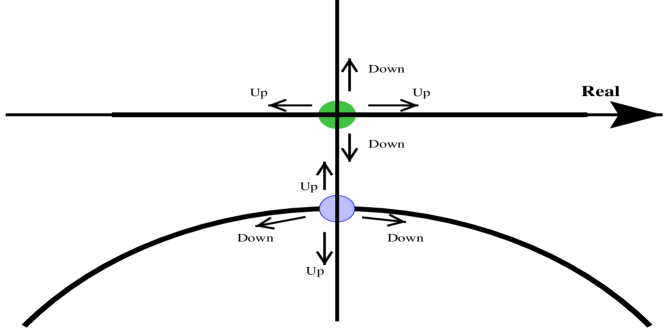
FIG. 1.: Directions of the saddle points used for the zero-dimensional Ising limit of a PT-symmetric theory.

FIG. 2.: Tree graphs of the dual expansion contributing to the asymptotic form of the Green’s functions. Graph (a) is the leading contribution to $G_{2}$, as given in Eq. (82). Graph (b) is the leading contribution to $G_{3}$, and graphs (c) are the two leading contributions to $G_{4}$.

REFERENCES

• [1] E-mail: cmb@howdy.wustl.edu
• [2] E-mail: stb@physics.emory.edu
• [3] E-mail: h.f.jones@ic.ac.uk
• [4] E-mail: pnm@howdy.wustl.edu
• [5] C. M. Bender and S. Boettcher, Phys. Rev. Lett. 80, 5243 (1998).
• [6] C. M. Bender, S. Boettcher, and P. N. Meisinger, J. Math. Phys., 40: 2201, (1999).
• [7] C. M. Bender and S. Boettcher, J. Phys. A: Math. Gen. 31, L273 (1998).
• [8] C. M. Bender, F. Cooper, P. N. Meisinger, and V. M. Savage, Phys. Lett. A, 259, 224-231, (1999).
• [9] C. M. Bender, S. Boettcher, H. F. Jones, and V. M. Savage, J. Phys. A: Math. Gen., 32, 1-11 (1999).
• [10] C. M. Bender, G. V. Dunne and P. N. Meisinger, Phys. Lett. A, 252, 272 (1999).
• [11] A. A. Andrianov, M. V. Ioffe, F. Cannata, J.-P. Dedonder, Int. J. Mod. Phys. A 14, 2675 (1999).
• [12] E. Delabaere and F. Pham, Phys. Lett. A 250, 25 (1998) and 250, 29 (1998).
• [13] E. Delabaere and D. T. Trinh, “Spectral Analysis of the Complex Cubic Oscillator,” University of Nice preprint, 1999.
• [14] M. Znojil, Phys. Lett. A 259, 220 (1999).
• [15] C. M. Bender and G. V. Dunne, J. Math. Phys., 40, 4616-4621, (1999).
• [16] B. Bagchi and R. Roychoudhury, “A New ${\cal PT}$-Symmetric Complex Hamiltonian with a Real Spectrum,” University of Calcutta preprint, 1999.
• [17] F. Cannata, G. Junker, J. Trost, Phys. Lett. A 246, 219 (1998).
• [18] H. Jones, “The Energy Spectrum of Complex Periodic Potentials of the Kronig-Penney Type,” Phys. Lett. A262, 242 (1999).
• [19] C. M. Bender and K. A. Milton, Phys. Rev. D 55, R3255 (1997). There is a factor of 2 error in Eqs. (15) and (16) in this reference which has been corrected in the current paper.
• [20] C. M. Bender and K. A. Milton, Phys. Rev. D 57, 3595 (1998).
• [21] C. M. Bender and K. A. Milton, J. Phys. A: Math. Gen., 32, L87-L92, (1999).
• [22] C. M. Bender and H. F. Jones, “Effective Potential for ${\cal PT}$-Symmetric Quantum Field Theories,” to be published in Foundations of Physics.
• [23] C. M. Bender, K. A. Milton, and V. M. Savage, “Solution of Schwinger-Dyson Equations for ${\cal PT}$-Symmetric Quantum Field Theory,” to be published in Phys. Rev. D.
• [24] P. Dorey and R. Tatao, “On the Relation between Stokes Multipliers and the $T-Q$ Systems of Conformal Field Theory,” University of Durham preprint, 1999.
• [25] C. M. Bender, F. Cooper, G. S. Guralnik, H. Moreno, R. Roskies, and D. H. Sharp, Phys. Rev. Lett. 45, 501 (1980); C. M. Bender and S. Boettcher, Phys. Rev. D 48, 4919 (1993) and 51, 1875 (1994).
• [26] C. M. Bender and S. A. Orszag, Advanced Mathematical Methods for Scientists and Engineers (McGraw-Hill, New York, 1978), Chap. 6.
• [27] A detailed discussion of the rotation of contours for eigenvalue problems is given in C. M. Bender and A. Turbiner, Phys. Lett. A 173, 442 (1993).
Refer to caption