Branes in external field or more about Randall-Sundrum scenario

Abstract

Fate of branes in external fields is reviewed with emphasis on a spontaneous creation of the Brane World. No negative tension brane is involved.

1 Charged Branes

The word ”brane” in this talk will stand for a multidimensional relativistic massive film, possibly charged with respect to an $n$-form (gauge) field. The branes below can be viewed on as the fundamental ones or as effective ones, e.g. domain walls. Its action consists of two pieces, a tension term and a charge term.

Tension term reads

$$S_{tension}=T\oint\sqrt{det({\hat{g}_{ind}})}$$ (1)

the integration is over the brane world-volume, $g_{ind}$ is the metric induced on the world-volume via its embedding into the target space and the coefficient $T$ is the tension of the brane. This term is an analog of the mass term for a particle, $m\oint\sqrt{det({\hat{g}_{ind}})}$, where integration is over world-line of the particle.
Charge term reads

$$S_{charge}=e\oint{B},$$ (2)

where ${B}$ is a $n$-form gauge field field, corresponding curvature being $H=dB$. Branes are sources for this field and they are affected by this field. In what follows we assume $H$ to be a top degree form.

Everything I am going to talk about is related to the Schwinger type process - production of branes by homogeneous external field $H$.

2 A warm up example

Consider first a warm up example: production of particles by a homogeneous $E$ field.

For this case the effective action reads

$$S_{eff}=TL-eEA$$ (3)

where $L$ is the length of the world-line of the particles produced, $T$ is a mass of the particle, (as usual, particle-antiparticle history looks like a closed world-line), and $A$ is the area surrounded by the world-line.

Notice, by the way, that upon appropriate identification of the parameters, the same effective action describes false vacuum decay in (1+1) scalar field theory. Particles are substituted by kinks, electric field - by energy difference between false and true vacuum.

Extremal world-line for the action Eq.(3) is a circle of the radius ${\bar{r}}=\frac{T}{eE}$.

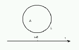
Figure 1: Euclidean bounce for particle production.

Value of the effective action on this extremal curve (bounce) defines the probability P of the spontaneous process: follows

$$P\propto exp(-\frac{\pi T^{2}}{eE}).$$ (4)

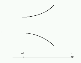
Figure 2: Minkowski evolution of the particles produced.

Notice that Minkowski evolution is obtained from the Euclidean bounce by analitical continuation.

3 Spontaneous production of branes

The above warm-up example is easily generalized to the case of spontaneous production of branes in a homogeneous $H$ field [1]. The effective action in the assumption of homogeneouty of $H$ reads

$$S_{eff}=TA-ehV.$$ (5)

World-volume of the brane produced form a closed hypersurface (like the world-line of the particle produced in the above example). $A$ in Eq.(5) is the area of the world-volume, $V$ - volume of the region inside the brane. The Euclidean bounce is a $p+1$-dimensional sphere of radius $\bar{r}=\frac{(d-1)T}{eh}$. The value of the effective action on the bounce defines probability of the brane production:

$$P\propto exp(-const\frac{T^{d}}{(eh)^{d-1}}).$$ (6)

Analogously to the above example, The Minkowski evolution can be obtained from the Euclidean bounce via analytical continuation.

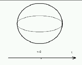
Figure 3: Euclidean bounce for brane production.

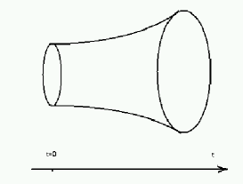
Figure 4: Minkowski evolution of the brane produced.

For branes it is important to include gravity, which also was done in [1] and which I’ll be back later on in my talk.

4 Induced brane production

Let us now consider the induced brane production [2]. Before doing so, I need to introduce a new ingredient - brane junctions [3]. Brane world-volumes can meet. The manifold along which the world-volumes meet is called the junction manifold. Angles at which the branes meet each other are fixed by the tension force balance condition. And, of course, charge of the branes is conserved. That was about junctions.

The setup for the induced brane production is as follows. There is external homogeneous field and there is external neutral brane which can have junctions with charged branes to be produced. The question is what is the probability.

Let us again begin with a warm up example - one particle induced decay in (1+1)d [4]. The setup is as follows. On has a false vacuum and a massive particle in it such that the correspondig field has a zero mode on the wall which could separate false and true vacuum. Then, if a bubble of the true vacuum vacuum inside the false vacuum is produced, it is more profitable for the particle to ride a part of its way in the form of zero mode on the wall of the bubble. Th effective action describing this case,

$$S_{eff}=mL-eEA+m{\tilde{L}},$$ (7)

differs from Eq.(3) only by the last term. $m$ is the mass of the extra particle, ${\tilde{L}}$ is the length of the extra particle world-line (only outside the bubble).

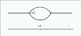
Figure 5: Bounce for the induced vacuum decay.

The bounce is now glued of two segments of a circle of the same radius as in the case of spontaneous decay. These two segments meet with the world-line of the particle (junction!) at the angle $\alpha$ which is defined by the force balance condition, $m=2T\cos\alpha$.

The ”charge conservation” in the present case is equivalent to a trivial fact that when one passes through the bubble crossing its wall twice, one gets back to false vacuum. One then straightforwardly compute the probability of the false vacuum decay [4]. There are two clear limiting cases. When mass of the particle is small compared to the mass of the wall, bounce is not disturted and probability is the same in spontaneous case. When mass of the particle is close to $2T$, bounce shrinks to a point and there is no exponential suppression in the induced vacuum decay.

Generalization to the case of branes is more or less obvious [2].

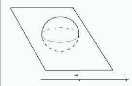
Figure 6: Bounce for the induced brane production.

The bounce now consists of two segments of (d-1) dimensional sphere of the same radius as in the case of spontaneous brane production, glued to the external brane along the junction manifold. The force balance condition reads ${\tilde{T}}=2T\cos\alpha$, where ${\tilde{T}}$ is the tension of the external neutral brane. Minkowski evolution is again obtained by analytical continuation of the bounce.

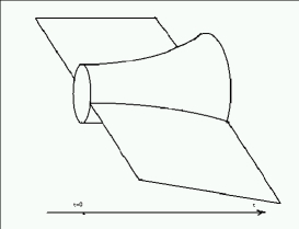
Figure 7: Minkowski evolution for the induced brane production.

Calculation of the probability is straightforward, two clear limiting cases are as in the warm up example.

5 A sketch of Brane World

Now I would like to make a digression to sketch an idea of the Brane World. This is an alternative to the idea of compactification. In compactification extra dimensions are compact and small and thus cannot be seen at moderate energies. In the brane world, extra dimensions are infinite, but the matter [5], gauge fields [6] and gravity [7] are localized on a brane (domain wall or other topological defect in the extra dimensions).

The model considered in [7] included two branes localized at different points on a circle (the 5th dimension was taken $S^{1}$ of arbitrarily large radius). One of the branes was physical (RS-brane), the other was a so-called regulator brane (R-brane). The gravity was localized on the RS brane. The drawback of the model was that R-brane had a negative tension (see e.g. discussion in [8]).

Many modifications of the construction in [7] were studied (see e.g. [9] and other references to the original paper [7]), most of them included the negative tension brane.

Let us consider in more detail the construction in [10].

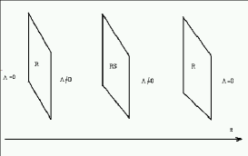
Figure 8: Gregory-Rubakov-Sibiryakov model.

It included three branes localized on a line (5th dimension was taken $R^{1}$), two negative tension R-branes and one RS-brane between them. Cosmological constant outside R-branes was zero, cosmological constant between R-branes and RS-brane was negative. Notice that in this model cosmological constant is not really a constant, it jumps on the R-branes. So, in fact, there is a hidden external field in the model, and R-branes are charged with respect to it. This motivates the following construction in [11].

6 Spontaneous Brane World creation

I would now like to describe spontaneous creation of the Brane world in a homogeneous external field. The process considered is a sort of inverse to the induced brane production in the external field. The bounce now consists of two segments of the charged branes (R-branes) which are glued along the junction manifold with the neutral brane (RS-brane) which is inside the bubble.

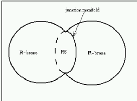
Figure 9: Tunneling into the Brane World.

The relevant effective action reads

$$S=\frac{1}{2k}\int d^{5}x\sqrt{g}(-R+2\Lambda)+\frac{1}{k}\oint\sqrt{g}_{ind}K+$$

$$\frac{1}{2}\int d^{5}x\sqrt{g}h^{2}+T_{R}\oint_{R}\sqrt{g}_{ind}+T_{RS}\oint_{RS}\sqrt{g}_{ind}$$ (8)

Let us explain ingredients in Eq.(6). $h$ is Hodge dual scalar of the field strength $H$. Being a top form, this field does not propagate. Field equations say that in empty space $h$ is a constant, in our case it only jumps at the charged R-branes by its charge e, $h_{+}-h_{-}=e$, where $h_{+}$ is outside value of $h$, $h_{-}$ is its inside value. In the effective action Eq.(6) it is assumed that field equations for $h$ are resolved, the charge of the R-branes enters effective action only via $h^{2}$-term.

Constant k in Eq.(6) is the five dimensional gravitational constant, $R$ - scalar curvature, $\Lambda$ stands for cosmological constant, for which we assume that it is negative and exactly compensates energy density of the field $h$ outside, $\Lambda+\frac{kh_{+}^{2}}{2}=0$ so that outside the metric is flat. Notice right away that effective cosmological constant inside is

$$\Lambda_{eff}=\Lambda+\frac{kh_{-}^{2}}{2}=-\frac{kh_{+}^{2}}{2}+\frac{kh_{-}^{2}}{2}.$$ (9)

and hence the scalar curvature $R$ of the AdS metric inside any of the two segments in figure reads $R=\frac{2d}{d-2}\Lambda_{eff}=\frac{10}{3}\Lambda_{eff}$, and the corresponding AdS radius, $R_{AdS}$, reads $R^{2}_{AdS}=-\frac{2(d-1)(d-2)}{\Lambda_{eff}}=-\frac{24}{\Lambda_{eff}}$.

The origin of two of the three surface terms in Eq.(6) is obvious - these are tension terms for R- and RS-branes. The third term, $\frac{1}{k}\oint\sqrt{g}_{ind}K$ is introduced to ensure that variation of the curvature term does not depend on normal derivatives of variation of the metric on the branes [12]. Here $K=g_{ind}^{ij}K_{ij}$ stands for the trace of the external curvature $K_{ij}$ of the branes, the integral is over all branes, every brane contributing twice, with $K$ computed in metric on one or the other side of the brane.

So much about ingredients in the effective action Eq.(6). Let us now explain details of the bounce solution. The metric to the right of the RS-brane inside R-brane reads

$$ds^{2}=\frac{dz^{2}+d\rho^{2}+\rho^{2}d\Omega^{2}_{3}}{(1-\frac{(z-a)^{2}+\rho^{2}}{R^{2}_{AdS}})^{2}}$$ (10)

while the metric to the left of the RS-brane inside R-brane reads

$$ds^{2}=\frac{dz^{2}+d\rho^{2}+\rho^{2}d\Omega^{2}_{3}}{(1-\frac{(z+a)^{2}+\rho^{2}}{R^{2}_{AdS}})^{2}}$$ (11)

where $z$ is coordinate along the axes of symmetry orthogonal to RS-brane, $\rho$ is the radial coordinate in orthogonal to $z$ directions, $d\Omega^{2}_{3}$ is the metric of the corresponding 3-sphere, $a$ is a parameter.

The metrics Eq.(10),(11) are to be sewed on R-branes with flat metric and on RS-brane with each other, in the sence that metrics themselves are continues, while their normal derivatives jump according to the Israel condition, $\Delta K_{ij}=\frac{kT}{d-1}g_{ij}=\frac{kT}{4}g_{ij}$. On R-branes this condition fixes radius ${\bar{R}}$ of the spherical segments, ${\bar{R}}=\frac{2T_{R}(d-1)}{h^{2}_{+}-h^{2}_{-}}$, which is of course the same as for bounce without RS-brane, and on RS-brane this condition fixes the parameter $a$, $a=\frac{T_{RS}(d-1)}{h^{2}_{+}-h^{2}_{-}}$. Importantly, $cos{\alpha}=\frac{a}{\bar{R}}=\frac{T_{RS}}{2T_{R}}$, which is precisely the force balance condition at the junctions.

Substituting these data into the effective action Eq.(6) one straigtforwardly obtains exponential factor for the probability P of the process. It ranges between $P\propto e^{-S_{bt}}$ for very light RS-brane, $T_{RS}\ll T_{R}$, where $S_{bt}$ is the action for the bounce without RS-brane, which has been computed in [1], and $P\propto e^{-2S_{bt}}$ for $T_{RS}=2T_{R}$. More heavy RS-brane cannot be produced in this way.

Since the internal brane is located at $z=0$ the induced metric of 4D world is immediately seen from Eq.(10). It appears to be the AdS space with the AdS radius $R_{AdS4}^{2}=R_{AdS}^{2}-a^{2}$ and, correspondingly, the cosmological constant $\Lambda_{4}=-\frac{12}{(R_{AdS}^{2}-a^{2})}$

After continuation into Minkowski space our Universe is a spacially finite, growing slice of AdS space. Spacial radius of R-brane is also growing, and we are eventually left with the picture of [7], or [10], type.

7 Some other related solution

I would also like to describe some other related solution obtained in[11].

Interestingly, one can have multiple RS branes in the final state. In that case we have additional pair of the R brane segments of the same radius $\bar{R}$ for each new RS brane. The metric between the n-th and n+1 -th RS branes reads

$$ds^{2}_{n}=\frac{dz^{2}+d\rho^{2}+\rho^{2}d\Omega^{2}_{3}}{(1-\frac{(z-a_{n})^{2}+\rho^{2}}{R^{2}_{AdS}})^{2}}$$ (12)

where $a_{n}=(2n-1)a$. We choose z=0 at the center of the left R brane segment.

The distance between branes in fifth dimension is $\delta x_{5}=2a$. Let us interpret the RS branes as D branes which are neutral with respect to the external NS field. The picture described would amount to the generic U(N) gauge group on their worldvolume. Let us note that since the distance between branes can be interpreted as the vacuum expectation values of the scalar field on the worldvolume of D branes we have no moduli associated to scalars in this solution.

8 Conclusion

My conclusions are as follows:
1. We have described induced brane production in external field;
2. We have described tunneling into the Brane World (a sort of Big Bang);
3. No negative tension branes;
4. 5d early Universe;
5. non-flat (AdS) 4d brane - curable (see [13]).

I am thankful to A.Gorsky for the fruitful collaboration.

References

- [1] J. D. Brown and C. Teitelboim, Nucl. Phys. B297, 787 (1988).
- [2] A. Gorsky and K. Selivanov, Nucl. Phys. B571, 120 (2000) [hep-th/9904041].
- [3] J. Schwarz, Nucl. Phys. (Proc. Suppl) B55 (1997).
- [4] K. G. Selivanov and M. B. Voloshin, JETP Lett. 42, 422 (1985).
-
[5]
V. A. Rubakov and M. E. Shaposhnikov,
Phys. Lett. B125 (1983) 136.
K. Akama,“An early proposal of ’brane world’,”Lecture Notes in Physics, 176, (Springer-Verlag, 1983), 267-271, hep-th/0001113. -
[6]
J. Polchinski, Phys. Rev. Lett. 75 (1995),4724
E. Witten, Nucl. Phys. B460 (1996) 335 - [7] L. Randall and R. Sundrum, Phys. Rev. Lett. 83, 4690 (1999) [hep-th/9906064].
- [8] E. Witten,hep-ph/000229.
-
[9]
I. I. Kogan, S. Mouslopoulos, A. Papazoglou, G. G. Ross and J. Santiago,
hep-ph/9912552.
I. I. Kogan and G. G. Ross,hep-th/0003074.
G. Dvali, G. Gabadadze and M. Porrati,hep-th/0002190
C. Csaki, J. Erlich and T. J. Hollowood,hep-th/0002161. - [10] R. Gregory, V. A. Rubakov and S. M. Sibiryakov, hep-th/0002072.
- [11] A. Gorsky and K. Selivanov, Phys.Lett.B485 (2000) 271, hep-th/0005066.
- [12] W. Israel, Nuovo Cim. 44B (1966) 1; 48B (1967) 463
- [13] A. Gorsky and K. Selivanov, hep-th/0006044