Quantized Einstein-Rosen waves, ${\rm AdS}_{2}$,
and spontaneous symmetry breaking

Max Niedermaier
Department of Physics

100 Allen Hall, University of Pittsburgh

Pittsburgh, PA 15260, USA

Abstract

4D cylindrical gravitational waves with aligned polarizations (Einstein-Rosen waves) are shown to be described by a weight $1/2$ massive free field on the double cover of ${\rm AdS}_{2}$. Thorn’s C-energy is one of the $sl(2,\mbox{\rm IR})$ generators, the reconstruction from the (timelike) symmetry axis is the ${\rm CFT}_{1}$ holography. Classically the phase space is also invariant under a O(1,1) group action on the metric coefficients that is a remnant of the original 4D diffeomorphism invariance. In the quantum theory this symmetry is found to be spontaneously broken while the ${\rm AdS}_{2}$ conformal invariance remains intact.

Introduction: The Einstein-Rosen (ER) subsector of general relativity provides a simple, yet instructive, laboratory for studying certain quantum aspects of gravity [1, 2, 3]. In brief, ER-waves are gravitational wave solutions to the Einstein equations with cylindrical symmetry and aligned polarizations. In Weyl-canonical coordinates the 4-dim. line element can locally be written in the form

$$ds^{2}=e^{\gamma-\phi}(dt^{2}-dr^{2})-(e^{\phi}dz^{2}+r^{2}e^{-\phi}d\alpha^{2})\;,$$ (1)

where $\phi$ and $\gamma$ are functions of $t,r$ and $z,\alpha$ are the coordinates along the orbits of the two Killing vector fields. Einstein’s equations turn out simply to be equivalent to a spherical wave equation for $\phi$, i.e. $[\partial_{t}^{2}-\partial_{r}^{2}-\frac{1}{r}\partial_{r}]\phi=0$, together with the condition that $\gamma$ is expressed in terms of $\phi$ by

$$\gamma(t,r^{\prime})=\frac{1}{2}\int_{0}^{r^{\prime}}drr[(\partial_{t}\phi)^{2}+(\partial_{r}\phi)^{2}]\;,$$ (2)

The conserved quantity $\gamma_{\infty}=\gamma(t,\infty)$ is known as Thorn’s C-energy while the physical Hamiltonian is $1-e^{-\gamma_{\infty}/2}$ [11], and measures a 3D deficit angle.

The Killing vector fields $\frac{\partial}{\partial z}$, $\frac{\partial}{\partial\alpha}$ of course are unique only up to normalization. A constant rescaling of the coordinates $z\rightarrow e^{-\lambda/2}z,\;\alpha\rightarrow e^{\lambda/2}\alpha$, $\lambda\in\mbox{\rm IR}$, amounts to changing their norm, which can be compensated by $\phi(t,r)\rightarrow\phi(t,r)+\lambda$. For the combinations of the metric coefficients ${\rm ch}\phi$ and ${\rm sh}\phi$ the shift amounts to a linear transformation by an element of the non-compact Lie group O(1,1), which can be seen to be a symmetry of the classical phase space. Adopting the quantization scheme of [2] we shall later find this symmetry to be spontaneously broken in the quantum theory.

In the $(t,r)$ part of the line element (1) the shift $\phi(t,r)\rightarrow\phi(t,r)+\lambda$ can be compensated by a rescaling $t\rightarrow e^{\lambda/2}t,\,r\rightarrow e^{\lambda/2}r$. Together with the time translations this generates a Borel subgroup of $SL(2,\mbox{\rm IR})$, which classically can be promoted to a symmetry of (1). Although the “targetspace” O(1,1) symmetry is spontaneously broken in the quantum theory, the dilatation symmetry $t\rightarrow e^{\lambda/2}t,\,r\rightarrow e^{\lambda/2}r$ turns out to remain intact, and is unitarily implemented by a generator $H$. In particular this gives rise to a thermalization phenomenon akin to the the Unruh effect: Restricting the quantum theory to the cone $t\geq r\geq 0$, the ground state for $\gamma_{\infty}$ (generating the $t$-evolution) is a thermal state for the dilatation-evolution, of temperature $1/2\pi$. From the 4D viewpoint the restricted theory can be regarded as the quantum theory of those “exotic” ER-waves whose scalar $\phi(t,r)$ has support for $t\geq r\geq 0$ only. On the level of the Lie algebra, the symmetry can further be extended to a full $sl(2,\mbox{\rm IR})$ action on the $(t,r)$ “worldsheet”, whose generators $E=\gamma_{\infty}/2,\,H$ and $F$ are local conserved charges that leave the vacuum invariant. The corresponding finite transformations however will be symmetries of the (classical and quantum) theory only if the $(t,r)$ Lorentzian space is extended to the double cover of two-dimensional Anti-deSitter space, ${\rm AdS}_{2}$. Without the extension the ER-system would also not allow for a CPT operation. Taking advantage of the ${\rm AdS}_{2}$ extension, the ${\rm AdS}_{2}/{\rm CFT}_{1}$ correspondence then yields a quantum version of the known classical reconstruction [12] from the $r=0$ symmetry axis.

Spontaneous breakdown of O(1,1) symmetry: The quantum theory of ER-waves descends from that of a free scalar field $\Phi=\sqrt{r}\phi$ having the following expansion in terms of Bessel functions (see e.g. [2])

$$\Phi(t,r)=\int_{0}^{\infty}d\omega\sqrt{\frac{r}{2}}J_{0}(\omega r)\left[A(\omega)e^{-i\omega t}+A^{\dagger}(\omega)e^{i\omega t}\right]\;,$$

$$[A(\omega),A^{\dagger}(\omega^{\prime})]=\delta(\omega-\omega^{\prime})\;.$$ (3)

It is readily identified as that of a weight $h=1/2$ massive free field on ${\rm AdS}_{2}$. Indeed in Poincaré coordinates $(t,r)$ the wave equation on ${\rm AdS}_{2}$ is (see e.g. [4, 5])

$$\big{\{}\Box_{AdS_{2}}+h(h-1)\big{\}}\varphi(t,r)=0\;,\makebox[28.45274pt]{ }\Box_{AdS_{2}}=r^{2}(\partial_{t}^{2}-\partial_{r}^{2})\;,$$ (4)

where $h\geq 1/2$ parameterizes the mass via $m^{2}=h(h-1)$, and $h=1/2$ is the unitarity threshold. For $h=1/2$ one obtains the expansion (3) in terms of positive and negative frequency solutions. The shift invariance $\phi(t,r)\rightarrow\phi(t,r)+\lambda$ reflects the ambiguity in the zero mode contribution proportional to $\sqrt{r}$ in (3). The $(t,r)$ coordinates cover only part of ${\rm AdS}_{2}$; we shall describe later why the extension to the double cover of ${\rm AdS}_{2}$ is mandatory in this context.

For the discussion of symmetry breaking it is more useful to regard (3) as the spherical reduction of a 1+2 dim. massless scalar field. Recalling the positive frequency two-point function of the latter

$$W_{3}(x)=\frac{1}{4\pi}\left[{\theta}(x^{2})\frac{{\rm sign(x_{0})}}{\sqrt{x^{2}}}+i{\theta}(-x^{2})\frac{1}{\sqrt{-x^{2}}}\right]\,,\quad x^{2}=x_{0}^{2}-x_{1}^{2}-x_{2}^{2}\,,$$ (5)

and switching to angular coordinates in the $x_{1},x_{2}$ plane, the two-point function of $\Phi(t,r)$ in the Fock vacuum $A(\omega)|0\rangle=0$, can be written as

$$W(t_{1}-t_{2};r_{1},r_{2}) \!=\! i\langle 0|\Phi(t_{1},r_{1})\,\Phi(t_{2},r_{2})|0\rangle=\sqrt{r_{1}r_{2}}\int_{-\pi}^{\pi}d\alpha\,W_{3}(t_{1}-t_{2};r_{1},r_{2};\alpha)\;,$$ (6)

in an obvious notation for the integrand. The integrations in (6) can be reduced to complete elliptic integrals ${\bf K}(u)=\int_{0}^{\pi/2}d\alpha(1-u\sin^{2}\alpha)^{-1/2}$. The result is

$$W(t_{1}-t_{2};r_{1},r_{2})=\frac{1}{2}{\rm sign}(t_{1}-t_{2})\,d(\xi^{2})+\frac{i}{2}\,d(1-\xi^{2})\;,$$ (7)

where $\xi^{2}=[(t_{1}-t_{2})^{2}-(r_{1}-r_{2})^{2}]/(4r_{1}r_{2})$ is the ${\rm AdS}_{2}$ invariant distance in Poincaré coordinates. The function $d(u)$ is given by $d(u)=0$ for $u<0$ and

$$d(u)={\theta}(1-u)\frac{1}{\pi}\,{\bf K}(u)+{\theta}(u-1)\frac{1}{\pi\sqrt{u}}\,{\bf K}(1/u)\,,\quad u\geq 0\;.$$ (8)

Up to a sign $d(\xi^{2})$ coincides with the commutator function $2{\rm Re}\,W$; a plot of $d(\xi^{2})$ is shown below. Large and small distances are related by the duality $d(1/\xi^{2})=\sqrt{\xi^{2}}\,d(\xi^{2})$. The limits are: $\lim_{\xi^{2}\rightarrow 0^{+}}d(\xi^{2})=1/2$ and $d(\xi^{2})\sim 1/2\sqrt{\xi^{2}}$, for $\xi^{2}\rightarrow\infty$. Note that rather than being singular on the 1+1 dim. lightcone $\xi^{2}=0$, $d(\xi^{2})$ is singular at $\xi^{2}=1$, i.e. $|t_{1}-t_{2}|=r_{1}+r_{2}$. The behavior across the $1+1$ dim. lightcone is discontinuous, but with a finite jump.

Figure 1: Commutator function of the ER-scalar

Classically the symmetry $\Phi(t,r)\rightarrow\Phi(t,r)+\lambda\sqrt{r}$ is generated by the conserved charge $Q=i\int_{0}^{\infty}dr\sqrt{r}\partial_{t}\Phi$. In the quantum theory, following the standard procedure [8], one will try to define $Q$ as a suitable limit of regularized operators $Q_{R}$ (supported in a sphere of radius $R$), as $R\rightarrow\infty$. The symmetry associated with the current is said to be spontaneously broken, if the limit of the commutator’s vacuum expectation value $q:=\lim_{R\rightarrow\infty}(\Omega,[Q_{R},A(x)]\Omega)\;(*)$ is a non-zero number, independent of the regulators, for some $A(x)$. In this case the limit of the operators $Q_{R}$ does not define the generator of a unitary group of automorphisms which induces the symmetry transformations and leaves the vacuum invariant. For the application to the ER-waves it is important that this criterion has a functional analytical origin [8] and does not hinge e.g. on Poincaré invariance. In a Minkowski space quantum field theory it is known that $q\neq 0$ can only occur in the presence of massless 1-particle states. Indeed the prototype example for $(*)$ to hold with $q\neq 0$ is the current $i\partial_{0}\phi$ of a massless free scalar field in $d\geq 3$ spacetime dimensions, taking for $A(x)$ the scalar field $\phi(x)$ itself. The symmetry broken is $\phi(x)\rightarrow\phi(x)+\lambda$. In $d=2$ this result does not apply because the massless commutator function fails to comply with the Wightman axioms, – which is one way of understanding the absence of spontaneous symmetry breaking in two dimensions [9].

In view of (5), (6) the ER-scalar lies in-between the 2+1 dim. and the 1+1 dim. situation and the issue has to be examined from scratch. To do so, one first verifies that for every operator $A$ in the polynomial field algebra of $\Phi$ the commutator $[Q_{R},A]$ is independent of $g_{R}$ and $f$ for sufficiently large $R$, where

$$Q_{R}=i\int dtdr\sqrt{r}f(t)g_{R}(r)\,\partial_{t}\Phi(t,r)\;,$$ (9)

and $g_{R}$ is a smooth function with $g_{R}(r)=1$ for $r\in[R^{-1},R]$, rapidly decaying for $r\rightarrow 0$ and $r\rightarrow\infty$, and $\int dtf(t)=1$. The independence of $g_{R}$ follows from the vanishing of the commutator function $2{\rm Re}W$ at spacelike 1+1-dim. distances; the independence from $f$ is a consequence of current conservation. The attempt to define a hermitian charge operator along the above lines requires that the commutator with $\Phi$ has vanishing vacuum expectation value for sufficiently large $R$. However one straightforwardly verifies

$$\langle 0|[Q_{R},\Phi(t_{2},r_{2})]|0\rangle=\sqrt{r_{2}}\;,\quad\mbox{for $R$ large}\;,$$ (10)

establishing that the transformation $\Phi(t,r)\rightarrow\Phi(t,r)+\lambda\sqrt{r}$ cannot be unitarily implemented on the Fock space. It is crucial here that the commutator function is a well-defined ${\rm AdS}_{2}$-invariant distribution so that no caveat arises as in the case of a relativistic massless field in 1+1 dim. Minkowski space; c.f. [9]. An analogous symmetry breaking has already been found in the situation with generic polarizations [13] by very different means.

Unbroken $sl(2,\mbox{\rm IR})$ symmetry: The field eq. (4) follows from an obvious action, which can be verified to be separately invariant under the variations $\delta_{e}\Phi=-i{\bf e}\Phi$, $\delta_{h}\Phi=-i{\bf h}\Phi$, $\delta_{f}\Phi=-i{\bf f}\Phi$. Here ${\bf e},{\bf h},{\bf f}$ generate a realization of $sl(2,\mbox{\rm IR})$ in terms of differential operators ${\bf e}=\partial_{t},\,{\bf h}=2(t\partial_{t}+r\partial_{r}),\,{\bf f}=-(t^{2}+r^{2})\partial_{t}-2tr\partial_{r}$, acting on a suitable space of test functions. In particular they are anti-hermitian wrt the measure $\int dtdt/r^{2}$. The quadratic Casimir is ${\bf C}=-\Box_{AdS_{2}}$, so that the operator equation of motion for $\Phi$ amounts to ${\bf C}=h(h-1)|_{h=1/2}\mbox{11}=-1/4\mbox{11}$. The Noether currents $J_{\mu}({\bf e}),J_{\mu}({\bf h}),J_{\mu}({\bf f})$ associated with the above $sl(2,\mbox{\rm IR})$ variations are

$$\begin{array}[]{ll}J_{t}({\bf e})=(\partial_{t}\Phi)^{2}+(\partial_{r}\Phi)^{2}-\frac{1}{4r^{2}}\Phi^{2}\;,&J_{r}({\bf e})=2\partial_{r}\Phi\partial_{t}\Phi\;,\\[5.69054pt] J_{t}({\bf h})=2tJ_{t}({\bf e})+2rJ_{r}({\bf e})\;,&J_{r}({\bf h})=2r[J_{t}({\bf e})+\frac{1}{2r^{2}}\Phi^{2}]+2tJ_{r}({\bf e})\;,\\[5.69054pt] J_{t}({\bf f})=-(t^{2}+r^{2})J_{t}({\bf e})-2trJ_{r}({\bf e})\;,&J_{r}({\bf f})=-2tr[J_{t}({\bf e})+\frac{1}{2r^{2}}\Phi^{2}]-(t^{2}+r^{2})J_{r}({\bf e})\,.\end{array}$$ (14)

In (14) we omitted total derivative terms in order to simplify the expressions. Restoring them is however essential to arrive at the correct classical Noether charges. In the quantum theory normal ordering is understood. Repeating the previous analysis for these charges, one finds that this symmetry is unbroken and is implemented by hermitian operators $E,H,F$ that annihilate the vacuum. They satisfy $[E,\Phi(t,r)]=-i{\bf e}\Phi(t,r)$, etc., and generate the expected $sl(2,\mbox{\rm IR})$ algebra: $[H,E]=-2iE,\,[F,E]=iH,\,[H,F]=2iF$. Explicitly

$$\begin{array}[]{ll}\displaystyle{E=\int_{0}^{\infty}d\omega A^{\dagger}(\omega)\,ie(\omega)A(\omega)}\;,&e(\omega)=-i\omega\;,\\[5.69054pt] \displaystyle{H=\int_{0}^{\infty}d\omega A^{\dagger}(\omega)\,ih(\omega)A(\omega)}\;,&h(\omega)=-(2\omega\partial_{\omega}+1)\;,\\[5.69054pt] \displaystyle{F=\int_{0}^{\infty}d\omega A^{\dagger}(\omega)\,if(\omega)A(\omega)}\;,&\,f(\omega)=-i(\omega\partial^{2}_{\omega}+\partial_{\omega})\;.\end{array}$$ (18)

Here $e(\omega),\,h(\omega),\,f(\omega)$ again form an anti-hermitian realization of $sl(2,\mbox{\rm IR})$, now with constant Casimir $C(\omega)=-1/4$. In particular $2E$ yields a quantum version of the C-energy $\gamma_{\infty}$ [2]. Exponentiating this $sl(2,\mbox{\rm IR})$ action yields

$$\begin{array}[]{lll}\displaystyle{e^{isE}A^{\dagger}(\omega)e^{-isE}}&\!\!=\displaystyle{e^{-se(\omega)}A^{\dagger}(\omega)}&\!\!=\displaystyle{e^{is\omega}A^{\dagger}(\omega)}\;,\\[7.11317pt] \displaystyle{e^{isH}A^{\dagger}(\omega)e^{-isH}}&\!\!=\displaystyle{e^{sh(\omega)}A^{\dagger}(\omega)}&\!\!=\displaystyle{e^{-s}A^{\dagger}(e^{-2s}\omega)}\;,\\[5.69054pt] \displaystyle{e^{isF}A^{\dagger}(\omega)e^{-isF}}&\!\!=\displaystyle{e^{-sf(\omega)}A^{\dagger}(\omega)}&\!\!=\displaystyle{-\frac{i}{s}\int_{0}^{\infty}d\lambda\,J_{0}\left(\frac{2}{s}\sqrt{\omega\lambda}\right)\!e^{\frac{i}{s}(\omega+\lambda)}A^{\dagger}(\lambda)}\;.\end{array}$$ (22)

Together the 1-parameter families (22) generate a unitary representation $SL(2,\mbox{\rm IR})\ni g\rightarrow U(g)$ on the Fock space. The 1-particle subspace of the Fock space is irreducible wrt this $SL(2,\mbox{\rm IR})$ action; see e.g. [10]. The action of $U(g)$ is best described in terms of the Laplace transforms

$$\!\!\!A^{-}({\theta})=\frac{1}{\sqrt{2}}\int_{0}^{\infty}\!d\omega A(\omega)e^{-i\omega{\theta}},\;{\rm Im}\,{\theta}<0\;,\quad A^{+}({\theta})=\frac{1}{\sqrt{2}}\int_{0}^{\infty}\!d\omega A^{\dagger}(\omega)e^{i\omega{\theta}},\;{\rm Im}\,{\theta}>0\,,$$ (23)

(both supposed to vanish in the other half plane) and reads

$$U(g)A^{\pm}({\theta})U(g)^{-1}=\frac{A^{\pm}({\theta}^{g})}{c{\theta}+d}\;,\makebox[28.45274pt]{ }{\theta}^{g}=\frac{a{\theta}+b}{c{\theta}+d}\;,\quad g={a\;\;b\choose c\;\;d}\in SL(2,\mbox{\rm IR})\;.$$ (24)

We take $\phi^{b}(t)=\lim_{{\epsilon}\rightarrow 0}\,[A^{-}(t-i{\epsilon})+A^{+}(t+i{\epsilon})]$ as the definition of the (classical and quantum) field on the $r=0$ symmetry axis. In a distributional sense $\phi^{b}(t)$ inherits the transformation law (24). The two-point function on the axis

$$\lim_{r\rightarrow 0}\frac{1}{r}W(t_{1}-t_{2};r,r)=\frac{1}{2(t_{1}-t_{2})}=i\,\langle 0|\phi^{b}(t_{1})\phi^{b}(t_{2})|0\rangle\;,$$ (25)

is well-defined and covariant. The boundary field $\phi^{b}(t)$ is of additional interest because $\phi(t,r)$ can be uniquely reconstructed from it. Indeed, using the Laplace transforms (23) one can rewrite the expansion (3) as

$$\phi(t,r) \!=\! \frac{1}{2\pi}\int_{t-r}^{t+r}d{\theta}\frac{1}{\sqrt{r^{2}-(t-{\theta})^{2}}}\,[A^{+}({\theta})+A^{-}({\theta})]$$ (26)

$$+ \frac{i}{2\pi}\left(\int_{-\infty}^{t-r}d{\theta}-\int_{t+r}^{\infty}d{\theta}\right)\frac{1}{\sqrt{(t-{\theta})^{2}-r^{2}}}\,[A^{+}({\theta})-A^{-}({\theta})]\;.$$

The terms in square brackets can be identified as the field on the axis and its Hilbert transform

$$A^{+}({\theta})+A^{-}({\theta})=\phi^{b}({\theta})\;,\makebox[28.45274pt]{ }A^{+}({\theta})-A^{-}({\theta})=\frac{1}{i\pi}\,{\cal P}\!\!\int_{-\infty}^{\infty}dt\,\frac{\phi^{b}(t)}{t-{\theta}}\;.$$ (27)

Thus (26) allows one to reconstruct the field entirely from its values on the $t$-axis. In contrast to the Cauchy problem only one function has to be prescribed.

The finite transformations generated by the exponentials of ${\bf e},\,{\bf h},\,{\bf f}$ are Moebius transformations in the null coordinates $t\pm r$, i.e.

$$t\pm r\ \longrightarrow\ (t\pm r)^{g}=\frac{a(t\pm r)+b}{c(t\pm r)+d}\;,\quad ad-bc=1\;.$$ (28)

They leave the line element $ds^{2}=(dt^{2}-dr^{2})/r^{2}$ and the Casimir operator in (4) invariant. Thus, although for $c\neq 0$ they no longer preserve the Weyl-canonical form of the line element (1), they in principle map solutions of the field equations into themselves. However outside some save regions (like the $t$-axis or the cone $t\geq r\geq 0$ for $cd>0$) transformations with $c\neq 0$ can map positive $r$ and positive $t^{2}-r^{2}$ into negative ones, and can also ruin the hermiticity of the transformed field $\phi$. Such problems are known to be a generic feature of conformal quantum field theories and the resolution is to switch to a suitable covering manifold (see e.g. [6] in the original, and [5] in the AdS context). In the case at hand one is lead to the double cover of ${\rm AdS}_{2}$.

${\rm AdS}_{2}$ and $SU(1,1)$ action: The universal cover of ${\rm AdS}_{2}$ can be described in terms of coordinates $(\tau,\sigma)$ in which the line element takes the form $ds^{2}=(d\tau^{2}-d\sigma^{2})/\cos^{2}\sigma$, with $-\frac{\pi}{2}\leq\sigma<\frac{\pi}{2}$, $-\infty<\tau<\infty$. Spatial infinity is at $\sigma=\pm\frac{\pi}{2}$, the segment $-\pi<\tau<\pi$ is called the primitive domain. The invariant distance is

$$\xi_{G}^{2}=\frac{\cos(\sigma_{1}-\sigma_{2})-\cos(\tau_{1}-\tau_{2})}{2\cos\sigma_{1}\cos\sigma_{2}}\;.$$ (29)

The projection onto ${\rm AdS}_{2}$ is effected by identifying the points $(\tau,\sigma)$ and $(\tau+\pi,-\sigma)$. The previously used Poincaré coordinates $(t,r)$ cover only the patch $\tau+\sigma<\frac{\pi}{2}$ and $\tau-\sigma>-\frac{\pi}{2}$ in the primitive domain; c.f. Fig. 2 below. They are related to the global coordinates by $(t,r)=(\sin\tau,\cos\sigma)/(\cos\tau-\sin\sigma)$. In brief, the problem with the special conformal transformations, $c\neq 0$, now is absent, because by virtue of $-r(\tau,\sigma)=r(\tau+\pi,-\sigma)$, a negative $r$ in the primitive domain can always be traded for a positive $r$ in a secondary domain.

The ${\rm AdS}_{2}$ Laplacian in global coordinates is $\cos^{2}\sigma(\partial_{\tau}^{2}-\partial_{\sigma}^{2})$. A complete set of positive frequency solutions of (4) of weight $1/2$ is now provided by (e.g. [7])

$$\varphi_{n}(\tau,\sigma)=\frac{1}{\sqrt{2}}e^{-i(n+1/2)\tau}(\cos\sigma)^{1/2}P_{n}(\sin\sigma),\,\quad n\geq 0,$$ (30)

where $P_{n}$ are the Legendre polynomials. In contrast to the ones in (2) they are square integrable in addition to being orthonormal wrt the Klein-Gordon symplectic form. The $h=1/2$ free scalar field admits an alternative expansion in terms of the solutions (30)

$$\Phi(\tau,\sigma)=\sum_{n\geq 0}[a_{n}\,\varphi_{n}(\tau,\sigma)+a_{n}^{\dagger}\,\varphi_{n}^{*}(\tau,\sigma)]\;,\makebox[28.45274pt]{ }[a_{n},a^{\dagger}_{m}]=\delta_{mn}\;.$$ (31)

The shift invariance here corresponds to shifts by the two real linear combinations of the zero modes $v_{+}=\sqrt{2}\cos\frac{\tau}{2}(\cos\sigma)^{1/2}$, $v_{-}=-\sqrt{2}\sin\frac{\tau}{2}(\cos\sigma)^{1/2}$. Infinitesimally they are generated by the hermitian operators $Q_{+}=-i(a_{0}-a_{0}^{\dagger})$ and $Q_{-}=a_{0}+a_{0}^{\dagger}$, i.e. $[Q_{\pm},\Phi]=-iv_{\pm}$, which are linked by the Hamiltonian $\widehat{H}/2$ of the $\tau$-evolution via $[\widehat{H},Q_{\pm}]=\pm iQ_{\mp}$. Clearly $Q_{\pm}$ don’t leave the Fock vacuum invariant, consistent with the symmetry breaking found in the $sl(2,\mbox{\rm IR})$ framework. In fact no normalizable state exists annihilated by both $Q_{+}$ and $Q_{-}$.

The Fock vacuum in (6) is also the Fock vacuum for the $a_{n}$-modes [4]. The global two-point function in the complex $(\tau,\sigma)$ domain is

$$W(\tau_{1}-\tau_{2};\sigma_{1},\sigma_{2})=\frac{i\eta_{2}}{2\pi\sqrt{-\xi_{G}^{2}}}{\bf K}\left(\frac{1}{\xi_{G}^{2}}\right)\;,\quad\xi_{G}^{2}\in\mbox{$\,${\sf I}{\bf C}}\backslash\mbox{\rm IR}^{+}\,,$$ (32)

where $\eta_{2}={\rm sign}[\cos{\rm Re}(\frac{\tau_{1}-\tau_{2}}{2})]$. It is $4\pi$-periodic in ${\rm Re}(\tau_{1}-\tau_{2})$, signaling that the theory lives on the double cover of ${\rm AdS}_{2}$. The result (32) arises through analytic continuation from the mode sum $W(\tau_{1}-\tau_{2}-i{\epsilon};\sigma_{1},\sigma_{2})=i\sum_{n\geq 0}\varphi_{n}(\tau_{1}-i{\epsilon},\sigma_{1})\varphi_{n}(\tau_{2},\sigma_{2})^{*}$. The boundary value for real points comes out as

$$W(\tau_{1}-\tau_{2};\sigma_{1},\sigma_{2})=\eta_{2}\frac{1}{2}\Big{[}{\rm sign}[\sin(\tau_{1}-\tau_{2})]\,d(\xi_{G}^{2})+id(1-\xi_{G}^{2})\Big{]}\;,$$ (33)

with $d$ given by (8). This agrees with (7) in the patch covered by the Poincaré coordinates. In addition (33) allows one to understand the close relation between the real and the imaginary part of (7). From $\varphi_{n}(\tau_{1}+\pi,-\sigma_{1})=-i\varphi_{n}(\tau_{1},\sigma_{1})$ and the mode sum one expects that $W(\tau+\pi;-\sigma_{1},\sigma_{2})=-iW(\tau;\sigma_{1},\sigma_{2})$, which indeed is a property of (33). Finally (32) also illustrates that the causal properties of a quantum field theory living on $\widehat{{\rm AdS}}_{2}$ are very different from one living on ${\rm AdS}_{2}$. For example the pair of points $(\tau,\sigma)$ and $(\tau+\pi,\sigma)$ has embedding coordinates $(X^{0},X^{1},X^{2})=(\sin\tau,-\sin\sigma,\cos\tau)/\cos\sigma$ and $(-X^{0},X^{1},-X^{2})$, respectively. In a quantum field theory on ${\rm AdS}_{2}$ proper such points are expected to be causally independent in the sense that the corresponding smeared field operators commute. In the theory at hand however the commutator function at the points considered, having $\xi^{2}_{G}\geq 1$, does not vanish.

For the Killing vectors ${\bf e},\,{\bf h},\,{\bf f}$ the use of global coordinates amounts to switching to a $su(1,1)$ basis $\widehat{{\bf e}},\,\widehat{{\bf h}},\,\widehat{{\bf f}}$ of the $sl_{2}$ Lie-algebra, where $\widehat{{\bf h}}$ is hermitian and $\widehat{{\bf e}}^{\dagger}=-\widehat{{\bf f}}$ wrt the measure $d\tau d\sigma/\cos^{2}\sigma$ on ${\rm AdS}_{2}$. Repeating the previous analysis leads to known Noether charges [7]

$$\widehat{H}=\sum_{n\geq 0}(2n+1)a_{n}^{\dagger}a_{n}\;,\quad\widehat{E}=\sum_{n\geq 0}(n+1)a_{n}^{\dagger}a_{n+1}\;,\quad\widehat{F}=-\sum_{n\geq 0}(n+1)a_{n+1}^{\dagger}a_{n}\;,$$ (34)

where $\widehat{H}$ is hermitian and $\widehat{E}^{\dagger}=-\widehat{F}$. In our conventions $[\widehat{H},\Phi(\tau,\sigma)]=-\widehat{{\bf h}}\Phi(\tau,\sigma)$, $[\widehat{E},\Phi(\tau,\sigma)]=\widehat{{\bf e}}\Phi(\tau,\sigma)$, $[\widehat{F},\Phi(\tau,\sigma)]=\widehat{{\bf f}}\Phi(\tau,\sigma)$. The 1-mode Fock space $\bigoplus_{n}\mbox{$\,${\sf I}{\bf C}}a_{n}^{\dagger}|0\rangle$ carries a unitary irreducible representation of the $su(1,1)$ realization (34), with $a_{0}^{\dagger}|0\rangle\sim Q_{\pm}|0\rangle$ playing the role of the lowest weight vector.

In contrast to the $SL(2,\mbox{\rm IR})$ action in (28) the finite transformations generated by the exponentials of $\widehat{{\bf e}},\,\widehat{{\bf h}},\,\widehat{{\bf f}}$ act geometrically on the covering space. On functions of the exponentials $e^{i(\tau\pm\sigma\pm\pi/2)}$ the $SU(1,1)$ action is given by

$$e^{i(\tau\pm\sigma\pm\pi/2)}\ \longrightarrow\ \frac{\alpha\,e^{i(\tau\pm\sigma\pm\pi/2)}+\beta}{\beta^{*}e^{i(\tau\pm\sigma\pm\pi/2)}+\alpha^{*}}\;,\makebox[28.45274pt]{ }|\alpha|^{2}-|\beta|^{2}=1\;.$$ (35)

It is unitarily implemented by the charges (34) and yields a representation $SU(1,1)\ni g\rightarrow U(g)$ under which the field $\Phi(\tau,\sigma)$ transforms covariantly with weight zero

$$U(g)\Phi(\tau,\sigma)U(g)^{-1}=\Phi(\tau^{g},\sigma^{g})\;,\makebox[28.45274pt]{ }g={\!\!\alpha\;\;\;\beta\choose\beta^{*}\;\;\alpha^{*}}\in SU(1,1)\;,$$ (36)

with $(\tau^{g},\sigma^{g})$ induced by (35). As they act on the same Fock space, and in view of the isomorphism $SU(1,1)\simeq SL(2,R)$, we use the same notation $U(g)$ as in (24). The correspondence between the $SU(1,1)$ parameters in (35) and the $SL(2,\mbox{\rm IR})$ parameters in (28) is $\alpha=[a+d+i(b-c)]/2,\;\beta=[-a+d+i(b+c)]/2$. For the original scalar field $\phi(\tau,\sigma)=[(\cos\tau-\sin\sigma)/\cos\sigma]^{1/2}\Phi(\tau,\sigma)$ eq. (36) implies the transformation law

$$U(g)\phi(\tau,\sigma)U(g)^{-1}=\frac{1}{|\alpha+\beta^{*}|}\left(\frac{\cos\tau-\sin\sigma}{\cos(\tau+2\gamma)-\sin\sigma}\right)^{1/2}\phi(\tau^{g},\sigma^{g})\;,\quad\gamma={\rm Arg}(\alpha+\beta^{*})\;.$$ (37)

The $sl(2,\mbox{\rm IR})$ Noether charges now have globally defined counterparts

$$E_{G}=\frac{i}{2}[(\widehat{E}+\widehat{F})-i\widehat{H}]\;,\quad H_{G}=\widehat{E}-\widehat{F}\;,\quad F_{G}=\frac{i}{2}[(\widehat{E}+\widehat{F})+i\widehat{H}]\;,$$ (38)

which on the patch of $\widehat{{\rm AdS}}_{2}$ covered by the Poincaré coordinates generate the same geometric action as $E,\,H,\,F$. They are of interest because of their physical meaning for the original problem: $2E_{G}$ is the $C$-energy $\gamma_{\infty}$, now for globally defined solutions, and similarly for $H_{G}$ and $F_{G}$. The unitary representation $U(g)$ rotates these charges into each other

$$U(g)\left(\begin{array}[]{c}E_{G}\\ H_{G}\\ F_{G}\end{array}\right)U(g)^{-1}=\left(\begin{array}[]{ccc}a^{2}&-ac&-c^{2}\\ -2ab&ad+bc&2cd\\ -b^{2}&bd&d^{2}\end{array}\right)\left(\begin{array}[]{c}E_{G}\\ H_{G}\\ F_{G}\end{array}\right)\;,$$ (39)

where we used the $SL(2,\mbox{\rm IR})$ parameterization. The rotation matrices are elements of $SO_{0}(2,1)$ in accordance with the isomorphism $SL(2,\mbox{\rm IR})/Z_{2}\simeq SO_{0}(2,1)$. The classical analogue of (39) has the following interpretation: The $SL(2,R)\simeq SU(1,1)$ group action maps a solution $\phi(\tau,\sigma)$ of the field equation into a new solution, and in the global $(\tau,\sigma)$ coordinates it is a point transformation. One can thus ask whether the values of the conserved charges (energy content etc.) of the new solution can be expressed in terms of that of the old solution. The answer is Yes and is given by the rhs of (39). In view of (2) this implies for the classical spectra (i.e. the possible values on a solution): ${\rm cSpec}E_{G}=\mbox{\rm IR}^{+}$, ${\rm cSpec}H_{G}=\mbox{\rm IR}$, ${\rm cSpec}F_{G}=\mbox{\rm IR}^{-}$. In the quantum theory the same holds, now with ${\rm cSpec}$ referring to the continuous spectrum of the corresponding operators. In addition the spectrum of $\widehat{H}=E_{G}-F_{G}$ is discrete and non-negative.

CPT, wedges, and thermalization: Geometrically the proper CPT conjugation on $\widehat{{\rm AdS}}_{2}$ is

$$j(\tau,\sigma)=(-\tau+\pi,-\sigma)\;,\makebox[28.45274pt]{ }j^{2}=id\;.$$ (40)

Only for fields that are $2\pi$-periodic in $\tau$ would $j$ project down to a CPT operation on ${\rm AdS}_{2}$ proper. Of course $\phi(\tau,\sigma)$ is $2\pi$ anti-periodic in $\tau$. For the ER-system the following version of a CPT theorem holds: There exists a conjugate-linear anti-unitary operator $J$ uniquely determined by the properties

$$J\Phi(\tau,\sigma)J^{-1}=\Phi(j(\tau,\sigma))^{\dagger}\;,\makebox[28.45274pt]{ }J|0\rangle=|0\rangle\;.$$ (41)

We omit the proof. A point $(\tau,\sigma)$ and its conjugate $j(\tau,\sigma)$ are spacelike separated, $\xi^{2}_{G}<0$, iff $\cos 2\sigma+\cos 2\tau<0$. This partitions $\widehat{\rm AdS}_{2}$ into wedges $W_{k},\,k\in\mbox{{\sf Z}{\sf Z}}$, adjacent to the $\sigma=-\pi/2$ boundary, their CPT conjugates, and central diamond-shaped regions separating the wedges; c.f. Fig. 2.

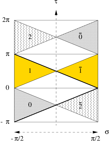
Figure 2: Subspaces of $\widehat{\rm AdS}_{2}$. The patch covered by the Poincaré coordinates $(t,r)$ is the bold bounded triangle; the wedges $W_{k}$ and $W_{\bar{k}}$, $k=0,1,2,\ldots$, are CPT conjugate to each other.

There is a unique wedge $W_{1}$ which together with its CPT conjugate lies in the primitive domain. It is characterized by the condition $t\pm r=\tan\frac{1}{2}(\tau\pm\sigma\pm\pi/2)\geq 0$, and thus in Poincaré coordinates is the cone $t\geq r\geq 0$. A convenient set of coordinates on $W_{1}$ is $(\xi,\rho),\,\xi\in\mbox{\rm IR},\,\rho\geq 0$, related to $(t,r)$ by $t=e^{\xi}{\rm ch}\rho,\,r=e^{\xi}{\rm sh}\rho$. Denoting by $\Phi(\xi,\rho)$ the field $\Phi(t,r)|_{W_{1}}$ in these coordinates one can use (22) to identify $H/2$ as the Hamiltonian for the cone, i.e.

$$e^{isH}\Phi(\xi,\rho)e^{-isH}=\Phi(\xi+2s,\rho)\,,\quad s\in\mbox{\rm IR}\;.$$ (42)

Let us write $W(\xi_{1}-\xi_{2};\rho_{1},\rho_{2})$ for the two-point function $W(t_{1}-t_{2};r_{1},r_{2})$ restricted to the cone $W_{1}$, where $(t_{i},r_{i})=(e^{\xi_{i}}{\rm ch}\rho_{i},e^{\xi_{i}}{\rm sh}\rho_{i})$, $i=1,2$. It enjoys the following Kubo-Martin-Schwinger property, which results in a thermalization phenomenon akin to the Unruh effect: As a function of $\xi_{1}-\xi_{2}$ $W$ is analytic in the strip $-2\pi<{\rm Im}(\xi_{1}-\xi_{2})<0$. The boundary values at the lower and upper rim of the strip are related by

$$W(\xi_{1}-\xi_{2}-2i\pi+i{\epsilon};\rho_{1},\rho_{2})=W(\xi_{2}-\xi_{1}-i{\epsilon};\rho_{2},\rho_{1})\;.$$ (43)

The proof is based on the primitive tubes of analyticity in [5] and the above CPT theorem; we omit the details. Let us emphasize that the result holds both for spacelike and timelike separated points $(t_{1},r_{1}),\,(t_{2},r_{2})\in W_{1}$; it does not refer to the worldlines of “observers” but is a property of the cone $W_{1}$: Restricting the quantum theory of the ER-scalar to $t\geq r\geq 0$, the Fock vacuum is a thermal state for the dilatation-evolution (42), with temperature $1/2\pi$. From the 4D viewpoint the restricted theory can be regarded as the quantum theory of those “exotic” ER-waves whose scalar $\phi(t,r)$ has support in $W_{1}$ only. The latter can be constructed explicitly by solving the wave eq. (4) in the $(\xi,\rho)$ coordinates. The ground state for $H$ however is not $SL(2,\mbox{\rm IR})$ invariant [4]. In the context of the ER-system the above thermal representation of the canonical commutation relations is therefore preferred in that it preserves more of the classical symmetries.

Boundary holography: In global coordinates the $r=0$ axis corresponds to the $\sigma=-\pi/2$ boundary of ${\rm AdS}_{2}$. Parallel to (26) we wish to reconstruct the field $\phi(\tau,\sigma)$ from its $\sigma=-\pi/2$ boundary values. Since $\phi(\tau,\sigma)$ is $2\pi$ anti-periodic in $\tau$ one can restrict attention to the primitive domain $-\pi<\tau<\pi$. It is convenient to introduce the mode sums

$$\!\!a^{-}({\theta})=\sum_{n\geq 0}a_{n}(-)^{n}e^{-i(n+1/2){\theta}},\;\;{\rm Im}\,{\theta}<0\;,\quad a^{+}({\theta})=\sum_{n\geq 0}a^{\dagger}_{n}(-)^{n}e^{i(n+1/2){\theta}},\;\;{\rm Im}\,{\theta}>0\,,$$ (44)

both declared to vanish in the other half-plane. They are $SU(1,1)$ densities of weight $1/2$, i.e.

$$U(g)a^{\pm}({\theta})U(g)^{-1}=\frac{a^{\pm}({\theta}^{g})}{|\beta e^{i{\theta}}+\alpha|}\;.$$ (45)

In terms of them we define the boundary field $\phi^{b}(\tau)$ by

$$\phi^{b}(\tau)=\cos\frac{\tau}{2}\lim_{{\epsilon}\rightarrow 0}\,[a^{+}(\tau+i{\epsilon})+a^{-}(\tau-i{\epsilon})]\;.$$ (46)

Classically the $a^{\pm}({\theta})$ play the role of scattering data wrt the $\tau$ evolution. One can recover them from a given $\phi^{b}(\tau)$ by factorizing it into a sum of functions $\cos\frac{{\theta}}{2}a^{\pm}({\theta})$ holomorphic in the upper and the lower half plane, respectively. The factorization has a unique solution in the primitive domain given by

$$\frac{1}{2\pi}\int_{-\pi}^{\pi}d\tau\frac{\phi^{b}(\tau)}{1-e^{-i(\tau-{\theta}-i{\epsilon})}}=\cos\frac{{\theta}}{2}\,a^{-}({\theta}-i{\epsilon})+\frac{1}{2}a_{0}^{\dagger}\;,$$ (47)

together with its hermitian conjugate yielding $a^{+}({\theta})$. The zero modes are easily split off and the classical reconstruction is completed by insertion of $a^{\pm}({\theta})$ into

$$\phi(\tau,\sigma) = \frac{1}{2\pi}\int_{-\pi}^{\pi}d{\theta}\,[a^{-}({\theta})\,\phi_{{\theta}}(\tau,\sigma)+a^{+}({\theta})\,\phi_{{\theta}}(\tau,\sigma)^{*}]\;,$$ (48)

$$\phi_{{\theta}}(\tau,\sigma) = \frac{1}{\sqrt{2}}\frac{(\cos\tau-\sin\sigma)^{1/2}\;e^{i({\theta}-\tau)/2}}{[1+2\sin\sigma e^{i({\theta}-\tau+i{\epsilon})}+e^{2i({\theta}-\tau+i{\epsilon})}]^{1/2}}\;,\quad{\epsilon}>0\;,$$ (49)

where $-\pi<\tau,{\theta}<\pi$. Since all transformations are linear the above procedure carries over to the quantum case when recast in terms of generic matrix elements of $\phi$. The $SU(1,1)$-covariance of the data $\phi^{b}(\tau)$, i.e. (37) at $\sigma=-\pi/2$, implies (37) for the reconstructed field operator.

References

• [1] K.ย Kuchar, Phys. Rev. D30 (1971) 955.
• [2] A.ย Ashtekar and M.ย Pierri, J. Math. Phys. 37 (1996) 6250; [gr-qc/9606085].
• [3] A.ย Ashtekar, Phys.ย Rev.ย Lett. 77 (1996) 4864; [gr-qc/9610008].
• [4] M.ย Spradlin and A.ย Strominger, JHEP 9909 (1999) 029; [hep-th/9904143].
• [5] M.ย Bertola, J.ย Bros, U.ย Moschella and R.ย Schaeffer, AdS/CFT correspondence for n-point functions, [hep-th/9908140].
• [6] M.ย Lรผscher and G.ย Mack, Comm.ย Math.ย Phys.ย 41 (1975) 203.
• [7] T.ย Nakatsu and N.ย Yokoi, Mod.ย Phys.ย Lett.ย A14 (1999) 147; [hep-th/9812047].
• [8] J.ย Swieca, Goldstoneโ€™s theorem and related topics, in: Cargese lectures, 1969, Vol 4.
• [9] S.ย Coleman, Commun. Math. Phys. 31 (1973) 259.
• [10] N.ย Vilenkin and A.ย Klimyk, Representations of Lie groups and special functions, Vol 1, Kluwer, 1991.
• [11] A.ย Ashtekar and M.ย Varadarajan, Phys.ย Rev.D50 (1994) 4944.
• [12] P.ย Breitenlohner and D.ย Maison, Ann. Inst, H. Poincarรฉ Phys. Thรฉor. 46 (1987) 215.
H.ย Nicolai, in: Recent aspects of quantum fields, ed.ย H.ย Mitter, Schladming, 1991.
• [13] M.ย Niedermaier and H.ย Samtleben, Nucl.ย Phys.ย B579 (2000) 437; [hep-th/9912111].