Maxwell stress tensor and the Casimir effect

Abstract

We evaluate the quantum correlators associated with the Maxwell field vacuum distorted by the presence of plane parallel material surfaces. Regularization is performed through the generalized zeta funtion technique. Results are applied to a local analysis of the atractive and repulsive Casimir effect through Maxwell stress tensor. Surface divergences are shown to cancel out when stresses on both sides of the material surface are taken into account. Since an atom can be considered as a probe of the local distortion of the quantum vacuum, Casimir-Polder interactions between atoms and material surfaces are also considered.

PACS: 11. 10. -z; 12. 20. -m

^† e-mail: farina@if.ufrj.br

^‡ e-mail:tort@if.ufrj.br

1 Introduction

According to Casimir [1], the (macroscopically) observable vacuum energy of a quantum field is the regularized difference between the zero point energies with and without the external conditions demanded by the particular physical situation at hand. In the case of the quantized electromagnetic field confined between two infinite parallel conducting plates separated by a distance $a$, Casimir’s conception of the vacuum energy leads to a force per unit area between the plates given by

$$\frac{F}{A}=-\frac{\pi\hbar c}{240\,a^{4}}.$$ (1)

Until 1997 only one experiment involving Casimir’s original setup had been performed [2]. Recently, however, the experimental observation of this tiny force with metallic surfaces was significantly improved by the experiments due to Lamoreaux and to Mohideen and Roy [3].The concept of an observable vacuum energy can be extended to all quantum fields and several types of boundary conditions and/or applied external fields. A review of all these Casimir effects can be found in, for example, Mostepanenko and Trunov or in Plunien et al. [4].

The local approach to the electromagnetic Casimir effect was initiated by Brown and Maclay who calculated the renormalized stress energy tensor between two parallel perfectly conducting plates by means of Green functions techniques [5]. An interesting approach to the standard Casimir effect is the one due to Gonzales [6]. This author pointed out that the apparently non-objectionable definition of the vacuum energy given above could easily lead to conceptual errors and stressed the fact that in any Casimir interaction calculation, contributions from both sides of the material surfaces involved must be taken into account. This is so because the vacuum pressure always pushes the material surfaces involved, therefore, the repulsiveness or atractiveness of the Casimir force depends on the discontinuity of the relevant component of the quantized Maxwell stress tensor at the location of the surface.

The purpose of this paper is to pursue this line of reasoning by analyzing the stresses on parallel material surfaces due to the vacuum distortions caused by the presence of these surfaces through the quantized Maxwell stress tensor. Though the approach chosen here has many points in common with Ref. [6] cited above, it is a different alternative in the sense that it relies on objects known as correlators, which are vacuum expectation values of products of field components taken at the same point in space and time. These correlators contain all the information we need on the local behavior of the vacuum expectation values of elements of Maxwell stress tensor, in particular, their behavior near both sides of the material surface in question, a feature crucial to the obtention of the correct result. The local behavior of the Maxwell tensor, or of the relativistic symmetrical stress-energy tensor, is extremely important because as shown by, for example, Deutsch and Candelas [11] with the help of Green functions technique, as we approach the boundaries we find strong divergencies that cannot be removed by renormalization. Besides reviewing the obtention of the electromagnetic Casimir for the standard case of two perfectly conducting parallel plates, we will also consider a pair of parallel plates, one of them perfectly permeable. This setup was first proposed by Boyer [7] who analyzed them from the viewpoint of random electrodymanics and it is the simplest example of a repulsive Casimir force. For both cases,  the conducting plate and Boyer’s setup we also construct the symmetrical stress tensor.

It is well-known that an atom can be attracted or repelled by a material surface, thus probing locally the vacuum distortions, for these reasons we take advantage of the knowledge of the above correlators and include a derivation of the Casimir-Polder interaction between an atom and a material surface. We will employ gaussian units and set $c=\hbar=1$.

2 Maxwell stress tensor and the electromagnetic field correlators

Our aim in this section is to obtain an expression for the quantum version of the electromagnetic force per unit area that acts on plane material surface. Material surface here means a perfectly conducting square surface($\epsilon\rightarrow\infty$) or a perfectly permeable one ($\mu\rightarrow\infty)$ whose linear dimension $L$ is much larger than others relevant dimensions envolved such as the distance between two of those surfaces. The physical interaction between any of the two types of surfaces considered here and the vacuum electromagnetic field is mimicked by the imposition of appropriate boundary conditions on the electromagnetic field on the location of the material surface. The Cartesian components of the Maxwell stress tensor in Gaussian units are given by [8]

$$T_{ij}=\frac{1}{4\pi}\left(E_{i}\,E_{j}-\frac{1}{2}\,\delta_{ij}\mathbf{E}^{2}+B_{i}\,B_{j}-\frac{1}{2}\,\delta_{ij}\mathbf{B}^{2}\right)$$ (2)

where $i,j=x,y,z$. Suppose that the material surface is placed perpendicularly to the $\mathcal{OZ}$ axis. Upon quantizing the electromagnetic field we can write the quantum version of (2). For instance,

$$\left\langle\hat{T}_{zz}\right\rangle_{0}=\frac{1}{8\pi}\left[\left\langle\hat{E}_{z}^{2}\right\rangle_{0}-\left\langle\hat{E}_{\parallel}^{2}\right\rangle_{0}+\left\langle\hat{B}_{z}^{2}\right\rangle_{0}-\left\langle\hat{B}_{\parallel}^{2}\right\rangle_{0}\right],$$ (3)

where $\hat{E}_{\parallel}^{2}=\hat{E}_{x}^{2}+\hat{E}_{y}^{2}$ and $\hat{B}_{\parallel}^{2}=\hat{B}_{x}^{2}+\hat{B}_{y}^{2}$; $\left\langle\hat{O}\right\rangle_{0}\equiv\left\langle 0\right|\hat{O}\left|0\right\rangle$ denotes a vacuum expectation value. The other Cartesian components of this tensor can be obtained in an analogous way. The quantum macroscopic force$\left\langle\mathbf{\hat{F}}\right\rangle_{0}$ on the material surface can be evaluated by integrating the quantum version of the classical result[8]

$$\mathbf{F=}\oint_{\partial\mathcal{R}}\mathbf{\tilde{T}\cdot\hat{n}}\,da,$$ (4)

were $\mathbf{\hat{n}}$ is outwards normal at $\partial\mathcal{R}$ and $\mathcal{R}$ is any region containing the material surface. Classically, (4) can be obtained by integrating the Lorentz force per unit volume acting on charge and current distributions and eliminating the sources in favor of the fields. From a quantum point of view, we see that the problem of evaluating the pressure the material surface due to the distorted zero point oscillations of the electromagnetic field is reduced to the evaluation of the vacuum expectation value of the quantum operators $\hat{E}_{i}\left(\mathbf{r},t\right)\hat{E}_{j}\left(\mathbf{r},t\right)$, $\hat{B}_{i}\left(\mathbf{r},t\right)\hat{B}_{j}\left(\mathbf{r},t\right),$ and $\hat{E}_{i}\left(\mathbf{r},t\right)\hat{B}_{j}\left(\mathbf{r},t\right)$. The evaluation of these correlators depends on the specific choice of the boundary conditions. A regularization recipe will also be necessary, for these objects are mathematically ill-defined. For the setup envolving conducting plates these correlators were evaluated by Lütken and Ravndal [14], see also [9]. They can be also obtained from the coincidence limit of the photon propagator between conducting plates evaluated by Bordag et al [15]. In the next section we will display a method of evaluating these correlators by means of analitycal continuation techniques [10] similar to the ones employed by Lütken e Ravndal [14]. We will also show how to obtain the corresponding results for another unusual but intersting setup [10].

3 Correlators for Casimir’s setup

Consider an experimental setup consisting in two infinite perfectly conducting parallel plates ($\epsilon\rightarrow\infty$) kept at a fixed distance $a$ from each other. We will choose the coordinates axis in such a way that the $\mathcal{OZ}$ direction is perpendicular to the plates. One of the plates will be placed at $z=0$ and the othrt one at $z=a$. The field must satisfy the following boundary conditions on the plates: the tangential components $E_{x}$ e $E_{y}$ of the electric field and the normal component $B_{z}$ of the magnetic field must be zero on the plates. Since there are no real charges or currents it will be convenient to work in the Coulomb gauge in which $\mathbf{\nabla}\cdot\mathbf{A}(\mathbf{r},t)=0$, and $\Phi=0$, thus $\mathbf{E}(\mathbf{r},t)=-\partial\mathbf{A}(\mathbf{r},t)/\partial t$ and $\mathbf{B}(\mathbf{r},t)=\mathbf{\nabla}\times\mathbf{A}\left(\mathbf{r,t}\right)$. These physical boundary conditions combined with the choice of gauge allow us to rewrite the boundary conditions in terms of the components of the vector potential $\mathbf{A}(\mathbf{r},t)$ in the following way: at $\ z=0$ we will have,

$$A_{x}(x,y,0,t)=0\,;\;\;\;\;A_{y}(x,y,0,t)=0\,;\;\;\;\;{\frac{\partial}{\partial z}}A_{z}(x,y,0,t)=0\,,$$ (5)

and at $z=a$ ,

$$A_{x}(x,y,a,t)=0\,;\;\;\;\;A_{y}(x,y,a,t)=0\,;\;\;\;\;{\frac{\partial}{\partial z}}A_{z}(x,y,a,t)=0\,\,.$$ (6)

The vector potential operator $\mathbf{\hat{A}}(\mathbf{r},t)$ that satisfies the wave equation, the Coulmb gauge and the boundary conditions can be written as

$$\mathbf{\hat{A}}(\mathbf{r},t) = {\frac{1}{\pi}}\left({\frac{\pi}{a}}\right)^{\frac{1}{2}}\sum_{n=0}^{\;\;\infty\;\;\prime\prime}\int\,{\frac{d^{2}\mathbf{\kappa}}{\sqrt{\omega}}}\left\{\hat{a}^{(1)}(\mathbf{\kappa},n)\mathbf{\hat{\kappa}}\times\hat{\mathbf{z}}\sin\left({\frac{n\pi z}{a}}\right)\right.$$ (7)

$$+ \left.\hat{a}^{(2)}(\mathbf{\kappa},n)\left[\mathbf{\hat{\kappa}}{\frac{in}{\omega a}}\sin\left({\frac{n\pi z}{a}}\right)-\mathbf{\hat{z}}{\frac{\kappa}{\omega}}\cos\left({\frac{n\pi z}{a}}\right)\right]\right\}e^{i(\mathbf{\kappa}\cdot\mathbf{\rho}-\omega t)}\;+h.c,$$

where $\mathbf{\kappa}=(k_{x},k_{y})$ and $\mathbf{\rho}$ is the position arrow on the $\mathcal{XY}$ plane. The normal frquencies are given by

$$\omega=\omega(\mathbf{\kappa},n)=\sqrt{\mathbf{\kappa}^{2}+n^{2}{\frac{\pi^{2}}{a^{2}}}},$$ (8)

with $k_{x},k_{y}\in\mathbb{R}$ e $n\in\mathbb{N-}1$. The symbol $\sum^{"}$ indicates that the term corresponding to $n=0$ for normaliztion reasons must be multiplied by $1/2$ . The Fourier coefficients $\hat{a}^{(\lambda)}(\mathbf{\kappa},n)$ where $\lambda=1,2$ is  the polarization index, are operators  in the photon ocupation number space and satisfy

$$\left[\hat{a}^{(\lambda)}(\mathbf{\kappa},n),\hat{a}^{\dagger(\lambda^{\prime})}(\mathbf{\kappa}^{\prime},n^{\prime})\right]=\delta_{\lambda\lambda^{\prime}}\delta_{nn^{\prime}}\delta\left(\mathbf{\kappa}-\mathbf{\kappa}^{\prime}\right)\,.$$ (9)

It is convenient to write the vector potential in the general form

$$\mathbf{\hat{A}}(\mathbf{r},t)=\sum_{n=0}^{\;\;\infty\;\;\prime\prime}\int\,{d^{2}}\mathbf{\kappa}\sum_{\lambda=1}^{2}\hat{a}^{(\lambda)}(\mathbf{\kappa},n)\mathbf{A}_{\mathbf{\kappa}n}^{(\lambda)}(\mathbf{r})e^{-i\omega(\mathbf{\kappa},n)t}+h.c\,,$$ (10)

where $\mathbf{A}_{\mathbf{\kappa}n}^{(\lambda)}(\mathbf{r})$ are the modal functions. The modal functions for each polarization state must obey Helmholtz equation and the boundary conditions given above. In our case the modal functions are

$$\mathbf{A}_{\mathbf{\kappa\,}n}^{(1)}(\mathbf{r})={\frac{1}{\pi}}\left({\frac{\pi}{a}}\right)^{\frac{1}{2}}{\frac{1}{\sqrt{\omega}}}\sin\left({\frac{n\pi z}{a}}\right)e^{-i\mathbf{\kappa}\cdot\mathbf{\rho}}\,\mathbf{\hat{\kappa}}\times\mathbf{\hat{z}}\,,$$ (11)

and

$$\mathbf{A}_{\mathbf{\kappa\,}n}^{(2)}(\mathbf{r})={\frac{1}{\pi}}\left({\frac{\pi}{a}}\right)^{\frac{1}{2}}{\frac{1}{\sqrt{\omega}}}\left[\mathbf{\hat{\kappa}}{\frac{in\pi}{a\omega}}\sin\left({\frac{n\pi z}{a}}\right)-\mathbf{\hat{z}}{\frac{\kappa}{\omega}}\cos\left({\frac{n\pi z}{a}}\right)\right]e^{-i\mathbf{\kappa}\cdot\mathbf{\rho}}\,.$$ (12)

The next step is to evaluate the electric field operator $\mathbf{\hat{E}}(\mathbf{r},t)$. Recalling that $\hat{a}^{(\lambda)}(\mathbf{\kappa},n)|0\rangle=0,$ we first write the correlators $<\hat{E}_{i}(\mathbf{r},t)\hat{E}_{j}(\mathbf{r},t)\rangle_{0}$ in the general form

$$<\hat{E}_{i}(\mathbf{r},t)\hat{E}_{j}(\mathbf{r},t)\rangle_{0}=\sum_{\alpha}E_{i\alpha}(\mathbf{r})E_{j\alpha}^{\ast}(\mathbf{r})\,,$$ (13)

where we have introduced the modal functions $E_{i\alpha}(\mathbf{r})$ for the electric field. In our case (11) and (12) yield

$$\mathbf{E}_{i\,\mathbf{\kappa}\,n}^{(1)}(\mathbf{r})={\frac{i}{\pi}}\left({\frac{\omega\left(\mathbf{\kappa,}n\right)\pi}{a}}\right)^{\frac{1}{2}}\,\sin\left({\frac{n\pi z}{a}}\right)e^{-i\mathbf{\kappa}\cdot\mathbf{\rho}}\,(\mathbf{\hat{\kappa}}\times\mathbf{\hat{z}})_{i}\,,$$ (14)

and,

$$\mathbf{E}_{i\,\mathbf{\kappa\,}n}^{(2)}(\mathbf{r})={\frac{i}{\pi}}\left({\frac{\omega\left(\mathbf{\kappa,}n\right)\pi}{a}}\right)^{\frac{1}{2}}\,\left[\mathbf{\kappa}_{i}{\frac{in\pi}{a\,\omega\left(\mathbf{\kappa,}n\right)}}\sin\left(\frac{n\pi z}{a}\right)-\mathbf{\hat{z}}_{i}{\frac{\kappa}{\omega\left(\mathbf{\kappa,}n\right)}}\cos\left(\frac{n\pi z}{a}\right)\right]e^{-i\mathbf{\kappa}\cdot\mathbf{\rho}}\,,$$ (15)

respectively. Taking (14) and (15) into (13), we write $\mathbf{\hat{\kappa}}_{i}=\cos\phi\,\delta_{ix}+\sin\phi\,\delta_{iy}$, $\mathbf{\hat{z}}_{i}=\delta_{iz}$ e $(\mathbf{\hat{z}}\times\mathbf{\hat{\kappa}})_{i}=\sin\phi\,\delta_{ix}-\cos\phi\,\delta_{iy}$, where $\phi$ is the azimuthal angle on the $\mathcal{XY}$ plane and we have performed all angular integrals. In this way we end up with

$$\langle{\hat{E}}_{i}(\mathbf{r},t){\hat{E}}_{j}(\mathbf{r},t)\rangle_{0}\;\;=\;\;\left({\frac{2}{\pi}}\right)\left({\frac{\pi}{a}}\right){\frac{\delta_{ij}^{\|}}{2}}\sum_{n=0}^{\;\;\infty\;\;\prime\prime}\sin^{2}\left(\frac{n\pi z}{a}\right)\int_{0}^{\infty}d\kappa\,\kappa\,\omega(\mathbf{\kappa},n)$$ (16)

$$+ \left({\frac{2}{\pi}}\right)\left({\frac{\pi}{a}}\right)\left({\frac{\pi}{a}}\right)^{2}{\frac{\delta_{ij}^{\|}}{2}}\sum_{n=0}^{\;\;\infty\;\;\prime\prime}n^{2}\sin^{2}\left(\frac{n\pi z}{a}\right)\int_{0}^{\infty}d\kappa\,\kappa\,\omega^{-1}(\mathbf{\kappa},n)$$

$$+ \left({\frac{2}{\pi}}\right)\left({\frac{\pi}{a}}\right)\delta_{ij}^{\bot}\sum_{n=0}^{\;\;\infty\;\;\prime\prime}\cos^{2}\left(\frac{n\pi z}{a}\right)\int_{0}^{\infty}d\kappa\,\kappa^{3}\,\omega^{-1}(\mathbf{\kappa},n)\,,$$

where $\delta_{ij}^{\|}:=\delta_{ix}\delta_{jx}+\delta_{iy}\delta_{jy}$ e $\delta_{ij}^{\bot}:=\delta_{iz}\delta_{jz}$. Equation (16) is a formal expression for the correlator $\langle E_{i}(\mathbf{r},t)E_{j}(\mathbf{r},t)\rangle_{0}$, since it is mathematically ill-defined unless a regularization recipe is prescribed. We will regularize the integrals in (16) with the help of analytical continuation methods.

Consider, for instance, the first integral on the r.h.s. of (16) and let us rewrite it as follows

$$\int_{0}^{\infty}d\kappa\kappa\left(\kappa^{2}+{\frac{n^{2}\pi^{2}}{a^{2}}}\right)^{1/2}\rightarrow\int_{0}^{\infty}d\kappa\kappa\left(\kappa^{2}+{\frac{n^{2}\pi^{2}}{a^{2}}}\right)^{1/2-s}.\;$$

The first term in (16) can be rewritten as

$$T_{1}=\left({\frac{2}{\pi}}\right)\left({\frac{\pi}{a}}\right){\frac{\delta_{ij}^{\|}}{2}}\sum_{n=0}^{\infty"}\sin^{2}\left(\frac{n\pi z}{a}\right)\int_{0}^{\infty}d\kappa\,\kappa\,\left(\mathbf{\kappa}^{2}+\frac{n^{2}\pi^{2}}{a^{2}}\right)^{-\frac{1}{2}-s},$$ (17)

the second as

$$T_{2}=\left({\frac{2}{\pi}}\right)\left({\frac{\pi}{a}}\right)\left({\frac{\pi}{a}}\right)^{2}{\frac{\delta_{ij}^{\|}}{2}}\sum_{n=0}^{\infty"}n^{2}\sin^{2}\left(\frac{n\pi z}{a}\right)\int_{0}^{\infty}d\kappa\,\kappa\left(\mathbf{\kappa}^{2}+\frac{n^{2}\pi^{2}}{a^{2}}\right)^{-\frac{1}{2}-s},$$ (18)

and the third one as

$$T_{3}=\left({\frac{2}{\pi}}\right)\left({\frac{\pi}{a}}\right)\delta_{ij}^{\bot}\sum_{n=0}^{\infty"}\cos^{2}\left(\frac{n\pi z}{a}\right)\int_{0}^{\infty}d\kappa\,\kappa^{3}\,\left(\mathbf{\kappa}^{2}+\frac{n^{2}\pi^{2}}{a^{2}}\right)^{-\frac{1}{2}-s}.$$ (19)

Let us assume that $\Re\,s$ is large enough to give precise mathematical meaning to these integrals. After evaluating them and make use of the analytical continuation of the results we will take the limit $s\rightarrow 0$. Let us see, for instance, what happens with $T_{1}$. Making use of the following representation of Euler beta function [17]

$$\int_{0}^{\infty}dx\,x^{\mu-1}\left(x^{2}+c^{2}\right)^{\nu-1}={\frac{B}{2}}\left({\frac{\mu}{2}},1-\nu-{\frac{\mu}{2}}\right)c^{\mu+2\nu-2}\,,$$ (20)

where $B(x,y)=\Gamma(x)\Gamma(y)/\Gamma(x+y)$, and that holds for $\Re\,\left(\nu+{\frac{\mu}{2}}\right)<1$ and $\Re\,\mu>0$, we obtain

$$\int_{0}^{\infty}d\kappa\kappa\left(\kappa^{2}+{\frac{n^{2}\pi^{2}}{a^{2}}}\right)^{1/2-s}={\frac{1}{2}}\left({\frac{n\pi}{a}}\right)^{3-2s}\;{\frac{\Gamma(s-3/2)}{\Gamma(s-1/2)}}={\frac{1}{(2s-3)}}\left({\frac{n\pi}{a}}\right)^{3-2s}\;.$$ (21)

Taking this result into $T_{1}$ we obtain

$$T_{1}=\left({\frac{1}{2s-3}}\right)\left({\frac{\pi}{a}}\right)^{3-2s}{\frac{\delta_{ij}^{\|}}{2a}}\left[\zeta_{R}(2s-3)-\sum_{n=0}^{\infty}n^{3-2s}\cos\left({\frac{2n\pi z}{a}}\right)\right]\;,$$ (22)

where $\zeta_{R}(z)$ is the well-known Riemann zeta function. Taking the limit $s\rightarrow 0$, we have

$$T_{1}=-{\frac{1}{3\pi}}\left({\frac{\pi}{a}}\right)^{4}\frac{\delta_{ij}^{\|}}{2}\left[{\frac{1}{120}}+\frac{1}{8}\sum_{n=1}^{\infty}\frac{d^{3}}{d{\xi}^{{3}}}\sin\left(2n\xi\right)\right]\;,$$ (23)

where we made use of the fact that $\zeta_{R}(-3)=1/120$, defined $\xi:=\pi z/a$, and wrote

$$n^{3}\cos\left(2n\xi\right)=-\frac{1}{8}\times{\frac{d^{3}}{d\xi^{3}}\sin}\left(2n\xi\right).$$ (24)

The sum on the R.H.S. of (23) can be regularized in many ways. A quick though non-rigorous way is to write

$$T_{1}=-{\frac{1}{3\pi}}\left({\frac{\pi}{a}}\right)^{4}\frac{\delta_{ij}^{\|}}{2}\left[{\frac{1}{120}}+\frac{1}{8}\frac{d^{3}}{d{\xi}^{{3}}}\sum_{n=1}^{\infty}\sin\left(2n\xi\right)\right],\;$$ (25)

and express the summand in terms of exponential functions of imaginary argument thereby transforming each one of the sums into the euclidean space. In this way we obtain

$$\sum_{n=1}^{\infty}\sin\left(2n\xi\right) = \frac{1}{2i}\left(\sum_{n=1}^{\infty}\exp\left(i2n\xi\right)-\sum_{n=1}^{\infty}\exp\left(-i2n\xi\right)\right)$$ (26)

$$= \frac{1}{2i}\left(\sum_{n=1}^{\infty}\exp\left(2n\xi_{E}\right)-\sum_{n=1}^{\infty}\exp\left(-2n\xi_{E}^{\prime}\right)\right)$$

where we have made the substitution $i\xi\to-\xi_{E}$ in the first sum and $i\xi\to\xi_{E}^{\prime}$ in the second. Each one of the sums above can be easily performed and the result is

$$\sum_{n=1}^{\infty}\sin\left(2n\xi\right)=\frac{1}{2}\cot\left(\xi\right)$$ (27)

It follows that

$$T_{1}=-{\frac{1}{3\pi}}\left({\frac{\pi}{a}}\right)^{4}\frac{\delta_{ij}^{\|}}{2}\left[{\frac{1}{120}}+\frac{1}{8}\frac{d^{3}}{d{\xi}^{{3}}}\frac{1}{2}\cot\left(\xi\right)\right].$$ (28)

Treating the two other terms in (16) in a similar manner we obtain

$$T_{2}=-{\frac{1}{\pi}}\left({\frac{\pi}{a}}\right)^{4}\frac{\delta_{ij}^{\|}}{2}\left[{\frac{1}{120}}+\frac{1}{8}\frac{d^{3}}{d{\xi}^{{3}}}\frac{1}{2}\cot\left(\xi\right)\right],$$ (29)

and

$$T_{3}={\frac{4}{3\pi}}\left({\frac{\pi}{a}}\right)^{4}\frac{\delta_{ij}^{\bot}}{2}\left[{\frac{1}{120}}-\frac{1}{8}\frac{d^{3}}{d{\xi}^{{3}}}\frac{1}{2}\cot\left(\xi\right)\right].$$ (30)

Notice that some care must be taken when we aply this procedure to the third term. This is so because the term corresponding to $n=0$ in $T_{3}$ is not zero. In fact its contribution is:

$$T_{3}(n=0)=\left({\frac{2}{\pi}}\right)\left({\frac{\pi}{a}}\right)\delta_{ij}^{\bot}\int_{0}^{\infty}d\kappa\,\kappa\,^{-2-2s},$$ (31)

which diverges when the regularization is removed. How ever this term is non-physical and can be safely ignored. Finally, collecting all partial results we have

$$\langle E_{i}(\mathbf{r},t)E_{j}(\mathbf{r},t)\rangle_{0} = T_{1}+T_{2}+T_{3}$$ (32)

$$= \left({\frac{\pi}{a}}\right)^{4}{\frac{2}{3\pi}}\left[\left(-\delta^{\|}+\delta^{\bot}\right)_{ij}\;{\frac{1}{120}}+\delta_{ij}F(\xi)\right]\,.$$

The function $\,F\left(\xi\right)$ is defined by

$$F\left(\xi\right):=-\frac{1}{8}\frac{d^{3}\,}{d\xi^{3}}\frac{1}{2}\cot\left(\xi\right),$$ (33)

and its expansion about $\xi=0$ is given by

$$F\left(\xi\right)\approx\frac{3}{8}\xi^{-4}+\frac{1}{120}+O\left(\xi^{2}\right).$$ (34)

Near $\xi=\pi$ (which corresponds to $z=a$) we make the replacement $\xi\rightarrow\xi-\pi$. Notice that due to the behavior of $F\left(\xi\right)$ near $\xi=0,a$, strong divergences predominate in the behavior of the correlators near the plates.

By applying the exactly the same procedure we obtain the magnetic field correlators

$$\langle B_{i}(\mathbf{r},t)B_{j}(\mathbf{r},t)\rangle_{0}=\left({\frac{\pi}{a}}\right)^{4}{\frac{2}{3\pi}}\left[\left(-\delta^{\|}+\delta^{\bot}\right)_{ij}\;{\frac{1}{120}}-\delta_{ij}F(\xi)\right]\,.$$ (35)

A direct evaluation also shows that the correlators $<E_{i}(\mathbf{r},t)B_{j}(\mathbf{r},t)\rangle_{0}$ are zero.

4 Correlators for Boyer’s setup

The other setup we are interested in is that one in which a perfectly conducting plate is placed at $z=0$ and perfectly permeable plate is placed at $z=a$. This setup was analyzed for the first time by Boyer in the contetxt of stochastic electrodynamic [7] and it is the simplest case of a repulsive Casimir effect that can be found in the literature. The boundary conditions now are: (a) the tangential components $E_{x}$ and $E_{y}$ of the electric field as well as the normal component $B_{z}$ of the magnetic field must vanish on the surface of the plate at $z=0$; (b) the tangential components of $B_{x}$ e $B_{y}$ of the magnetic field as well as normal conponent $E_{z}$ of the electric field must vanish on the surface of the plate at $z=a$. These boundary conditions translated in terms of the components of the vector potential read

$$A_{x}(x,y,0,t)=0\,;\;\;\;\;A_{y}(x,y,0,t)=0\,;\;\;\;\;{\frac{\partial}{\partial z}}A_{z}(x,y,0,t)=0\,,$$ (36)

at $\ z=0$, and at $z=a$

$${\frac{\partial}{\partial x}}A_{x}(x,y,a,t)=0\,;\;\;\;\;{\frac{\partial}{\partial y}}A_{y}(x,y,a,t)=0\,;\;\;\;\;A_{z}(x,y,a,t)=0\,.$$ (37)

The appropriate vector potential operator $\mathbf{\hat{A}}(\mathbf{r},t)$ is given by [10]

$$\mathbf{\hat{A}}(\mathbf{r},t) = {\frac{1}{\pi}}\left({\frac{\pi}{a}}\right)^{\frac{1}{2}}\sum_{n=0}^{\infty}\int\,{\frac{d^{2}\mathbf{\kappa}}{\sqrt{\omega}}}\left\{\hat{a}^{(1)}(\mathbf{\kappa},n)\mathbf{\hat{\kappa}}\times\hat{\mathbf{z}}\sin\left[\left(n+{\frac{1}{2}}\right){\frac{\pi z}{a}}\right]\right.$$ (38)

$$+ \left.\hat{a}^{(2)}(\mathbf{\kappa},n)\left[\mathbf{\hat{\kappa}}{\frac{i(n+{\frac{1}{2}})}{\omega a}}\sin\left[\left(n+{\frac{1}{2}}\right){\frac{\pi z}{a}}\right]-\mathbf{\hat{z}}{\frac{\kappa}{\omega}}\cos\left[\left(n+{\frac{1}{2}}\right){\frac{\pi z}{a}}\right]\right]\right\}$$

$$\times e^{i(\mathbf{\kappa}\cdot\mathbf{\rho}-\omega t)}\;+\text{ }h.c.,$$

where as before $\mathbf{\kappa}=(k_{x},k_{y})$ and $\mathbf{\rho}$ is the position vector on the $\mathcal{XY}$ plane. The normal frequencies are given

$$\omega(\mathbf{\kappa},n)=\sqrt{\mathbf{\kappa}^{2}+\left(n+{\frac{1}{2}}\right)^{2}{\frac{\pi^{2}}{a^{2}}}}\,,$$ (39)

with $k_{x},k_{y}\in\mathbb{R}$ and $n\in\mathbb{N-}1$. Notice that contrary to the case of two conducting plates normalization does not require the we multiply the term corresponding to $n=0$ by $1/2$. The electric and magnetic field correlators for Boyer’s setup can be evaluated with the same technique employed before [10]. In fact, it is not hard to convince ourselves that it is sufficient to perform the substitution $n\to n+1/2$  and follow the same steps as before to obtain

$$\langle E_{i}(\mathbf{r},t)E_{j}(\mathbf{r},t)\rangle_{0}=T_{1}+T_{2}+T_{3},$$ (40)

where, for example

$$T_{1}=\frac{\Gamma\left(s-\frac{3}{2}\right)}{\Gamma\left(s-\frac{1}{2}\right)}\left({\frac{\pi}{a}}\right)^{3-2s}{\frac{\delta_{ij}^{\|}}{2a}}\left\{\sum_{n=0}^{\infty}\left(n+\frac{1}{2}\right)^{3-2s}\frac{1}{2}\left[1-\cos\left(2\left(n+1/2\right)\frac{\pi z}{a}\right)\right]\right\},\;$$ (41)

The terms $T_{2}$ e $T_{1}$ show a similar structure. The main difference with respect to the two conducting plate case is that now we have to deal with the Hurwitz zeta function $\zeta_{H}(z,q)$ which has a series representation given by [17]

$$\zeta_{H}(z,q)=\sum_{n=0}^{\infty}\frac{1}{\left(n+q\right)^{z}},$$ (42)

with $\Re\,z>1$, and $q\neq 0,-1,-2,....$. In our case we must set

$$\zeta_{H}(2s-3,\frac{1}{2})=\sum_{n=0}^{\infty}\left(n+\frac{1}{2}\right)^{3-2s}.$$ (43)

It follows that in the limit $s\rightarrow 0$ we have

$$T_{1}=-\left({\frac{\pi}{a}}\right)^{4}\frac{1}{3\pi}{\frac{\delta_{ij}^{\|}}{2}}\left\{\zeta_{H}\left(-3,\frac{1}{2}\right)+\sum_{n=0}^{\infty}\left(n+\frac{1}{2}\right)^{3}\cos\left(2\left(n+\frac{1}{2}\right)\frac{\pi z}{a}\right)\right\}.$$ (44)

In the same way we obtain for $T_{2}$ e $T_{1}$ the results

$$T_{2}=-\left({\frac{\pi}{a}}\right)^{4}\frac{1}{\pi}{\frac{\delta_{ij}^{\|}}{2}}\left\{\zeta_{H}\left(-3,\frac{1}{2}\right)-\sum_{n=0}^{\infty}\left(n+\frac{1}{2}\right)^{3}\cos\left(2\left(n+\frac{1}{2}\right)\frac{\pi z}{a}\right)\right\}.$$ (45)

and

$$T_{3}=\left({\frac{\pi}{a}}\right)^{4}\frac{2}{3\pi}{\frac{\delta_{ij}^{\bot}}{2}}\left\{\zeta_{H}\left(-3,\frac{1}{2}\right)+\sum_{n=0}^{\infty}\left(n+\frac{1}{2}\right)^{3}\cos\left(2\left(n+\frac{1}{2}\right)\frac{\pi z}{a}\right)\right\}.$$ (46)

Notice that this time we do not have the divergent contribution corresponding to $n=0$ as in the case of the conducting plates. Adding the three terms we have

$$\left\langle\hat{E}_{i}\left(\mathbf{r},t\right)\hat{E}_{j}\left(\mathbf{r},t\right)\right\rangle_{0} = \left({\frac{\pi}{a}}\right)^{4}\frac{2}{3\pi}\left\{(-\delta_{ij}^{\|}+\delta_{ij}^{\bot})\zeta_{H}\left(-3,\frac{1}{2}\right)\right.$$ (47)

$$\left.+\sum_{n=0}^{\infty}\left(n+\frac{1}{2}\right)^{3}\cos\left(2\left(n+\frac{1}{2}\right)\frac{\pi z}{a}\right)\right\}.$$

The numerical value $\zeta_{H}\left(-3,\frac{1}{2}\right)$ can be obtained from [17]

$$\zeta_{H}\left(-n,q\right)=-\frac{B_{n+1}(q)}{n+1},$$ (48)

where $n\in\mathbf{N}$ and $B_{n+1}(q)$ is a Bernoulli polynomial defined by [17]

$$B_{n}(x)=\sum_{p=0}^{n}\frac{n!}{p!(n-p)!}B_{p}x^{n-k},$$ (49)

where $B_{p}$ is a Bernoulli number. The relevant polynomial here is:

$$B_{4}(x)=x^{4}-2x^{3}+x^{2}-\frac{1}{30}.$$ (50)

With $B_{4}(1/2)=(7/8)\times(1/30)$, it follows that $\zeta_{H}\left(-3,\frac{1}{2}\right)=-(7/8)(1/120)$. The sum can be regularized with the same technique employed before. In fact, we can define the function $G(\xi)$ by

$$G(\xi) : =\sum_{n=0}^{\infty}\left(n+\frac{1}{2}\right)^{3}\cos\left[2\left(n+\frac{1}{2}\right)\xi\right]$$ (51)

$$= \frac{1}{8}\sum_{n=0}^{\infty}\left(2n+1\right)^{3}\cos\left[\left(2n+1\right)\xi\right],$$

where as before $\xi:=z\pi/a$. We can write

$$\left(2n+1\right)^{3}\cos\left[\left(2n+1\right)\xi\right]=-\frac{d^{3}}{d\xi^{3}}\sin\left[\left(2n+1\right)\xi\right]$$ (52)

and formally we have

$$G(\xi)=-\frac{1}{8}\frac{d^{3}}{d\xi^{3}}\sum_{n=0}^{\infty}\sin\left[\left(2n+1\right)\xi\right].$$ (53)

Writing $\sin\left[\left(2n+1\right)\xi\right]$ in terms of exponentials of imaginary argument and passing to the euclidean space we obtain after some simple manipulations

$$\,G\left(\xi\right)=-\frac{1}{8}\frac{d^{3}\,}{d\xi^{3}}\frac{1}{2\sin\left(\xi\right)}.$$ (54)

Collecting all partial results we finally obtain for $\left\langle\hat{E}_{i}\left(\mathbf{r},t\right)\hat{E}_{j}\left(\mathbf{r},t\right)\right\rangle_{0}$ the result

$$\left\langle\hat{E}_{i}\left(\mathbf{r},t\right)\hat{E}_{j}\left(\mathbf{r},t\right)\right\rangle_{0}=\left(\frac{\pi}{a}\right)^{4}\frac{2}{3\pi}\left[\left(-\frac{7}{8}\right)\frac{\left(-\delta^{\|}+\delta^{\perp}\right)_{ij}}{120}+\delta_{ij}\,G\left(\xi\right)\right].$$ (55)

Proceeding in the same way in the evaluation of $\left\langle\hat{B}_{i}\left(\mathbf{r},t\right)\hat{B}_{j}\left(\mathbf{r},t\right)\right\rangle_{0}$ we obtain

$$\left\langle\hat{B}_{i}\left(\mathbf{r},t\right)\hat{B}_{j}\left(\mathbf{r},t\right)\right\rangle_{0}=\left(\frac{\pi}{a}\right)^{4}\frac{2}{3\pi}\left[\left(-\frac{7}{8}\right)\frac{\left(-\delta^{\|}+\delta^{\perp}\right)_{ij}}{120}-\delta_{ij}\,G\left(\xi\right)\right].$$ (56)

Observe that near $\xi=0$ the function $G\left(\xi\right)$ behaves as

$$G\left(\xi\right)=\frac{3}{8}\xi^{-4}-\frac{7}{8}\,\frac{1}{120}+O\left(\xi^{2}\right),$$ (57)

But near $\xi=\pi$ its behavior is slightly different

$$G\left(\xi\right)=-\frac{3}{8}\left(\xi-\pi\right)^{-4}+\frac{7}{8}\,\frac{1}{120}+O\left[\left(\xi-\pi\right)^{2}\right].$$ (58)

Again, a direct calculation shows that $\left\langle\hat{E}_{i}\left(\mathbf{r},t\right)\hat{B}_{j}\left(\mathbf{r},t\right)\right\rangle_{0}=0$ for this case.

As before the divergent behavior of the correlators near the plates we are interested in is an effect of the distortions of the electromagnetic oscillations with respect to a situation where the plates are not present. This fact has received the attention of several authors, see for example [11, 14].

5 The Casimir effect for conducting plates

In order to apply the above results to Casimir’s original setup we consider for convenience three parallel perfectly conducting plates perpendicular to the $\mathcal{OZ}$ axis at $z=0$, $z=a$ and $z=\ell$.

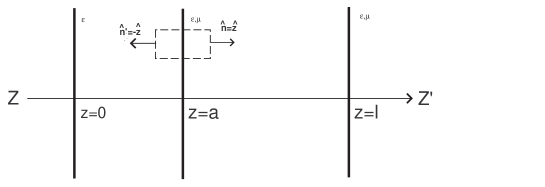
Figure 1: Three-plate setup for the obtention of the Casimir force per unit area. The plate at $z=\ell$ is auxiliary.

The quantum version of Maxwell tensor is

$$4\pi\left\langle\hat{T}_{ij}\right\rangle_{0}=\left\langle\hat{E}_{i}\,\hat{E}_{j}\right\rangle_{0}-\frac{1}{2}\,\delta_{ij}\left\langle\mathbf{\hat{E}}^{2}\right\rangle_{0}+\left\langle\hat{B}_{i}\,\hat{B}_{j}\right\rangle_{0}-\frac{1}{2}\,\delta_{ij}\left\langle\mathbf{\hat{B}}^{2}\right\rangle_{0}$$ (59)

Making use of the correlator given by (32) we obtain the following partial results

$$\left\langle\hat{E}_{x}^{2}(z,t)\right\rangle_{0}=\left\langle\hat{E}_{y}^{2}(z,t\right\rangle_{0}=\left(\frac{\pi}{a}\right)^{4}\frac{2}{3\pi}\left[-\frac{1}{120}+F\left(\xi\right)\right],$$ (60)

$$\left\langle\hat{E}_{z}^{2}(z,t\right\rangle_{0}=\left(\frac{\pi}{a}\right)^{4}\frac{2}{3\pi}\left[\frac{1}{120}+F\left(\xi\right)\right],$$ (61)

also $\left\langle\hat{E}_{x}(z,t)\hat{E}_{y}(z,t)\right\rangle_{0}=\left\langle\hat{E}_{x}(z,t)\hat{E}_{z}(z,t)\right\rangle_{0}=\left\langle\hat{E}_{y}(z,t)\hat{E}_{z}(z,t)\right\rangle_{0}=0$. In the same way, making use of (35) we obtain

$$\left\langle\hat{B}_{x}^{2}(z,t)\right\rangle_{0}=\left\langle\hat{B}_{y}^{2}(z,t\right\rangle_{0}=\left(\frac{\pi}{a}\right)^{4}\frac{2}{3\pi}\left[-\frac{1}{120}-F\left(\xi\right)\right],$$ (62)

$$\left\langle\hat{B}_{z}^{2}(z,t\right\rangle_{0}=\left(\frac{\pi}{a}\right)^{4}\frac{2}{3\pi}\left[\frac{1}{120}-F\left(\xi\right)\right],$$ (63)

and also $\left\langle\hat{B}_{x}(z,t)\hat{B}_{y}(z,t)\right\rangle_{0}=\left\langle\hat{B}_{x}(z,t)\hat{B}_{z}(z,t)\right\rangle_{0}=\left\langle\hat{B}_{y}(z,t)\hat{B}_{z}(z,t)\right\rangle_{0}=0$. The components of the quantum version of Maxwell tensor can be easily evaluated. For instance

$$8\pi\left\langle\hat{T}_{zz}(z,t)\right\rangle_{0} = \left\langle\hat{E}_{z}^{2}(z,t)\right\rangle_{0}-\left\langle\hat{E}_{x}^{2}(z,t)\right\rangle_{0}-\left\langle\hat{E}_{y}^{2}(z,t)\right\rangle_{0}$$ (64)

$$+\left\langle\hat{B}_{z}^{2}(z,t)\right\rangle_{0}-\left\langle\hat{B}_{x}^{2}(z,t)\right\rangle_{0}-\left\langle\hat{B}_{y}^{2}(z,t)\right\rangle_{0}.$$

performing the necessary substitutions we have

$$\left\langle\hat{T}_{zz}\right\rangle_{0}=\frac{\pi^{2}}{240a^{4}}.$$ (65)

In the same way

$$\left\langle\hat{T}_{xx}\right\rangle_{0} = \left\langle\hat{T}_{yy}\right\rangle_{0}=-\frac{1}{8\pi}\left(\left\langle\hat{E}_{z}^{2}(z,t)\right\rangle_{0}+\left\langle\hat{B}_{z}^{2}(z,t)\right\rangle_{0}\right)$$ (66)

$$= -\frac{\pi^{2}}{720a^{4}}$$

Notice how conveniently the divergent parts near tha plates cancel out yielding finite results.

Let us obtain now the Casimir force per unit area between the conducting plates. Consider Figure (1) and the plate at $z=a$. The Casimir force per unit area on this plate is

$$\frac{F_{z}}{A} = -T_{zz}(z\rightarrow a^{L})+T_{zz}(z\rightarrow a^{R})$$ (67)

$$= -\frac{\pi^{2}}{240a^{4}}+\frac{\pi^{2}}{240\left(\ell-a\right)^{4}},$$

where $z\rightarrow a^{L,R}$ means that $z$ tends to $a$ from the left/right. Taking the limit $\ell\rightarrow\infty$ we obtain the expected result for the Casimir force per unit area

$$\frac{F_{z}}{A}=-\frac{\pi^{2}}{240a^{4}}.$$ (68)

The minus sign shows that the resulting pressure pushes towards the region between the plates. If simultaneously we take the limits $\ell,a\rightarrow\infty$ keeping the distance $\ell-a$ constant. The pressure changes its sign but it still pushes the plate at $z=a$ towards the one at $z=\ell$.

In order to calculate the renormalized symmetrical stress-energy tensor $\langle{}\,\hat{\Theta}^{\mu\nu}\left(z\right)\rangle_{0}^{ren}$  we evaluate the energy density $\rho\left(z\right)\equiv\langle{}\,\hat{\Theta}^{00}\left(z\right)\,\rangle_{0}^{{}_{ren}}$ in the region between the plates as well as the saptial components $\langle{}\hat{\Theta}^{xx}\left(z\right)\rangle_{0}^{ren}$, $\langle{}\hat{\Theta}^{yy}\left(z\right)\rangle_{0}^{ren}$, and $\langle{}\hat{\Theta}^{zz}\left(z\right)\rangle_{0}^{ren}$. The energy density is given by

$$\rho\left(\mathbf{r},t\right)=\frac{1}{8\pi}\left(\left\langle\mathbf{\hat{E}}^{2}\left(\mathbf{r},t\right)\right\rangle_{0}+\left\langle\mathbf{\hat{B}}^{2}\left(\mathbf{r},t\right)\right\rangle_{0}\right)$$ (69)

making use of the correlators given by (32) and (35) we obtain

$$\rho(a)=-\frac{\pi^{2}}{720a^{4}}.$$ (70)

This result is due to the fact that the divergent pieces in (32) and (35) cancel out yielding a finite result for the vacuum energy density. Recalling that $\Theta^{ij}(z)=-T_{ij}(z)$, see [8], with help of (2), (32) and (35) the remanescent components of the symmetrical stress-energy tensor are easily obtained. The final result is

$$\langle{}\hat{\Theta}^{\mu\nu}(z)\rangle_{0}^{{}_{ren}}=\frac{\pi^{2}}{720a^{4}}\mbox{diag}\,\left(-1,1,1,-3\right),$$ (71)

which is perfect agreement with Brown and Maclay’s results [5].  Notice also that $\langle{}\hat{\Theta}_{\mu}^{\mu}(z)\rangle_{0}^{{}_{ren}}=g_{\mu\nu}\langle{}\hat{\Theta}^{\mu\nu}(z)\rangle_{0}^{{}_{ren}}=0$, with $g_{\mu\nu}=\mbox{diag}(1,-1,-1,-1)$.

6 The Casimir effect for one conducting plate and an infinitely permeable one

Let us consider now the setup proposed by Boyer [7] which consists of a perfectly conducting plate placed perpendicularly to the $\mathcal{OZ}$ axis at $z=0$ and another infinitely permeable one parallel to the first placed at $z=a$. The boundary conditions on the conducting plate are as before $E_{x}=E_{y}=0$ and $B_{z}=0$, and for the infinitely permeable plate: $B_{x}=B_{y}=0$ and $E_{z}=0$. Making use of the correlator given by (55) the following partial results:

$$\left\langle\hat{E}_{x}^{2}(z,t)\right\rangle_{0}=\left\langle\hat{E}_{y}^{2}(z,t\right\rangle_{0}=\left(\frac{\pi}{a}\right)^{4}\frac{2}{3\pi}\left[\frac{7}{8}\times\frac{1}{120}+G\left(\xi\right)\right],$$ (72)

$$\left\langle\hat{E}_{z}^{2}(z,t\right\rangle_{0}=\left(\frac{\pi}{a}\right)^{4}\frac{2}{3\pi}\left[\left(-\frac{7}{8}\right)\times\frac{1}{120}+G\left(\xi\right)\right],$$ (73)

and $\left\langle\hat{E}_{x}(z,t)\hat{E}_{y}(z,t)\right\rangle_{0}=\left\langle\hat{E}_{x}(z,t)\hat{E}_{z}(z,t)\right\rangle_{0}=\left\langle\hat{E}_{y}(z,t)\hat{E}_{z}(z,t)\right\rangle_{0}=0$. By the same token making use of the correlator given by (56) we obtain

$$\left\langle\hat{B}_{x}^{2}(z,t)\right\rangle_{0}=\left\langle\hat{B}_{y}^{2}(z,t\right\rangle_{0}=\left(\frac{\pi}{a}\right)^{4}\frac{2}{3\pi}\left[\frac{7}{8}\times\frac{1}{120}-G\left(\xi\right)\right],$$ (74)

$$\left\langle\hat{B}_{z}^{2}(z,t\right\rangle_{0}=\left(\frac{\pi}{a}\right)^{4}\frac{2}{3\pi}\left[\left(-\frac{7}{8}\right)\times\frac{1}{120}-G\left(\xi\right)\right],$$ (75)

and also

$$\left\langle\hat{B}_{x}(z,t)\hat{B}_{y}(z,t)\right\rangle_{0}=\left\langle\hat{B}_{x}(z,t)\hat{B}_{z}(z,t)\right\rangle_{0}=\left\langle\hat{B}_{y}(z,t)\hat{B}_{z}(z,t)\right\rangle_{0}=0$$ (76)

Proceeding as in the case of the conducting plates we obtain the following results for the componenets of the quantum version of Maxwell tensor

$$\left\langle\hat{T}_{xx}\right\rangle_{0}=\left\langle\hat{T}_{yy}\right\rangle_{0}=\frac{7}{8}\times\frac{\pi^{2}}{720a^{4}},$$ (77)

and

$$\left\langle\hat{T}_{zz}\right\rangle_{0}=\left(-\frac{7}{8}\right)\times\frac{\pi^{2}}{240a^{4}}.$$ (78)

Notice that it is sufficient to multiply the results obtained for Casimir’s setup by the factor $(-7/8)$ in order to obtain the results corresponding to Boyer’s setup.

In order to obtain the Casimir force per unit area for this setup it is convenient to place a third conducting plate at $z=\ell$.  Then the Casimir force per unit area on the plate at $z=a$ will be given by

$$\frac{F_{z}}{A} = -T_{zz}(z\rightarrow a^{L})+T_{zz}(z\rightarrow a^{R})$$ (79)

$$= -\left(-\frac{7}{8}\right)\times\frac{\pi^{2}}{240a^{4}}+\left(-\frac{7}{8}\right)\times\frac{\pi^{2}}{240\left(\ell-a\right)^{4}}.$$

Taking the limit $\ell\rightarrow\infty$ we obtain a Casimir force which pushes the plate at $z=a$ towards the region $z>a$ given by

$$\frac{F_{z}}{A}=\frac{7}{8}\times\frac{\pi^{2}}{240a^{4}}$$ (80)

This is the result obtained by Boyer [7] for this setup using stochastic electrodynamic methods and it is one of the simplest example of a repulsive Casimir force.

In order to evaluate the symmetrical stress-energy tensor we first evaluate the Casimir energy density. Making use of (55) e (56) we have

$$\rho=\frac{7}{8}\times\frac{\pi^{2}}{240a^{4}}.$$ (81)

As in the case of the conducting plates a simple calculation shows that the stress energy tensor for Boyer’s setup is given by

$$\langle{}\hat{\Theta}^{\mu\nu}(z)\rangle_{0}^{{}_{ren}}=\frac{7}{8}\,\times\frac{\pi^{2}}{720a^{4}}\mbox{diag}\,\left(1,-1,-1,3\right).$$ (82)

As before $\langle{}\hat{\Theta}_{\mu}^{\mu}(z)\rangle_{0}^{{}_{ren}}=g_{\mu\nu}\langle{}\hat{\Theta}^{\mu\nu}(z)\rangle_{0}^{{}_{ren}}=0$.

7 The interaction between an atom and two material surfaces

In 1948, Casimir and Polder [18] taking into account a suggestion made by experimentalists evaluated the interaction potential between two eletrical polarizable molecules separated by a distance $r$ including the effects due to the finiteness of the speed of propagation of the electromagnetic interaction, i.e.: of the retardment. Casimir and Polder showed that the retardment causes the interaction potential to change from a $r^{-6}$ power law to a $r^{-7}$ power law. In the same paper, Casimir and Polder also analyzed the interaction between an atom and a conducting wall e showed the interaction potetntial in this case varies according to a $r^{-4}$, where now $r$ is the distance between the atom and the wall. Here we will show how it is possible to reobtain with the help of the correlators given by (32) and (35),the piece of Casimir and Polder’s result for the atom-wall interaction that depends on the distortion of the vaccum oscillations of the electromagnetic field caused by the presence of the wall.

From a classical point of view the induced eletrical polarization density $\mathbf{P}$ can be thought of as a function of the electric amd magnetic fields $\mathbf{E}$ and $\mathbf{B}$. In many cases only the dependence on eletric field is relevant. It can be shown that under conditions for which the effects of the retardment must be taken into account, i.e.: of the finiteness of the speed of light it is sufficient to consider the static eletrical polarizability $\alpha\left(0\right)$ only, see for instance reference [19]. If the electric field changes by $\delta\mathbf{E}$, the interaction between the polarizable body and the electric field will change according to $\delta V=-\mathbf{P}\left[\mathbf{E}\right]\cdot\delta\mathbf{E}=-\alpha\left(0\right)\mathbf{E\cdot}\delta\mathbf{E}$. Therefore, if the field changes from zero to a finite value $\mathbf{E}$, the interaction energy is $V_{E}=-\alpha\left(0\right)\mathbf{E}^{2}/2$. In the quantum version of this interaction potential we must replace $\mathbf{E}^{2}$ by its vacuum expectation value, $\left\langle\mathbf{\hat{E}}^{2}\right\rangle_{0}$. The same arguments hold when we consider the magnetization $\mathbf{M}$. the interaction potential between a magnetically polarizable atom and the magnetic field is given by $V_{M}=-\beta\left(0\right)\mathbf{B}^{2}/2$, where $\beta\left(0\right)$ is the static magnetic polarizability. The correlators are given by (32) and (35) which allow us to obtain in a straightforward way expressions for the interaction potential energy between an electrically or magnetically polarizable atom (placed between the plates) and the conducting plates.

Let us consider first an atom electrically polarizable placed at a distance $z$ from the conducting plate placed at $z=0$. The interaction potential between is given by

$$V_{E}\left(z\right)=-\frac{1}{2}\alpha\left(0\right)\left\langle\mathbf{\hat{E}}^{2}\left(z\right)\right\rangle_{0},$$ (83)

where $\alpha\left(0\right)$ is the static polarizability of the molecule. Making use of (32) and (35) we can evaluate $\left\langle\mathbf{\hat{E}}^{2}\left(z\right)\right\rangle_{0}$ and using the above equation we obtain

$$V_{E}\left(z\right)=-\frac{\alpha\left(0\right)\pi^{3}}{3a^{4}}\left[3F\left(\frac{\pi z}{a}\right)-\frac{1}{120}\right].$$ (84)

Making use of (34) and taking the limit $a\rightarrow\infty$ we obtain the interaction potential between a polarizable atom and a conducting plate

$$V_{E}\left(z\right)=-\frac{3\alpha\left(0\right)}{8\pi z^{4}}.$$ (85)

If a magnetically atom or molecule is placed between conducting plates the interaction potential will be given by

$$V_{M}\left(z\right)=+\frac{\beta\left(0\right)\pi^{3}}{3a^{4}}\left[3F\left(\frac{\pi z}{a}\right)+\frac{1}{120}\right],$$ (86)

If the atom or molecule is simultaneously electric and magntically polarizable the interaction potential will be simply $V\left(z\right)=V_{E}\left(z\right)+V_{M}\left(z\right)$, that is

$$V\left(z\right)=-\left(\alpha\left(0\right)-\beta\left(0\right)\right)\frac{\pi^{3}}{a^{4}}F\left(\frac{\pi z}{a}\right)+\left(\alpha\left(0\right)+\beta\left(0\right)\right)\frac{\pi^{3}}{360a^{4}}.$$ (87)

The single conducting plate limit $(a\rightarrow\infty)$ of (87) is easily obtained with the help of (34). The result is:

$$V\left(z\right)\approx-\frac{3}{8\pi z^{4}}\left(\alpha\left(0\right)-\beta\left(0\right)\right),$$ (88)

which is in agreement with [12, 13].

The polarizable atom or molecule can be also placed between a conducting plate at $z=0$ and a permeable one at $z=a$. In this case, making use of (55) e (56) a straightforward calculation leads to the following result

$$V\left(z\right)=-\left(\alpha\left(0\right)-\beta\left(0\right)\right)\frac{\pi^{3}}{a^{4}}G\left(\frac{\pi z}{a}\right)+\left(\alpha\left(0\right)+\beta\left(0\right)\right)\left(-\frac{7}{8}\right)\frac{\pi^{3}}{360a^{4}}.$$ (89)

There are now two single plate limits to be considered. Near the conducting plate at $z=0$ the potential is given by (88), but near the perfectly permeable plate at $z=a$, the potential is repulsive and given by

$$V\left(z\right)\approx+\frac{3}{8\pi\left(z-a\right)^{4}}\left(\alpha\left(0\right)-\beta\left(0\right)\right),$$ (90)

where we made use of (58). Notice that here, as mentioned before, we dealt with a part of the interaction beteween an atom and two or one walls. The contribution of the interaction between the electric/magnetic dipole moment and its images was neglected. Therefore, the results refer only to the contribution of the quantum vacuum distorted by one or two walls to the total interaction potential. Keeping this in mind we can state that the Casimir-Polder interaction shows certain aspects of the quantum structure of the vacuum inbetween ans near the surfaces in question.

8 Conclusions

In this paper we have shown how to employ the equal time and space electromagnetic field correlators evaluated between parallel material surfaces to rederive results concernig the Casimir energy and pressure amd the symmetrical traceless stress energy tensor. This is a local alternative to the Green function technique. We have shown that for the cases we had in mind here finite results are obtained only when we consider what happens on both sides of the surface boundary. This consideration provided the mechanism by which precise cancellations occurred and finite results were obtained. This is in agreement with, for example, Ref. [11] and should be considered as a concrete example of the behavior of quantized fields near and on boundary surfaces. As a byproduct of these calculations we have also analyzed the Casimir and Polder interaction between an atom and parallel material surfaces.

References

- [1] H. B. G. Casimir, Proc. K. Ned. Akad. Wet. 51, 793 (1948); Philips Res.Rep. 6. 162 (1951).
- [2] M. J. Sparnaay, Physica 24, 751 (1958).
- [3] S. K. Lamoreaux, Phys. Rev. Lett. 78, 5 (1997); erratum Phys. Rev. Lett. 81, 5475 (1988); U. Mohideen and A. Roy, Phys. Rev. Lett. 81, 4549 (1998).
- [4] V. M. Mostepanenko and N. N. Trunov, Sov. Phys. Usp. 31, 965 (1988); V. M. Mostepanenko and N. N. Trunov, The Casimir Effect and its Applications, Oxford: Clarendon (1997); G. Plunien, B. Müller and W. Greiner, Phys. Rep. 134, 664 (1987); S. K. Lamoreaux, Am. J. Phys. 67, 850 (1999). See also M. Bordag, U. Mohideen and V.M. Mostepanenko: New Developments in the Casimir Effect, quant-ph/0106045.
- [5] L.S. Brown and G.J. Maclay, Phys. Rev. 184 (1969), 1272.
- [6] Agustín E. Gonzales, Physica 131A (1985) 228-236.
- [7] T.H. Boyer Phys. Rev A 9, 2078 (1974).
- [8] J. D. Jackson, Classical Electrodynamics, 3rd. ed., (John Wiley, New York 1999).
- [9] G. Barton, Phys. Lett. B 237, 559 (1990).
- [10] M. V. Cougo-Pinto, C. Farina , F. C. Santos and A. C. Tort: J. of Phys. A 32 (1999), 4463.
- [11] D. Deutsch and P. Candelas, Phys. Rev. D 20, 3063 (1979).
- [12] H.B.G. Casimir, J. Chim. Phys. 46, 407 (1948).
- [13] T.H. Boyer, Phys. Rev 180, 19 (1969).
- [14] C.A. Lütken and F. Ravndal, Phys. Rev. A 31, 2082 (1985).
- [15] M. Bordag, D. Robaschik and E. Wieczorek, Ann. Phys. (NY) 165, 192 (1985).
- [16] E. Elizalde, S. D. Odintsov, A. Romeo, A. A. Bytsenko and S. Zerbini: Zeta Regularization Techniques with Applications, World Scientific, Singapore (1994); see also R. Ruggiero, A. H. Zimerman and A. Villani, Rev. Bras. Fís. 7, 663 (1977).
- [17] I. S. Gradshteyn and I. M. Ryzhik, Tables of Integrals, Series and Products, 5th Edition, Academic Press, New York (1994).
- [18] H.B.G. Casimir and D. Polder, Phys. Rev 73, 360 (1948).
- [19] P.W. Milonni, The Quantum Vaccum: An introduction to Quantum Electrodynamics, (Academic Press, New York, 1994); see also C. Farina, F. C. Santos and A.C. Tort, Am J. of Phys 67, 344 (1999)