D–Brane Primer

Abstract

Following is a collection of lecture notes on D–branes, which may be used by the reader as preparation for applications to modern research applications such as: the AdS/CFT and other gauge theory/geometry correspondences, Matrix Theory and stringy non–commutative geometry, etc. In attempting to be reasonably self–contained, the notes start from classical point–particles and develop the subject logically (but selectively) through classical strings, quantisation, D–branes, supergravity, superstrings, string duality, including many detailed applications. Selected focus topics feature D–branes as probes of both spacetime and gauge geometry, highlighting the role of world–volume curvature and gauge couplings, with some non–Abelian cases. Other advanced topics which are discussed are the (presently) novel tools of research such as fractional branes, the enhançon mechanism, D(ielectric)–branes and the emergence of the fuzzy/non–commutative sphere. (This is an expanded writeup of lectures given at ICTP, TASI, and BUSSTEPP.)

1 Opening Remarks

These lecture notes are supposed to represent, at least in part, the introductory lectures on D–branes which I have given at a few schools of one sort or another. At some point last year, while preparing to write some lecture notes in a publishable form, it occurred to me that nobody really wanted another set of introductory “D–notes”, (as I like to call them). After all, there have been many excellent ones, dating as far back as 1996, not to mention at least two excellent text books. [1, 2]

Another problem which occurs is that well–meaning organisers want me to give introductory lectures on D–branes, and assume that the audience is going to “pick up” string theory along the way during the lectures, but still seem quite keen that I get to the “cool stuff” —and usually in four or five lectures. Not being able to bear the thought that I might be losing some of my audience, I thought I’d write some notes for myself which try to take the “informed beginner” from the very start (classical point particles), all the way to the modern applications (AdS/CFT, building a crystal set, whatever), but making sure to stop to smell the flowers along the way. It’ll be a bit more than four lectures, unfortunately, but one should be able to pick and choose from the material.

This clearly calls for something somewhere between a serious text (for which there is no need just yet) and another set of short lectures, and here they are. I was hoping for them to be at least in part a sort of useful toolbox, and not just a tour of what’s happened or happening. So as a result it reaches much further back than other D–notes, and also necessarily a bit further forward, so as to make contact with (and serve as a launching pad for) the other lecturers’ material at the school. Due to the remarkable activity in the field, there is not a complete list of every paper written on each topic. I am trying instead to supply a collection of notes that can be worked through as preparatory material, so I list some of the papers I found useful to this task, with an occasional partial attempt at historical context.

In terms of the later choice of topics, the notes hopefully fill in some of the holes that other lecture notes on D–branes have left. There is a rather detailed table of contents for aid in searching for topics, and a list of some of the useful formulae that I (for one) like to have to hand. (It’s probably best just to tear those off and throw the rest away.) There are lots of figures and (hopefully) helpful insert boxes to help the reader, especially in the earlier parts.

I should mention that I think of this as a natural offspring of the 1996 project with Joe Polchinski and Shyamoli Chaudhuri, [3] and have inevitably borrowed many bits straight from there, and also from Joe’s excellent TASI notes from the same year. [4] Those form a sort of core which I have chipped away at, twisted, stretched, embellished, and any other verb you can think of except “improved”, simply because those lecture notes were trying to do something quite different and still serve their purpose very well.

Perhaps in conflict with some students’ memory of the actual lectures, the reader will not find any Star Wars references or jokes scattered within. This is partly because I ran out of good Episode names, but mostly because I actually saw last year’s film.

Quite seriously, I hope that the reader can use this collection of notes as a means of pulling together lots of concepts that are in and around string theory in a way that prepares them for actually doing research in this wonderful and exciting subject. Since I wrote no major problems to be done along with the material, let me end with a few suggestions for some daily calisthenic exercises, if you will, of a type which I have heard that all of the top researchers in the field employ on a regular basis. They are listed on the next page. They should be done first thing in the morning, or at least about the same time each day. As experience is gained, you will find it fulfilling to make up some of your own.

I hope that you enjoy the notes. Look out for a fully hyperlinked web version.

—cvj

Daily Calisthenic Exercises 

• Wind an F–string around as large a circle as you can manage (or have room for in your office). Tip: If it is an open string, make sure that you firmly fix the ends on a handy D–brane before letting go, or you’ll risk getting a nasty cut as it snaps back.

• Stretch a D–string between two parallel D–branes. In the old days, we used to do this with F–strings, but that is now considered to be well beneath most young researchers’ abilities. Do not be tempted to do this at strong coupling; all benefits of the exercise will be lost!.

• Try lifting a Coulomb branch from time to time, but be careful! This is one of the more advanced operations, and you should lift steadily to avoid any long term back pain.

• As a nutritional supplement, try dissolving some D0–branes into your favourite drink, thereby giving both it and yourself a boost (in the M–direction).

• I must admit that from time to time, as a treat, after such strenuous exercises I like to dry myself off with a slightly warm fuzzy sphere, which is surprisingly absorbent.

2 String Worldsheet Perspective, Mostly

This section will largely cover a lot of basic string theory material. It may be skipped by many readers who want to go straight into the properties of T–duality, etc, in the next section. There are many issues which shall be covered only superficially here, and the reader who wants to know more should consult introductory texts, some of which are mentioned in the bibliography, [5, 2, 1] or the original references contained within.

2.1 Classical Point Particles

$\bullet\quad{\mbox{\it\it Writing an Action}}$

Let us start by reminding ourselves about a description of a point particle. As a particle moves in the “target spacetime” (with coordinates $(t\equiv X^{0},X^{1},\cdots,X^{D-1})$) and sweeps out a path (see figure 1) in spacetime called a “world–line”, parametrised by $\tau$.

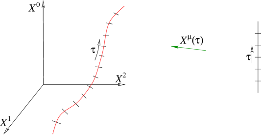
Figure 1: A particle’s world-line. The function $X^{\mu}(\tau)$ embeds the world-line, parametrised by $\tau$, into spacetime, coordinatised by $X^{\mu}$.

The infinitesimal path length swept out is:

$$d\ell=(-ds^{2})^{1/2}=(-dX^{\mu}dX^{\nu}\eta_{\mu\nu})^{1/2}=(-dX^{\mu}dX_{\mu})^{1/2}\ ,$$ (1)

and so the action is

$$S=-m\int d\ell=-m\int d\tau(-{\dot{X}}^{\mu}{\dot{X}}_{\mu})^{1/2}\ ,$$ (2)

where a dot denotes differentiation with respect to $\tau$. Let us vary the action:

$$\delta S=m\int d\tau(-{\dot{X}}^{\mu}{\dot{X}}_{\mu})^{-1/2}{\dot{X}}^{\nu}\delta{\dot{X}}_{\nu}=m\int d\tau u^{\nu}\delta{\dot{X}}_{\nu}=-m\int d\tau{\dot{u}}^{\nu}\delta X_{\nu}\ ,$$ (3)

where the last step used integration by parts, and

$$u^{\nu}\equiv(-{\dot{X}}^{\mu}{\dot{X}}_{\mu})^{-1/2}{\dot{X}}^{\nu}\ .$$ (4)

So for $\delta X$ arbitrary, we get ${\dot{u}}^{\nu}=0$, Newton’s Law of motion.

There is another action from which we can derive the same physics. Consider the action

$$S^{\prime}={1\over 2}\int d\tau\left(\eta^{-1}{\dot{X}}^{\mu}{\dot{X}}_{\mu}-\eta m^{2}\right)\ ,$$ (5)

for some independent function $\eta(\tau)$ defined on the world-line.

N.B.: In preparation for the coming treatment of strings, think of the function $\eta$ as related to the particle’s “world-line metric”, $\gamma_{\tau\tau}$, as $\eta(\tau)=[-\gamma_{\tau\tau}(\tau)]^{1/2}$. The function $\gamma(\tau)$ ensures world-line reparametrisation invariance: $$ds^{2}=\gamma(\tau)_{\tau\tau}d\tau d\tau=\gamma^{\prime}(\tau)_{\tau^{\prime}\tau^{\prime}}d\tau^{\prime}d\tau^{\prime}\ .$$

If we vary $S^{\prime}$ with respect to $\eta$:

$$\delta S^{\prime}={1\over 2}\int d\tau\left[-\eta^{-2}{\dot{X}}^{\mu}{\dot{X}}_{\mu}-m^{2}\right]\delta\eta\ .$$ (6)

So for $\delta\eta$ arbitrary, we get an equation of motion

$$\eta^{2}m^{2}+{\dot{X}}^{\mu}{\dot{X}}_{\mu}=0\ ,$$ (7)

which we can solve with $\eta=m^{-1}(-{\dot{X}}^{\mu}{\dot{X}}_{\mu})^{1/2}$. Upon substituting this into our expression (5) defining $S^{\prime}$, we get:

$$S^{\prime}=-{1\over 2}\int d\tau\left\{m(-{\dot{X}}^{\mu}{\dot{X}}_{\mu})^{1/2}+(-{\dot{X}}^{\mu}{\dot{X}}_{\mu})^{1/2}m^{-1}m\right\}=S\ ,$$ (8)

showing that the two actions are equivalent.

Notice, however, that the action $S^{\prime}$ allows for a treatment of the massless, $m=0$, case, in contrast to $S$. Another attractive feature of $S^{\prime}$ is that it does not use the awkward square root that $S$ does in order to compute the path length. The use of the “auxiliary” parameter $\eta$ allows us to get away from that.

$\bullet\quad{\mbox{\it\it Symmetries}}$

There are two notable symmetries of the action:

• Spacetime Lorentz/Poincaré:

  $$X^{\mu}\to X^{\prime\mu}=\Lambda^{\mu}_{\phantom{\mu}\nu}X^{\nu}+A^{\mu}\ ,$$

  where $\Lambda$ is an $SO(1,3)$ Lorentz matrix and $A^{\mu}$ is an arbitrary constant four–vector. This is a trivial global symmetry of $S^{\prime}$ (and also $S$), following from the fact that we wrote them in covariant form.

• World line Reparametrisations:

  $$\delta X = \zeta(\tau){dX(\tau)\over d\tau}$$

  $$\delta\eta = {d\over d\tau}\left[\zeta(\tau)\eta(\tau)\right]\ ,$$

  for some parameter $\zeta(\tau)$. This is a non–trivial local or “gauge” symmetry. This large extra symmetry on the world-line (and its analogue when we come to study strings) is very useful. We can, for example, use it to pick a nice gauge where we set $\eta=m^{-1}$. This gives a nice simple action, resulting in a simple expression for the conjugate momentum to $X^{\mu}$:

  $$\Pi^{\mu}={\partial{\cal L}\over\partial{\dot{X}}^{\mu}}=m{\dot{X}}^{\mu}$$ (9)

  We will use this much later.

2.2 Classical Bosonic Strings

Turning to strings, we parametrise the “world-sheet” which the string sweeps out with coordinates $(\tau,\sigma)$. The latter is a spatial coordinate, and for now, we take the string to be an open one, with $0\leq\sigma\leq\pi$ running from one end to the other. The string’s evolution in spacetime is described by the functions $X^{\mu}(\tau,\sigma)$, $\mu=0,\cdots,D-1$, giving the shape of the string’s world-sheet in target spacetime (see figure 2).

Figure 2: A string’s world-sheet. The function $X^{\mu}(\tau,\sigma)$ embeds the world-sheet, parametrised by $(\tau,\sigma)$, into spacetime, coordinatized by $X^{\mu}$.

There is an “induced metric” on the world-sheet given by

$$h_{ab}=\partial_{a}X^{\mu}\partial_{b}X^{\nu}\eta_{\mu\nu}\ ,$$ (10)

with which we can perform meaningful measurements on the world-sheet as an object embedded in spacetime. Using this, we can define an action analogous to the one we thought of first for the particle, by asking that we extremize the area of the world-sheet:

$$S=-T\int dA=-T\int d\tau d\sigma\left(-{\rm det}h_{ab}\right)^{1/2}\equiv\int d\tau d\sigma\,\,{{\cal L}}({\dot{X}},X^{\prime};\sigma,\tau)\ .$$ (11)

This is:

$$S = -T\int d\tau d\sigma\left[\left({\partial X^{\mu}\over\partial\sigma}{\partial X^{\mu}\over\partial\tau}\right)^{2}-\left({\partial X^{\mu}\over\partial\sigma}\right)^{2}\left({\partial X^{\mu}\over\partial\tau}\right)^{2}\right]^{1/2}$$ (12)

$$= -T\int d\tau d\sigma\left[(X^{\prime}\cdot{\dot{X}})^{2}-X^{\prime 2}{\dot{X}}^{2}\right]^{1/2}\ ,$$

where $X^{\prime}$ means $\partial X/\partial\sigma$. Varying, we have generally:

$$\delta S = \int d\tau d\sigma\left\{{\partial{\cal L}\over\partial{\dot{X}}^{\mu}}\delta{\dot{X}}^{\mu}+{\partial{\cal L}\over\partial X^{\prime\mu}}\delta X^{\prime\mu}\right\}$$

$$= \int d\tau d\sigma\left\{-{\partial\over\partial\tau}{\partial{\cal L}\over\partial{\dot{X}}^{\mu}}-{\partial\over\partial\sigma}{\partial{\cal L}\over\partial X^{\prime\mu}}\right\}\delta X^{\mu}+\int d\tau\left.\left\{{\partial{\cal L}\over\partial X^{\prime\mu}}\delta X^{\prime\mu}\right\}\right|_{\sigma=0}^{\sigma=\pi}\ .$$

Asking this to be zero, we get:

$${\partial\over\partial\tau}{\partial{\cal L}\over\partial{\dot{X}}^{\mu}}+{\partial\over\partial\sigma}{\partial{\cal L}\over\partial X^{\prime\mu}}=0\quad{\rm and}\quad{\partial{\cal L}\over\partial X^{\prime\mu}}=0\quad{\rm at}\quad\sigma=0,\pi\ ,$$ (14)

which are statements about the conjugate momenta:

$${\partial\over\partial\tau}P^{\mu}_{\tau}+{\partial\over\partial\sigma}P^{\mu}_{\sigma}=0\quad{\rm and}\quad P^{\mu}_{\sigma}=0\quad{\rm at}\quad\sigma=0,\pi\ .$$ (15)

Here, $P^{\mu}_{\sigma}$ is the momentum running along the string (i.e., in the $\sigma$ direction) while $P^{\mu}_{\tau}$ is the momentum running transverse to it. The total spacetime momentum is given by integrating up the infinitesimal (see figure 3):

$$dP^{\mu}=P^{\mu}_{\tau}d\sigma+P^{\mu}_{\sigma}d\tau\ .$$ (16)

Actually, we can choose any slice of the world-sheet in order to compute this momentum. A most convenient one is a slice $d\tau=0$, revealing the string in its original paramaterisation: $P^{\mu}=\int P^{\mu}_{\tau}d\sigma$, but any other slice will do.

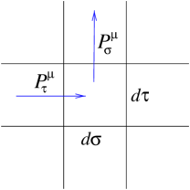
Figure 3: The infinitessimal momenta on the world sheet.

Similarly, one can define the angular momentum:

$$M^{\mu\nu}=\int(P^{\mu}_{\tau}X^{\nu}-P^{\nu}_{\tau}X^{\mu})d\sigma\ .$$ (17)

It is a simple exercise to work out the momenta for our particular Lagrangian:

$$P^{\mu}_{\tau} = T\,{{\dot{X}}^{\mu}X^{\prime 2}-X^{\prime\mu}({\dot{X}}\cdot X^{\prime})\over\sqrt{({\dot{X}}\cdot X^{\prime})^{2}-{\dot{X}}^{2}X^{\prime 2}}}$$

$$P^{\mu}_{\sigma} = T\,{X^{\prime\mu}{\dot{X}}^{2}-{\dot{X}}^{\mu}({\dot{X}}\cdot X^{\prime})\over\sqrt{({\dot{X}}\cdot X^{\prime})^{2}-{\dot{X}}^{2}X^{\prime 2}}}\ .$$ (18)

It is interesting to compute the square of $P_{\sigma}^{\mu}$ using this, and one finds that

$$P^{2}_{\sigma}\equiv P^{\mu}_{\sigma}P_{\mu\sigma}=-2T^{2}{\dot{X}}^{2}\ .$$ (19)

This is our first (perhaps) non–intuitive classical result. We noticed that $P_{\sigma}$ vanishes at the endpoints, in order to prevent momentum from flowing off the ends of the string. The equation we just derived implies that ${\dot{X}}^{2}=0$ at the endpoints, which is to say that they move at the speed of light. This behaviour is a precursor of much of what we will see in the quantum theory later.

Insert 1: $T$ is for Tension As a first non–trivial example (and to learn that $T$, a mass per unit length, really is the string’s tension) let us consider a closed string at rest lying in the $(X^{1},X^{2})$ plane. We can make it by arranging that the $\sigma=0,\pi$ ends meet, that momentum flows across that join. Such a configuration is: $\displaystyle X^{0}$ $\displaystyle=$ $\displaystyle 2R\tau;$ $\displaystyle X^{1}$ $\displaystyle=$ $\displaystyle R\sin 2\sigma$ $\displaystyle X^{2}$ $\displaystyle=$ $\displaystyle R\cos 2\sigma\ .$ It is worth taking the time to use this to show that one gets $$P^{\mu}_{\tau}=T\,(2R,0,0),\quad P^{\mu}_{\sigma}=T\,(0,2R\sin 2\sigma,-2R\cos 2\sigma)\ ,$$ which is interesting, as a sketch shows: The momentum is flowing around the string (which is lying in a circle of radius $R$). The total momentum is $$P^{\mu}=\int_{0}^{\pi}d\sigma\,P_{\tau}^{\mu}\ .$$ The only non–zero component is the mass–energy: $M=2\pi RT={\rm length}{\times}T\ .$

Just like we did in the point particle case, we can introduce an equivalent action which does not have the square root form that the current one has. Once again, we do it by introducing a independent metric, $\gamma_{ab}(\sigma,\tau)$, on the world-sheet, and write:

$$S^{\prime}=-{1\over 4\pi\alpha^{\prime}}\int d\tau d\sigma(-\gamma)^{1/2}\gamma^{ab}\partial_{a}X^{\mu}\partial_{b}X^{\nu}\eta_{\mu\nu}=-{1\over 4\pi\alpha^{\prime}}\int d^{2}\!\sigma\,(-\gamma)^{1/2}\gamma^{ab}h_{ab}\ .$$ (20)

If we vary $\gamma$, we get

$$\delta S^{\prime}=-{1\over 4\pi\alpha^{\prime}}\int d^{2}\!\sigma\,\left\{-{1\over 2}(-\gamma)^{1/2}\delta\gamma\gamma^{ab}h_{ab}+(-\gamma)^{1/2}\delta\gamma^{ab}h_{ab}\right\}\ .$$ (21)

Using the fact that $\delta\gamma=\gamma\gamma^{ab}\delta\gamma_{ab}=-\gamma\gamma_{ab}\delta\gamma^{ab}$, we get

$$\delta S^{\prime}=-{1\over 4\pi\alpha^{\prime}}\int d^{2}\!\sigma\,(-\gamma)^{1/2}\delta\gamma^{ab}\left\{h_{ab}-{1\over 2}\gamma_{ab}\gamma^{cd}h_{cd}\right\}\ .$$ (22)

Therefore we have

$$h_{ab}-{1\over 2}\gamma_{ab}\gamma^{cd}h_{cd}=0\ ,$$ (23)

from which we can derive

$$\gamma^{ab}h_{ab}=2(-h)^{1/2}(-\gamma)^{-1/2}\ ,$$ (24)

and so substituting into $S^{\prime}$, we recover (just as in the point particle case) that it reduces to the Nambu–Goto action, $S$.

Insert 2: A Rotating Open String As a second non–trivial example consider the following open string rotating at a constant angular velocity in the $(X^{1},X^{2})$ plane. Such a configuration is: $\displaystyle X^{0}$ $\displaystyle=$ $\displaystyle\tau;$ $\displaystyle X^{1}$ $\displaystyle=$ $\displaystyle A\left(\sigma-{\pi\over 2}\right)\cos\omega\tau$ $\displaystyle X^{2}$ $\displaystyle=$ $\displaystyle A\left(\sigma-{\pi\over 2}\right)\sin\omega\tau.$ This is what it looks like (the spinning string is shown in frozen snapshots): It is again a worthwhile exercise to compute $P^{\mu}$, and also $M^{\mu\nu}$. With $J\equiv M^{12}$ and $M\equiv P^{0}$, some algebra shows that $${J\over M^{2}}={1\over 2\pi T}=\alpha^{\prime}\ .$$ This parameter, $\alpha^{\prime}$, is the slope of the celebrated “Regge” trajectories: the straight line plots of $J$ vs. $M^{2}$ seen in nuclear physics in the ’60’s. There remains the determination of the intercept of this straight line graph with the $J$–axis. It turns out to be 1 for the bosonic string as we shall see.

$\bullet\quad{\mbox{\it\it Symmetries}}$

Let us again study the symmetries of the action:

• Spacetime Lorentz/Poincaré:

  $$X^{\mu}\to X^{\prime\mu}=\Lambda^{\mu}_{\phantom{\mu}\nu}X^{\nu}+A^{\mu}\ ,$$

  where $\Lambda$ is an $SO(1,3)$ Lorentz matrix and $A^{\mu}$ is an arbitrary constant four–vector. Just as before this is a trivial global symmetry of $S^{\prime}$ (and also $S$), following from the fact that we wrote them in covariant form.

• Worldsheet Reparametrisations:

  $$\delta X^{\mu} = \zeta^{a}\partial_{a}X^{\mu}$$

  $$\delta\gamma^{ab} = \zeta^{c}\partial_{c}\gamma^{ab}-\partial_{c}\zeta^{a}\gamma^{cb}-\partial_{c}\zeta^{b}\gamma^{ac}\ ,$$ (25)

  for two parameters $\zeta^{a}(\tau,\sigma)$. This is a non–trivial local or “gauge” symmetry. This is a large extra symmetry on the world-sheet of which we will make great use.

• Weyl invariance:

  $$\gamma_{ab}\to\gamma^{\prime}_{ab}={\rm e}^{2\omega}\gamma_{ab}\ ,$$ (26)

  specified by a function $\omega(\tau,\sigma)$. This ability to do local rescalings of the metric results from the fact that we did not have to choose an overall scale when we chose $\gamma^{ab}$ to rewrite $S$ in terms of $S^{\prime}$. This can be seen especially if we rewrite the relation (24) as $(-h)^{-1/2}h_{ab}=(-\gamma)^{-1/2}\gamma_{ab}$.

N.B.: We note here for future use that there are just as many parameters needed to specify the local symmetries (three) as there are independent components of the world-sheet metric. This is very, very useful, as we shall see.

$\bullet\quad{\mbox{\it\it String Equations of Motion}}$

We can get equations of motion for the string by varying our action (20) with respect to the $X^{\mu}$:

$$\delta S^{\prime} = {1\over 2\pi\alpha^{\prime}}\int d^{2}\!\sigma\,\partial_{a}\left\{(-\gamma)^{1/2}\gamma^{ab}\partial_{b}X_{\mu}\right\}\delta X^{\mu}$$ (27)

$$\hskip 56.9055pt-{1\over 2\pi\alpha^{\prime}}\int d\tau\left.(-\gamma)^{1/2}\partial_{\sigma}X_{\mu}\delta X^{\mu}\right|_{\sigma=0}^{\sigma=\pi}\ ,$$

which results in the equations of motion:

$$\partial_{a}\left((-\gamma)^{1/2}\gamma^{ab}\partial_{b}X^{\mu}\right)\equiv(-\gamma)^{1/2}\nabla^{2}X^{\mu}=0\ ,$$ (28)

with either:

$$\left.\matrix{X^{\prime\mu}(\tau,0)=0\cr X^{\prime\mu}(\tau,\pi)=0}\right\}\qquad\matrix{\mbox{Open String}\cr\mbox{(Neumann b.c.'s)}}$$ (29)

or:

$$\matrix{X^{\prime\mu}(\tau,0)=X^{\prime\mu}(\tau,\pi)\cr X^{\mu}(\tau,0)=X^{\mu}(\tau,\pi)\cr\gamma_{ab}(\tau,0)=\gamma_{ab}(\tau,\pi)}\Biggr{\}}\qquad\matrix{\mbox{Closed String}\cr\mbox{(periodic b.c.'s)}}$$ (30)

We shall study the equation of motion (28) and the accompanying boundary conditions a lot later. We are going to look at the standard Neumann boundary conditions mostly, and then consider the case of Dirichlet conditions later, when we uncover D–branes,[6, 7, 8, 11, 13, 14, 15] using T–duality.[12] Notice that we have taken the liberty of introducing closed strings by imposing periodicity (see also insert 1 (p.2.2)).

$\bullet\quad{\mbox{\it\it More terms}}$

Thinking of this theory as a two–dimensional model —consisting of $D$ bosonic fields $X^{\mu}(\tau,\sigma)$ with an action given by (20), it is natural to ask whether there are other terms which we might want to add to the theory.

Given that we are treating the two dimensional metric $\gamma_{ab}$ as a dynamical variable, two other terms spring effortlessly to mind, from the analogy with General Relativity. One is the Einstein–Hilbert action (supplemented with a boundary term):

$$\chi={1\over 4\pi\alpha^{\prime}}\int_{\cal M}d^{2}\!\sigma\,(-\gamma)^{1/2}R+{1\over 2\pi\alpha^{\prime}}\int_{\partial{\cal M}}dsK\ ,$$ (31)

where $R$ is the two–dimensional Ricci scalar on the world-sheet ${\cal M}$, $K$ is the extrinsic curvature on the boundary $\partial{\cal M}$ and the other is:

$$\Theta={1\over 4\pi\alpha^{\prime}}\int_{\cal M}d^{2}\!\sigma\,(-\gamma)^{1/2}\ ,$$ (32)

which is the cosmological term. What is their role here? Well, under a Weyl transformation (26), we see that $(-\gamma)^{1/2}\to e^{2\omega}(-\gamma)^{1/2}$ and $R\to e^{-2\omega}(R-2\nabla^{2}\omega)$, and so $\chi$ is invariant, (because $R$ changes by a total derivative which is cancelled by the variation of $K$) but $\Theta$ is not.

So we will include $\chi$, but not $\Theta$ in what follows. Now, the full string action resembles two–dimensional gravity coupled to $D$ bosonic “matter” fields $X^{\mu}$, and the equations of motion are of course:

$$R_{ab}-{1\over 2}\gamma_{ab}R=T_{ab}\ .$$ (33)

The left hand side vanishes identically in two dimensions, and so there is no dynamics associated to (31). The quantity $\chi$ depends only on the topology of the world sheet and so will only matter when comparing world sheets of different topology. This will arise when we compare results from different orders of string perturbation theory and when we consider interactions.

How does this work? Well, let us sketch it here: Let us add our new term to the action, and consider the string action to be (we will denote it $S$ from now on), and dropping the prime:

$$S={1\over 4\pi\alpha^{\prime}}\int_{\cal M}d^{2}\!\sigma\,g^{1/2}g^{ab}\partial_{a}X^{\mu}\partial_{b}X_{\mu}+\lambda\left\{{1\over 4\pi\alpha^{\prime}}\int_{\cal M}d^{2}\!\sigma\,(g)^{1/2}R+{1\over 2\pi\alpha^{\prime}}\int_{\partial{\cal M}}dsK\right\}\ ,$$ (34)

where $\lambda$ is —for now— and arbitrary parameter which we have not fixed to any particular value.

N.B.: It will turn out that $\lambda$ is not a free parameter. In the full string theory, it has dynamical meaning, and will be equivalent to the expectation value of one of the massless fields —the “dilaton”— described by the string.

Note that we have anticipated something that we will do later, which is to work with Euclidean signature to make sense of the topological statements to follow: $\gamma_{ab}$ with signature $(-+)$ has been replaced by $g_{ab}$ with signature $(++)$.

So what will $\lambda$ do? Recall that it couples to Euler number, so in the full path integral defining the string theory:

$${\cal Z}=\int{\cal D}X{\cal D}g\,\,e^{-S}\ ,$$ (35)

resulting amplitudes will be weighted by a factor $e^{-\lambda\chi}$, where $\chi=2-2h-b-c$. Here, $h,b,c$ are the numbers of handles, boundaries and crosscaps, respectively, on the world sheet. Consider figure 4. An emission and reabsorption of an open string results in a change $\delta\chi=-1$, while for a closed string it is $\delta\chi=-2$. Therefore, relative to the tree level open string diagram (disc topology), the amplitudes are weighted by $e^{\lambda}$ and $e^{2\lambda}$, respectively. The quantity $g_{s}\equiv e^{\lambda}$ therefore will be called the closed string coupling. Note that it is the square of the open string coupling.

Figure 4: Worldsheet topology change due to emission and reabsorption of open and closed strings

$\bullet\quad{\mbox{\it\it The Stress Tensor}}$

Let us also note that we can define a two–dimensional energy–momentum tensor:

$$T^{ab}(\tau,\sigma)\equiv-{4\pi\over\sqrt{-\gamma}}{\delta S\over\delta\gamma_{ab}}=-{1\over\alpha^{\prime}}\left\{\partial^{a}X_{\mu}\partial^{b}X^{\mu}-{1\over 2}\gamma^{ab}\gamma_{cd}\partial^{c}X_{\mu}\partial^{d}X^{\mu}\right\}\ .$$ (36)

Notice that

$$T^{a}_{a}\equiv\gamma_{ab}T^{ab}=0\ .$$ (37)

This is a consequence of Weyl symmetry. Reparametrisation invariance, $\delta_{\gamma}S^{\prime}=0$, translates here into (see discussion after eqn.(33))

$$T^{ab}=0\ .$$ (38)

These are the classical properties of the theory we have uncovered so far. Later on, we shall attempt to ensure that they are true in the quantum theory also, with interesting results.

$\bullet\quad{\mbox{\it\it Gauge Fixing}}$

Now recall that we have three local or “gauge” symmetries of the action:

$$\mbox{2d reparametrisations}:\,\,\sigma,\tau \to {\tilde{\sigma}}(\sigma,\tau),{\tilde{\tau}}(\sigma,\tau)$$

$$\mbox{Weyl}:\,\,\gamma_{ab} \to \exp({2\omega(\sigma,\tau)})\gamma_{ab}\ .$$ (39)

The two dimensional metric $\gamma_{ab}$ is also specified by three independent functions, as it is a symmetric $2\times 2$ matrix. We may therefore use the gauge symmetries (see (25), (26)) to choose $\gamma_{ab}$ to be a particular form:

$$\gamma_{ab}=\eta_{ab}=\pmatrix{-1&0\cr\phantom{-}0&1}\ .$$ (40)

In this “conformal” gauge, our $X^{\mu}$ equations of motion (28) become:

$$\left({\partial^{2}\over\partial\sigma^{2}}-{\partial^{2}\over\partial\tau^{2}}\right)X^{\mu}(\tau,\sigma)=0\ ,$$ (41)

the two dimensional wave equation. As this is $\partial_{\sigma^{+}}\partial_{\sigma^{-}}X^{\mu}=0$, we see that the full solution to the equation of motion can be written in the form:

$$X^{\mu}(\sigma,\tau)=X_{L}^{\mu}(\sigma^{+})+X^{\mu}_{R}(\sigma^{-})\ ,$$ (42)

where $\sigma^{\pm}\equiv\tau\pm\sigma$.

N.B.: Write $\sigma^{\pm}=\tau\pm\sigma$. This gives metric $ds^{2}=-d\tau^{2}+d\sigma^{2}\to-d\sigma^{+}d\sigma^{-}.$ So we have $\eta_{-+}=\eta_{+-}=-1/2$, $\eta^{-+}=\eta^{+-}=-2$ and $\eta_{++}=\eta_{--}=\eta^{++}=\eta^{--}=0$. Also, $\partial_{\tau}=\partial_{+}+\partial_{-}$ and $\partial_{\sigma}=\partial_{+}-\partial_{-}$.

Our constraints on the stress tensor become:

$$T_{\tau\sigma} = T_{\sigma\tau}\equiv{1\over\alpha^{\prime}}{\dot{X}}^{\mu}X^{\prime}_{\mu}=0$$

$$T_{\sigma\sigma} = T_{\tau\tau}={1\over 2\alpha^{\prime}}\left({\dot{X}}^{\mu}{\dot{X}}_{\mu}+X^{\prime}\!{}^{\mu}X^{\prime}_{\mu}\right)=0\ ,$$ (43)

or

$$T_{++} = {1\over 2}(T_{\tau\tau}+T_{\tau\sigma})={1\over\alpha^{\prime}}\partial_{+}X^{\mu}\partial_{+}X_{\mu}\equiv{1\over\alpha^{\prime}}{\dot{X}}^{2}_{L}=0$$

$$T_{--} = {1\over 2}(T_{\tau\tau}-T_{\tau\sigma})={1\over\alpha^{\prime}}\partial_{-}X^{\mu}\partial_{-}X_{\mu}\equiv{1\over\alpha^{\prime}}{\dot{X}}^{2}_{R}=0\ ,$$ (44)

and $T_{-+}$ and $T_{+-}$ are identically zero.

$\bullet\quad{\mbox{\it\it The Mode Decomposition}}$

Our equations of motion (42), with our boundary conditions (29) and (30) have the simple solutions:

$$X^{\mu}(\tau,\sigma)=x^{\mu}+2\alpha^{\prime}p^{\mu}\tau+i(2\alpha^{\prime})^{1/2}\sum_{n\neq 0}{1\over n}\alpha_{n}^{\mu}e^{-in\tau}\cos n\sigma\ ,$$ (45)

for the open string and

$$X^{\mu}(\tau,\sigma) = X^{\mu}_{R}(\sigma^{-})+X_{L}^{\mu}(\sigma^{+})$$

$$X^{\mu}_{R}(\sigma^{-}) = {1\over 2}x^{\mu}+\alpha^{\prime}p^{\mu}\sigma^{-}+i\left({\alpha^{\prime}\over 2}\right)^{1/2}\sum_{n\neq 0}{1\over n}\alpha_{n}^{\mu}e^{-2in\sigma^{-}}$$

$$X^{\mu}_{L}(\sigma^{+}) = {1\over 2}x^{\mu}+\alpha^{\prime}p^{\mu}\sigma^{+}+i\left({\alpha^{\prime}\over 2}\right)^{1/2}\sum_{n\neq 0}{1\over n}{\tilde{\alpha}}_{n}^{\mu}e^{-2in\sigma^{+}}\ ,$$ (46)

for the closed string, where, to ensure a real solution we impose $\alpha_{-n}^{\mu}=(\alpha_{n}^{\mu})^{*}$ and ${\tilde{\alpha}}_{-n}^{\mu}=({\tilde{\alpha}}_{n}^{\mu})^{*}$. Note that $x^{\mu}$ and $p^{\mu}$ are the centre of mass position and momentum, respectively. In each case, we can identify $p^{\mu}$ with the zero mode of the expansion:

$$\mbox{open string:}\qquad\,\,\alpha_{0}^{\mu} = (2\alpha^{\prime})^{1/2}p^{\mu};$$

$$\mbox{closed string:}\qquad\,\,\alpha_{0}^{\mu} = \left({\alpha^{\prime}\over 2}\right)^{1/2}p^{\mu}\ .$$ (47)

N.B.: Notice that the mode expansion for the closed string (46) is simply that of a pair of independent left and right moving travelling waves going around the string in opposite directions. The open string expansion (45) on the other hand, has a standing wave for its solution, representing the left and right moving sector reflected into one another by the Neumann boundary condition (29).

$\bullet\quad{\mbox{\it\it A Residual Symmetry}}$

Actually, we have not gauged away all of the local symmetry by choosing the gauge (40). We can do a left–right decoupled change of variables:

$$\sigma^{+}\to f(\sigma^{+})=\sigma^{\prime+};\,\,\sigma^{-}\to g(\sigma^{-})=\sigma^{\prime-}\ .$$ (48)

Then, as

$$\gamma^{\prime}_{ab}={\partial\sigma^{c}\over\partial\sigma^{\prime a}}{\partial\sigma^{d}\over\partial\sigma^{\prime b}}\gamma_{cd}\ ,$$ (49)

we have

$$\gamma^{\prime}_{+-}=\left({\partial f(\sigma^{+})\over\partial\sigma^{+}}{\partial g(\sigma^{-})\over\partial\sigma^{-}}\right)^{-1}\gamma_{+-}\ .$$ (50)

However, we can undo this with a Weyl transformation of the form

$$\gamma^{\prime}_{+-}=\exp(2\omega_{L}(\sigma^{+})+2\omega_{R}(\sigma^{-}))\gamma_{+-}\ ,$$ (51)

if $\exp(-2\omega_{L}(\sigma^{+}))=\partial_{+}f(\sigma^{+})$ and $\exp(-2\omega_{R}(\sigma^{-}))=\partial_{-}g(\sigma^{-})$. So we still have a residual “conformal” symmetry. As $f$ and $g$ are independent arbitrary functions on the left and right, we have an infinite number of conserved quantities on the left and right. This is because the conservation equation $\nabla_{a}T^{ab}=0$, together with the result $T_{+-}=T_{-+}=0$, turns into:

$$\partial_{-}T_{++}=0\quad\mbox{and}\quad\partial_{+}T_{--}=0\ ,$$ (52)

but since $\partial_{-}f=0=\partial_{+}g$, we have

$$\partial_{-}(f(\sigma^{+})T_{++})=0\quad\mbox{and}\quad\partial_{+}(g(\sigma^{-})T_{--})=0\ ,$$ (53)

resulting in an infinite number of conserved quantities. The fact that we have this infinite dimensional conformal symmetry is the basis of some of the most powerful tools in the subject, for computing in perturbative string theory.

$\bullet\quad{\mbox{\it\it Hamiltonian Dynamics}}$

Our Lagrangian density is

$${\cal L}=-{1\over 4\pi\alpha^{\prime}}\left(\partial_{\sigma}X^{\mu}\partial_{\sigma}X_{\mu}-\partial_{\tau}X^{\mu}\partial_{\tau}X_{\mu}\right)\ ,$$ (54)

from which we can derive that the conjugate momentum to $X^{\mu}$ is

$$\Pi^{\mu}={\delta{\cal L}\over\delta(\partial_{\tau}X^{\mu})}={1\over 2\pi\alpha^{\prime}}{\dot{X}}^{\mu}\ .$$ (55)

So we have the equal time Poisson brackets:

$$\left[X^{\mu}(\sigma),\Pi^{\nu}(\sigma^{\prime})\right]_{\rm P.B.}=\eta^{\mu\nu}\delta(\sigma-\sigma^{\prime})\ ,$$ (56)

$$\left[\Pi^{\mu}(\sigma),\Pi^{\nu}(\sigma^{\prime})\right]_{\rm P.B.}=0\ ,$$ (57)

with the following results on the oscillator modes:

$$\left[\alpha_{m}^{\mu},\alpha_{n}^{\nu}\right]_{\rm P.B.} = \left[{\tilde{\alpha}}_{m}^{\mu},{\tilde{\alpha}}_{n}^{\nu}\right]_{\rm P.B.}=im\delta_{m+n}\eta^{\mu\nu}$$

$$\left[p^{\mu},x^{\nu}\right]_{\rm P.B.} = \eta^{\mu\nu};\quad\left[\alpha_{m}^{\mu},{\tilde{\alpha}}_{n}^{\nu}\right]_{\rm P.B.}=0\ .$$ (58)

We can form the Hamiltonian density

$${\cal H}={\dot{X}}^{\mu}\Pi_{\mu}-{\cal L}={1\over 4\pi\alpha^{\prime}}\left(\partial_{\sigma}X^{\mu}\partial_{\sigma}X_{\mu}+\partial_{\tau}X^{\mu}\partial_{\tau}X_{\mu}\right)\ ,$$ (59)

from which we can construct the Hamiltonian $H$ by integrating along the length of the string. This results in:

$$H = \int_{0}^{\pi}d\sigma\,{\cal H}(\sigma)={1\over 2}\sum_{-\infty}^{\infty}\alpha_{-n}\cdot\alpha_{n}\qquad\mbox{(open)}$$

$$H = \int_{0}^{2\pi}d\sigma\,{\cal H}(\sigma)={1\over 2}\sum_{-\infty}^{\infty}\left(\alpha_{-n}\cdot\alpha_{n}+{\tilde{\alpha}}_{-n}\cdot{\tilde{\alpha}}_{n}\right)\qquad\mbox{(closed)}\ .$$ (60)

(We have used the notation $\alpha_{n}\cdot\alpha_{n}\equiv\alpha^{\mu}_{n}\alpha_{n\mu}$) The constraints $T_{++}=0=T_{--}$ on our energy–momentum tensor can be expressed usefully in this language. We impose them mode by mode in a Fourier expansion, defining:

$$L_{m}={T\over 2}\int_{0}^{\pi}e^{-2im\sigma}T_{--}d\sigma={1\over 2}\sum_{-\infty}^{\infty}\alpha_{m-n}\cdot\alpha_{n}\ ,$$ (61)

and similarly for ${\bar{L}}_{m}$, using $T_{++}$. Using the Poisson brackets (58), these can be shown to satisfy the “Virasoro” algebra:

$$\left[L_{m},L_{n}\right]_{\rm P.B.} = i(m-n)L_{m-n};\quad\left[{\bar{L}}_{m},{\bar{L}}_{n}\right]_{\rm P.B.}=i(m-n){\bar{L}}_{m-n};$$

$$\left[{\bar{L}}_{m},L_{n}\right]_{\rm P.B.} = 0\ .$$ (62)

Notice that there is a nice relation between the zero modes of our expansion and the Hamiltonian:

$$H=L_{0}\qquad\mbox{(open)};\quad H=L_{0}+{\bar{L}}_{0}\qquad\mbox{(closed)}\ .$$ (63)

So to impose our constraints, we can do it mode by mode and ask that $L_{m}=0$ and ${\bar{L}}_{m}=0$, for all $m$. Looking at the zeroth constraint results in something interesting. Note that

$$L_{0} = {1\over 2}\alpha_{0}^{2}+2\times{1\over 2}\sum_{n=1}^{\infty}\alpha_{-n}\cdot\alpha_{n}+{D\over 2}\sum_{n=1}^{\infty}n$$ (64)

$$= \alpha^{\prime}p^{\mu}p_{\mu}+\sum_{n=1}^{\infty}\alpha_{-n}\cdot\alpha_{n}+{\rm const}$$

$$= -\alpha^{\prime}M^{2}+\sum_{n=1}^{\infty}\alpha_{-n}\cdot\alpha_{n}+{\rm const}\ ,$$

where the constant is suspiciously infinite. We will ignore it for now, and discuss it in the next section, where we study the quantum theory. Requiring $L_{0}$ to be zero —diffeomorphism invariance— results in a (spacetime) mass relation:

$$M^{2}={1\over\alpha^{\prime}}\sum_{n=1}^{\infty}\alpha_{-n}\cdot\alpha_{n}\qquad\mbox{(open)}\ ,$$ (65)

where we have used the zero mode relation (47) for the open string. A similar exercise produces the mass relation for the closed string:

$$M^{2}={2\over\alpha^{\prime}}\sum_{n=1}^{\infty}\left(\alpha_{-n}\cdot\alpha_{n}+{\tilde{\alpha}}_{-n}\cdot{\tilde{\alpha}}_{n}\right)\qquad\mbox{(closed)}\ .$$ (66)

These formulae (65) and (66) give us the result for the mass of a state in terms of how many oscillators are excited on the string. The masses are set by the string tension $T=(2\pi\alpha^{\prime})^{-1}$, as they should be. Let us not dwell for too long on these formulae however, as they are significantly modified when we quantise the theory, since we have to understand the infinite constant which we ignored.

2.3 Quantised Bosonic Strings

For our purposes, the simplest route to quantisation will be to promote everything we met previously to operator statements, replacing Poisson Brackets by commutators in the usual fashion: $[\phantom{X},\phantom{X}]_{\rm P.B.}\to-i[\phantom{X},\phantom{X}]$. This gives:

$$\left[X^{\mu}(\tau,\sigma),\Pi^{\nu}(\tau,\sigma^{\prime})\right] = i\eta^{\mu\nu}\delta(\sigma-\sigma^{\prime})\ ;\quad\left[\Pi^{\mu}(\tau,\sigma),\Pi^{\nu}(\tau,\sigma^{\prime})\right]=0$$

$$\left[\alpha_{m}^{\mu},\alpha_{n}^{\nu}\right] = \left[{\tilde{\alpha}}_{m}^{\mu},{\tilde{\alpha}}_{n}^{\nu}\right]\,=\,m\delta_{m+n}\eta^{\mu\nu}$$

$$\left[x^{\nu},p^{\mu}\right] = i\eta^{\mu\nu};\quad\left[\alpha_{m}^{\mu},{\tilde{\alpha}}_{n}^{\nu}\right]\,=\,0\ .$$ (67)

N.B.: One of the first things that we ought to notice here is that $\sqrt{m}\alpha_{\pm m}^{\mu}$ are like creation and annihilation operators for the harmonic oscillator. There are actually $D$ independent families of them —one for each spacetime dimension— labelled by $\mu$.

In the usual fashion, we will define our Fock space such that $|0;k\!>$ is an eigenstate of $p^{\mu}$ with centre of mass momentum $k^{\mu}$. This state is annihilated by $\alpha^{\nu}_{m}$.

What about our operators, the $L_{m}$? Well, with the usual “normal ordering” prescription that all annihilators are to the right, the $L_{m}$ are all fine when promoted to operators, except the Hamiltonian, $L_{0}$. It needs more careful definition, since $\alpha^{\mu}_{n}$ and $\alpha^{\mu}_{-n}$ do not commute. Indeed, as an operator, we have that

$$L_{0}={1\over 2}\alpha_{0}^{2}+\sum_{n=1}^{\infty}\alpha_{-n}\cdot\alpha_{n}+\mbox{constant}\ ,$$ (68)

where the apparently infinite constant is composed as copy of the infinite sum $(1/2)\sum_{n=1}^{\infty}n$ for each of the $D$ families of oscillators. As is of course to be anticipated, this infinite constant can be regulated to give a finite answer, corresponding to the total zero point energy of all of the harmonic oscillators in the system.

$\bullet\quad{\mbox{\it The Constraints and Physical States}}$

For now, let us not worry about the value of the constant, and simply impose our constraints on a state $|\phi\!>$ as:

$$(L_{0}-a)|\phi\!>=0;\qquad L_{m}|\phi\!>=0\quad\mbox{for }m>0\ ,$$ (69)

where our infinite constant is set by $a$, which is to be computed. There is a reason why we have not also imposed this constraint for the $L_{-m}$’s. This is because the Virasoro algebra (62) in the quantum case is:

$$\left[L_{m},L_{n}\right] = (m-n)L_{m-n}+{D\over 12}(m^{3}-m)\delta_{m+n};\quad\left[{\bar{L}}_{m},L_{n}\right]=0;$$

$$\left[{\bar{L}}_{m},{\bar{L}}_{n}\right] = (m-n){\bar{L}}_{m-n}+{D\over 12}(m^{3}-m)\delta_{m+n}\ ,$$ (70)

There is a central term in the algebra, which produces a non–zero constant when $m=n$. Therefore, imposing both $L_{m}$ and $L_{-m}$ would produce an inconsistency.

Note now that the first of our constraints (69) produces a modification to the mass formulae:

$$M^{2} = {1\over\alpha^{\prime}}\left(\sum_{n=1}^{\infty}\alpha_{-n}\cdot\alpha_{n}-a\right)\qquad\mbox{(open)}$$

$$M^{2} = {2\over\alpha^{\prime}}\left(\sum_{n=1}^{\infty}\left(\alpha_{-n}\cdot\alpha_{n}+{\tilde{\alpha}}_{-n}\cdot{\tilde{\alpha}}_{n}\right)-2a\right)\qquad\mbox{(closed)}\ .$$ (71)

Notice that we can denote the (weighted) number of oscillators excited as $N=\sum\alpha_{-n}\cdot\alpha_{n}$ $(=\sum nN_{n})$ on the left and ${\bar{N}}=\sum{\tilde{\alpha}}_{-n}\cdot{\tilde{\alpha}}_{n}$ $(=\sum n{\bar{N}}_{n})$ on the right. $N_{n}$ and ${\bar{N}}_{n}$ are the true count, on the left and right, of the number of copies of the oscillator labelled by $n$ is present.

There is an extra condition in the closed string case. While $L_{0}+{\bar{L}}_{0}$ generates time translations on the world sheet (being the Hamiltonian), the combination $L_{0}-{\bar{L}}_{0}$ generates translations in $\sigma$. As there is no physical significance to where on the string we are, the physics should be invariant under translations in $\sigma$, and we should impose this as an operator condition on our physical states:

$$(L_{0}-{\bar{L}}_{0})|\phi>=0\ ,$$ (72)

which results in the “level–matching” condition $N={\bar{N}}$, equating the number of oscillators excited on the left and the right.

In summary then, we have two copies of the open string on the left and the right, in order to construct the closed string. The only extra subtlety is that we should use the correct zero mode relation (47) and match the number of oscillators on each side according to the level matching condition (72).

$\bullet\quad{\mbox{\it The Intercept and Critical Dimensions}}$

Let us consider the spectrum of states level by level, and uncover some of the features, focusing on the open string sector. Our first and simplest state is at level 0, i.e., no oscillators excited at all. There is just some centre of mass momentum that it can have, which we shall denote as $k$. Let us write this state as $|0;k\!>$. The first of our constraints (69) leads to an expression for the mass:

$$(L_{0}-a)|0;k\!>=0\qquad\Rightarrow\alpha^{\prime}k^{2}=a,\qquad\mbox{so }M^{2}=-{a\over\alpha^{\prime}}\ .$$ (73)

This state is a tachyonic state, having negative mass–squared.

The next simplest state is that with momentum $k$, and one oscillator excited. We are also free to specify a polarisation vector $\zeta^{\mu}$. We denote this state as $|\zeta,k>\equiv(\zeta\cdot\alpha_{-1})|0;k\!>$; it starts out the discussion with $D$ independent states. The first thing to observe is the norm of this state:

$$<\!\zeta;k||\zeta;k^{\prime}\!> = <\!0;k|\zeta^{*}\cdot\alpha_{1}\zeta\cdot\alpha_{-1}|0;k^{\prime}\!>$$ (74)

$$= \zeta^{*\mu}\zeta^{\nu}<\!0;k|\alpha^{\mu}_{1}\cdot\alpha^{\nu}_{-1}|0;k^{\prime}\!>$$

$$= \zeta\cdot\zeta<\!0;k|0;k^{\prime}\!>=\zeta\cdot\zeta(2\pi)^{D}\delta^{D}(k-k^{\prime})\ ,$$

where we have used the commutator (67) for the oscillators. From this we see that the time-like component of $\zeta$ will produce a state with negative norm. Such states cannot be made sense of in a unitary theory, and are often called “ghosts”.

Let us study the first constraint:

$$(L_{0}-a)|\zeta;k\!>=0\qquad\Rightarrow\quad\alpha^{\prime}k^{2}+1=a,\qquad M^{2}={1-a\over\alpha^{\prime}}\ .$$ (75)

The next constraint gives:

$$(L_{1})|\zeta;k\!>=\sqrt{\alpha^{\prime}\over 2}k\cdot\alpha_{1}\zeta\cdot\alpha_{-1}|0;k>=0\qquad\Rightarrow,\qquad k\cdot\zeta=0\ .$$ (76)

Actually, at level 1, we can also make a special state of interest: $|\psi\!>\equiv L_{-1}|0;k\!>$. This state has the special property that it is orthogonal to any physical state, since $<\!\phi|\psi\!>=<\!\psi|\phi\!>^{*}=<\!0;k|L_{1}|\phi\!>=0$. It also has $L_{1}|\psi\!>=2L_{0}|0;k\!>=\alpha^{\prime}k^{2}|0;k>.$ This state is called a “spurious” state.

So we note that there are three interesting cases for the level 1 physical state we have been considering:

1. $a<1\Rightarrow M^{2}>0:$

   • momentum $k$ is timelike.

   • We can choose a frame where it is $(k,0,0,\ldots)$

   • Spurious state is not physical, since $k^{2}\neq 0$.

   • $k\cdot\zeta=0$ removes the timelike polarisation. $D-1$ states left

2. $a>1\Rightarrow M^{2}<0:$

   • momentum $k$ is spacelike.

   • We can choose a frame where it is $(0,k_{1},k_{2},\ldots)$

   • Spurious state is not physical, since $k^{2}\neq 0$

   • $k\cdot\zeta=0$ removes a spacelike polarisation. $D-1$ states left, one which is including ghosts and tachyons.

3. $a=1\Rightarrow M^{2}=0:$

   • momentum $k$ is null.

   • We can choose a frame where it is $(k,k,0,\ldots)$

   • Spurious state is physical and null, since $k^{2}=0$

   • $k\cdot\zeta=0$ and $k^{2}=0$ removes two polarisations; $D-2$ states left

So if we choose case (3), we end up with the special situation that we have a massless vector in the $D$ dimensional target spacetime. It even has an associated gauge invariance: since the spurious state is physical and null, and therefore we can add it to our physical state with no physical consequences, defining an equivalence relation:

$$|\phi>\sim|\phi>+\lambda|\psi>\qquad\Rightarrow\qquad\zeta^{\mu}\sim\zeta^{\mu}+\lambda k^{\mu}\ .$$ (77)

Case (1), while interesting, corresponds to a massive vector, where the extra state plays the role of a longitudinal component. Case (2) seems bad. We shall choose case (3), where $a=1$.

It is interesting to proceed to level two to construct physical and spurious states, although we shall not do it here. The physical states are massive string states. If we insert our level one choice $a=1$ and see what the condition is for the maximal space spurious states to be both physical and null, we find that there is a condition on the spacetime dimension: $D=26$.

In summary, we see that $a=1$, $D=26$ for the open bosonic string gives a family of extra null states, giving something analogous to a point of “enhanced gauge symmetry” in the space of possible string theories. This is called a “critical” string theory, for many reasons. We have the 24 states of a massless vector we shall loosely called the photon, $A_{\mu}$, since it has a $U(1)$ gauge invariance (77). There is a tachyon of $M^{2}=-1/\alpha^{\prime}$ in the spectrum, which will not trouble us unduly. We will actually remove it in going to the superstring case. Tachyons will reappear from time to time, representing situations where we have an unstable configuration (as happens in field theory frequently). Generally, it seems that we should think of tachyons in the spectrum as pointing us towards an instability, and in many cases, the source of the instability is manifest. Indeed, this will be put to good use in constructing stable non–BPS D–brane solitons in the lectures of John Schwarz in this TASI school[18], following a recently developed technique of Sen. [16] In these lectures, we will try to map out the supersymmetric landscape, but ocassionally this line of reasoning will appear.

Our analysis here extends to the closed string, since we can take two copies of our result, use the appropriate zero mode relation (47), and level matching. At level zero we get the closed string tachyon which has $M^{2}=-4/\alpha^{\prime}$. At level zero we get a tachyon with mass given by $M^{2}=-4/\alpha^{\prime}$, and at level 1 we get 24² massless states from $\alpha^{\mu}_{-1}{\tilde{\alpha}}^{\nu}_{-1}|0;k\!>$. The traceless symmetric part is the graviton, $G_{\mu\nu}$ and the antisymmetric part, $B_{\mu\nu}$, is sometimes called the Kalb–Ramond field, and the trace is is the dilaton, $\Phi$.

$\bullet\quad{\mbox{\it Had We Been More Careful}}$

A more careful treatment of our gauge fixing procedure (40) would had seen us introduce Faddev–Popov ghosts $(b,c)$ (i.e., friendly ghosts) to ensure that we stay on our chosen gauge slice in the full theory. Our resulting two dimensional conformal field theory would have had an extra sector coming from the $(b,c)$ ghosts.

The central term in the Virasoro algebra (70) represents an anomaly in the transformation properties of the stress tensor, spoiling its properties as a tensor under general coordinate transformations. Generally:

$$\left({\partial\sigma^{\prime+}\over\partial\sigma^{+}}\right)^{2}T^{\prime}_{++}(\sigma^{\prime+})=T_{++}(\sigma^{+})-{{\rm c}\over 12}\left\{{2\partial_{\sigma}^{3}\sigma^{\prime}\partial_{\sigma}\sigma^{\prime}-3\partial_{\sigma}^{2}\sigma^{\prime}\partial^{2}_{\sigma}\sigma^{\prime}\over 2\partial_{\sigma}\sigma^{\prime}\partial_{\sigma}\sigma^{\prime}}\right\}\ ,$$ (78)

where $\rm c$ is a number which depends upon the content of the theory. In our case, we have $D$ bosons, which each contribute $1$ to c, for a total anomaly of $D$.

The ghosts do two crucial things: They contribute to the anomaly the amount $-26$, and therefore we can retain all our favourite symmetries for the dimension $D=26$. They also cancel the contributions to the vacuum energy coming from the oscillators in the $\mu=0,1$ sector, leaving $D-2$ transverse oscillators’ contribution.

The regulated value of $-a$ is the vacuum or “zero point energy” (z.p.e.) of the transverse modes of the theory. This zero point energy is simply the Casimir energy arising from the fact that the two dimensional field theory is in a box. The box is the infinite strip, for the case of an open string, or the infinite cylinder, for the case of the closed string (see figure 5).

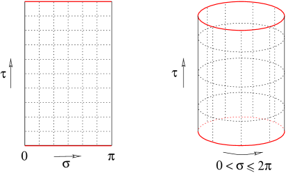
Figure 5: String worldsheets as boxes upon which live two dimensional conformal field theory.

A periodic (integer moded) boson such as the types we have here, $X^{\mu}$, each contribute $-1/24$ to the vacuum energy (see insert 3 (p.2.3)on a quick way to compute this). So we see that in 26 dimensions, with only 24 contributions to count (see previous paragraph), we get that $-a=24\times(-1/24)=-1$. (Notice that from (64), this implies that $\sum_{n=1}^{\infty}n=-1/12$, which is in fact true in $\zeta$–function regularisation.)

Later, we shall have world sheet fermions $\psi^{\mu}$ as well, in the supersymmetric theory. They each contribute $1/2$ to the anomaly. World sheet superghosts will cancel the contributions from $\psi^{0},\psi^{1}$. Each anti–periodic fermion will give a z.p.e. contribution of $-1/48$.

Generally, taking into account the possibility of both periodicities for either bosons or fermions:

z.p.e. $$= {1\over 2}\omega\qquad\mbox{for boson};\qquad-{1\over 2}\omega\qquad\mbox{for fermion}$$

$$\omega = {1\over 24}-{1\over 8}(2\theta-1)^{2}\qquad\left\{\matrix{\theta&=&0&\quad\mbox{(integer modes)}\cr\theta&=&{1\over 2}&\quad\mbox{(half--integer modes)}}\right.\,$$ (79)

This is a formula which we shall use many times in what is to come.

Insert 3: Cylinders, Strips and the Complex Plane As promised earlier, we will go from Lorentzian to Euclidean signature (making the action real) by sending $\tau\to i\tau$. Another thing we will often do is work on the complex plane, instead of the original world sheets we started with. We go from one to the other using the exponential map, defining a complex coordinate on the plane $z=e^{\tau-i\sigma}=e^{w}$. The closed string’s cylinder and the open string’s strip (see figure 5) map to the complex plane and the (upper) half complex plane, respectively: Note that the Fourier expansions we have been working with to define the modes become Laurent expansions on the complex plane, e.g.: $$T_{zz}(z)=\sum_{m=-\infty}^{\infty}{L_{m}\over z^{m+2}}\ .$$ One of the most straightforward exercises is to compute the zero point energy of the cylinder or strip (for a field of central charge $c$) by starting with the fact that the plane has no Casimir energy. One simply plugs the exponential change of coordinates $z=e^{w}$ into the anomalous transformation for the energy momentum tensor and compute the contribution to $T_{ww}$ starting with $T_{zz}$: $$T_{ww}=-z^{2}T_{zz}-{c\over 24}\ ,$$ which results in the Fourier expansion on the cylinder, in terms of the modes: $$T_{ww}(w)=-\sum_{m=-\infty}^{\infty}\left(L_{m}-{c\over 24}\delta_{m,0}\right)e^{i\sigma-\tau}\ .$$

$\bullet\quad{\mbox{\it States and Operators}}$

As we learned in insert 3, (p.2.3) we can work on the complex plane with coordinate $z$. In these coordinates, our mode expansions (45) and (46) become:

$$X^{\mu}(z,\bar{z})=x^{\mu}-i\left({\alpha^{\prime}\over 2}\right)^{1/2}\alpha^{\mu}_{0}\ln z\bar{z}+i\left({\alpha^{\prime}\over 2}\right)^{1/2}\sum_{n\neq 0}{1\over n}\alpha_{n}^{\mu}\left(z^{-n}+\bar{z}^{-n}\right)\ ,$$ (80)

for the open string, and for the closed:

$$X^{\mu}(z,\bar{z}) = X^{\mu}_{L}(z)+X_{R}^{\mu}(\bar{z})$$

$$X^{\mu}_{L}(z) = {1\over 2}x^{\mu}-i\left({\alpha^{\prime}\over 2}\right)^{1/2}\alpha^{\mu}_{0}\ln z+i\left({\alpha^{\prime}\over 2}\right)^{1/2}\sum_{n\neq 0}{1\over n}\alpha_{n}^{\mu}z^{-n}$$

$$X^{\mu}_{R}(\bar{z}) = {1\over 2}x^{\mu}-i\left({\alpha^{\prime}\over 2}\right)^{1/2}{\tilde{\alpha}}^{\mu}_{0}\ln\bar{z}+i\left({\alpha^{\prime}\over 2}\right)^{1/2}\sum_{n\neq 0}{1\over n}{\tilde{\alpha}}_{n}^{\mu}\bar{z}^{-n}\ ,$$ (81)

where we have used the zero mode relations (47). In fact, notice that:

$$\partial_{z}X^{\mu}(z) = -i\left({\alpha^{\prime}\over 2}\right)^{1/2}\sum_{n}{\alpha}_{n}^{\mu}z^{-n-1}$$

$$\partial_{\bar{z}}X^{\mu}(\bar{z}) = -i\left({\alpha^{\prime}\over 2}\right)^{1/2}\sum_{n}{\tilde{\alpha}}_{n}^{\mu}\bar{z}^{-n-1}\ ,$$ (82)

and that we can invert these to get (for the closed string)

$${\alpha}_{-n}^{\mu}=\left({2\over\alpha^{\prime}}\right)^{1/2}\oint{dz\over 2\pi}z^{-n}\partial_{z}X^{\mu}(z)\qquad{\tilde{\alpha}}_{-n}^{\mu}=\left({2\over\alpha^{\prime}}\right)^{1/2}\oint{dz\over 2\pi}\bar{z}^{-n}\partial_{\bar{z}}X^{\mu}(z)\ ,$$ (83)

which are non–zero for $n\geq 0$. This is suggestive: Equations (82) define left–moving (holomorphic) and right–moving (anti–holomorphic) fields. We previously employed the objects on the left in (83) in making states by acting, e.g., $\alpha^{\mu}_{-1}|0;k\!>$. The form of the right hand side suggests that this is equivalent to performing a contour integral around an insertion of a pointlike operator at the point $z$ in the complex plane (see figure 6). For example, $\alpha_{-1}^{\mu}$ is related to the residue $\partial_{z}X^{\mu}(0)$, while the $\alpha^{\mu}_{-m}$ correspond to higher derivatives $\partial_{z}^{m}X^{\mu}(0)$. This is course makes sense, as higher levels correspond to more oscillators excited on the string, and hence higher frequency components, as measured by the higher derivatives.

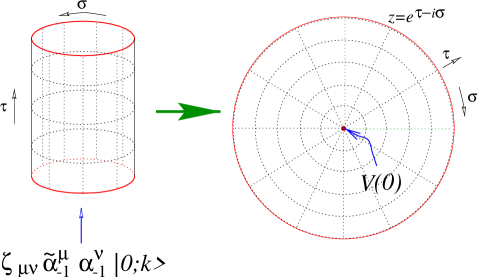
Figure 6: The correspondence between states and operator insertions. A closed string (graviton) state $\zeta_{\mu\nu}\alpha^{\mu}_{-1}{\tilde{\alpha}}^{\nu}_{-1}|0;k\!>$ is set up on the closed string at $\tau=-\infty$ and it propagates in. This is equivalent to inserting a graviton vertex operator $V^{\mu\nu}(z)=\zeta_{\mu\nu}\partial_{z}X^{\mu}\partial_{\bar{z}}X^{\nu}:e^{ik\cdot X}:$ at $z=0$.

The state with no oscillators excited (the tachyon), but with some momentum $k$, simply corresponds in this dictionary to the insertion of:

$$|0;k>\qquad\Leftrightarrow\qquad\int d^{2}z:e^{ik\cdot X}:$$ (84)

This is reasonable, as it is the simplest form that allows the right behaviour under translations: A translation by a constant vector, $X^{\mu}\to X^{\mu}+T^{\mu}$, results in a multiplication of the operator (and hence the state) by a phase $e^{ik\cdot T}$. The normal ordering signs $::$ are there to remind that the expression means to expand and keep all creation operators to the right, when expanding in terms of the $\alpha_{\pm m}$’s.

The closed string level 1 vertex operator corresponds to the emission or absorption of $G_{\mu\nu}$, $B_{\mu\nu}$ and $\Phi$:

$$\zeta_{\mu\nu}\alpha_{-1}^{\mu}{\tilde{\alpha}}_{-1}^{\nu}|0;k\!>\qquad\Leftrightarrow\qquad\int d^{2}z\,\,\zeta_{\mu\nu}\partial_{z}X^{\mu}\partial_{\bar{z}}X^{\nu}:e^{ik\cdot X}:$$ (85)

where the symmetric part of $\zeta_{\mu\nu}$ is the graviton and the antisymmetric part is the antisymmetric tensor.

More generally, in the full treatment of the string theory, where the world sheet, ${\cal M}$, is not flat but curved, the vertex operator is:

$$V={g_{s}\over\alpha^{\prime}}\int_{\cal M}d^{2}\!\sigma\,\,g^{1/2}\,\left\{(g^{ab}s_{\mu\nu}+i\epsilon^{ab}a_{\mu\nu})\partial_{a}X^{\mu}\partial_{b}X^{\nu}e^{ik\cdot X}+\alpha^{\prime}\phi Re^{ik\cdot X}\right\}\ ,$$ (86)

where $s$ is symmetric, $a$ is antisymmetric and $\phi$ is a constant, and we have put in the closed string coupling to take into account the fact that the world sheet topology changes when we emit or absorb a closed string state. A linear combination of the trace of $s$ and $\phi$ turn out to be the dilaton. The $\int d^{2}\!\sigma\,\,R$ coupling is included as a possibility simply because it is allowed by Weyl and reparametrisation invariance, as we stated earlier.

For the open string, the story is similar, but we get two copies of the relations (83) for the single set of modes $\alpha_{-n}^{\mu}$ (recall that there are no ${\tilde{\alpha}}$’s). This results in, for example the relation for the photon:

$$\zeta_{\mu}\alpha_{-1}^{\mu}|0;k\!>\qquad\Leftrightarrow\qquad\int dl\,\,\zeta_{\mu}\partial_{t}X^{\mu}:e^{ik\cdot X}:\ ,$$ (87)

where the integration is along the real line (the edge of the half–plane, which corresponds to the vertical edges of the string world-sheet on the left of figure 5. Also, $\partial_{t}$ means the derivative tangential to the boundary. The tachyon is simply the boundary insertion of the momentum $:e^{ik\cdot X}:$ alone.

The fact that the photon is associated with the ends of the string is a sort of quantum version of that which we saw in the classical analysis: That the ends of the strings move with the speed of light. Of course, we see that there are other features which we did not see in the classical analysis (like the tachyon), but our hard work in trying to retain the classical symmetries after going to the quantum case has paid off.

2.4 Chan-Paton Factors

While we are remarking upon the behaviour of the ends of the string, let us endow them with a slightly more interesting property. We can add non-dynamical degrees of freedom to the ends of the string without spoiling spacetime Poincaré invariance or world–sheet conformal invariance. These are called “Chan–Paton” degrees of freedom and by declaring that their Hamiltonian is zero, we guarantee that they stay in the state that we put them in. In addition to the usual Fock space labels we have been using for the state of the string, we ask that each end be in a state $i$ or $j$ for $i,j$ from $1$ to $N$ (see figure 7).

Figure 7: An open string with Chan–Paton degrees of freedom.

We use a family of $N\times N$ matrices, $\lambda^{a}_{ij}$, as a basis into which to decompose a string wavefunction

$$|k;a\rangle=\sum^{N}_{i,j=1}|k,ij\rangle\lambda^{a}_{ij}.$$ (88)

These wavefunctions are called “Chan-Paton factors”[20]. Similarly, all open string vertex operators carry such factors. For example, consider the tree–level (disc) diagram for the interaction of four oriented open strings in figure 8.

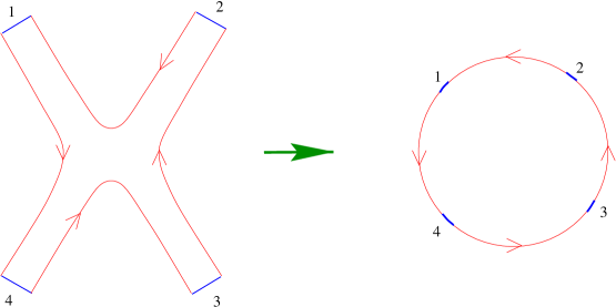
Figure 8: A four–point Scattering of open strings, and its conformally related disc amplitude.

As the Chan–Paton degrees of freedom are non-dynamical, the right end of string #1 must be in the same state as the left end of string #2, etc., as we go around the edge of the disc. After summing over all the possible states involved in tying up the ends, we are left with a trace of the product of Chan–Paton factors,

$$\lambda^{1}_{ij}\lambda^{2}_{jk}\lambda^{3}_{kl}\lambda^{4}_{li}={\rm Tr}(\lambda^{1}\lambda^{2}\lambda^{3}\lambda^{4}).$$ (89)

All open string amplitudes will have a trace like this and are invariant under a global (on the world–sheet) $U(N)$: 

$$\lambda^{i}\ \to\ U\lambda^{i}U^{-1},$$ (90)

under which the endpoints transform as $\mathbf{N}$ and $\bar{\mathbf{N}}$.

Notice that the massless vector vertex operator $V^{a\mu}=\lambda^{a}_{ij}\partial_{t}X^{\mu}\exp(ik\cdot X)$ transforms as the adjoint under the $U(N)$ symmetry. This means that the global symmetry of the world-sheet theory is promoted to a gauge symmetry in spacetime. It is a gauge symmetry because we can make a different $U(N)$ rotation at separate points $X^{\mu}(\sigma,\tau)$ in spacetime.

2.5 The Closed String Partition Function

We have all of the ingredients we need to compute our first one–loop diagram. It will be useful to do this as a warm up for more complicated examples later, and in fact we will see structures in this simple case which will persist throughout.

Consider the closed string diagram of figure 9(a). This is a vacuum diagram, since there are no external strings. This torus is clearly a one loop diagram and in fact it is easily computed. It is distinguished topologically by having two completely independent one–cycles. To compute the path integral for this we are instructed, as we have seen, to sum over all possible metrics representing all possible surfaces, and hence all possible tori.

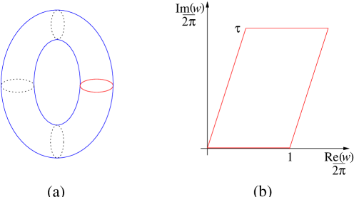
Figure 9: (a) A closed string vacuum diagram (b). The flat torus and its complex structure.

Well, the torus is completely specified by giving it a flat metric, and a complex structure, $\tau$, with ${\rm Im}\tau\geq 0$. It can be described by the lattice given by quotienting the complex $w$–plane by the equivalence relations

$$w\sim w+2\pi n\ ;\quad w\sim w+2\pi m\tau\ ,$$ (91)

for any integers $m$ and $n$, as shown in figure 9(b). The two one–cycles can be chosen to be horizontal and vertical. The complex number $\tau$ specifies the shape of a torus, which cannot be changed by infinitesimal diffeomorphisms of the metric, and so we must sum over all all of them. Actually, this naive reasoning will make us overcount by a lot, since in fact there are a lot of $\tau$’s which define the same torus. For example, clearly for a torus with given value of $\tau$, the torus with $\tau+1$ is the same torus, by the equivalence relation (91). The full family of equivalent tori can be reached from any $\tau$ by the “modular transformations”:

$$T :\quad\tau\to\tau+1$$ (92)

$$S :\quad\tau\to-{1\over\tau}\ ,$$

which generate the group $SL(2,{\hbox{{\rm Z}\kern-3.99994pt\hbox{\rm Z}}})$, which is represented here as the group of $2\times 2$ unit determinant matrices with integer elements:

$$SL(2,{\hbox{{\rm Z}\kern-3.99994pt\hbox{\rm Z}}}):\quad\tau\to{a\tau+b\over c\tau+d}\ ;\quad\mbox{with}\quad\pmatrix{a&b\cr c&d}\ ,\quad ad-bc=1\ .$$ (93)

(It is worth noting that the map between tori defined by $S$ exchanges the two one–cycles, therefore exchanging space and (Euclidean) time.) The full family of inequivalent tori is given not by the upper half plane $H_{\perp}$ (i.e., $\tau$ such that ${\rm Im}\tau\geq 0$) but the quotient of it by the equivalence relation generated by the group of modular transformations. This is ${\cal F}=H_{\perp}/PSL(2,{\hbox{{\rm Z}\kern-3.99994pt\hbox{\rm Z}}})$, where the $P$ reminds us that we divide by the extra ${\hbox{{\rm Z}\kern-3.99994pt\hbox{\rm Z}}}_{2}$ which swaps the sign on the defining $SL(2,{\hbox{{\rm Z}\kern-3.99994pt\hbox{\rm Z}}})$ matrix, which clearly does not give a new torus. The commonly used fundamental domain in the upper half plane corresponding to the inequivalent tori is drawn in figure 10. Any point outside that can be mapped into it by a modular transformation.

Figure 10: The space of inequivalent tori is blue.

The string propagation on our torus can be described as follows. Imagine that the string is of length 1, and lies horizontally. Mark a point on the string. Running time upwards, we see that the string propagates for a time $t=2\pi{\rm Im}\tau\equiv 2\pi\tau_{2}$. One it has got to the top of the diagram, we see that our marked point has shifted rightwards by an amount $x=2\pi{\rm Re}\tau\equiv 2\pi\tau_{1}$. We actually already have studied the operators which perform these two operations. The operator for time translations is the Hamiltonian (63), $H=L_{0}+{\bar{L}}_{0}-({{\rm c}+{\bar{\rm c}}})/24$ while the operator for translations along the string is the momentum $P=L_{0}-{\bar{L}}_{0}$ discussed above eqn.(72). Recall that ${\rm c}={\bar{\rm c}}{=}D{-}2{=}24$. So our vacuum path integral is

$$Z={\rm Tr}\left\{e^{-2\pi\tau_{2}H}e^{2\pi{\rm i}\tau_{1}P}\right\}={\rm Tr}q^{L_{0}-{c\over 24}}{\bar{q}}^{{\bar{L}}_{0}-{{\bar{c}}\over 24}}\ .$$ (94)

Here, $q\equiv e^{2\pi{\rm i}\tau}$, and the trace means a sum over everything which is discrete and an integral over everything which is continuous, which in this case, is simply $\tau$. This is easily evaluated, as the expressions for $L_{0}$ and ${\bar{L}}_{0}$ give a family of simple geometric sums (see insert 4 (p.2.5)), and the result can be written as:

$$Z=\int_{\cal F}{d^{2}\tau\over\tau_{2}}Z(q)\ ,\quad\mbox{where}$$ (95)

$$Z(q)=|\tau_{2}|^{-12}(q{\bar{q}})^{-1}\left|\prod_{n=1}^{\infty}\left(1-q^{n}\right)^{-24}\right|^{2}=\left(\sqrt{\tau_{2}}\eta{\bar{\eta}}\right)^{-24}\ ,$$ (96)

is the “partition function”, with Dedekind’s function

$$\eta(q)\equiv q^{1\over 24}\prod_{n=1}^{\infty}\left(1-q^{n}\right)\ ;\quad\eta\left(-{1\over\tau}\right)=\sqrt{-{\rm i}\tau}\,\eta(\tau)\ .$$ (97)

Insert 4: Partition Functions It is not hard to do the sums. Let us look at one dimension, and so one family of oscillators $\alpha_{n}$. We need to consider $${\rm Tr}\,q^{L_{0}}={\rm Tr}\,q^{\sum_{n=0}^{\infty}\alpha_{-n}\alpha_{n}}\ .$$ We can see what the operator $q^{\sum_{n=0}^{\infty}\alpha_{-n}\alpha_{n}}$ means if we write it explicitly in a basis of all possible multiparticle states of the form $\alpha_{-n}|0\!>$, $(\alpha_{-n})^{2}|0\!>$, etc. : $$q^{\alpha_{-n}\alpha_{n}}=\pmatrix{1&&&&\cr&q^{n}&&&\cr&&q^{2n}&&\cr&&&q^{3n}&\cr&&&&\ddots\cr}\ ,$$ and so clearly ${\rm Tr}q^{\alpha_{-n}\alpha_{n}}=\sum_{i=1}^{\infty}(q^{n})^{i}=(1-q^{n})^{-1}$, which is remarkably simple! The final sum over all modes is trivial, since $${\rm Tr}\,q^{\sum_{n=0}^{\infty}\alpha_{-n}\alpha_{n}}=\prod_{n=0}^{\infty}{\rm Tr}\,q^{\alpha_{-n}\alpha_{n}}=\prod_{n=0}^{\infty}(1-q^{n})^{-1}\ .$$ We get a factor like this for all 24 dimensions, and we also get contributions from both the left and right to give the result. Notice that if our modes were fermions, $\psi_{n}$, things would be even simpler. We would not be able to make multiparticle states $(\psi_{-n})^{2}|0\!>$, (Pauli), and so we only have a $2{\times}2$ matrix of states to trace in this case, and so we simply get $${\rm Tr}\,q^{\psi_{-n}\psi_{n}}=(1+q^{n})\ .$$ Therefore the partition function is $${\rm Tr}\,q^{\sum_{n=0}^{\infty}\psi_{-n}\psi_{n}}=\prod_{n=0}^{\infty}{\rm Tr}q^{\psi_{-n}\psi_{n}}=\prod_{n=0}^{\infty}(1+q^{n})\ .$$ We will encounter such fermionic cases later.

This is a pleasingly simple result. One very interesting property it has is that it is actually “modular invariant”. It is invariant under the $T$ transformation in (91), since under $\tau\to\tau+1$, we get that $Z(q)$ picks up a factor $\exp(2\pi{\rm i}(L_{0}-{\bar{L}}_{0}))$. This factor is precisely unity, as follows from the level matching formula (72). Invariance of $Z(q)$ under the $S$ transformation $\tau\to-1/\tau$ follows from the property mentioned in (97), after a few steps of algebra, and using the result $S:\,\,\tau_{2}\to\tau_{2}/|\tau|^{2}$.

Modular invariance of the partition function is a crucial property. It means that we are correctly integrating over all inequivalent tori, which is required of us by diffeomorphism invariance of the original construction. Furthermore, we are counting each torus only once, which is of course important.

Note that $Z(q)$ really deserves the name “partition function” since if it is expanded in powers of $q$ and $\bar{q}$, the powers in the expansion —after multiplication by $4/\alpha^{\prime}$— refer to the (mass)² level of excitations on the left and right, while the coeeficient in the expansion gives the degeneracy at that level. The degeneracy is the number of partitions of the level number into positive integers. For example, at level 3 this is 3, since we have $\alpha_{-3},\alpha_{-1}\alpha_{-2}$, and $\alpha_{-1}\alpha_{-1}\alpha_{-1}$.

The overall factor of $(q{\bar{q}})^{-1}$ sets the bottom of the tower of masses. Note for example that at level zero we have the tachyon, which appears only once, as it should, with $M^{2}=-4/\alpha^{\prime}$. At level one, we have the massless states, with multiplicity $24^{2}$, which is appropriate, since there are $24^{2}$ physical states in the graviton multiplet $(G_{\mu\nu},B_{\mu\nu},\Phi)$. Introducing a common piece of terminology, a term $q^{w_{1}}{\bar{q}}^{w_{2}}$, represents the appearance of a “weight” $(w_{1},w_{2})$ field in the 1+1 dimensional conformal field theory, denoting its left–moving and right–moving weights or “conformal dimensions”.

2.6 Unoriented Strings

$\bullet\quad{\mbox{\it Unoriented Open Strings}}$

There is an operation of world sheet parity $\Omega$ which takes $\sigma\to\pi-\sigma$, on the open string, and acts on $z=e^{\tau-i\sigma}$ as $z\leftrightarrow-\bar{z}$. In terms of the mode expansion (80), $X^{\mu}(z,\bar{z})\to X^{\mu}(-\bar{z},-z)$ yields

$$x^{\mu} \rightarrow x^{\mu}$$

$$p^{\mu} \rightarrow p^{\mu}$$

$$\alpha^{\mu}_{m} \rightarrow (-1)^{m}\alpha^{\mu}_{m}\ .$$ (98)

This is a global symmetry of the open string theory and so, we can if we wish also consider the theory that results when it is gauged, by which we mean that only $\Omega$–invariant states are left in the spectrum. We must also consider the case when we take a string around a closed loop, it is allowed to come back to itself only up to an over all action of $\Omega$, which is to swap the ends. This means that we must include unoriented worldsheets in our analysis. For open strings, the case of the Möbius strip is a useful example to keep in mind. It is on the same footing as the cylinder when we consider gauging $\Omega$. The string theories which result from gauging $\Omega$ are understandably called “unoriented string theories”.

Let us see what becomes of the string spectrum when we perform this projection. The open string tachyon is even under $\Omega$ and so survives the projection. However, the photon, which has only one oscillator acting, does not:

$$\Omega|{k}\rangle = +|{k}\rangle$$

$$\Omega\alpha^{\mu}_{-1}|{k}\rangle = -\alpha^{\mu}_{-1}|{k}\rangle.$$ (99)

We have implicitly made a choice about the sign of $\Omega$ as it acts on the vacuum The choice we have made in writing eqn. (99) corresponds to the symmetry of the vertex operators (87): the resulting minus sign comes from the orientation reversal on the tangent derivative $\partial_{t}$ (see figure 11).

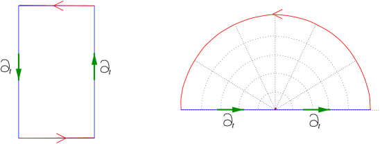
Figure 11: The action of $\Omega$ on the photon vertex operator can be deduced from seeing how exchanging the ends of the string changes the sign of the tangent derivative, $\partial_{t}$.

Fortunately, we have endowed the string’s ends with Chan–Paton factors, and so there is some additional structure which can save the photon. While $\Omega$ reverses the Chan–Paton factors on the two ends of the string, it can have some additional action:

$$\Omega\lambda_{ij}|{k},ij\rangle\ \to\ \lambda^{\prime}_{ij}|{k},ij\rangle,\quad\lambda^{\prime}=M\lambda^{T}M^{-1}.$$ (100)

This form of the action on the Chan–Paton factor follows from the requirement that it be a symmetry of the amplitudes which have factors like those in eqn. (89).

If we act twice with $\Omega$, this should square to the identity on the fields, and leave only the action on the Chan–Paton degrees of freedom. States should therefore be invariant under:

$$\lambda\to MM^{-T}\lambda M^{T}M^{-1}.$$ (101)

Now it should be clear that the $\lambda$ must span a complete set of $N\times N$ matrices: If strings with ends labelled $ik$ and $jl$ are in the spectrum for any values of $k$ and $l$, then so is the state $ij$. This is because $jl$ implies $lj$ by CPT, and a splitting–joining interaction in the middle gives $ik+lj\to ij+lk$.

Now equation (101) and Schur’s lemma require $MM^{-T}$ to be proportional to the identity, so $M$ is either symmetric or antisymmetric. This gives two distinct cases, modulo a choice of basis. Denoting the $n\times n$ unit matrix as $I_{n}$, we have [22] the symmetric case:

$$\qquad\ M=M^{T}=I_{N}$$ (102)

In order for the photon $\lambda_{ij}\alpha^{\mu}_{-1}|{k}\rangle$ to be even under $\Omega$ and thus survive the projection, $\lambda$ must be antisymmetric to cancel the minus sign from the transformation of the oscillator state. So $\lambda=-\lambda^{T}$, giving the gauge group $SO(N)$. For the antisymmetric case, we have:

$$M=-M^{T}=i\left[\begin{array}[]{cc}0&I_{N/2}\\ -I_{N/2}&0\end{array}\right]$$ (103)

For the photon to survive, $\lambda=-M\lambda^{T}M$, which is the definition of the gauge group $USp(N)$. Here, we use the notation that $USp(2)\equiv SU(2)$. Elsewhere in the literature this group is often denoted $Sp(N/2)$.

$\bullet\quad{\mbox{\it Unoriented Closed Strings}}$

Turning to the closed string sector. For closed strings, we see that the mode expansion (81) for $X^{\mu}(z,\bar{z})=X^{\mu}_{L}(z)+X^{\mu}_{R}(\bar{z})$ is invariant under a world–sheet parity symmetry $\sigma\to-\sigma$, which is $z\to-\bar{z}$. (We should note that this is a little different from the choice of $\Omega$ we took for the open strings, but more natural for this case. The two choices are related to other by a shift of $\pi$.) This natural action of $\Omega$ simply reverses the left– and right–moving oscillators:

$$\Omega\colon\qquad\alpha^{\mu}_{n}\leftrightarrow{\tilde{\alpha}}^{\mu}_{n}.$$ (104)

Let us again gauge this symmetry, projecting out the states which are odd under it. Once again, since the tachyon contains no oscillators, it is even and is in the projected spectrum. For the level 1 excitations:

$$\Omega\alpha^{\mu}_{-1}{\tilde{\alpha}}^{\nu}_{-1}|k\rangle={\tilde{\alpha}}^{\mu}_{-1}\alpha^{\nu}_{-1}|k\rangle,$$ (105)

and therefore it is only those states which are symmetric under $\mu\leftrightarrow\nu$ —the graviton and dilaton— which survive the projection. The antisymmetric tensor is projected out of the theory.

$\bullet\quad{\mbox{\it Worldsheet Diagrams}}$

As stated before, once we have gauged $\Omega$, we must allow for unoriented worldsheets, and this gives us rather more types of string worldsheet than we have studied so far. Figure 12 depicts the two types of one–loop diagram we must consider when computing amplitudes for the open string. The annulus (or cylinder) is on the left, and can be taken to represent an open string going around in a loop. The Möbius strip on the right is an open string going around a loop, but returning with the ends reversed. The two surfaces are constructed by identifying a pair of opposite edges on a rectangle, one with and the other without a twist.

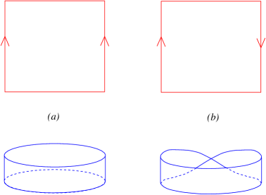
Figure 12: (a) Constructing a cylinder or annulus by identifying a pair of opposite edges of a rectangle. (b) Constructing a Möbius strip by identifying after a twist.

Figure 13 shows an example of two types of closed string one–loop diagram we must consider. On the left is a torus, while on the right is a Klein bottle, which is constructed in a similar way to a torus save for a twist introduced when identifying a pair of edges.

Figure 13: (a) Constructing a torus by identifying opposite edges of a rectangle. (b) Constructing a Klein bottle by identifying after a twist.

In both the open and closed string cases, the two diagrams can be thought of as descending from the oriented case after the insertion of the normalised projection operator ${1\over 2}{\rm Tr}(1+\Omega)$ into one–loop amplitudes.

Similarly, the unoriented one-loop open string amplitude comes from the annulus and Möbius strip. We will discuss these amplitudes in more detail later.

The lowest order unoriented amplitude is the projective plane $\mathbf{RP}^{2}$, which is a disk with opposite points identified.

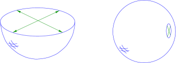
Figure 14: Constructing the projective plane $\mathbf{RP}^{2}$ by identifying opposite points on the disk. This is equivalent to a sphere with a crosscap insertion.

Shrinking the identified hole down, we recover the fact that $\mathbf{RP}^{2}$ may be thought of as a sphere with a crosscap inserted, where the crosscap is the result of shrinking the identified hole. Actually, a Möbius strip can be thought of as a disc with a crosscap inserted, and a Klein Bottle is a sphere with two crosscaps. Since a sphere with a hole (one boundary) is the same as a disc, and a sphere with one handle is a torus, we can classify all world sheet diagrams in terms of the number of handles, boundaries and crosscaps that they have. Insert 5 (p.2.6) summaries all the world sheet perturbation theory diagrams up to one loop.

Insert 5: World Sheet Perturbation Theory: Diagrammatics It is worthwhile summarising all of the string theory diagrams up to one–loop in a table. Recall that each diagram is weighted by a factor $g_{s}^{\chi}=g_{s}^{2h-2+b+c}$ where $h,b,c$ are the numbers of handles, boundaries and crosscaps, respectively.

$g_{s}^{-2}$ $g_{s}^{-1}$ $g_{s}^{0}$ $\matrix{\mbox{closed}\cr\mbox{oriented}}$ $\matrix{\cr\mbox{sphere $S^{2}$}\cr\mbox{(plane)}\cr\psfig{height=57.81621pt}}$ $\cdot$ $\matrix{\cr\mbox{torus $T^{2}$}\cr\cr\psfig{height=57.81621pt}}$ $\matrix{\mbox{open}\cr\mbox{oriented}}$ $\cdot$ $\matrix{\cr\mbox{disc $D_{2}$}\cr\mbox{(half--plane)}\cr\psfig{height=57.81621pt}}$ $\matrix{\cr\mbox{cylinder $C_{2}$}\cr\mbox{(annulus)}\cr\psfig{height=57.81621pt}}$ $\matrix{\mbox{closed}\cr\mbox{unoriented}}$ $\cdot$ $\matrix{\mbox{projective}\cr\mbox{plane }\mathbf{RP}^{2}\cr\cr\psfig{height=57.81621pt}}$ $\matrix{\cr\mbox{Klein Bottle KB}\cr\cr\psfig{height=57.81621pt}}$ $\matrix{\mbox{open}\cr\mbox{unoriented}}$ $\cdot$ $\cdot$ $\matrix{\cr\mbox{M\"{o}bius Strip MS}\cr\cr\psfig{height=57.81621pt}}$

2.7 Strings in Curved Backgrounds

So far, we have studied strings propagating in the (uncompactified) target spacetime with metric $\eta_{\mu\nu}$. While this alone is interesting, it is curved backgrounds of one sort or another which will occupy much of this school, and so we ought to see how they fit into the framework so far.

A natural generalisation of our action is simply to study the “sigma model” action:

$$S_{\sigma}=-{1\over 4\pi\alpha^{\prime}}\int d^{2}\!\sigma\,(-g)^{1/2}g^{ab}G_{\mu\nu}(X)\partial_{a}X^{\mu}\partial_{b}X^{\nu}\ .$$ (106)

Comparing this to what we had before (20), we see that from the two dimensional point of view this still looks like a model of $D$ bosonic fields $X^{\mu}$, but with field dependent couplings given by the non–trivial spacetime metric $G_{\mu\nu}(X)$. This is an interesting action to study.

A first objection to this is that we seem to have cheated somewhat: Strings are supposed to generate the graviton (and ultimately any curved backgrounds) dynamically. Have we cheated by putting in such a background by hand? Or a more careful, less confrontational question might be: Is it consistent with the way strings generate the graviton to introduce curved backgrounds in this way?

Well, let us see. Imagine, to start off, that the background metric is only locally a small deviation from flat space: $G_{\mu\nu}(X)=\eta_{\mu\nu}+h_{\mu\nu}(X)$, where $h$ is small.

Then, in conformal gauge, we can write in the Euclidean path integral (35):

$$e^{-S_{\sigma}}=e^{-S}\left(1+{1\over 4\pi\alpha^{\prime}}\int d^{2}zh_{\mu\nu}(X)\partial_{z}X^{\mu}\partial_{\bar{z}}X^{\nu}+\ldots\right)\ ,$$ (107)

and we see that if $h_{\mu\nu}(X)\propto g_{s}\zeta_{\mu\nu}\exp(ik\cdot X)$, where $\zeta$ is a symmetric polarisation matrix, we are simply inserting a graviton emission vertex operator. So we are indeed consistent with that which we have already learned about how the graviton arises in string theory. Furthermore, the insertion of the full $G_{\mu\nu}(X)$ is equivalent in this language to inserting an exponential of the graviton vertex operator, which is another way of saying that a curved background is a “coherent state” of gravitons.

It is clear that we should generalise our success, by including sigma model couplings which correspond to introducing background fields for the antisymmetric tensor and the dilaton, mimicking (86):

$$S_{\sigma}={1\over 4\pi\alpha^{\prime}}\int d^{2}\!\sigma\,g^{1/2}\,\left\{(g^{ab}G_{\mu\nu}(X)+i\epsilon^{ab}B_{\mu\nu}(X))\partial_{a}X^{\mu}\partial_{b}X^{\nu}+\alpha^{\prime}\Phi R\right\}\ ,$$ (108)

where $B_{\mu\nu}$ is the background antisymmetric tensor field and $\Phi$ is the background value of the dilaton. The next step is to do a full analysis of this new action and ensure that in the quantum theory, one has Weyl invariance, which amounts to the tracelessness of the two dimensional stress tensor. Calculations (which we will not discuss here) reveal that: [1, 5]

$$T^{a}_{\phantom{a}a}=-{1\over 2\alpha^{\prime}}\beta_{\mu\nu}^{G}g^{ab}\partial_{a}X^{\mu}\partial_{b}X^{\nu}-{i\over 2\alpha^{\prime}}\beta_{\mu\nu}^{B}\epsilon^{ab}\partial_{a}X^{\mu}\partial_{b}X^{\nu}-{1\over 2}\beta^{\Phi}R\ .$$ (109)

with

$$\beta_{\mu\nu}^{G} = \alpha^{\prime}\left(R_{\mu\nu}+2\nabla_{\mu}\nabla_{\nu}\Phi-{1\over 4}H_{\mu\kappa\sigma}H_{\nu}^{\phantom{\nu}\kappa\sigma}\right)+O(\alpha^{\prime 2}),$$

$$\beta_{\mu\nu}^{B} = \alpha^{\prime}\left(-{1\over 2}\nabla^{\kappa}H_{\kappa\mu\nu}+\nabla^{\kappa}\Phi H_{\kappa\mu\nu}\right)+O(\alpha^{\prime 2}),$$

$$\beta^{\Phi} = \alpha^{\prime}\left({D-26\over 6\alpha^{\prime}}-{1\over 2}\nabla^{2}\Phi+\nabla_{\kappa}\Phi\nabla^{\kappa}\Phi-{1\over 24}H_{\kappa\mu\nu}H^{\kappa\mu\nu}\right)+O(\alpha^{\prime 2})\ ,$$ (110)

with $H_{\mu\nu\kappa}\equiv\partial_{\mu}B_{\nu\kappa}+\partial_{\nu}B_{\kappa\mu}+\partial_{\kappa}B_{\mu\nu}.$ For Weyl invariance, we ask that each of these beta functions for the sigma model couplings actually vanish. The remarkable thing is that these resemble spacetime field equations for the background fields. In fact, the field equations can be derived from the following spacetime action:

$${\rm S} = {1\over 2\kappa^{2}_{0}}\int d^{D}X(-G)^{1/2}e^{-2\Phi}\left[R+4\nabla_{\mu}\Phi\nabla^{\mu}\Phi-{1\over 12}H_{\mu\nu\lambda}H^{\mu\nu\lambda}\right.$$ (111)

$$\hskip 142.26378pt\left.-{2(D-26)\over 3\alpha^{\prime}}+O(\alpha^{\prime})\right]\ .$$

N.B.: Now we note something marvellous: $\Phi$ is a background field which appears in the closed string theory sigma model multiplied by the Euler density. So comparing to (34) (and discussion following), we recover the remarkable fact that the string coupling $g_{s}$ is not fixed, but is in fact given by the value of one of the background fields in the theory: $g_{s}=e^{<\Phi>}$. So the only free parameter in the theory is the string tension.

Turning to the open string sector, we may also write the effective action which summarises the leading order (in $\alpha^{\prime}$) open string physics at tree level:

$${\rm S}=-{{\rm C}\over 4}\int d^{D}X\,e^{-\Phi}{\rm Tr}F_{\mu\nu}F^{\mu\nu}+O(\alpha^{\prime})\ ,$$ (112)

with ${\rm C}$ a dimensionful constant which we will fix later. It is of course of the form of the Yang–Mills action, where $F_{\mu\nu}=\partial_{\mu}A_{\nu}-\partial_{\nu}A_{\mu}$. The field $A_{\mu}$ is coupled in sigma–model fashion to the boundary of the world sheet by the boundary action:

$$\int_{\partial{\cal M}}d\tau\,A_{\mu}\partial_{t}X^{\mu}\ ,$$ (113)

mimicking the form of the vertex operator (87).

One should note the powers of $e^{\Phi}$ in the above actions. Recall that the expectation value of $e^{\Phi}$ sets the value of $g_{s}$. We see that the appearance of $\Phi$ in the actions are consistent with this, as we have $e^{-2\Phi}$ in front of all of the closed string parts, representing the sphere ($g_{s}^{-2}$) and $e^{-\Phi}$ for the open string, representing the disc ($g_{s}^{-1}$).

Notice that if we make the following redefinition of the background fields:

$${\tilde{G}}_{\mu\nu}(X)=e^{2\Omega(X)}G_{\mu\nu}=e^{4(\Phi_{0}-\Phi)/(D-2)}G_{\mu\nu}\ ,$$ (114)

and use the fact that the new Ricci scalar can be derived using:

$${\tilde{R}}=e^{-2\Omega}\left[R-2(D-1)\nabla^{2}\Omega-(D-2)(D-1)\partial_{\mu}\Omega\partial^{\mu}\Omega\right]\ ,$$ (115)

The action (111) becomes:

$${\rm S} = {1\over 2\kappa^{2}}\int d^{D}X(-{\tilde{G}})^{1/2}\left[R-{4\over D-2}\nabla_{\mu}{\tilde{\Phi}}\nabla^{\mu}{\tilde{\Phi}}-{1\over 12}e^{-8{\tilde{\Phi}}/(D-2)}H_{\mu\nu\lambda}H^{\mu\nu\lambda}\right.$$

$$\hskip 156.49014pt\left.-{2(D-26)\over 3\alpha^{\prime}}e^{4{\tilde{\Phi}}/(D-2)}+O(\alpha^{\prime})\right]\ ,$$

with ${\tilde{\Phi}}=\Phi-\Phi_{0}$, Looking at the part involving the Ricci scalar, we see that we have the form of the standard Einstein–Hilbert action (i.e., we have removed the factor involving the dilaton $\Phi$), with Newton’s constant set by

$$\kappa\equiv\kappa_{0}e^{\Phi_{0}}=(8\pi G_{N})^{1/2}\ .$$ (117)

The standard terminology to note here is that the action (111) written in terms of the original fields is called the “string frame”, while the action (LABEL:einsteinfrm) is referred to as the “Einstein frame” action. It is in the latter frame that one gives meaning to measuring quantities like gravitational mass–energy. It is important to note the means to transform from the fields of one to another, depending upon dimension (114). See also the supersymmetric cases much later in these notes.

3 Target Spacetime Perspective, Mostly

In this section we shall study T–duality. [12] This is very dramatic symmetry of the theory of strings under a spacetime transformation. It is a crucial consequence of the fact that strings are extended objects.

3.1 T–Duality for Closed Strings

Let us start with closed strings, first focusing on the zero modes. The mode expansion (81) can be written:

$$X^{\mu}(z,\bar{z})=x^{\mu}+\tilde{x}^{\mu}-i\sqrt{{\alpha^{\prime}}\over 2}(\alpha^{\mu}_{0}+{\tilde{\alpha}}^{\mu}_{0})\tau+\sqrt{{\alpha^{\prime}}\over 2}(\alpha^{\mu}_{0}-{\tilde{\alpha}}^{\mu}_{0})\sigma+{\rm oscillators}.$$ (118)

We have already identified the spacetime momentum of the string:

$$p^{\mu}={1\over{\sqrt{2{\alpha^{\prime}}}}}(\alpha^{\mu}_{0}+{\tilde{\alpha}}^{\mu}_{0})\ .$$ (119)

If we run around the string, i.e., take $\sigma\to\sigma+2\pi$, the oscillator term are periodic and we have

$$X^{\mu}(z,\bar{z})\to X^{\mu}(z,\bar{z})+2\pi\sqrt{\alpha^{\prime}\over 2}(\alpha^{\mu}_{0}-{\tilde{\alpha}}^{\mu}_{0})\ .$$ (120)

So far, we have studied the situation of non–compact spatial directions for which the embedding function $X^{\mu}(z,\bar{z})$ is single–valued, and therefore the above change must be zero, giving

$$\alpha^{\mu}_{0}={\tilde{\alpha}}^{\mu}_{0}=\sqrt{{\alpha^{\prime}}\over 2}p^{\mu}.$$ (121)

Momentum $P^{\mu}$ takes a continuum of values reflecting the fact that the direction $X^{\mu}$ is non–compact.

Let us consider the case that we have a compact direction, say $X^{25}$, of radius $R$. Our direction $X^{25}$ therefore has period $2\pi R$. The momentum $p^{25}$ now takes the discrete values $n/R$, for $n\in{\hbox{{\rm Z}\kern-3.99994pt\hbox{\rm Z}}}$. Now, under $\sigma\sim\sigma+2\pi$, $X^{25}(z,\bar{z})$ is not single valued, and can change by $2\pi wR$, for $w\in{\hbox{{\rm Z}\kern-3.99994pt\hbox{\rm Z}}}$. Solving the two resulting equations gives:

$$\alpha^{25}_{0}+{\tilde{\alpha}}^{25}_{0} = {2n\over R}\sqrt{{\alpha^{\prime}}\over 2}$$

$$\alpha^{25}_{0}-{\tilde{\alpha}}^{25}_{0} = \sqrt{2\over{\alpha^{\prime}}}wR$$ (122)

and so we have:

$$\alpha^{25}_{0} = \left({n\over R}+{wR\over{\alpha^{\prime}}}\right)\sqrt{{\alpha^{\prime}}\over 2}\equiv P_{L}\sqrt{{\alpha^{\prime}}\over 2}$$

$${\tilde{\alpha}}^{25}_{0} = \left({n\over R}-{wR\over{\alpha^{\prime}}}\right)\sqrt{{\alpha^{\prime}}\over 2}\equiv P_{R}\sqrt{{\alpha^{\prime}}\over 2}\ .$$ (123)

We can use this to compute the formula for the mass spectrum in the remaining uncompactified 24+1 dimensions, using the fact that $M^{2}=-p_{\mu}p^{\mu}$, where now $\mu=0,\ldots,24$.

$$M^{2}\ =\ -p^{\mu}p_{\mu} = {2\over{\alpha^{\prime}}}(\alpha_{0}^{25})^{2}+{4\over{\alpha^{\prime}}}({N}-1)$$ (124)

$$= {2\over{\alpha^{\prime}}}({\tilde{\alpha}}_{0}^{25})^{2}+{4\over{\alpha^{\prime}}}({\bar{N}}-1)\ ,$$

where $N,\bar{N}$ denote the total levels on the left– and right–moving sides, as before. These equations follow from the left and right $L_{0},{\bar{L}}_{0}$ constraints. Recall that the sum and difference of these give the Hamiltonian and the level–matching formulae. Here, they are modified, and a quick computation gives:

$$M^{2}={n^{2}\over R^{2}}+{w^{2}R^{2}\over\alpha^{\prime 2}}+{2\over\alpha^{\prime}}\left(N+{\tilde{N}}-2\right)$$

$$nw+N-{\tilde{N}}=0\ .$$ (125)

The key features here are that there are terms in addition to the usual oscillator contributions. In the mass formula, there is a term giving the contribution of the Kaluza–Klein tower of momentum states for the string, and a term from the tower of winding states. This latter term is a very stringy phenomenon. Notice that the level matching term now also allows a mismatch between the number of left and right oscillators excited, in the presence of discrete winding and momenta.

In fact, notice that we can get our usual massless states by taking

$$n=w=0\ ;\qquad N={\bar{N}}=1\ .$$ (126)

If we write these states out(and the corresponding fields and vertex operators, for completeness), we have:

field	state	operator
$G_{\mu\nu}$	$(\alpha^{\mu}_{-1}{\tilde{\alpha}}^{\nu}_{-1}+\alpha^{\nu}_{-1}{\tilde{\alpha}}^{\mu}_{-1})|0;k\!>$	$\partial X^{\mu}{\bar{\partial}}X^{\nu}+\partial X^{\mu}{\bar{\partial}}X^{\nu}$
$B_{\mu\nu}$	$(\alpha^{\mu}_{-1}{\tilde{\alpha}}^{\nu}_{-1}-\alpha^{\nu}_{-1}{\tilde{\alpha}}^{\mu}_{-1})|0;k\!>$	$\partial X^{\mu}{\bar{\partial}}X^{\nu}-\partial X^{\mu}{\bar{\partial}}X^{\nu}$
$A_{\mu(R)}$	$\alpha^{\mu}_{-1}{\tilde{\alpha}}^{25}_{-1}|0;k\!>$	$\partial X^{\mu}{\bar{\partial}}X^{25}$
$A_{\mu(L)}$	${\tilde{\alpha}}^{\mu}_{-1}\alpha^{25}_{-1}|0;k\!>$	$\partial X^{25}{\bar{\partial}}X^{\mu}$
$\phi\equiv G_{25,25}$	$\alpha^{25}_{-1}{\tilde{\alpha}}^{25}_{-1}|0;k\!>$	$\partial X^{25}{\bar{\partial}}X^{25}$

where

$$A_{\mu(R)}\equiv{1\over 2}(G-B)_{\mu,25}\ ;\quad A_{\mu(L)}\equiv{1\over 2}(G+B)_{\mu,25}\ .$$

(we have listed the zero momentum vertex operators for these states also).

These 25 dimensional massless states are basically the components of the graviton and antisymmetric tensor fields in 26 dimensions, now relabelled. (There is also of course the dilaton $\Phi$, which we have not listed.) There is a pair of gauge fields giving a $U(1)_{L}{\times}U(1)_{R}$ gauge symmetry, and in addition a massless scalar field $\phi$. Actually, $\phi$ is a massless scalar which can have any background vacuum expectation value (vev), which in fact sets the radius of the circle. This is because the square root of the metric component $G_{25,25}$ is indeed the measure of the radius of the $X^{25}$ direction.

Let us now study the generic behaviour of the spectrum (125) for different values of $R$. For larger and larger $R$, momentum states become lighter, and therefore it is less costly to excite them in the spectrum. At the same time, winding states become heavier, and are more costly. For smaller and smaller $R$, the reverse is true, and it is gets cheaper to excite winding states and it is momentum states which become more costly.

We can take this further: As $R\to\infty$, all of the winding states i.e., states with $w\neq 0$, become infinitely massive, while the $w=0$ states with all values of $n$ go over to a continuum. This fits with what we expect intuitively, and we recover the fully uncompactified result.

Consider instead the case $R\to 0$, where all of the momentum states i.e., states with $n\neq 0$, become infinitely massive. If we were studying field theory we would stop here, as this would be all that would happen—the surviving fields would simply be independent of the compact coordinate, and so we have performed a dimension reduction. In closed string theory things are quite different: the pure winding states (i.e., $n=0$, $w\neq 0$, states) form a continuum as $R\to 0$, following from our observation that it is very cheap to wind around the small circle. Therefore, in the $R\to 0$ limit, an effective uncompactified dimension actually reappears!

Notice that the formula (125) for the spectrum is invariant under the exchange

$$n\leftrightarrow w\qquad\mbox{\rm and }\qquad R\leftrightarrow R^{\prime}\equiv{\alpha^{\prime}}/R\ .$$ (127)

The string theory compactified on a circle of radius $R^{\prime}$ (with momenta and windings exchanged) is the “T–dual” theory, and the process of going from one theory to the other will be referred to as “T–dualising”.

The exchange takes (see (123))

$$\alpha^{25}_{0}\rightarrow\alpha^{25}_{0},\quad{\tilde{\alpha}}_{0}^{25}\rightarrow-{\tilde{\alpha}}_{0}^{25}\ .$$ (128)

The dual theories are identical in the fully interacting case as well[13]: If we write the radius $R$ theory in terms of

$$X^{\prime 25}(z,\bar{z})=X^{25}(z)-X^{25}(\bar{z})\ .$$ (129)

The energy–momentum tensor and other basic properties of the conformal field theory are invariant under this rewriting, and so are therefore all of the correlation functions representing scattering amplitudes, etc. The only change, as follows from equation (128), is that the zero mode spectrum in the new variable is that of the ${\alpha^{\prime}}/R$ theory. These theories are physically identical; T–duality, relating the $R$ and ${\alpha^{\prime}}/R$ theories, is an exact symmetry of perturbative closed string theory. The transformation (129) can be regarded as a spacetime parity transformation acting only on the right–moving (in the world sheet sense) degrees of freedom.

3.2 The Circle Partition Function

It is useful to consider the partition function to the theory on the circle. This is a computation as simple as the one we did for the uncompactified theory earlier, since we have done the hard work in working out $L_{0}$ and ${\bar{L}}_{0}$ for the circle compactification. Each non–compact direction will contribute a factor of $(\eta{\bar{\eta}})^{-1}$, as before, and the non–trivial part of the final $\tau$–integrand, coming from the compact $X^{25}$ direction is:

$$Z(q,R)=(\eta{\bar{\eta}})^{-1}\sum_{n,w}q^{{\alpha^{\prime}\over 4}P_{L}^{2}}{\bar{q}}^{{\alpha^{\prime}\over 4}P_{R}^{2}}\ ,$$ (130)

where $P_{L,R}$ are given in (123). Our partition function is manifestly T–dual, and is in fact also modular invariant: Under $T$, it picks us a phase $\exp(\pi{\rm i}(P_{L}^{2}-P_{R}^{2}))$, which is again unity, as follows from the second line in (125): $P_{L}^{2}-P_{R}^{2}=2nw$. Under $S$, the role of the time and space shifts as we move on the torus are exchanged, and this in fact exchanges the sums over momentum and winding. T–duality ensures that the $S$–transformation properties of the exponential parts involving $P_{L,R}$ are correct, while the rest is $S$ invariant as we have already discussed.

It is a useful exercise to expand this partition function out, after combining it with the factors from the other non–compact dimensions first, to see that at each level the mass (and level matching) formulae (125) which we derived explicitly is recovered.

In fact, the modular invariance of this circle partition function is part of a very important larger story. The left and right momenta $P_{L,R}$ are components of a special two dimensional lattice, $\Gamma_{1,1}$. There are two basis vectors $k=(1/R,1/R)$ and ${\hat{k}}=(R,-R)$. We make the lattice with arbitrary integer combinations of these, $nk+w{\hat{k}}$, whose components are $(P_{L},P_{R})$. (c.f. (123)) If we define the dot products between our basis vectors to be $k\cdot{\hat{k}}=2$ and $k\cdot k=0={\hat{k}}\cdot{\hat{k}}$, our lattice then has a Lorentzian signature, and since $P_{L}^{2}-P_{R}^{2}=2nw\in 2{\hbox{{\rm Z}\kern-3.99994pt\hbox{\rm Z}}}$, it is called “even”. The “dual” lattice $\Gamma^{*}_{1,1}$ is the set of all vectors whose dot product with $(P_{L},P_{R})$ gives an integer. In fact, our lattice is self–dual, which is to say that $\Gamma_{1,1}=\Gamma^{*}_{1,1}$. It is the “even” quality which guarantees, invariance under $T$ as we have seen, while it is the “self–dual” feature which ensures invariance under $S$. In fact, $S$ is just a change of basis in the lattice, and the self duality feature translates into the fact that the Jacobian for this is unity.

The set of such lattices in this class is classified and is important in string theory. An example is the lattice $\Gamma_{d,d}$ of left and right momenta for strings compactified on a $d$ dimensional torus $T^{d}$. There is a large space of inequivalent lattices of this type, given by the shape of the torus (specified by background parameters in the metric $G$) and the fluxes of the B–field through it. This “moduli space” of compactifications is isomorphic to

$${\cal M}={O(d,d)\over O(d)\times O(d)}\ ,$$ (131)

In fact, the full set of T–duality transformations turns out to be the non–Abelian $SO(d,d,{\hbox{{\rm Z}\kern-3.99994pt\hbox{\rm Z}}})$, which is generated by the T–dualities on all of the $d$ circles, linear redefinitions of the axes, and discrete shifts of the B–field.

Two other examples are the lattices associated to the construction of the modular invariant partition functions of the $E_{8}{\times}E_{8}$ and $SO(32)$ heterotic strings. [17]

3.3 Self–Duality and Enhanced Gauge Symmetry

Given the relation we deduced between the spectra on radii $R$ and $\alpha^{\prime}/R$, it is clear that there ought to be something interesting about the theory at the radius $R=\sqrt{\alpha^{\prime}}$. The theory should be self–dual, and this radius is the “self–dual radius”. There is something else special about this theory.

At this radius we have, using (123),

$$\alpha^{25}_{0}={(n+w)\over\sqrt{2}}\ ;\qquad{\tilde{\alpha}}^{25}_{0}={(n-w)\over\sqrt{2}}\ ,$$ (132)

and so from the left and right we have:

$$M^{2}\ =\ -p^{\mu}p_{\mu} = {1\over{\alpha^{\prime}}}(n+w)^{2}+{4\over{\alpha^{\prime}}}({N}-1)$$ (133)

$$= {2\over{\alpha^{\prime}}}(n-w)^{2}+{4\over{\alpha^{\prime}}}({\bar{N}}-1)\ .$$

So if we look at the massless spectrum, we have the conditions:

$$(n+w)^{2}+4N=4\ ;\qquad(n-w)^{2}+4{\bar{N}}=4\ .$$ (134)

As before, we have the generic solutions $n=w=0$ with $N=1$ and ${\bar{N}}=1$. These are the include the vectors of the $U(1){\times}U(1)$ gauge symmetry of the compactified theory.

Now however, we see that we have more solutions. In particular:

$$n=-w=\pm 1\ ,\quad N=1\ ,\,\,{\bar{N}}=0\ ;\qquad n=w=\pm 1\ ,\quad N=0\ ,\,\,{\bar{N}}=1\ .$$ (135)

The cases where the excited oscillators are in the non-compact direction yield two pairs of massless vector fields. In fact, the first pair go with the left $U(1)$ to make an $SU(2)$, while the second pair go with the right $U(1)$ to make another $SU(2)$. Indeed, they have the correct $\pm 1$ charges under the Kaluza–Klein $U(1)$’s in order to be the components of the W–bosons for the $SU(2)_{L}{\times}SU(2)_{R}$ “enhanced gauge symmetries”. The term is appropriate since there is an extra gauge symmetry at this special radius, given that new massless vectors appear there.

When the oscillators are in the compact direction, we get two pairs of massless bosons. These go with the massless scalar $\phi$ to fill out the massless adjoint Higgs field for each $SU(2)$. These are the scalars whose vevs give the W–bosons their masses when we are away from the special radius.

In fact, this special property of the string theory is succinctly visible at all mass levels, by looking at the partition function (130). At the self dual radius, it can be rewritten as a sum of squares of “characters” of the $su(2)$ affine Lie algrebra:

$$Z(q,R=\sqrt{\alpha^{\prime}})=\left|\chi_{1}(q)\right|^{2}+\left|\chi_{2}(q)\right|^{2}\ ,$$ (136)

where

$$\chi_{1}(q)\equiv\eta^{-1}\sum_{n}q^{n^{2}}\ ,\quad\chi_{2}(q)\equiv\eta^{-1}\sum_{n}q^{(n+1/2)^{2}}$$ (137)

It is amusing to expand these out (after putting in the other factors of $(\eta{\bar{\eta}})^{-1}$ from the uncompactified directions) and find the massless states we discussed explicitly above.

In the language of two dimensional conformal field theory, there are additional left– and right–moving currents (fields with weights (1,0) and (0,1)) present, whose vertex operators are exponentials. We can construct the full set of vertex operators of the $SU(2)_{L}{\times}SU(2)_{R}$ spacetime gauge symmetry:

$$SU(2)_{L}\colon {\bar{\partial}}X^{\mu}\partial X^{25}(z),\ \ {\bar{\partial}}X^{\mu}\exp(\pm 2iX^{25}(z)/\sqrt{{\alpha^{\prime}}})$$

$$SU(2)_{R}\colon \partial X^{\mu}\bar{\partial}X^{25}(z),\ \ \partial X^{\mu}\exp(\pm 2iX^{25}(\bar{z})/\sqrt{{\alpha^{\prime}}})\ ,$$ (138)

corresponding to the massless vectors we constructed by hand above.

The vertex operator for the change of radius, $\partial X^{25}{\bar{\partial}}X^{25}$, corresponding to the field $\phi$, transforms as a $({\bf 3},{\bf 3})$ under $SU(2)_{L}{\times}SU(2)_{R}$, and therefore a rotation by $\pi$ in one of the $SU(2)$’s transforms it into minus itself. The transformation $R\to{\alpha^{\prime}}/R$ is therefore the ${\bf Z}_{2}$ Weyl subgroup of the $SU(2)\times SU(2)$. Since T–duality is part of the spacetime gauge theory, this is a clue that it is an exact symmetry of the closed string theory, if we assume that non–perturbative effects preserve the spacetime gauge symmetry. We shall see that this assumption seems to fit with non–perturbative discoveries to be described later.

3.4 T–duality in Background Fields

Notice that T–duality acts non-trivially on the dilaton, and therefore modifies the string coupling: [14, 15] After dimensional reduction on the circle, the effective 25 dimensional string coupling read off from the supergravity action is now $e^{\Phi}(2\pi R)^{-1/2}$. T–Duality requires this to be equal to $e^{\tilde{\Phi}}(2\pi R^{\prime})^{-1/2}$, the string coupling of the dual 25 dimensional theory, and therefore

$$e^{\tilde{\Phi}}=e^{\Phi}{{{\alpha^{\prime}}}^{1/2}\over R}\ ;\qquad{\tilde{g}}_{s}=g_{s}{{{\alpha^{\prime}}}^{1/2}\over R}\ .$$ (139)

This is just part of a larger statement about the T–duality transformation properties of background fields in general. Starting with background fields $G_{\mu\nu}$, $B_{\mu\nu}$ and $\Phi$, let us first T–dualise in one direction, which we shall label $X^{y}$. In other words, we mean that $X^{y}$ is a direction which is a circle of radius $R$, and the dual circle $X^{\prime y}$ is a circle of radius $R^{\prime}=\alpha^{\prime}/R$. The resulting background fields, ${\tilde{G}}_{\mu\nu}$, ${\tilde{B}}_{\mu\nu}$ and $\tilde{\Phi}$, are given by:

$${\tilde{G}}_{yy} = {1\over G_{yy}}\ ;\qquad e^{2{\tilde{\Phi}}}={e^{2{\Phi}}\over G_{yy}}\ ;\qquad{\tilde{G}}_{\mu y}={B_{\mu y}\over G_{yy}}\ ;\qquad{\tilde{B}}_{\mu y}={G_{\mu y}\over G_{yy}}\ ,$$

$${\tilde{G}_{\mu\nu}} = G_{\mu\nu}-{G_{\mu y}G_{\nu y}-B_{\mu y}B_{\nu y}\over G_{yy}}\ ,$$

$${\tilde{B}_{\mu\nu}} = B_{\mu\nu}-{B_{\mu y}G_{\nu y}-G_{\mu y}B_{\nu y}\over G_{yy}}\ .$$ (140)

Of course, we can T–dualise on many (say $d$) independent circles, forming a torus $T^{d}$. It is not hard to deduce that one can succinctly write the resulting T–dual background as follows. If we define the $D{\times}D$ metric

$$E_{\mu\nu}=G_{\mu\nu}+B_{\mu\nu}\ ,$$ (141)

and if the circles are in the directions $X^{i}$, $i=1,\ldots,d$, with the remaining directions labelled by $X^{a}$, then the dual fields are given by

$${\tilde{E}}_{ij} = E^{ij}\ ;\qquad{\tilde{E}}_{aj}=E_{ak}E^{kj}\ ;\qquad e^{2{\tilde{\Phi}}}=e^{2\Phi}\det(E^{ij})\ ,$$

$${\tilde{E}}_{ab} = E_{ab}-E_{ai}E^{ij}E_{jb}\ ,$$ (142)

where $E_{ik}E^{kj}=\delta_{i}^{\phantom{i}j}$ defines $E^{ij}$ as the inverse of $E_{ij}$. We will find this succinct form of the $O(d,d)$ T–duality transformation very useful later on.

3.5 Another Special Radius: Bosonisation

Before proceeding with T–duality discussion, let us pause for a moment to remark upon something which will be useful later. In the case that $R=\sqrt{(\alpha^{\prime}/2)}$, something remarkable happens. The partition function is:

$$Z\left(q,R=\sqrt{\alpha^{\prime}\over 2}\right)=(\eta{\bar{\eta}})^{-1}\sum_{n,w}q^{{1\over 2}{\left({n}+{w\over 2}\right)^{2}}}{\bar{q}}^{{1\over 2}\left({n}-{w\over 2}\right)^{2}}\ .$$ (143)

Note that the allowed momenta at this radius are (c.f. (123)):

$$\alpha^{25}_{0} = P_{L}\sqrt{{\alpha^{\prime}}\over 2}=\left({n}+{w\over 2}\right)$$

$${\tilde{\alpha}}^{25}_{0} = P_{L}\sqrt{{\alpha^{\prime}}\over 2}=\left({n}-{w\over 2}\right)\ ,$$ (144)

and so they span both integer and half–integer values. Now when $P_{L}$ is an integer, then so is $P_{R}$ and vice–versa, and so we have two distinct sectors, integer and half–integer. In fact, we can rewrite our partition function as a set of sums over these separate sectors:

$$Z\left(R{=}\sqrt{\alpha^{\prime}\over 2}\right)={1\over 2}\left\{\left|{1\over\eta}\sum_{n}q^{{1\over 2}n^{2}}\right|^{2}+\left|{1\over\eta}\sum_{n}(-1)^{n}q^{{1\over 2}n^{2}}\right|^{2}+\left|{1\over\eta}\sum_{n}q^{{1\over 2}\left(n+{\textstyle{1\over 2}}\right)^{2}}\right|^{2}\right\}\ .$$ (145)

The middle sum is rather like the first, except that there is a $-1$ whenever $n$ is odd. Taking the two sums together, it is just like we have performed the sum (trace) over all the integer momenta, but placed a projection onto even momenta, using the projector

$$P={1\over 2}(1+(-1)^{n})\ .$$ (146)

In fact, an investigation will reveal that the third term can be written with a partner just like it save for an insertion of $(-1)^{n}$ also, but that latter sum vanishes identically. This all has a specific meaning which we will uncover shortly.

Notice that the partition function can be written in yet another nice way, this time as

$$Z\left(R=\sqrt{\alpha^{\prime}\over 2}\right)={1\over 2}\left(|f^{2}_{4}(q)|^{2}+|f^{2}_{3}(q)|^{2}+|f^{2}_{2}(q)|^{2}\right)\ ,$$ (147)

where, for here and for future use, let us define

$$f_{1}(q)\equiv\left[{\theta_{1}^{\prime}(0,\tau)\over 2\pi\eta(\tau)}\right]^{1\over 2} = q^{1\over 24}\prod_{n=1}^{\infty}(1-q^{n})\equiv\eta(\tau)$$

$$f_{2}(q)\equiv\left[{\theta_{2}(0,\tau)\over\eta(\tau)}\right]^{1\over 2} = \sqrt{2}q^{1\over 24}\prod_{n=1}^{\infty}(1+q^{n})$$

$$f_{3}(q)\equiv\left[{\theta_{3}(0,\tau)\over\eta(\tau)}\right]^{1\over 2} = q^{-{1\over 48}}\prod_{n=1}^{\infty}(1-q^{n-{\textstyle{1\over 2}}})$$

$$f_{4}(q)\equiv\left[{\theta_{4}(0,\tau)\over\eta(\tau)}\right]^{1\over 2} = q^{-{1\over 48}}\prod_{n=1}^{\infty}(1+q^{n-{\textstyle{1\over 2}}})\ ,$$ (148)

and note that

$$f_{2}\left(-{1\over\tau}\right)=f_{4}\left({\tau}\right)\ ;\quad f_{3}\left(-{1\over\tau}\right)=f_{3}\left({\tau}\right)\ ;$$ (149)

$$f_{3}\left(\tau+1\right)=f_{4}\left({\tau}\right)\ ;\quad f_{2}\left(\tau+1\right)=f_{2}\left({\tau}\right)\ .$$ (150)

While the rewriting (147) might not look like much at first glance, this is in fact the partition function of a single Dirac fermion in two dimensions!: $Z(R=\sqrt{\alpha^{\prime}/2})=Z_{\rm Dirac}.$ We have arrived at the result that a boson (at a special radius) is in fact equivalent to a fermion. This is called “Bosonisation” or “fermionisation”, depending upon one’s perspective. How can this possibly be true?

The action for a Dirac fermion, $\Psi=(\Psi_{L},\Psi_{R})^{T}$ (which has two components in two dimensions) is, in conformal gauge:

$$S_{\rm Dirac}={\rm i\over 2\pi}\int d^{2}\!\sigma\,\,{\bar{\Psi}}\gamma^{a}\partial_{a}\Psi={\rm i\over\pi}\int d^{2}\!\sigma\,\,{\bar{\Psi}}_{L}{\bar{\partial}}\Psi_{L}-{\rm i\over\pi}\int d^{2}\!\sigma\,\,{\bar{\Psi}}_{R}{\partial}\Psi_{R}\ ,$$ (151)

where we have used

$$\gamma^{0}={\rm i}\pmatrix{0&1\cr 1&0}\ ,\quad\gamma^{1}={\rm i}\pmatrix{0&-1\cr 1&\phantom{-}0}\ .$$

Now, as a fermion goes around the cylinder $\sigma\to\sigma+2\pi$, there are two types of boundary condition it can have: It can be periodic, and hence have integer moding, in which case it is said to be in the “Ramond” (R) sector. It can instead be antiperiodic, have half integer moding, and is said to be in the “Neveu–Schwarz” (NS) sector.

In fact, these two sectors in this theory map to the two sectors of allowed momenta in the bosonic theory: integer momenta to NS and half integer to R. The various parts of the partition function can be picked out and identified in fermionic language. For example, the contribution:

$$\left|f^{2}_{3}(q)\right|^{2}\equiv\left|q^{-{1\over 24}}\right|^{2}\left|\prod_{n=1}^{\infty}(1+q^{n-{\textstyle{1\over 2}}})^{2}\right|^{2}\ ,$$

looks very fermionic, (recall insert 4 (p.2.5)) and is in fact the trace over the contributions from the NS sector fermions as they go around the torus. It is squared because there are two components to the fermion, $\Psi$ and $\bar{\Psi}$. We have the squared modulus beyond that since we have the contribution from the left and the right.

The $f_{4}(q)$ contribution on the other hand, arises from the NS sector with a $(-)^{F}$ inserted, where $F$ counts the number of fermions at each level. The $f_{2}(q)$ contribution comes from the R sector, and there is a vanishing contribution from the R sector with $(-1)^{F}$ inserted. We see that that the projector

$$P={1\over 2}(1+(-1)^{F})$$ (152)

is the fermionic version of the projector (146) we identified previously. Notice that there is an extra factor of two in front of the R sector contribution due to the definition of $f_{2}$. This is because the R ground state is in fact degenerate. The modes $\Psi_{0}$ and ${\bar{\Psi}}_{0}$ define two ground states which map into one another. Denote the vacuum by $|s>$, where $s$ can take the values $\pm{\textstyle{1\over 2}}$. Then

$$\matrix{\Psi_{0}|-{\textstyle{1\over 2}}>=0\ ;&{\bar{\Psi}}_{0}|+{\textstyle{1\over 2}}>=0\ ;\cr\cr{\bar{\Psi}}_{0}|-{\textstyle{1\over 2}}>=|+{\textstyle{1\over 2}}>\ ;&\quad\Psi_{0}|+{\textstyle{1\over 2}}>=|-{\textstyle{1\over 2}}>\ ,}$$ (153)

and $\Psi_{0}$ and ${\bar{\Psi}}_{0}$ therefore form a representation of the two dimensional Clifford algebra. We will see this in more generality later on. In $D$ dimensions there are $D/2$ components, and the degeneracy is $2^{D/2}$.

As a final check, we can see that the zero point energies work out nicely too. The mnemonic (79) gives us the zero point energy for a fermion in the NS sector as $-1/48$, we multiply this by two since there are two components and we see that that we recover the weight of the ground state in the partition function. For the Ramond sector, the zero point energy of a single fermion is $1/24$. After multiplying by two, we see that this is again correctly obtained in our partition function, since $-1/24+1/8=1/12$. It is awfully nice that the function $f^{2}_{2}(q)$ has the extra factor of $2q^{1/8}$, just for this purpose.

This partition function is again modular invariant, as can be checked using elementary properties of the $f$–functions (150): $f_{2}$ transforms into $f_{4}$ under the $S$ transformation, while under T, $f_{4}$ transforms into $f_{3}$.

At the level of vertex operators, the correspondence between the bosons and the fermions is given by:

$$\matrix{\Psi_{L}(z)=e^{i\beta X^{25}_{L}(z)}\ ;&{\bar{\Psi}}_{L}(z)=e^{-i\beta X^{25}_{L}(z)}\ ;\cr\Psi_{R}({\bar{z}})=e^{i\beta X^{25}_{R}({\bar{z}})}\ ;&{\bar{\Psi}}_{R}({\bar{z}})=e^{-i\beta X^{25}_{R}({\bar{z}})}\ ,}$$ (154)

where $\beta=\sqrt{2/\alpha^{\prime}}$. This makes sense, for the exponential factors define fields single–valued under $X^{25}\to X^{25}+2\pi R$, at our special radius $R=\sqrt{\alpha^{\prime}/2}$. We also have

$$\Psi_{L}(z){\bar{\Psi}}_{L}(z)=\partial_{z}X^{25}\ ;\quad\Psi_{R}(\bar{z}){\bar{\Psi}}_{R}(\bar{z})=\partial_{\bar{z}}X^{25}\ ,$$ (155)

which shows how to combine two $(0,1/2)$ fields to make a $(0,1)$ field, with a similar structure on the left. Notice also that the symmetry $X^{25}\to-X^{25}$ swaps $\Psi_{L(R)}$ and ${\bar{\Psi}}_{L(R)}$, a symmetry of interest in the next subsection. Note that while we encountered Bosonisation/fermionisation at a special radius here, it works at other radii too. More generally, with care taken to make sure that all of the content of the theory is consistent (all physical operators are mutually local, etc.,), the equivalence can be made precise at any radius. We shall briefly use this fact in later sections, where it will be useful to write vertex operators in various ways in the supersymmetric theories.

3.6 String Theory on an Orbifold

There is a rather large class of string vacua, called “orbifolds”,[21] with many applications in string theory. We ought to study them, as many of the basic structures will occur in their definition appear in more complicated examples later on.

The circle $S^{1}$, parametrised by $X^{25}$ has the obvious ${\hbox{{\rm Z}\kern-3.99994pt\hbox{\rm Z}}}_{2}$ symmetry $R_{25}:X^{25}\to-X^{25}$. This symmetry extends to the full spectrum of states and operators in the complete theory of the string propagating on the circle. Some states are even under $R_{25}$, while others are odd. Just as we saw before in the case of $\Omega$, it makes sense to ask whether we can define another theory from this one by truncating the theory to the sector which is even. This would define string theory propagating on the “orbifold” space $S^{1}/{\hbox{{\rm Z}\kern-3.99994pt\hbox{\rm Z}}}_{2}$.

In defining this geometry, note that it is actually a line segment, where the endpoints of the line are actually “fixed points” of the ${\hbox{{\rm Z}\kern-3.99994pt\hbox{\rm Z}}}_{2}$ action. The point $X^{25}=0$ is clearly such a point and the other is $X^{25}=\pi R\sim-\pi R$, where $R$ is the radius of the original $S^{1}$. A picture of the orbifold space is given in figure 15.

Figure 15: A ${\hbox{{\rm Z}\kern-3.99994pt\hbox{\rm Z}}}_{2}$ orbifold of a circle, giving a line segment with two fixed points.

In order to check whether string theory on this space is sensible, we ought to compute the partition function for it. We can work this out by simply inserting the projector

$$P={1\over 2}(1+R_{25})\ ,$$ (156)

which will have the desired effect of projecting out the $R_{25}$–odd parts of the circle spectrum. So we expect to see two pieces to the partition function: a part that is ${\textstyle{1\over 2}}$ times $Z_{\rm circle}$, and another part which is $Z_{\rm circle}$ with $R_{25}$ inserted. Noting that the action of $R_{25}$ is

$$R_{25}:\left\{\matrix{\alpha_{n}^{25}\to-\alpha_{n}^{25}\cr\tilde{\alpha}_{n}^{25}\to-{\tilde{\alpha}}_{n}^{25}}\right.\ ,$$ (157)

the partition function is:

$$Z_{\rm orbifold}={1\over 2}\left[Z(R,\tau)+2\left(|f_{2}(q)|^{-2}+|f_{3}(q)|^{-2}+|f_{4}(q)|^{-2}\right)\right]\ ,$$ (158)

The $f_{2}$ part is what one gets if one works out the projected piece, but there are two extra terms. From where do they come? One way to see that those extra pieces must be there is to realize that the first two parts on their own cannot be modular invariant. The first part is of course already modular invariant on its own, while the second part transforms (150) into $f_{4}$ under the $S$ transformation, so it has to be there too. Meanwhile, $f_{4}$ transforms into $f_{3}$ under the $T$–transformation, and so that must be there also, and so on.

While modular invariance is a requirement, as we saw, what is the physical meaning of these two extra partition functions? What sectors of the theory do they correspond to and how did we forget them?

The sectors we forgot are very stringy in origin, and arise in a similar fashion to the way we saw windings appear in earlier sections. There, the circle may be considered as a quotient of the real line IR by a translation $X^{25}\to X^{25}+2\pi R$. There, we saw that as we go around the string, $\sigma\to\sigma+2\pi$, the embedding map $X^{25}(\sigma)$ is allowed to change by any amount of the lattice, $2\pi Rw$. Here, the orbifold further imposes the equivalence $X^{25}\sim-X^{25}$, and therefore, as we go around the string, we ought to be allowed:

$$X^{25}(\sigma+2\pi,\tau)=-X^{25}(\sigma,\tau)+2\pi wR\ ,$$

for which the solution to the Laplace equation is:

$$X^{25}(z,{\bar{z}})=x^{25}+{\rm i}\sqrt{\alpha^{\prime}\over 2}\sum_{n=-\infty}^{\infty}{1\over\left(n+{\textstyle{1\over 2}}\right)}\left(\alpha^{25}_{n+{\textstyle{1\over 2}}}z^{n+{\textstyle{1\over 2}}}+{\widetilde{\alpha}}^{25}_{n+{\textstyle{1\over 2}}}{\bar{z}}^{n+{\textstyle{1\over 2}}}\right)\ ,$$ (159)

with $x^{25}=0$ or $\pi R$, no zero mode $\alpha^{25}_{0}$ (hence no momentum), and no winding: $w=0$.

This is a configuration of the string allowed by our equations of motion and boundary conditions and therefore has to be included in the spectrum. We have two identical copies of these “twisted sectors” corresponding to strings trapped at $0$ and $\pi R$ in spacetime. They are trapped, since $x^{25}$ is fixed and there is no momentum.

Notice that in this sector, where the boson $X^{25}(w,{\bar{w}})$ is antiperiodic as one goes around the cylinder, there is a zero point energy of $1/16$ from the twisted sector: it is a weight $(1/16,1/16)$ field, in terms of where it appears in the partition function.

Schematically therefore, the complete partition function ought to be

$$Z_{\rm orb.}={\rm Tr}_{\rm untw^{\prime}d}\left({(1+R_{25})\over 2}q^{L_{0}-{1\over 24}}{\bar{q}}^{{\bar{L}}_{0}-{1\over 24}}\right)+{\rm Tr}_{\rm tw^{\prime}d}\left({(1+R_{25})\over 2}q^{L_{0}-{1\over 24}}{\bar{q}}^{{\bar{L}}_{0}-{1\over 24}}\right)$$ (160)

to ensure modular invariance, and indeed, this is precisely what we have in (158). The factor of two in front of the twisted sector contribution is because there are two identical twisted sectors, and we must sum over all sectors.

In fact, substituting in the expressions for the $f$–functions, one can discover the weight $(1/16,1/16)$ twisted sector fields contributing to the vacuum of the twisted sector. This simply comes from the $q^{-1/48}$ factor in the definition of the $f_{3,4}$–functions. They appear inversely, and for example on the left, we have $1/48=-{{\rm c}/24}+1/16$, where ${\rm c}=1$.

Finally, notice that the contribution from the twisted sectors do not depend upon the radius $R$. This fits with the fact that the twisted sectors are trapped at the fixed points, and have no knowledge of the extent of the circle. There are orbifolds which can be constructed to have twisted sectors which are not trapped at fixed points. Their contributions correspondingly do have knowledge of $R$. We will not consider those here, in view of the rapidly disappearing available space.

3.7 T–Duality for Open Strings: D–branes

Let us now consider the $R\to 0$ limit of the open string spectrum. Open strings do not have a conserved winding around the periodic dimension and so they have no quantum number comparable to $w$, so something different must happen, as compared to the closed string case. In fact, it is more like field theory: when $R\to 0$ the states with nonzero momentum go to infinite mass, but there is no new continuum of states coming from winding. So we are left with a a theory in one dimension fewer. A puzzle arises when one remembers that theories with open strings have closed strings as well, so that in the $R\to 0$ limit the closed strings live in $D$ spacetime dimensions but the open strings only in $D-1$.

This is perfectly fine, though, since the interior of the open string is indistinguishable from the closed string and so should still be vibrating in $D$ dimensions. The distinguished part of the open string are the endpoints, and these are restricted to a $D-1$ dimensional hyperplane.

This is worth seeing in more detail. Write the open string mode expansion as

$$X^{\mu}(z,\bar{z})=X^{\mu}(z)+X^{\mu}(\bar{z})\ ,\quad{\rm where}$$

$$\hskip 28.45274ptX^{\mu}(z)={x^{\mu}\over 2}+{x^{\prime\mu}\over 2}-i\alpha^{\prime}p^{\mu}_{0}\ln z+i\left({\alpha^{\prime}\over 2}\right)^{1/2}\sum_{n\neq 0}{1\over n}\alpha_{n}^{\mu}z^{-n}\ ,$$

$$\hskip 28.45274ptX^{\mu}(\bar{z})={x^{\mu}\over 2}-{x^{\prime\mu}\over 2}-i\alpha^{\prime}p^{\mu}_{0}\ln\bar{z}+i\left({\alpha^{\prime}\over 2}\right)^{1/2}\sum_{n\neq 0}{1\over n}\alpha_{n}^{\mu}\bar{z}^{-n}\ ,$$ (161)

where $x^{\prime\mu}$ is an arbitrary number which cancels out when we make the usual open string coordinate. Imagine that we place $X^{25}$ on a circle of radius $R$. The T–dual coordinate is

$$X^{\prime\mu}(z,\bar{z})=X^{\mu}(z)-X^{\mu}(\bar{z})$$

$$\hskip 56.9055pt=x^{\prime\mu}-i\alpha^{\prime}p^{25}\ln({z\over\bar{z}})+i(2\alpha^{\prime})^{1/2}\sum_{n\neq 0}{1\over n}\alpha^{25}_{n}e^{-in\tau}\sin n\sigma$$

$$\hskip 56.9055pt=x^{\prime\mu}+2\alpha^{\prime}p^{25}\sigma+i(2\alpha^{\prime})^{1/2}\sum_{n\neq 0}{1\over n}\alpha^{25}_{n}e^{-in\tau}\sin n\sigma$$

$$\hskip 56.9055pt=x^{\prime\mu}+2\alpha^{\prime}{n\over R}\sigma+i(2\alpha^{\prime})^{1/2}\sum_{n\neq 0}{1\over n}\alpha^{25}_{n}e^{-in\tau}\sin n\sigma\ .$$ (162)

Notice that there is no dependence on $\tau$ in the zero mode sector. This is where momentum usually comes from in the mode expansion, and so we have no momentum. In fact, since the oscillator terms vanish at the endpoints $\sigma=0,\pi$, we see that the endpoints do not move in the $X^{\prime 25}$ direction!. Instead of the usual Neumann boundary condition $\partial_{n}X\equiv\partial_{\sigma}X=0$, we have $\partial_{t}X\equiv i\partial_{\tau}X=0$. More precisely, we have the Dirichlet condition that the ends are at a fixed place:

$$X^{\prime 25}(\pi)-X^{\prime 25}(0)=\ \frac{2\pi{\alpha^{\prime}}n}{R}\ =\ 2\pi nR^{\prime}.$$ (163)

In other words, the values of the coordinate $X^{\prime 25}$ at the two ends are equal up to an integral multiple of the periodicity of the dual dimension, corresponding to a string that winds as in figure 16.

This picture is consistent with the fact that under T–duality, the definition of the normal and tangential derivatives get exchanged:

$$\partial_{n}X^{25}(z,\bar{z}) = {\partial X^{25}(z)\over\partial z}+{\partial X^{25}(\bar{z})\over\partial\bar{z}}=\partial_{t}X^{\prime 25}(z,\bar{z})$$

$$\partial_{t}X^{25}(z,\bar{z}) = {\partial X^{25}(z)\over\partial z}-{\partial X^{25}(\bar{z})\over\partial\bar{z}}=\partial_{n}X^{\prime 25}(z,\bar{z})\ .$$ (164)

Figure 16: Open strings with endpoints attached to a hyperplane. The dashed planes are periodically identified. The strings shown have winding numbers zero and one.

Notice that this all pertains to just the direction which we T–dualised, $X^{25}$. So the ends are still free to move in the other $24$ spatial dimensions, which constitutes a hyperplane called a “D–brane”. There are 24 spatial directions, so we shall denote it a D24–brane.

$\bullet\quad{\mbox{\it Chan-Paton Factors and Wilson Lines}}$

This picture becomes even more rich when we include Chan–Paton factors.[23] Consider the case of $U(N)$, the oriented open string. When we compactify the $X^{25}$ direction, we can include a Wilson line $A_{25}={\rm diag}\{\theta_{1},\theta_{2},\ldots,\theta_{N}\}/2\pi R$, which generically breaks $U(N)\to U(1)^{N}$. (See insert 6 (p.3.7) for a short discussion.) Locally this is pure gauge,

$$A_{25}=-i\Lambda^{-1}\partial_{25}\Lambda,\qquad\Lambda={\rm diag}\{e^{iX^{25}\theta_{1}/2\pi R},e^{iX^{25}\theta_{2}/2\pi R},\ldots,e^{iX^{25}\theta_{1}/2\pi R}\}\ .$$ (165)

We can gauge $A_{25}$ away, but since the gauge transformation is not periodic, the fields pick up a phase

$${\rm diag}\left\{e^{-i\theta_{1}},e^{-i\theta_{2}},\ldots,e^{-i\theta_{N}}\right\}$$ (166)

under $X^{25}\to X^{25}+2\pi R$.

Insert 6: Particles and Wilson Lines The following illustrates an interesting gauge configuration which arises when spacetime has the non–trivial topology of a circle (with coordinate $X^{25}$) of radius $R$. Consider the case of $U(1)$. Let us make the following choice of constant background gauge potential: $$A_{25}(X^{\mu})=-{\theta\over 2\pi R}=-i\Lambda^{-1}{\partial\Lambda\over\partial X^{25}}\ ,$$ where $\Lambda(X^{25})=e^{-{i\theta X^{25}\over 2\pi R}}\ .$ This is clearly pure gauge, but only locally. There still exists non–trivial physics. Form the gauge invariant quantity (“Wilson Line”): $$W_{q}=\exp\left(iq\oint dX^{25}A_{25}\right)=e^{-iq\theta}\ .$$ Where does this observable show up? Imagine a point particle of charge $q$ under the $U(1)$. Its action can be written (see section 2) as: $$S=\int d\tau\left\{{1\over 2}{\dot{X}}^{\mu}{\dot{X}}_{\mu}-iqA_{\mu}{\dot{X}}^{\mu}\right\}=\int d\tau{\cal L}\ .$$ (167) (The last term in the action is just $-iq\int A=-iq\int A_{\mu}dx^{\mu}$, in the language of forms… this will be the natural coupling of a world volume to an antisymmetric tensor, as we shall see.) Recall that in the path integral we are computing $e^{-S}$. So if the particle does a loop around $X^{25}$ circle, it will pick up a phase factor of $W_{q}$. Notice: the conjugate momentum to $X^{\mu}$ is $$\Pi^{\mu}=i{\partial{\cal L}\over\partial{\dot{X}}^{\mu}}=i{\dot{X}}^{\mu}\ ,$$ except for $$\Pi^{25}=i{\dot{X}}^{25}-{q\theta\over 2\pi R}={n\over R}$$ where the last equality results from the fact that we are on a circle. Now we can of course gauge away $A$ with the choice $\Lambda^{-1}$, but it will be the case that as we move around the circle, i.e., $X^{25}\to X^{25}+2\pi R$, the particle (and all fields) of charge $q$ will pick up a phase $e^{iq\theta}$. So the canonical momentum is shifted to: $$p^{25}={n\over R}+{q\theta\over 2\pi R}\ .$$ (168)

What is the effect in the dual theory? Due to the phase (166) the open string momenta are now fractional. As the momentum is dual to winding number, we conclude that the fields in the dual description have fractional winding number, i.e., their endpoints are no longer on the same hyperplane. Indeed, a string whose endpoints are in the state $|ij\rangle$ picks up a phase $e^{i(\theta_{j}-\theta_{i})}$, so their momentum is $(2\pi n+\theta_{j}-\theta_{i})/2\pi R$. Modifying the endpoint calculation (163) then gives

$$X^{\prime 25}(\pi)-X^{\prime 25}(0)=(2\pi n+\theta_{j}-\theta_{i})R^{\prime}.$$ (169)

In other words, up to an arbitrary additive constant, the endpoint in state $i$ is at position

$$X^{\prime 25}\ =\ \theta_{i}R^{\prime}\ =\ 2\pi{\alpha^{\prime}}A_{25,ii}.$$ (170)

We have in general $N$ hyperplanes at different positions as depicted in figure 17.

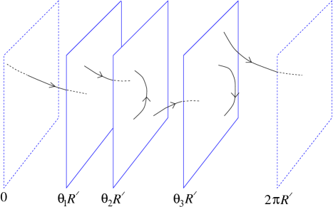
Figure 17: Three D–branes at different positions, with various strings attached.

3.8 D–Brane Dynamics: Collective Coörds and Gauge Theory

Clearly, the whole picture goes through if several coordinates

$$X^{m}=\{X^{25},X^{24},\ldots,X^{p+1}\}$$ (171)

are periodic, and we rewrite the periodic dimensions in terms of the dual coordinates. The open string endpoints are then confined to $N$ $(p+1)$–dimensional hyperplanes, the D$(p+1)$–branes. The Neumann conditions on the world sheet, $\partial_{n}X^{m}(\sigma^{1},\sigma^{2})=0$, have become Dirichlet conditions $\partial_{t}X^{\prime m}(\sigma^{1},\sigma^{2})=0$ for the dual coordinates. In this terminology, the original 26 dimensional open string theory theory contains $N$ D25–branes. A 25–brane fills space, so the string endpoint can be anywhere: it just corresponds to an ordinary Chan–Paton factor.

It is natural to expect that the hyperplane is dynamical rather than rigid.[6] For one thing, this theory still has gravity, and it is difficult to see how a perfectly rigid object could exist. Rather, we would expect that the hyperplanes can fluctuate in shape and position as dynamical objects. We can see this by looking at the massless spectrum of the theory, interpreted in the dual coordinates.

Taking for illustration the case where a single coordinate is dualised, consider the mass spectrum. The $D-1$ dimensional mass is

$$M^{2} = (p^{25})^{2}+{1\over{\alpha^{\prime}}}({N}-1)$$ (172)

$$= \left({[2\pi n+(\theta_{i}-\theta_{j})]R^{\prime}\over 2\pi{\alpha^{\prime}}}\right)^{2}+{1\over{\alpha^{\prime}}}(N-1).$$

Note that $[2\pi n+(\theta_{i}-\theta_{j})]R^{\prime}$ is the minimum length of a string winding between hyperplanes $i$ and $j$. Massless states arise generically only for non–winding (i.e., $n=0$) open strings whose end points are on the same hyperplane, since the string tension contributes an energy to a stretched string. We have therefore the massless states (with their vertex operators):

$$\alpha^{\mu}_{-1}|{k};ii\rangle, V=\partial_{t}X^{\mu},$$

$$\alpha^{m}_{-1}|{k};ii\rangle, V=\partial_{t}X^{25}=\partial_{n}X^{\prime 25}.$$ (173)

The first of these is a gauge field living on the D–brane, with $p+1$ components tangent to the hyperplane, $A^{\mu}(\xi^{a})$, $\mu,a=0,\ldots,p$. Here, $\xi^{\mu}=x^{\mu}$ are coordinates on the D–branes’ world–volume. The second was the gauge field in the compact direction in the original theory. In the dual theory it becomes the transverse position of the D–brane (see (170)). From the point of view of the world–volume, it is a family of scalar fields, $\Phi^{m}(\xi^{a})$, ($m=p+1,\ldots,D-1$) living there.

We saw this in equation (170) for a Wilson line, which was a constant gauge potential. Now imagine that, as genuine scalar fields, the $\Phi^{m}$ vary as we move around on the world–volume of the D–brane. This therefore embeds the brane into a variable place in the transverse coordinates. This is simply describing a specific shape to the brane as it is embedded in spacetime. The $\Phi^{m}(\xi^{a})$ are exactly analogous to the embedding coordinate map $X^{\mu}(\sigma,\tau)$ with which we described strings in the earlier sections.

The values of the gauge field backgrounds describe the shape of the branes as a soliton background, then. Meanwhile their quanta describe fluctuations of that background. This is the same phenomenon which we found for our description of spacetime in string theory. We started with strings in a flat background and discover that a massless closed string state corresponds to fluctuations of the geometry. Here we found first a flat hyperplane, and then discovered that a certain open string state corresponds to fluctuations of its shape. Remarkably, these open string states are simply gauge fields, and this is one of the reasons for the great success of D–branes. There are other branes in string theory (as we shall see) and they have other types of field theory describing their collective dynamics. D–branes are special, in that they have a beautiful description using gauge theory. Ultimately, we can use the long experience of working with gauge theories to teach us much about D–branes, and later, the geometry of D–branes and the string theories in which they live can teach us a lot about gauge theories. This is the basis of the dialogue between gauge theory and geometry which dominates the field at present.

It is interesting to look at the $U(N)$ symmetry breaking in the dual picture where the brane can move transverse to their world–volumes. When no D–branes coincide, there is just one massless vector each, or $U(1)^{N}$ in all, the generic unbroken group. If $k$ D–branes coincide, there are new massless states because strings which are stretched between these branes can achieve vanishing length. Thus, there are $k^{2}$ vectors, forming the adjoint of a $U(k)$ gauge group.[23, 24] This coincident position corresponds to $\theta_{1}=\theta_{2}=\cdots=\theta_{k}$ for some subset of the original $\{\theta\}$, so in the original theory the Wilson line left a $U(k)$ subgroup unbroken. At the same time, there appears a set of $k^{2}$ massless scalars: the $k$ positions are promoted to a matrix. This is curious and hard to visualise, but plays an important role in the dynamics of D–branes.[24] We will examine many consequences of this later in these notes. Note that if all $N$ branes are coincident, we recover the $U(N)$ gauge symmetry.

While this picture seems a bit exotic, and will become more so in the unoriented theory, the reader should note that all we have done is to rewrite the original open string theory in terms of variables which are more natural in the limit $R\ll\sqrt{{\alpha^{\prime}}}$. Various puzzling features of the small–radius limit become clear in the T–dual picture.

Observe that, since T–duality interchanges Neumann and Dirichlet boundary conditions, a further T–duality in a direction tangent to a D$p$–brane reduces it to a D$(p-1)$–brane, while a T–duality in a direction orthogonal turns it into a D$(p+1)$–brane.

3.9 T–Duality and Orientifolds.

The $R\to 0$ limit of an unoriented theory also leads to a new extended object. Recall that the effect of T–duality can also be understood as a one–sided parity transformation. For closed strings, the original coordinate is $X^{m}(z,\bar{z})=X^{m}(z)+X^{m}(\bar{z})$. We have already discussed how to project string theory with these coordinates by $\Omega$. The dual coordinate is $X^{\prime m}(z,\bar{z})=X^{m}(z)-X^{m}(\bar{z})$. The action of world sheet parity reversal is to exchange $X^{\mu}(z)$ and $X^{\mu}(\bar{z})$. This gives for the dual coordinate:

$$X^{\prime m}(z,\bar{z})\leftrightarrow-X^{\prime m}(\bar{z},z)\ .$$ (174)

This is the product of a world–sheet and a spacetime parity operation. In the unoriented theory, strings are invariant under the action of $\Omega$, while in the dual coordinate the theory is invariant under the product of world–sheet parity and a spacetime parity. This generalisation of the usual unoriented theory is known as an “orientifold”, a term which mixes the term “orbifold” with orientation reversal.

Imagine that we have separated the string wavefunction into its internal part and its dependence on the centre of mass, $x^{m}$. Furthermore, take the internal wavefunction to be an eigenstate of $\Omega$. The projection then determines the string wavefunction at $-x^{m}$ to be the same as at $x^{m}$, up to a sign. In practice, the various components of the metric and antisymmetric tensor satisfy e.g.,

$$G_{\mu\nu}(x^{\mu},-x^{m})=G_{\mu\nu}(x^{\mu},x^{m}), B_{\mu\nu}(x^{\mu},-x^{m})=-B_{\mu\nu}(x^{\mu},x^{m}),$$

$$G_{\mu n}(x^{\mu},-x^{m})=-G_{\mu n}(x^{\mu},x^{m}), B_{\mu n}(x^{\mu},-x^{m})=B_{\mu n}(x^{\mu},x^{m}),$$

$$G_{mn}(x^{\mu},-x^{m})=G_{mn}(x^{\mu},x^{m}), B_{mn}(x^{\mu},-x^{m})=-B_{mn}(x^{\mu},x^{m})\ .$$ (175)

In other words, when we have $k$ compact directions, the T–dual spacetime is the torus $T^{25-k}$ modded by a ${\hbox{{\rm Z}\kern-3.99994pt\hbox{\rm Z}}}_{2}$ reflection in the compact directions. So we are instructed to perform an orbifold construction, modified by the extra sign. In the case of a single periodic dimension, for example, the dual spacetime is the line segment $0\leq x^{25}\leq\pi R^{\prime}$. The reader should remind themselves of the orbifold construction in section 3.6. At the ends of the interval, there are fixed “points” , which are in fact spatially 24–dimensional planes. Looking at the projections (175) in this case, we see that on these fixed planes, the projection is just like we did for the $\Omega$–projection of the 25+1 dimensional theory in section 2.6: The theory is unoriented there, and half the states are removed. These orientifold fixed planes are called “O–planes” for short. For this case, we have two O24–planes. (For $k$ directions we have $2^{k}$ O$(25-k)$–planes arranged on the vertices of a hypercube.) In particular, we can usefully think of the original case of $k=0$ as being on an O25–plane.

While the theory is unoriented on the O–plane, away from the orientifold fixed planes, the local physics is that of the oriented string theory. The projection relates the physics of a string at some point $x^{m}$ to the string at the image point $-x^{m}$.

In string perturbation theory, orientifold planes are not dynamical. Unlike the case of D–branes, there are no string modes tied to the orientifold plane to represent fluctuations in its shape. Our heuristic argument in the previous subsection that gravitational fluctuations force a D–brane to move dynamically does not apply to the orientifold fixed plane. This is because the identifications (175) become boundary conditions at the fixed plane, such that the incident and reflected gravitational waves cancel. For the D–brane, the reflected wave is higher order in the string coupling.

The orientifold construction was discovered via T–duality [6] and independently from other points of view.[25, 8] One can of course consider more general orientifolds which are not simply T–duals of toroidal compactifications. The idea is simply to combine a group of discrete symmetries with $\Omega$ such that the resulting group of operations (the “orientifold group”, $G_{\Omega}$) is itself a symmetry of some string theory. One then has the right to ask what the nature of the projected theory obtained by dividing by $G_{\Omega}$ might be. This is a fruitful way of construction interesting and useful string vacua. [26] We shall have more to say about this later, since in superstring theory we shall find that O–planes, like D–branes , are sources of various closed string sector fields. Therefore there will be additional consistency conditions to be satisfied in constructing an orientifold, amounting to making sure that the field equations are satisfied.

So far our discussion of orientifolds was just for the closed string sector. Let us see how things are changed in the presence of open strings. In fact, the situation is similar. Again, let us focus for simplicity on a single compact dimension. Again there is one orientifold fixed plane at $0$ and another at $\pi R^{\prime}$. Introducing $SO(N)$ Chan–Paton factors, a Wilson line can be brought to the form

$${\rm diag}\{\theta_{1},-\theta_{1},\theta_{2},-\theta_{2},\cdots,\theta_{N/2},-\theta_{N/2}\}.$$ (176)

Thus in the dual picture there are ${1\over 2}N$ D–branes on the line segment $0\leq X^{\prime 25}<\pi R^{\prime}$, and ${1\over 2}N$ at their image points under the orientifold identification.

Strings can stretch between D–branes and their images as shown in figure 18.

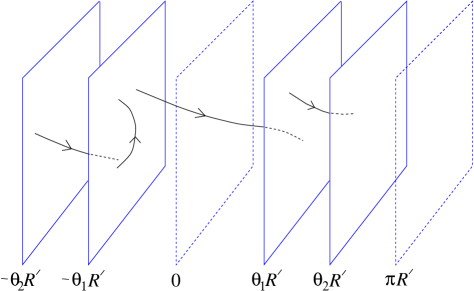
Figure 18: Orientifold planes at $0$ and $\pi R^{\prime}$. There are D–branes at $\theta_{1}R^{\prime}$ and $\theta_{2}R^{\prime}$, and their images at -$\theta_{1}R^{\prime}$ and $-\theta_{2}R^{\prime}$. $\Omega$ acts on any string by a combination of a spacetime reflection through the planes and reversing the orientation arrow.

The generic gauge group is $U(1)^{N/2}$, where all branes are separated. As in the oriented case, if $m$ D–branes are coincident there is a $U(m)$ gauge group. However, now if the $m$ D–branes in addition lie at one of the fixed planes, then strings stretching between one of these branes and one of the image branes also become massless and we have the right spectrum of additional states to fill out $SO(2m)$. The maximal $SO(N)$ is restored if all of the branes are coincident at a single orientifold plane. Note that this maximally symmetric case is asymmetric between the two fixed planes. Similar considerations apply to $USp(N)$. As we saw before, the difference between the appearance of the two groups is in a sign on the matrix $M$ as it acts on the string wavefunction. Later, we shall see that this sign is correlated with the sign of the charge and tension of the orientifold plane.

We should emphasise that there are $\frac{1}{2}N$ dynamical D–branes but an $N$–valued Chan–Paton index. An interesting case is when $k+\frac{1}{2}$ D–branes lie on a fixed plane, which makes sense because the number $2k+1$ of indices is integer. A brane plus image can move away from the fixed plane, but the number of branes remaining is always half–integer. This anticipates a discussion which we shall have about fractional branes much later, in section 9.2 even outside the context of orientifolds.

3.10 The D–Brane Tension

The D–brane is a dynamical object, and as such, feels the force of gravity. The tension of the brane controls its response to outside influences which try to make it change its shape, absorb energy, etc., just as we saw for the tension of a string. If we introduce coordinates $\xi^{a}$, $a=0,\ldots p$ on the brane, we can begin to write an action for the dynamics of the brane in terms of fields living on the world–volume in much the same way that we did for the string, in terms of fields living on the world–sheet. As we discussed before, the fields on the brane are the embedding $X^{\mu}(\xi)$ and the gauge field $A_{a}(\xi)$. We shall ignore the latter for now and concentrate just on the embedding part, which is enough to get the tension right. The action is (again by direct analogy to the particle and string case)

$$S_{p}=-T_{p}\int d^{p+1}\xi\,e^{-\Phi}\det\!^{1/2}G_{ab}\ ,$$ (177)

where $G_{ab}$ is the induced metric on the brane, otherwise known as the “pull–back” of the spacetime metric $G_{\mu\nu}$ to the brane:

$$G_{ab}\equiv{\partial X^{\mu}\over\partial\xi^{a}}{\partial X^{\nu}\over\partial\xi^{b}}G_{\mu\nu}\ .$$ (178)

$T_{p}$ is the tension of the D$p$–brane. The dilaton dependence $e^{-\Phi}=g_{s}^{-1}$ arises because this is an open string tree level action.

Before computing the tension, we should note that we can get a recursion relation for it from T–duality[59, 27] The mass of a D$p$–brane wrapped around a $p$–torus $T^{p}$ is

$$T_{p}e^{-\Phi}\prod_{i=1}^{p}(2\pi R_{i})\ .$$ (179)

T–dualising on the single direction $X^{p}$ and recalling the transformation (139) of the dilaton, we can rewrite the mass (179) in the dual variables:

$$T_{p}(2\pi\sqrt{{{\alpha^{\prime}}}})e^{-\Phi^{\prime}}\prod_{i=1}^{p-1}(2\pi R_{i})\ =\ T_{p-1}e^{-\Phi^{\prime}}\prod_{i=1}^{p-1}(2\pi R_{i})\ .$$ (180)

Hence,

$$T_{p}=T_{p-1}/2\pi\sqrt{{{\alpha^{\prime}}}}\qquad\Rightarrow\qquad T_{p}=T_{p^{\prime}}(2\pi\sqrt{\alpha^{\prime}})^{p^{\prime}-p}\ .$$ (181)

Where we performed the duality recursively to deduce the general relation.

Let us now compute the D–brane tension $T_{p}$. As noted above, it is proportional to $g_{s}^{-1}$. One could calculate it from the gravitational coupling to the D–brane, given by the disk with a graviton vertex operator. However, it is much easier to obtain the absolute normalisation as follows. Consider two parallel D$p$–branes at positions $X^{\prime\mu}=0$ and $X^{\prime\mu}=Y^{\mu}$. These two objects can feel each other‘s presence by exchanging closed strings as shown in figure 19.

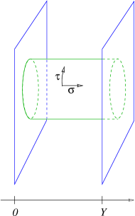
Figure 19: Exchange of a closed string between two D–branes. This is equivalent to a vacuum loop of an open string with one end on each D–brane.

This string graph is an annulus, with no vertex operators. It is therefore as easily calculated as our closed string one loop amplitudes done earlier. Extracting the poles from graviton and dilaton exchange then give the coupling $T_{p}$ of closed string states to the D–brane.

Let us parametrise the string world–sheet as $(\sigma^{2}=\tau,\sigma^{1}=\sigma)$ where now $\tau$ is periodic and runs from $0$ to $2\pi t$, and $\sigma$ runs (as usual) from $0$ to $\pi$. This vacuum graph (a cylinder) has the single modulus $t$, running from $0$ to $\infty$. If we slice horizontally, so that $\sigma^{2}=\tau$ is world–sheet time, we get an open string going in a loop. If we instead slice vertically, so that $\sigma$ is time, we see a single closed string propagating in the tree channel. (The world–line of the open string boundary can be regarded as a vertex connecting the vacuum to the single closed string, i.e., a one–point closed string vertex, [28, 29] which is a useful picture in the “boundary state” formalism, which we will not use here.)

This diagram will occur explicitly again in these lectures. It also appears implicitly in many other modern aspects in this series of lectures in this school and beyond: String theory produces many examples where one–loop gauge/field theory results (open strings) are related to tree level geometrical/gravity results. This is all organised by diagrams of this form, and is the basis of much of the gauge theory/geometry correspondences to be discussed.

Let us consider the limit $t\to 0$ of the loop amplitude. This is the ultra–violet limit for the open string channel, since the circle of the loop is small. However, this limit is correctly interpreted as an infrared limit of the closed string. (This is one of the earliest “dualities” of string theory, discussed even before it was known to be a theory of strings.) Time–slicing vertically shows that the $t\to 0$ limit is dominated by the lowest lying modes in the closed string spectrum. This all fits with the idea that there are no “ultraviolet limits” of the moduli space which could give rise to high energy divergences. They can always be related to amplitudes which have a handle pinching off. This physics is controlled by the lightest states, or the long distance physics. (This relationship is responsible for the various “UV/IR” relations which are a popular feature of current research.)

One–loop vacuum amplitudes are given by the Coleman–Weinberg formula, which can be thought of as the sum of the zero point energies of all the modes: (see insert 7 (p.3.10)) [32]

$${\cal A}=V_{p+1}\int\frac{d^{p+1}k}{(2\pi)^{p+1}}\int_{0}^{\infty}{dt\over 2t}\sum_{I}e^{-2\pi{\alpha^{\prime}}t(k^{2}+M_{I}^{2})}.$$ (182)

Here the sum $I$ is over the physical spectrum of the string, i.e., the transverse spectrum, and the momentum $k$ is in the $p+1$ extended directions of the D–brane world–sheet.

Insert 7: Vacuum Energy The Coleman–Weinberg formula evaluates the one–loop vacuum amplitude, which is simply the logarithm of the partition function ${\cal A}=Z_{\rm vac}$ for the complete theory: $$\ln\left(Z_{\rm vac}\right)=-{1\over 2}{\rm Tr}\ln\left(\Box^{2}+M^{2}\right)=-{V_{D}\over 2}\int{d^{D}k\over(2\pi)^{D}}\ln\left(k^{2}+M^{2}\right)\ .$$ But since we can write $$-{1\over 2}\ln(k^{2}+M^{2})=\int_{0}^{\infty}{dt\over 2t}e^{-{(k^{2}+M^{2})}t/2}\ ,$$ we have $${\cal A}=V_{D}\int{d^{D}k\over(2\pi)^{D}}\int_{0}^{\infty}{dt\over 2t}e^{-{(k^{2}+M^{2})}t/2}\ .$$ Recall finally that $(k^{2}+M^{2})/2$ is just the Hamiltonian, $H$, which in our case is just $L_{0}/\alpha^{\prime}$ (see (63)).

Insert 8: Translating Closed to Open Compare our open string appearance of $f_{1}(q)$, for $q=e^{-2\pi t}$ with the expressions for $f_{1}(q)$, ($q=e^{2\pi\tau}$) defined in our closed string discussion in (148). Here the argument is real. The translation between definitions is done by setting $t=-{\rm Im}\,\tau$. From the modular transformations (150), we can deduce some useful asymptotia. While the asymptotics as $t\to\infty$ are obvious, we can get the $t\to 0$ asymptotics using (150) $$f_{1}(e^{-{\pi}/{s}})=\sqrt{s}\,f_{1}(e^{-\pi s}),\quad f_{3}(e^{-{\pi}/{s}})=f_{3}(e^{-\pi s}),\quad f_{2}(e^{-{\pi}/{s}})=f_{4}(e^{-\pi s}).$$ (183)

The mass spectrum is given by

$$M^{2}={1\over{\alpha^{\prime}}}\left(\sum_{n=1}^{\infty}{\alpha}^{i}_{-n}\alpha_{n}^{i}-1\right)+{Y\cdot Y\over 4\pi^{2}\alpha^{\prime 2}}$$ (184)

where $Y^{m}$ is the separation of the D–branes. The sums over the oscillator modes work just like the computations we did before (see insert 4 (p.2.5)), giving

$${\cal A}=2V_{p+1}\int_{0}^{\infty}{dt\over 2t}(8\pi^{2}{\alpha^{\prime}}t)^{-{(p+1)\over 2}}e^{-Y\cdot Yt/2\pi{\alpha^{\prime}}}f_{1}(q)^{-24}\ .$$ (185)

Here $q=e^{-2\pi t}$, and the overall factor of 2 is from exchanging the two ends of the string. (See insert 8 (p.3.10) for news of $f_{1}(q)$)

In the present case, (using the asymptotics derived in insert 8)

$${\cal A}=2V_{p+1}\int_{0}^{\infty}{dt\over 2t}(8\pi^{2}{\alpha^{\prime}}t)^{-{(p+1)\over 2}}e^{-Y\cdot Yt/2\pi{\alpha^{\prime}}}t^{12}\left(e^{2\pi/t}+24+\ldots\right).$$ (186)

The leading divergence is from the tachyon and is an uninteresting bosonic artifact. The massless pole, from the second term, is

$${\cal A} \sim V_{p+1}{24\over 2^{12}}(4\pi^{2}{\alpha^{\prime}})^{11-p}\pi^{(p-23)/2}\Gamma((23-p)/2)|Y|^{p-23}$$ (187)

$$= V_{p+1}{24\pi\over 2^{10}}(4\pi^{2}{\alpha^{\prime}})^{11-p}G_{25-p}(Y^{2})$$

where $G_{d}(Y^{2})$ is the massless scalar Green’s function in $d$ dimensions.

We can compare this with a field theory calculation, the exchange of graviton plus dilaton between a pair of D–branes. The propagator is from the bulk action (111) and the couplings are from the D–brane action (177). This is a bit of effort because the graviton and dilaton mix, but in the end one finds

$${\cal A}\sim{D-2\over 4}V_{p+1}T_{p}^{2}\kappa_{0}^{2}G_{25-p}(Y^{2})$$ (188)

and so

$$T_{p}={\sqrt{\pi}\over 16\kappa_{0}}(4\pi^{2}{\alpha^{\prime}})^{(11-p)/2}\ .$$ (189)

This agrees with the recursion relation (181). The actual D–brane tension includes a factor of the string coupling from the action (177),

$$\tau_{p}={\sqrt{\pi}\over 16\kappa}(4\pi^{2}{\alpha^{\prime}})^{(11-p)/2}\$$ (190)

where $\kappa=\kappa_{0}g_{s}$, and we shall use $\tau$ this to denote the tension when we include the string coupling henceforth, and reserve $T$ for situations where the string coupling is included in the background field $e^{-\Phi}$.( This will be less confusing than it sounds, since it will always be clear from the context which we mean.)

Notice then that the tension $\tau_{p}$ of a D$p$–brane is of order $g_{s}^{-1}$. This follows from the fact that the diagram connecting the brane to the closed string sector is a disc diagram, and insert 5 (p.2.6) shows reminds us that this is of order $g_{s}^{-1}$. An immediate consequence of this is that they will produce non–perturbative effects of order $\exp(-1/g_{s})$ in string theory, since their action is of the same order as their mass.

Formula (189) will not concern us much beyond these sections, since we will derive a new one for the superstring case later.

The asymptotics (186) can be interpreted in terms of a sum over closed string states exchanged between the two D–branes. One can write the cylinder path integral in Hilbert space formalism treating $\sigma_{1}$ rather than $\sigma_{2}$ as time. It then has the form

$$\langle B|e^{-(L_{0}+\tilde{L}_{0})\pi/t}|B\rangle$$ (191)

where the boundary state $|B\rangle$ is the closed string state created by the boundary loop. We will not have time to develop this formalism but it is useful in finding the couplings between closed and open strings.[28, 29]

3.11 The Orientifold Tension

The O–plane, like the D–brane, couples to the dilaton and metric. The amplitude is the same as in the previous section, but with $\mathbf{RP}^{2}$ in place of the disk; i.e., a crosscap replaces the boundary loop. The orientifold identifies $X^{m}$ with $-X^{m}$ at the opposite point on the crosscap, so the crosscap is localised near one of the orientifold fixed planes. Again the easiest way to calculate this is via vacuum graphs, the cylinder with one or both boundary loops replaced by crosscaps. These give the Möbius strip and Klein bottle, respectively. To understand this, consider figure 20, which shows two copies of the fundamental region for the Möbius strip.

Figure 20: Two copies of the fundamental region for the Möbius strip.

The lower half is identified with the reflection of the upper, and the edges $\sigma^{1}=0,\pi$ are boundaries. Taking the lower half as the fundamental region gives the familiar representation of the Möbius strip as a strip of length $2\pi t$, with ends twisted and glued. Taking instead the left half of the figure, the line $\sigma^{1}=0$ is a boundary loop while the line $\sigma^{1}=\pi/2$ is identified with itself under a shift $\sigma^{2}\to\sigma^{2}+2\pi t$ plus reflection of $\sigma^{1}$: it is a crosscap. The same construction applies to the Klein bottle, with the right and left edges now identified. Another way to think of the Möbius strip amplitude we are going to compute here is as representing the exchange of a closed string between a D—brane and its mirror image, as shown in figure 21. The identification with a twist is performed on the two D–branes, turning the cylinder into a Möbius strip.

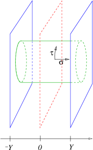
Figure 21: The Möbius strip as the exchange of closed strings between a brane and its mirror image. The dotted plane is the orientifold plane.

The Möbius strip is given by the vacuum amplitude

$${\cal A}_{\rm M}=V_{p+1}\int\frac{d^{p+1}k}{(2\pi)^{p+1}}\int_{0}^{\infty}{dt\over 2t}\sum_{I}{\Omega_{i}\over 2}e^{-2\pi{\alpha^{\prime}}t(p^{2}+M_{I}^{2})},$$ (192)

where $\Omega_{I}$ is the $\Omega$ eigenvalue of state $i$. The oscillator contribution to $\Omega_{I}$ is $(-1)^{N}$ from eq. (99).  For the $SO(N)$ open string the Chan–Paton factors have ${1\over 2}N(N+1)$ even states and ${1\over 2}N(N-1)$ odd for a net of $+N$. For $USp(N)$ these numbers are reversed for a net of $-N$. Focus on a D–brane and its image, which correspondingly contribute $\pm 2$. The diagonal elements, which contribute to the trace, are those where one end is on the D–brane and one on its image. The total separation is then $Y^{m}=2X^{m}$. Then,

$${\cal A}_{\rm M} = \pm V_{p+1}\int_{0}^{\infty}{dt\over 2t}(8\pi^{2}{\alpha^{\prime}}t)^{-{(p+1)\over 2}}e^{-2X\cdot Xt/\pi{\alpha^{\prime}}}\times$$ (193)

$$\qquad\qquad\qquad\qquad\qquad\times\left[q^{-2}\prod_{k=1}^{\infty}(1+q^{4k-2})^{-24}(1-q^{4k})^{-24}\right]$$

The factor in braces is

$$f_{3}(q^{2})^{-24}f_{1}(q^{2})^{-24} = (2t)^{12}f_{3}(e^{-\pi/2t})^{-24}f_{1}(e^{-\pi/2t})^{-24}$$ (194)

$$= (2t)^{12}\left(e^{\pi/2t}-24+\ldots\right)\ .$$

One thus finds a pole

$$\mp 2^{p-12}V_{p+1}{3\pi\over 2^{6}}(4\pi^{2}{\alpha^{\prime}})^{11-p}G_{25-p}(X^{2})\ .$$ (195)

This is to be compared with the field theory result ${D-2\over 2}V_{p+1}T_{p}T^{\prime}_{p}\kappa_{0}^{2}G_{25-p}(Y^{2})$, where $T^{\prime}_{p}$ is the O–plane tension. A factor of 2 as compared to the earlier field theory calculation (188) comes because the spacetime boundary forces all the flux in one direction. Thus the O–plane and D–brane tensions are related

$$\tau^{\prime}_{p}=\mp 2^{p-13}\tau_{p}.$$ (196)

A similar calculation with the Klein bottle gives a result proportional to $\tau_{p}^{\prime 2}$.

Noting that there are $2^{25-p}$ O–planes, the total O–plane source is $\mp 2^{12}\tau_{p}$. The total source must vanish because the volume is finite and there is no place for flux to go. Thus there are $2^{(D-2)/2}=2^{12}$ D–branes (times two for the images) and the group is $SO(2^{13})=SO(2^{D/2})$.[33] For this group the “tadpoles” associated with the dilaton and graviton, representing violations of the field equations, cancel at order $g_{s}^{-1}$. This has no special significance in the bosonic string, as the one loop $g_{s}^{0}$ tadpoles are nonzero and imaginary due to the tachyon instability, but similar considerations will give a restriction on anomaly free Chan–Paton gauge groups in the superstring.

4 Worldvolume Actions I: Dirac–Born–Infeld

In the previous section, we wrote only part of the world–volume action for the D–branes: that involving the embedding fields $X^{m}(\xi)=2\pi\alpha^{\prime}\Phi^{m}(\xi)$ ($m=p+1,\ldots,D-1$) and their coupling given by the induced metric on the worldvolume. We should expect, however, to have to take into account new couplings for the $X^{m}(\xi)$ as a result of other background spacetime fields like the antisymmetric tensor $B_{\mu\nu}$, which must again appear as an induced tensor $B_{ab}$ on the worldvolume, via a formula like (178). (Recall that $a=0,\ldots,p$). Furthermore, we should also write the action for the collective modes which we uncovered in section 3.8, the world–volume gauge fields $A^{a}(\xi)$.

The first thing to notice that that there is a restriction due to spacetime gauge symmetry on the precise combination of $B_{ab}$ and $A^{a}$ which can appear in the action. The combination $B_{ab}+2\pi{\alpha^{\prime}}F_{ab}$ can be understood as follows. In the world–sheet sigma model action of the string, we have the usual closed string term (108) for $B$ and the boundary action (113) for $A$. So the fields appear in the combination:

$${1\over 2\pi\alpha^{\prime}}\int_{\cal M}B+\int_{\partial\cal M}A\ .$$ (197)

We have written everything in terms of differential forms, since $B$ and $A$ are antisymmetric. For example $\int A\equiv\int A_{a}d\xi^{a}$.

This action is invariant under the spacetime gauge transformation $\delta A=d\lambda$. However, the spacetime gauge transformation $\delta B=d\zeta$ will give a surface term which must be cancelled with the following gauge transformation of $A$: $\delta A=-\zeta/2\pi\alpha^{\prime}$. So the combination $B+2\pi\alpha^{\prime}F$, where $F=dA$ is invariant under both symmetries; This is the combination of $A$ and $B$ which must appear in the action in order for spacetime gauge invariance to be preserved.

4.1 Tilted D–Branes

There are many ways to deduce the world–volume action. One way is to simply redo the computation for Weyl invariance of the complete sigma model, including the boundary terms, which will result in the $p+1$–dimensional equations of motion for the worldvolume fields $G_{ab}$ $B_{ab}$ and $A_{a}$. One can then deduce the $p+1$–dimensional worldvolume action from which those equations of motion may be derived. We will comment on this below.

Another way is to use T–duality to build the action piece by piece. For the purposes of these lectures and the various applications, this second way is perhaps more instructive.

Consider[34, 35, 36] a D2–brane extended in the $X^{1}$ and $X^{2}$ directions, and let there be a constant gauge field $F_{12}$. (We leave the other dimensions unspecified, so the brane could be larger by having extent in other directions. This will not affect our discussion.) We can choose a gauge in which $A_{2}=X^{1}F_{12}$. Now consider T–dualising along the 2-direction. The relation (170) between the potential and coordinate gives

$$X^{\prime 2}=2\pi{\alpha^{\prime}}X^{1}F_{12}\ ,$$ (198)

This says that the resulting D1–brane is tilted at an angle $\theta=\tan^{-1}(2\pi\alpha^{\prime}F_{12})$ to the $X^{2}$–axis! This gives a geometric factor in the D1–brane world–volume action,

$$S\sim\int_{\rm D1}ds=\int dX^{1}\,\sqrt{1+(\partial_{1}X^{\prime 2})^{2}}=\int dX^{1}\,\sqrt{1+(2\pi{\alpha^{\prime}}F_{12})^{2}}\ .$$ (199)

We can always boost the D–brane to be aligned with the coordinate axes and then rotate to bring $F_{\mu\nu}$ to block-diagonal form, and in this way we can reduce the problem to a product of factors like (199) giving a determinant:

$$S\sim\int d^{D}X\,\det\!^{1/2}(\eta_{\mu\nu}+2\pi\alpha^{\prime}F_{\mu\nu})\ .$$ (200)

This is the Born–Infeld action[37].

In fact, this is the complete action (in a particular “static” gauge which we will discuss later) for a space–filling D25–brane in flat space, and with the dilaton and antisymmetric tensor field set to zero. In the language of section 2.7, Weyl invariance of the open string sigma model (113) amounts to the following open string analogue of (110) for the open string sector:

$$\beta^{A}_{\mu}=\alpha^{\prime}\left({1\over 1-(2\pi\alpha^{\prime}F)^{2}}\right)^{\nu\lambda}\partial_{(\nu}F_{\lambda)\mu}=0\ ,$$ (201)

these equations of motion follow from the action. In fact, in contrast to the Maxwell action written previously (112), and the closed string action (111), this action is true to all orders in $\alpha^{\prime}$, although only for slowly varying field strengths; there are corrections from derivatives of $F_{\mu\nu}$. [30]

4.2 The Dirac–Born–Infeld Action

We can uncover a lot of the rest of the action by simply dimensionally reducing. Starting with (200), where $F_{\mu\nu}=\partial_{\mu}A_{\nu}-\partial_{\nu}A_{\mu}$ as usual (we will treat the non–Abelian case later) let us assume that $D-p-1$ spatial coordinates are very small circles, small enough that we can neglect all derivatives with respect to those directions, labelled $X^{m}$, $m=p+1,\ldots,D-1$. (The uncompactified coordinates will be labelled $X^{a}$, $a=0,\ldots,p$.) In this case, the matrix whose determinant appears in (200) is:

$$\pmatrix{N&-A^{T}\cr A&M}\ ,$$ (202)

where

$$N=\eta_{ab}+2\pi\alpha^{\prime}F_{ab}\ ;\qquad M=\delta_{mn}\ ;\qquad A=2\pi\alpha^{\prime}\partial_{a}A_{m}\ .$$ (203)

Using the fact that its determinant can be written as $|M||N+A^{T}M^{-1}A|$, our action becomes [46]

$$S\sim-\int d^{p+1}X\,\det\!^{1/2}(\eta_{ab}+\partial_{a}X^{m}\partial_{b}X_{m}+2\pi\alpha^{\prime}F_{ab})\ ,$$ (204)

up to a numerical factor (coming from the volume of the torus we reduced on. Once again, we used the T–duality rules (170) to replace the gauge fields in the T–dual directions by coordinates: $2\pi\alpha^{\prime}A_{m}=X^{m}$.

This is (nearly) the action for a D$p$–brane and we have uncovered how to write the action for the collective coordinates $X^{m}$ representing the fluctuations of the brane transverse to the world–volume. There now remains only the issue of putting in the case of non–trivial metric, $B_{\mu\nu}$ and dilaton. This is easy to guess given that which we have encountered already:

$$S_{p}=-T_{p}\int d^{p+1}\xi\,e^{-\Phi}\det\!^{1/2}(G_{ab}+B_{ab}+2\pi\alpha^{\prime}F_{ab})\ .$$ (205)

This is the Dirac–Born–Infeld Lagrangian, for arbitrary background fields. The factor of the dilaton is again a result of the fact that all of this physics arises at open string tree level, hence the factor $g_{s}^{-1}$, and the $B_{ab}$ is in the right place because of spacetime gauge invariance. $T_{p}$ and $G_{ab}$ are in the right place to match onto the discussion we had when we computed the tension. Instead of using T–duality, we could have also deduced this action by a generalisation of the sigma model methods described earlier, and in fact this is how it was first derived in this context. [31]

We have re–introduced independent coordinates $\xi^{a}$ on the world–volume. Note that the actions (199),(204) were written using a choice where we aligned the world–volume with the first $p+1$ spacetime coordinates as $\xi^{a}=X^{a}$, leaving the $D-p-1$ transverse coordinates called $X^{m}$. We can always do this using worldvolume and spacetime diffeomorphism invariance. This choice is called the “static gauge”, and we shall use it quite a bit in these notes. Writing this out (for vanishing dilaton) using the formula (178) for the induced metric, for the case of $G_{\mu\nu}=\eta_{\mu\nu}$ we see that we get the action (204).

4.3 The Action of T–Duality

It is amusing [36, 44] to note that our full action obeys (as it should) the rules of T–duality which we already wrote down for our background fields. The action for the D$p$–brane is built out of the determinant $|E_{ab}+2\pi\alpha^{\prime}F_{ab}|$, where the $(a,b=0,\ldots p)$ indices on $E_{ab}$ mean that we have performed the pullback of $E_{\mu\nu}$ (defined in (141)) to the worldvolume. This matrix becomes, if we T–dualise on $n$ directions labelled by $X^{i}$ and use the rules we wrote in (142):

$$\left|\matrix{E_{ab}-E_{ai}E^{ij}E_{jb}+2\pi\alpha^{\prime}F_{ab}&-E_{ak}E^{kj}-2\pi\alpha^{\prime}\partial_{a}X^{i}\cr E^{ik}E_{kb}+2\pi\alpha^{\prime}\partial_{b}X^{i}&E^{ij}}\right|\ ,$$ (206)

which has determinant $|E^{ij}||E_{ab}+2\pi\alpha^{\prime}F_{ab}|$. In forming the square root, we get again the determinant needed for the definition of a T–dual DBI action, as the extra determinant $|E^{ij}|$ precisely cancels the determinant factor picked up by the dilaton under T–duality. (Recall, $E^{ij}$ is the inverse of $E_{ij}$.)

Furthermore, the tension $T_{p^{\prime}}$ comes out correctly, because there is a factor of $\Pi_{i}^{n}(2\pi R_{i})$ from integrating over the torus directions, and a factor $\Pi_{i}^{n}(R_{i}/\sqrt{\alpha^{\prime}})$ from converting the factor $e^{-\Phi}$, (see (139)), which fits nicely with the recursion formula (181) relating $T_{p}$ and $T_{p^{\prime}}$.

The above was done as though the directions on which we dualised were all Neumann or all Dirichlet. Clearly, we can also extrapolate to the more general case.

4.4 Non–Abelian Extensions

For $N$ D–branes the story is more complicated. The various fields on the brane representing the collective motions, $A_{a}$ and $X^{m}$, become matrices valued in the adjoint. In the Abelian case, the various spacetime background fields (here denoted $F_{\mu}$ for the sake of argument) which can appear on the worldvolume typically depend on the transverse coordinates $X^{m}$ in some (possibly) non–trivial way. In the non–Abelian case, with $N$ D–branes, the transverse coordinates are really $N\times N$ matrices, $2\pi\alpha^{\prime}\Phi^{m}$, since they are T–dual to non–Abelian gauge fields as we learned in previous sections, and so inherit the behaviour of gauge fields (see eqn.(170)). We write them as $\Phi^{m}=X^{m}/(2\pi\alpha^{\prime})$. So not only should the background fields $F_{\mu}$ depend on the Abelian part, but they ought to possibly depend (implicitly or explicitly) on the full non–Abelian part as $F(\Phi)_{\mu}$ in the action.

Furthermore, in (205) we have used the partial derivatives $\partial_{a}X^{\mu}$ to pull back spacetime indices $\mu$ to the worldvolume indices, $a$, e.g., $F_{a}=F_{\mu}\partial_{a}X^{\mu}$, and so on. To make this gauge covariant in the non–Abelian case, we should pull back with the covariant derivative: $F_{a}=F_{\mu}{\cal D}_{a}X^{\mu}=F_{\mu}({\partial}_{a}X^{\mu}+[A_{a},X^{\mu}])$.

With the introduction of non–Abelian quantities in all of these places, we need to consider just how to perform a trace, in order to get a gauge invariant quantity to use for the action. Starting with the fully Neumann case (200), a first guess is that things generalise by performing a trace (in the fundamental of $U(N)$) of the square rooted expression. The meaning of the ${\rm Tr}$ needs to be stated, It is proposed that is means the “symmetric” trace, denoted “STr” which is to say that one symmetrises over gauge indices, consequently ignoring all commutators of the field strengths encountered while expanding the action. [38] (This suggestion is consistent with various studies of scattering amplitudes and also the BPS nature of various non–Abelian soliton solutions. There is still apparently some ambiguity in the definition which results in problems beyond fifth order in the field strength. [39, 40, 41, 42, 43])

Once we have this action, we can then again use T–duality to deduce the form for the lower dimensional, D$p$–brane actions. The point is that we can reproduce the steps of the previous analysis, but keeping commutator terms such as $[A_{a},\Phi^{m}]$ and $[\Phi^{m},\Phi^{n}]$. We will not reproduce those steps here, as they are similar in spirit to that which we have already done (for a complete discussion, please consult some of the literature. [38, 39, 43, 44]). The resulting action is:

$$S_{p} = -T_{p}\int d^{p+1}\xi\,e^{-\Phi}{\cal L}\ ,\quad\mbox{where}$$

$${\cal L} = {\rm STr}\left\{{\det\!^{1/2}[E_{ab}+E_{ai}(Q^{-1}-\delta)^{ij}E_{jb}+2\pi\alpha^{\prime}F_{ab}]\det\!^{1/2}[Q^{i}_{\phantom{i}j}]}\right\}\ ,$$ (207)

where $Q^{i}_{\phantom{i}j}=\delta^{i}_{\phantom{i}j}+i2\pi\alpha^{\prime}[\Phi^{i},\Phi^{k}]E_{kj}$, and we have raised indices with $E^{ij}$.

4.5 Yang–Mills Theory

In fact, we are now in a position to compute the constant $C$ in eqn.(112), by considering $N$ D25–branes, which is the same as an ordinary (fully Neumann) $N$-valued Chan–Paton factor. Expanding the D25–brane Lagrangian (200) to second order in the gauge field, we get

$$-{T_{25}\over 4}(2\pi{\alpha^{\prime}})^{2}e^{-\Phi}{\rm Tr}F_{\mu\nu}F^{\mu\nu},$$ (208)

with the trace in the fundamental representation of $U(N)$. This gives the precise numerical relation between the open and closed string couplings.[53]

Actually, with Dirichlet and Neumann directions, performing the same expansion, and in addition noting that

$$\det[Q^{i}_{\phantom{i}j}]=1-{(2\pi\alpha^{\prime})^{2}\over 4}[\Phi^{i},\Phi^{j}][\Phi^{i},\Phi^{j}]+\cdots\ ,$$ (209)

one can write the leading order action (207) as

$$S_{p}=-{T_{p}(2\pi\alpha^{\prime})^{2}\over 4}\int d^{p+1}\xi\,e^{-\Phi}{\rm Tr}\left[F_{ab}F^{ab}+2{\cal D}_{a}\Phi^{i}{\cal D}_{a}\Phi^{i}+[\Phi^{i},\Phi^{j}]^{2}\right]\biggr{\}}\ .$$ (210)

This is the dimensional reduction of the $D$–dimensional Yang–Mills term, displaying the non–trivial commutator for the adjoint scalars. This is an important term in many modern applications, as we shall see. Note that the $(p+1)$–dimensional Yang–Mills coupling for the theory on the branes is

$$g^{2}_{{\rm YM},p}=g_{s}T_{p}^{-1}(2\pi\alpha^{\prime})^{-2}\ .$$ (211)

This is worth noting. With the superstring value of $T_{p}$ which we will compute later, it is used in many applications to give the correct relation between gauge theory couplings and string quantities.

4.6 BIons, BPS Saturation and Fundamental Strings

We can of course treat the Dirac–Born–Infeld action as an interesting theory in its own right, and seek for interesting solutions of it. These solutions will have both a $(p+1)$–dimensional interpretation and a $D$–dimensional one. [46, 47, 48, 49, 50]

We shall not dwell on this in great detail, but include a brief discussion here to illustrate an important point, and refer to the literature for more complete discussions. More details will appear when we get to the supersymmetric case. One can derive an expression for the energy density contained in the fields on the world–volume: [50]

$${\cal E}^{2}=E^{a}E^{b}F_{ca}F_{cb}+E^{a}E^{b}G_{ab}+{\rm det}(G+2\pi\alpha^{\prime}F)\ ,$$ (212)

where here the matrix $F_{ab}$ contains only the magnetic components (i.e. no time derivatives) and $E^{a}$ are the electric components, subject to the Gauss Law constraint ${\vec{\nabla}}\cdot{\vec{E}}=0$. Also, as before

$$G_{ab}=\eta_{ab}+\partial_{a}X^{m}\partial_{b}X^{m}\ ,\qquad m=p+1,\ldots,D-1\ .$$ (213)

Let us consider the case where we have no magnetic components and only one of the transverse fields, say $X^{25}$, switched on. In this case, we have

$${\cal E}^{2}=(1\pm{\vec{E}}\cdot{\vec{\nabla}}X^{25})^{2}+({\vec{E}}\mp{\vec{\nabla}}X^{25})^{2}\ ,$$ (214)

and so we see that we have the Bogomol’nyi condition

$${\cal E}\geq|{\vec{E}}\cdot{\vec{\nabla}}X^{25}|+1\ .$$ (215)

This condition is saturated if ${\vec{E}}=\pm{\vec{\nabla}}X^{25}$. In such a case, we have

$$\nabla^{2}X^{25}=0\qquad\Rightarrow\qquad X^{25}={c_{p}\over r^{p-2}}\ ,$$ (216)

a harmonic solution, where $c_{p}$ is a constant to be determined. The total energy (beyond that of the brane itself) is, integrating over the world–volume:

$$E_{\rm tot} = \lim_{\epsilon\to\infty}T_{p}\int_{\epsilon}^{\infty}r^{p-1}drd\Omega_{p-1}({\vec{\nabla}}X^{25})^{2}=\lim_{\epsilon\to\infty}T_{p}{c_{p}^{2}(p-2)\Omega_{p-1}\over\epsilon^{p-2}}$$ (217)

$$= \lim_{\epsilon\to\infty}T_{p}c_{p}(p-2)\Omega_{p-1}X^{25}(\epsilon)\ ,$$

where $\Omega_{p-1}$ is the volume of the sphere $S^{p-1}$ surrounding our point charge source, and we have cut off the divergent integral by integrating down to $r=\epsilon$. (We will save the case of $p=1$ for later. [115, 50]) Now we can choose a value of the electric flux such that we get $(p-2)c_{p}\Omega_{p-1}T_{p}=(2\pi\alpha^{\prime})^{-1}$.   Putting this into our equation for the total energy, we see that the (divergent) energy of our configuration is:

$$E_{\rm tot}={1\over 2\pi\alpha^{\prime}}X^{25}(\epsilon)\ .$$ (218)

What does this mean? Well, recall that $X^{25}(\xi)$ gives the transverse position of the brane in the $X^{25}$ direction. So we see that the brane has grown a semi–infinite spike at $r=0$, and the base of this spike is our point charge. The interpretation of the divergent energy is simply the (infinite) length of the spike multiplied by a mass per unit length. But this mass per unit length is precisely the fundamental string tension $T=(2\pi\alpha^{\prime})^{-1}$! In other words, the spike solution is the fundamental string stretched perpendicular to the brane and ending on it, forming a point electric charge, known as a “BIon”. See figure 22$(a)$. In fact, a general BIon includes the non–linear corrections to this spike solution, which we have neglected here, having only written the linearised solution.

It is a worthwhile computation to show that if test source with the same charges is placed on the brane, there is no force of attraction or repulsion between it and the source just constructed, as would happen with pure Maxwell charges. This is because our sources have in addition to electric charge, some scalar ($X^{25}$) charge, which can also be attractive or repulsive. In fact, the scalar charges are such that the force due to electromagnetic charges is cancelled by the force of the scalar charge, another characteristic property of these solutions, which are said to be “Bogomol’nyi–Prasad–Sommerfield” (BPS)–saturated.[51, 52] We shall encounter solutions with this sort of behaviour a number of times in what is to follow.

Because of this property, the solution is easily generalised to include any number of BIons, at arbitrary positions, with positive and negative charges. The two choices of charge simply represents strings either leaving from, or arriving on the brane. See figure 22$(b)$.

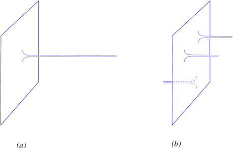
Figure 22: The $D$ dimensional interpretation of the BIon solution. $(a)$ It is an infinitely long spike representing a fundamental string ending on the D–brane. $(b)$ BIons are BPS and therefore can be added together at no cost to make a multi–BIon solution.

5 Superstrings and D–Branes

5.1 Open Superstrings: First Look

Let us go back to the beginning, almost. We can generalise the bosonic string action we had earlier to include fermions. In conformal gauge it is:

$$S={1\over 4\pi}\int_{\cal M}d^{2}\!\sigma\,\left\{{1\over\alpha^{\prime}}\partial X^{\mu}\bar{\partial}X_{\mu}+\psi^{\mu}\bar{\partial}\psi_{\mu}+\tilde{\psi}^{\mu}\partial\tilde{\psi}_{\mu}\right\}$$ (219)

where the open string world–sheet is the strip $0<\sigma<\pi$, $-\infty<\tau<\infty$.

N.B.: Actually, $\alpha^{\prime}$ is the loop expansion parameter analogous to $\hbar$ on worldsheet. It is therefore natural for the fermions’ kinetic terms to be normalised in this way.

We get a modification to the energy–momentum tensor from before (which we now denote as $T_{B}$, since it is the bosonic part):

$$T_{B}(z)=-{1\over\alpha^{\prime}}\partial X^{\mu}\partial X_{\mu}-{1\over 2}\psi^{\mu}\partial\psi_{\mu}\ ,$$ (220)

which is now accompanied by a fermionic energy–momentum tensor:

$$T_{F}(z)=i{2\over\alpha^{\prime}}\psi^{\mu}\partial X_{\mu}\ .$$ (221)

This enlarges our theory somewhat, while much of the logic of what we did in the purely bosonic story survives intact here. Now, one extremely important feature which we encountered in section 3.5 is the fact that the equations of motion admit two possible boundary conditions on the world–sheet fermions consistent with Lorentz invariance. These are denoted the “Ramond” (R) and the “Neveu–Schwarz” (NS) sectors:

$${\rm R\colon} \psi^{\mu}(0,\tau)=\tilde{\psi^{\mu}}(0,\tau)\qquad\psi^{\mu}(\pi,\tau)=\tilde{\psi^{\mu}}(\pi,\tau)$$

$${\rm NS\colon} \psi^{\mu}(0,\tau)=-\tilde{\psi^{\mu}}(0,\tau)\qquad\psi^{\mu}(\pi,\tau)=\tilde{\psi^{\mu}}(\pi,\tau)$$ (222)

We are free to choose the boundary condition at, for example the $\sigma=\pi$ end, in order to have a $+$ sign, by redefinition of $\tilde{\psi}$. The boundary conditions and equations of motion are summarised by the “doubling trick”: Take just left–moving (analytic) fields $\psi^{\mu}$ on the range $0$ to $2\pi$ and define $\tilde{\psi}^{\mu}(\sigma,\tau)$ to be $\psi^{\mu}(2\pi-\sigma,\tau)$. These left–moving fields are periodic in the Ramond (R) sector and antiperiodic in the Neveu-Schwarz (NS).

On the complex $z$–plane, the NS sector fermions are half–integer moded while the R sector ones are integer, and we have:

$$\psi^{\mu}(z)=\sum_{r}{\psi^{\mu}_{r}\over z^{r+1/2}}\ ,\,\,\mbox{where}\,\,{r\in{\hbox{{\rm Z}\kern-3.99994pt\hbox{\rm Z}}}}\,\mbox{or}\,\,{r\in{\hbox{{\rm Z}\kern-3.99994pt\hbox{\rm Z}}}+{\textstyle{1\over 2}}}$$ (223)

and canonical quantisation gives

$$\{\psi_{r}^{\mu},\psi^{\nu}_{s}\}=\{{\tilde{\psi}}_{r}^{\mu},{\tilde{\psi}}^{\nu}_{s}\}=\eta^{\mu\nu}\delta_{r+s}\ .$$ (224)

Similarly we have

$$T_{B}(z) = \sum_{m=-\infty}^{\infty}{L_{m}\over z^{m+2}}\quad\mbox{as before, and}$$

$$T_{F}(z) = \sum_{r}{G_{r}\over z^{r+3/2}}\ ,\,\,\mbox{where}\,\,{r\in{\hbox{{\rm Z}\kern-3.99994pt\hbox{\rm Z}}}}\,\,\mbox{(R)}\,\,\,\mbox{or}\,\,\,{{\hbox{{\rm Z}\kern-3.99994pt\hbox{\rm Z}}}+{\textstyle{1\over 2}}}\,\,\mbox{(NS)}$$ (225)

Correspondingly, the Virasoro algebra is enlarged, with the non–zero (anti) commutators being

$$[L_{m},L_{n}] = (m-n)L_{m+n}+{{\rm c}\over 12}(m^{3}-m)\delta_{m+n}$$

$$\{G_{r},G_{s}\} = 2L_{r+s}+{{\rm c}\over 12}(4r^{2}-1)\delta_{r+s}$$

$$\left[L_{m},G_{r}\right] = {1\over 2}(m-2r)G_{m+r}\ ,$$ (226)

with

$$L_{m} = {1\over 2}\sum_{m}:\alpha_{m-n}\cdot\alpha_{m}:+{1\over 4}\sum_{r}(2r-m):\psi_{m-r}\cdot\psi_{r}:+a\delta_{m,0}$$

$$G_{r} = \sum_{n}\alpha_{n}\cdot\psi_{r-n}\ .$$ (228)

In the above, $\rm c$ is the total contribution to the conformal anomaly, which is $D+D/2$, where $D$ is from the $D$ bosons while $D/2$ is from the $D$ fermions.

The values of $D$ and $a$ are again determined by any of the methods mentioned in the discussion of the bosonic string. For the superstring, it turns out that $D=10$ and $a=0$ for the R sector and $a=-1/2$ for the NS sector. This comes about because the contributions from the $X^{0}$ and $X^{1}$ directions are cancelled by the Faddev–Popov ghosts as before, and the contributions from the $\psi^{0}$ and $\psi^{1}$ oscillators are cancelled by the superghosts. Then, the computation uses the mnemonic/formula given in (79).

NS sector:zpe $$= 8\left(-{1\over 24}\right)+8\left(-{1\over 48}\right)=-{1\over 2}\ ,$$

R sector:zpe $$= 8\left(-{1\over 24}\right)+8\left({1\over 24}\right)=0\ .$$ (229)

As before, there is a physical state condition imposed by annihilating with the positive modes of the (super) Virasoro generators:

$$G_{r}|\phi\rangle=0\ ,\,\,\,r>0\ ;\quad L_{n}|\phi\rangle=0\ ,\,\,n>0\ ;\quad(L_{0}-a)|\phi\rangle=0\ .$$ (230)

The $L_{0}$ constraint leads to a mass formula:

$$M^{2}={1\over\alpha^{\prime}}\left(\sum_{n,r}\alpha_{-n}\cdot\alpha_{n}+r\psi_{-r}\cdot\psi_{r}-a\right)\ .$$ (231)

In the NS sector the ground state is a Lorentz singlet and is assigned odd fermion number, i.e., under the operator $(-1)^{F}$, it has eigenvalue $-1$.

In order to achieve spacetime supersymmetry, the spectrum is projected on to states with even fermion number. This is called the “GSO projection”,[54] and for our purposes, it is enough to simply state that this obtains spacetime supersymmetry, as we will show at the massless level. A more complete treatment —which gets it right for all mass levels— is contained in the full superconformal field theory. The GSO projection there is a statement about locality with the gravitino vertex operator.

Since the open string tachyon clearly has $(-1)^{F}=-1$, it is removed from the spectrum by GSO. This is our first achievement, and justifies our earlier practice of ignoring the tachyons appearance in the bosonic spectrum in what has gone before. Fro what we will do for the rest of the these notes, the tachyon will largely remain in the wings, but it (and other tachyons) do have a role to play, since they are often a signal that the vacuum wants to move to a (perhaps) more interesting place. We will see this in a couple of places before the end. (See John Schwarz’s discussion of the construction of non–BPS D–branes, in this school. [18])

Massless particle states in ten dimensions are classified by their $SO(8)$ representation under Lorentz rotations, that leave the momentum invariant: $SO(8)$ is the “Little group” of $SO(1,9)$. The lowest lying surviving states in the NS sector are the eight transverse polarisations of the massless open string photon, $A^{\mu}$, made by exciting the $\psi$ oscillators:

$$\psi^{\mu}_{-1/2}|{k}\rangle,\qquad M^{2}=0\ .$$ (232)

These states clearly form the vector of $SO(8)$. They have $(-)^{F}=1$ and so survive GSO.

In the R sector the ground state energy always vanishes because the world–sheet bosons and their superconformal partners have the same moding. The Ramond vacuum has a 32–fold degeneracy, since the $\psi^{\mu}_{0}$ take ground states into ground states. The ground states form a representation of the ten dimensional Dirac matrix algebra

$$\{\psi^{\mu}_{0},\psi^{\nu}_{0}\}=\eta^{\mu\nu}\ .$$ (233)

(Note the similarity with the standard $\Gamma$–matrix algebra, $\{\Gamma^{\mu},\Gamma^{\nu}\}=2\eta^{\mu\nu}$. We see that $\psi^{\mu}_{0}\equiv\Gamma^{\mu}/\sqrt{2}$.)

For this representation, it is useful to choose this basis:

$$d^{\pm}_{i} = {{1}\over{\sqrt{2}}}\left(\psi^{2i}_{0}\pm i\psi^{2i+1}_{0}\right)\qquad i=1,\cdots,4$$

$$d^{\pm}_{0} = {{1}\over{\sqrt{2}}}\left(\psi^{1}_{0}\mp\psi^{0}_{0}\right)\ .$$ (234)

In this basis, the Clifford algebra takes the form

$$\{d^{+}_{i},d^{-}_{j}\}=\delta_{ij}\ .$$ (235)

The $d^{\pm}_{i}$, $i=0,\cdots,4$ act as raising and lowering operators, generating the $2^{10/2}=32$ Ramond ground states. Denote these states

$$|s_{0},s_{1},s_{2},s_{3},s_{4}\rangle=|{\bf s}\rangle$$ (236)

where each of the $s_{i}$ takes the values $\pm{\textstyle{1\over 2}}$, and where

$$d^{-}_{i}|-{\textstyle{1\over 2}},-{\textstyle{1\over 2}},-{\textstyle{1\over 2}},-{\textstyle{1\over 2}},-{\textstyle{1\over 2}}\rangle=0$$ (237)

while $d^{+}_{i}$ raises $s_{i}$ from $-{\textstyle{1\over 2}}$ to ${\textstyle{1\over 2}}$. This notation has physical meaning: The fermionic part of the ten–dimensional Lorentz generators is

$$S^{\mu\nu}=-{{i}\over{2}}\sum_{r\in{\bf Z}+\kappa}[\psi^{\mu}_{-r},\psi^{\nu}_{r}]\ .$$ (238)

The states (236) above are eigenstates of $S_{0}=iS^{01}$, $S_{i}=S^{2i,2i+1}$, with $s_{i}$ the corresponding eigenvalues. Since by construction the Lorentz generators (238) always flip an even number of $s_{i}$, the Dirac representation ${\bf 32}$ decomposes into a ${\bf 16}$ with an even number of $-{\textstyle{1\over 2}}$’s and ${\bf 16}^{\prime}$ with an odd number.

The physical state conditions (230), on these ground states, reduce to $G_{0}=(2\alpha^{\prime})^{1/2}p_{\mu}\psi^{\mu}_{0}$. (Note that $G_{0}^{2}\sim L_{0}$.) Let us pick the (massless) frame $p^{0}=p^{1}$. This becomes

$$G_{0}=\alpha^{\prime 1/2}p_{1}\Gamma_{0}\left(1-\Gamma_{0}\Gamma_{1}\right)=2\alpha^{\prime 1/2}p_{1}\Gamma_{0}\left({\textstyle{1\over 2}}-S_{0}\right)\ ,$$ (239)

which means that $s_{0}={\textstyle{1\over 2}}$, giving a sixteen–fold degeneracy for the physical Ramond vacuum. This is a representation of $SO(8)$ which decomposes into ${\bf 8_{s}}$ with an even number of $-{\textstyle{1\over 2}}$’s and ${\bf 8_{c}}$ with an odd number. One is in the $\bf 16$ and the $\bf 16^{\prime}$, but the two choices, $\bf 16$ or $\bf 16^{\prime}$, are physically equivalent, differing only by a spacetime parity redefinition, which would therefore swap the $\bf 8_{s}$ and the $\bf 8_{c}$.

In the R sector the GSO projection amounts to requiring

$$\sum_{i=1}^{4}s_{i}=0\pmod{2},$$ (240)

picking out the ${\bf 8_{s}}$. Of course, it is just a convention that we associated an even number of ${\textstyle{1\over 2}}$’s with the $\bf 8_{s}$; a physically equivalent discussion with things the other way around would have resulted in $\bf 8_{c}$. The difference between these two is only meaningful when they are both present, and at this stage we only have one copy, so either is as good as the other.

The ground state spectrum is then ${\bf 8}_{v}\oplus{\bf 8}_{s}$, a vector multiplet of $D=10$, $N=1$ spacetime supersymmetry. Including Chan-Paton factors gives again a $U(N)$ gauge theory in the oriented theory and $SO(N)$ or $USp(N)$ in the unoriented. This completes our tree–level construction of the open superstring theory.

5.2 Closed Superstrings: Type II

Just as we saw before, the closed string spectrum is the product of two copies of the open string spectrum, with right– and left–moving levels matched. In the open string the two choices for the GSO projection were equivalent, but in the closed string there are two inequivalent choices, since we have to pick two copies to make a close string.

Taking the same projection on both sides gives the “type IIB” case, while taking them opposite gives “type IIA”. These lead to the massless sectors

$${\rm Type~{}IIA\colon} ({\bf 8_{v}}\oplus{\bf 8_{s}})\otimes({\bf 8_{v}}\oplus{\bf 8_{c}})$$

$${\rm Type~{}IIB\colon} ({\bf 8_{v}}\oplus{\bf 8_{s}})\otimes({\bf 8_{v}}\oplus{\bf 8_{s}})\ .$$ (241)

Let us expand out these products to see the resulting Lorentz ($SO(8)$) content. In the NS–NS sector, this is

$${\bf 8_{v}}\otimes{\bf 8_{v}}=\Phi\oplus B_{\mu\nu}\oplus G_{\mu\nu}={\bf 1}\oplus{\bf 28}\oplus{\bf 35}.$$ (242)

In the R–R sector, the IIA and IIB spectra are respectively

$${\bf 8_{s}}\otimes{\bf 8_{c}} = [1]\oplus[3]={\bf 8_{v}}\oplus{\bf 56_{t}}$$

$${\bf 8_{s}}\otimes{\bf 8_{s}} = [0]\oplus[2]\oplus[4]_{+}={\bf 1}\oplus{\bf 28}\oplus{\bf 35}_{+}.$$ (243)

Here $[n]$ denotes the $n$-times antisymmetrised representation of $SO(8)$, and $[4]_{+}$ is self–dual. Note that the representations $[n]$ and $[8-n]$ are the same, as they are related by contraction with the 8-dimensional $\epsilon$–tensor. The NS-NS and R-R spectra together form the bosonic components of $D=10$ IIA (nonchiral) and IIB (chiral) supergravity respectively; We will write their effective actions shortly.

Insert 9: Forms and Branes It is useful to emphasise and summarise here, for later use, the structure of the bosonic content of the two theories. Common to both type IIA and IIB are the NS–NS sector fields $$\Phi\ ,G_{\mu\nu}\ ,B_{\mu\nu}\ .$$ The latter is a rank two antisymmetric tensor potential, and we have seen that the fundamental closed string couples to it electrically by the coupling $$\nu_{1}\int_{{\cal M}_{2}}B_{(2)}\ ,$$ where $\nu_{1}=(2\pi\alpha^{\prime})^{-1}$, ${\cal M}_{2}$ is the world sheet, with coordinates $\xi^{a}$, $a=1,2$. $B_{(2)}=B_{ab}d\xi^{a}d\xi^{b}$, and $B_{ab}$ is the pullback of $B_{\mu\nu}$ via (178). By ten dimensional Hodge duality, we can also construct a six form potential $B_{(6)}$, by the relation $dB_{(6)}=*dB_{(2)}$. There is a natural electric coupling $\nu_{5}\int_{{\cal M}_{6}}B_{(6)}$, to the world–volume ${\cal M}_{6}$ of a five dimensional extended object. This NS–NS charged object, which is commonly called the “NS5–brane” is the magnetic dual of the fundamental string. [55, 56] It is in fact, in the ten dimensional sense, the monopole of the $U(1)$ associated to $B_{(2)}$. The string theory has other potentials, from the R–R sector: $\displaystyle{\rm type~{}IIA}:\quad C_{(1)}\ ,C_{(3)}\ ,C_{(5)}\ ,C_{(7)}$ $\displaystyle{\rm type~{}IIB}:\quad C_{(0)}\ ,C_{(2)}\ ,C_{(4)}\ ,C_{(6)}\ ,C_{(8)}$ where in each case the last two are Hodge duals of the first two, and $C_{(4)}$ is self dual. (A $p$–form potential and a rank $q$–form potential are Hodge dual to one another in $D$ dimensions if $p+q=D-2$.) As we shall discuss at length later, we expect that there should be $p$–dimensional extended sources which couple to all of these via an electric coupling of the form: $$Q_{p}\int_{{\cal M}_{p+1}}C_{(p+1)}$$ to their $p+1$–dimensional world volumes ${\cal M}_{p+1}$. Continued….

Insert 9: Continued…. One of the most striking and far reaching results of modern string theory is the fact that the most basic such R–R sources are the superstrings’ D–brane solutions, and furthermore that their charges $\mu_{p}$ are the smallest allowed by consistency (see 5.10), suggesting that they are the basic sources from which all R–R charged objects may be constructed, at least in principle, and often in practice. So we see that type IIA contains a D0–brane and its magnetic dual, a D6–brane, and a D2–brane and its magnetic cousin, a D4–brane. The last even brane is a ten–dimensional domain wall type solution, the D8–brane, which as we shall later see pertains to the type IA or type I^′ theory. Meanwhile, type IIB has a string–like D1–brane, which is dual to a D5–brane. There is a self–dual D3–brane, and there is an instanton which is the D(-1)–brane, and its Hodge dual, the D7–brane. To complete the list of odd branes, we note that there is a spacetime filling D9–brane which pertains to the type IB or type I theory.

In the NS–R and R–NS sectors are the products

$${\bf 8_{v}}\otimes{\bf 8_{c}} = {\bf 8_{s}}\oplus{\bf 56_{c}}$$

$${\bf 8_{v}}\otimes{\bf 8_{s}} = {\bf 8_{c}}\oplus{\bf 56_{s}}.$$ (244)

The $\bf 56_{s,c}$ are gravitinos. Their vertex operators are made roughly by tensoring a NS field $\psi^{\mu}$ with a vertex operator ${\cal V}_{\alpha}=e^{-\varphi/2}{\bf S}_{\alpha}$, where the latter is a“spin field”, made by bosonising the $d_{i}$’s of equation (234) and building:

$${\bf S}=\exp{\left[i\sum_{i=0}^{4}s_{i}H^{i}\right]}\ ;\quad d_{i}=e^{\pm{\rm i}H^{i}}\ .$$ (245)

(The factor $e^{-\varphi/2}$ are the bosonisation of the Faddev–Popov ghosts, about which we will have nothing more to say here.) The resulting full gravitino vertex operators, which correctly have one vector and one spinor index, are two fields of weight $(0,1)$ and $(1,0)$, respectively, depending upon whether $\psi^{\mu}$ comes from the left or right. These are therefore holomorphic and antiholomorphic world–sheet currents, and the symmetry associated to them in spacetime is the supersymmetry. In the IIA theory the two gravitinos (and supercharges) have opposite chirality, and in the IIB the same.

Let us develop further the vertex operators for the R–R states.  This will involve a product of spin fields,[57] one from the left and one from the right. These again decompose into antisymmetric tensors, now of $SO(9,1)$:

$$V={\cal V}_{\alpha}{\cal V}_{\beta}(\Gamma^{[\mu_{1}}\cdots\Gamma^{\mu_{n}]}C)_{\alpha\beta}G_{[\mu_{1}\cdots\mu_{n}]}(X)$$ (246)

with $C$ the charge conjugation matrix. In the IIA theory the product is ${\bf 16}\otimes{\bf 16^{\prime}}$ giving even $n$ (with $n\cong 10-n$) and in the IIB theory it is ${\bf 16}\otimes{\bf 16}$ giving odd $n$. As in the bosonic case, the classical equations of motion follow from the physical state conditions, which at the massless level reduce to $G_{0}\cdot V=\tilde{G}_{0}\cdot V=0.$ The relevant part of $G_{0}$ is just $p_{\mu}\psi^{\mu}_{0}$ and similarly for $\tilde{G}_{0}$. The $p_{\mu}$ acts by differentiation on $G$, while $\psi_{0}^{\mu}$ acts on the spin fields as it does on the corresponding ground states: as multiplication by $\Gamma^{\mu}$. Noting the identity

$$\Gamma^{\nu}\Gamma^{[\mu_{1}}\cdots\Gamma^{\mu_{n}]}=\Gamma^{[\nu}\cdots\Gamma^{\mu_{n}]}+\left(\delta^{\nu\mu_{1}}\Gamma^{[\mu_{2}}\cdots\Gamma^{\mu_{n}]}+{\rm perms}\right)$$ (247)

and similarly for right multiplication, the physical state conditions become

$$dG=0\qquad\qquad d{}^{*}G=0.$$ (248)

These are the Bianchi identity and field equation for an antisymmetric tensor field strength. This is in accord with the representations found: in the IIA theory we have odd–rank tensors of $SO(8)$ but even-rank tensors of $SO(9,1)$ (and reversed in the IIB), the extra index being contracted with the momentum to form the field strength. It also follows that R-R amplitudes involving elementary strings vanish at zero momentum, so strings do not carry R-R charges.

As an aside, when the dilaton background is nontrivial, the Ramond generators have a term $\phi_{,\mu}\partial\psi^{\mu}$, and the Bianchi identity and field strength pick up terms proportional to $d\phi\wedge G$ and $d\phi\wedge{}^{*}G$. The Bianchi identity is nonstandard, so $G$ is not of the form $dC$. Defining $G^{\prime}=e^{-\phi}G$ removes the extra term from both the Bianchi identity and field strength. The field $G^{\prime}$ is thus decoupled from the dilaton. In terms of the action, the fields $G$ in the vertex operators appear with the usual closed string $e^{-2\phi}$ but with non-standard dilaton gradient terms. The fields we are calling $G^{\prime}$ (which in fact are the usual fields used in the literature) have a dilaton-independent action.

5.3 Open Superstrings: Second Look — Type I from Type IIB

As we saw in the bosonic case, we can construct an unoriented theory by projecting onto states invariant under world sheet parity, $\Omega$. In order to get a consistent theory, we must of course project a theory which is invariant under $\Omega$ to start with. Since the left and right moving sectors have the same GSO projection for type IIB, it is invariant under $\Omega$, so we can again form an unoriented theory by gauging. We cannot gauge $\Omega$ in type  IIA to get a consistent theory, but see later.

Projecting onto $\Omega=+1$ interchanges left–moving and right–moving oscillators and so one linear combination of the R-NS and NS-R gravitinos survives, so there can be only one supersymmetry surviving. In the NS–NS sector, the dilaton and graviton are symmetric under $\Omega$ and survive, while the antisymmetric tensor is odd and is projected out. In the R–R sector, by counting we can see that the $\bf 1$ and ${\bf 35}_{+}$ are in the symmetric product of ${\bf 8_{s}}\otimes{\bf 8_{s}}$ while the $\bf 28$ is in the antisymmetric. The R–R state is the product of right– and left–moving fermions, so there is an extra minus in the exchange. Therefore it is the $\bf 28$ that survives. The bosonic massless sector is thus ${\bf 1}\oplus{\bf 28}\oplus{\bf 35}$, and together with the surviving gravitino, this give us the $D=10$ $N=1$ supergravity multiplet.

Sadly, this supergravity is in fact anomalous, and requires an additional sector to cancel the anomaly.[90] This sector turns out to be $N=1$ supersymmetric Yang–Mills theory, with gauge group $SO(32)$ or $E_{8}{\times}E_{8}$. Happily, we already know at least one place to find the first choice: We can use the low–energy (massless) sector of $SO(32)$ unoriented open superstring theory. This fits nicely, since as we have seen before, at one loop open strings couple to closed strings.

In the language we learned in section 3.9, we put a single (spacetime–filling) O9–plane into type IIB theory, making the type IIB theory into the unoriented $N=1$ closed string theory. This is anomalous, but we can cancel the resulting anomalies by adding 16 D9–branes. There is a general principle here: such an inconsistency in the low energy theory should be related to some inconsistency in the full string theory, and we will discuss this later once we have uncovered the roles of D–branes in superstring theory a bit more, using T–duality.

We have just constructed our first (and in fact, the simplest) example of an “orientifolding” of a superstring theory to get another. More complicated orientifolds may be constructed by gauging combinations of $\Omega$ with other discrete symmetries of a given string theory which form an “orientifold group” $G_{\Omega}$ under which the theory is invariant. [26] Generically, there will be the requirement to cancel anomalies by the addition of open string sectors (i.e. D–branes), which results in consistent new string theory with some spacetime gauge group carried by the D–branes. In fact, these projections give rise to gauge groups containing any of $U(n)$, $USp(n)$ factors, and not just $SO(n)$ sectors.

5.4 The 10 Dimensional Supergravities

Just as we saw in the case of the bosonic string, we can truncate consistently to focus on the massless sector of the string theories, by focusing on low energy limit $\alpha^{\prime}\to 0$. Also as before, the dynamics can be summarised in terms of a low energy effective (field theory) action for these fields, commonly referred to as “supergravity”.

The bosonic part of the low energy action for the type IIA string theory in ten dimensions may be written (c.f. (111)) as (the wedge product is understood): [58, 1, 5]

$$S_{\rm IIA}={1\over 2\kappa_{0}^{2}}\int\!d^{10}\!x(-G)^{1/2}\left\{e^{-2\Phi}\left[R+4(\nabla\phi)^{2}-{1\over 12}(H^{(3)})^{2}\right]\right.$$

$$\qquad\quad\left.-{1\over 4}(G^{(2)})^{2}-{1\over 48}(G^{(4)})^{2}\right\}-{1\over 4\kappa_{0}^{2}}\int B^{(2)}dC^{(3)}dC^{(3)}\ .$$ (249)

As before $G_{\mu\nu}$ is the metric in string frame, $\Phi$ is the dilaton, $H^{(3)}=dB^{(2)}$ is the field strength of the NS–NS two form, while the Ramond-Ramond field strengths are $G^{(2)}=dC^{(1)}$ and $G^{(4)}=dC^{(3)}+H^{(3)}\wedge C^{(1)}$.

For the bosonic part in the case of type IIB, we have:

$$S_{\rm IIB}={1\over 2\kappa_{0}^{2}}\int\!d^{10}\!x(-G)^{1/2}\left\{e^{-2\phi}\left[R+4(\nabla\phi)^{2}-{1\over 12}(H^{(3)})^{2}\right]\right.$$

$$\left.\qquad\qquad\qquad-{1\over 12}(G^{(3)}+C^{(0)}H^{(3)})^{2}-{1\over 2}(dC^{(0)})^{2}-{1\over 480}(G^{(5)})^{2}\right\}$$

$$\qquad\qquad\qquad+{1\over 4\kappa_{0}^{2}}\int\left(C^{(4)}+{1\over 2}B^{(2)}\,C^{(2)}\right)\,G^{(3)}\,H^{(3)}\ .$$ (250)

Now, $G^{(3)}=dC^{(2)}$ and $G^{(5)}=dC^{(4)}+H^{(3)}C^{(2)}$ are R–R field strengths, and $C^{(0)}$ is the RR scalar. (Note that we have canonical normalisations for the kinetic terms of forms: there is a prefactor of the inverse of $-2\times p!$ for a $p$–form field strength.) There is a small complication due to the fact that we require the R–R four form $C^{(4)}$ to be self dual, or we will have too many degrees of freedom. We write the action here and remind ourselves to always impose the self duality constraint $F^{(5)}=\,^{*}\!F^{(5)}$ by hand in the equations of motion.

Equation (114) tells us that in ten dimensions, we must use:

$${\widetilde{G}}_{\mu\nu}=e^{(\Phi_{0}-\Phi)/2}G_{\mu\nu}\ .$$ (251)

to convert these actions to the Einstein frame. As before, (see discussion below (LABEL:einsteinfrm)) Newton’s constant will be set by

$$2\kappa^{2}\equiv 2\kappa_{0}^{2}g_{s}^{2}=16\pi G_{N}=(2\pi)^{7}\alpha^{\prime 4}g_{s}^{2}\ ,$$ (252)

where the latter equality can be established by direct computation. We will see that it gives a very natural normalisation for the masses and charges of the various branes in the theory. Also $g_{s}$ is set by the asymptotic value of the dilaton at infinity: $g_{s}\equiv e^{\Phi_{0}}.$

Those were the actions for the ten dimensional supergravities with thirty–two supercharges. Let us consider those with sixteen supercharges. For the bosonic part of type I, we can construct it by dropping the fields which are odd under $\Omega$ and then adding the gauge sector, plus a number of cross terms which result from cancelling anomalies (see later):

$$S_{\rm I}={1\over 2\kappa_{0}^{2}}\int\!d^{10}\!x(-G)^{1/2}\Biggl{\{}e^{-2\Phi}\left[R+4(\nabla\phi)^{2}\right]$$

$$\hskip 113.81102pt-{1\over 12}({\widetilde{G}}^{(3)})^{2}-{\alpha^{\prime}\over 8}e^{-\Phi}{\rm Tr}(F^{(2)})^{2}\Biggr{\}}\ .$$ (253)

Here

$${\widetilde{G}}^{(3)}=dC^{(2)}-{\alpha^{\prime}\over 4}\left[\omega_{\rm 3Y}(A)-\omega_{\rm 3L}(\Omega)\right]\ ,$$ (254)

where the Chern–Simons three form is (with a similar expression for $\omega_{\rm 3L}$ in terms of the spin connection $\Omega$):

$$\omega_{\rm 3Y}(A)\equiv{\rm Tr}\left(A\wedge dA+{2\over 3}A\wedge A\wedge A\right)\ ,\,\,\mbox{with}\,\,\,d\omega_{\rm 3Y}={\rm Tr}F\wedge F\ .$$ (255)

As a curiosity which will be meaningful later, notice that a simple redefinition of fields:

$$G_{\mu\nu}(\mbox{type I}) = e^{-\Phi}G_{\mu\nu}(\mbox{heterotic})$$

$$\Phi(\mbox{type I}) = -\Phi(\mbox{heterotic})$$

$${\widetilde{G}}^{(3)}(\mbox{type I}) = {\widetilde{H}}^{(3)}(\mbox{heterotic})$$

$$A_{\mu}(\mbox{type I}) = A_{\mu}(\mbox{heterotic})\ ,$$ (256)

takes one from the type I Lagrangian to:

$$S_{\rm H}={1\over 2\kappa_{0}^{2}}\int\!d^{10}\!x(-G)^{1/2}e^{-2\Phi}\Biggl{\{}R+4(\nabla\phi)^{2}-{1\over 12}({\widetilde{H}}^{(3)})^{2}-{\alpha^{\prime}\over 8}{\rm Tr}(F^{(2)})^{2}\Biggr{\}}\ ,$$ (257)

where (renaming $C^{(2)}\to B^{(2)}$)

$${\widetilde{H}}^{(3)}=dB^{(2)}-{\alpha^{\prime}\over 4}\left[\omega_{\rm 3Y}(A)-\omega_{\rm 3L}(\Omega)\right]\ .$$ (258)

This will turn out to be the low energy effective Lagrangian of a pair of closely related closed string theories known as “heterotic” string theories,[17] which we have not yet explicitly encountered in our development so far. (In (257), $\alpha^{\prime}$ is measured in heterotic units of length.)

We can immediately see two things about these theories: The first is that $B_{\mu\nu}$ and $A_{\mu}$ are actually closed string fields from the NS–NS sector, as can be deduced from the power of the dilaton which appears, showing that all terms arise from closed string tree level. The second deduction is that since from eqn.(256) the dilaton relations tell us that $g_{s}(\mbox{type I})=g_{s}^{-1}({\rm heterotic})$, we will be forced to consider these theories when we study the type I string in the limit of infinite coupling.

5.5 The K3 Manifold from a Superstring Orbifold

Before we go further, let us briefly revisit the idea of strings propagating on an orbifold, and take it a bit further. Imagine that we compactify one of our closed string theories on the four torus, $T^{4}$. Let us take the simple case where there the torus is simply the product of four circles, $S^{1}$, each with radius $R$. This simply asks that the four directions (say) $x^{6},x^{7},x^{8}$ and $x^{9}$ are periodic with period $2\pi R$. This does not not affect any of our discussion of supercharges, etc, and we simply have a six dimensional theory with the same amount of supersymmetry as the ten dimensional theory which we started with. It is ${\cal N}=4$ in six dimensions. As discussed in section 3.2, there is a large $O(4,4,{\hbox{{\rm Z}\kern-3.99994pt\hbox{\rm Z}}})$ pattern of T–duality groups available to us, and all the the associated enhanced gauge symmetries present at special radii.

Let us proceed further and orbifold the theory by the ${\hbox{{\rm Z}\kern-3.99994pt\hbox{\rm Z}}}_{2}$ group which has the action

$${\bf R}:\quad x^{6},x^{7},x^{8},x^{9}\to-x^{6},-x^{7},-x^{8},-x^{9}\ ,$$ (259)

which is clearly a good symmetry to divide by.

We can construct the resulting six dimensional spectrum by first working out (say) the left—moving spectrum, seeing how it transforms under ${\bf R}$ and then tensoring with another copy from the right in order to construct the closed string spectrum.

Let us now introduce a bit of notation which will be useful in the future. Use the label $x^{m}$, $m=6,7,8,9$ for the orbifolded directions, and use $x^{\mu}$, $\mu=0,\ldots,5$, for the remaining. Let us also note that the ten dimensional Lorentz group is decomposed as

$$SO(1,9)\supset SO(1,5)\times SO(4)\ .$$

We shall label the transformation properties of our massless states in the theory under the $SU(2)\times SU(2)=SO(4)$ Little group. Just as we did before, it will be useful in the Ramond sector to choose a labelling of the states which refers to the rotations in the planes $(x^{0},x^{1})$, $(x^{2},x^{3})$, etc., as eigenstates $s_{0},s_{1}...s_{4}$ of the operator $S^{01},S^{23}$, etc, (see (236) and (238) and surrounding discussion).

With this in mind, we can list the states on the left which survive the GSO projection:

sector	state	${\bf R}$ charge	$SO(4)$ charge
NS${}^{\phantom{{\textstyle{1\over 2}}}}$	$\psi^{\mu}_{-{\textstyle{1\over 2}}}|0;k\!>$	$+$	$\bf(2,2)$
	$\psi^{m}_{-{\textstyle{1\over 2}}}|0;k\!>$	$-$	$\bf 4(1,1)$
R${}^{\phantom{{\textstyle{1\over 2}}}}$${}_{\phantom{{\textstyle{1\over 2}}}}$	$|s_{1}s_{2}s_{3}s_{4}\!>$;  $s_{1}=+s_{2},\,s_{3}=-s_{4}$	$+$	$\bf 2(2,1)$
${}_{\phantom{{\textstyle{1\over 2}}}}$	$|s_{1}s_{2}s_{3}s_{4}\!>$;  $s_{1}=-s_{2},\,s_{3}=+s_{4}$	$-$	$\bf 2(1,2)$

Crucially, we should also examine the “twisted sectors” which will arise, in order to make sure that we get a modular invariant theory. The big difference here is that in the twisted sector, the moding of the fields in the $x^{m}$ directions is shifted. For example, the bosons are now half–integer moded. We have to recompute the zero point energies in each sector in order to see how to get massless states (see (79)):

NS sector zpe: $$4\left(-{1\over 24}\right)+4\left(-{1\over 48}\right)+4\left({1\over 48}\right)+4\left({1\over 24}\right)=0\ ,$$

R sector zpe: $$4\left(-{1\over 24}\right)+4\left({1\over 24}\right)+4\left({1\over 48}\right)+4\left(-{1\over 48}\right)=0\ .$$ (260)

This is amusing, both the Ramond and NS sectors have zero vacuum energy, and so the integer moded sectors will give us degenerate vacua. We see that it is only states $|s_{1}s_{2}\!>$ which contribute from the R–sector (since they are half integer moded in the $x^{m}$ directions) and the NS sector, since it is integer moded in the $x^{m}$ directions, has states $|s_{3}s_{4}\!>$. (It is worth seeing in (260) how we achieved this ability to make a massless field in this case. The single twisted sector ground state in the bosonic orbifold theory with energy $1/48$, was multiplied by 4 since there are four such orbifolded directions. Combining this with the contribution from the four unorbifolded directions produced just the energy needed to cancel the contribution from the fermions.)

The states and their charges are therefore (after imposing GSO):

sector	state	${\bf R}$ charge	$SO(4)$ charge
NS${}^{\phantom{{\textstyle{1\over 2}}}}$	$|s_{3}s_{4}\!>$;  $s_{3}=-s_{4}$	$+$	$\bf 2(1,1)$
R${}^{\phantom{{\textstyle{1\over 2}}}}$	$|s_{1}s_{2}>$;  $s_{1}=-s_{2}$	$-$	$\bf(1,2)$

Now we are ready to tensor. Recall that we could have taken the opposite GSO choice here to get a left moving with the identical spectrum, but with the swap ${\bf(1,2)}\leftrightarrow{\bf(2,1)}$. Again we have two choices: Tensor together two identical GSO choices, or two opposite. In fact, since six dimensional supersymmetries are chiral, and the orbifold will keep only two of the four we started with, we can write these choices as $(0,2)$ or $(1,1)$ supersymmetry, resulting from type IIB or IIA on K3. Let us write the result for the bosonic spectra:

sector	$SO(4)$ charge
NS–NS${}_{\phantom{{\textstyle{1\over 2}}}}$	$\matrix{\bf(3,3)+(1,3)+(3,1)+(1,1)\cr 10{\bf(1,1)}+6{\bf(1,1)}}$
R–R (IIB)	$\matrix{3{\bf(3,1)}+4{\bf(1,1)}\cr 3{\bf(1,3)}+4{\bf(1,1)}}$
R–R (IIA)	$\matrix{4{\bf(2,2)}\cr 4{\bf(2,2)}}$

and for the twisted sector we have:

sector	$SO(4)$ charge
NS–NS${}_{\phantom{{\textstyle{1\over 2}}}}$	$3{\bf(1,1)}+{\bf(1,1)}$
R–R (IIB)	${\bf(1,3)+(1,1)}$
R–R (IIA)	${\bf(2,2)}$

Recall now that we have two twisted sectors for each orbifolded circle, and hence there are 16 twisted sectors in all, for $T^{4}/{\hbox{{\rm Z}\kern-3.99994pt\hbox{\rm Z}}}_{2}$. Therefore, to make the complete model, we must take sixteen copies of the content of the twisted sector table above.

Now let identify the various pieces of the spectrum. The gravity multiplet $G_{\mu\nu}+B_{\mu\nu}+\Phi$ is in fact the first line of our untwisted sector table, coming from the NS–NS sector, as expected. The field $B$ can be seen to be broken into its self–dual and anti–self–dual parts $B^{+}_{\mu\nu}$ and $B^{-}_{\mu\nu}$, transforming as ${\bf(1,3)}$ and ${\bf(3,1)}$. There are sixteen other scalar fields, (${\bf(1,1)}$), from the untwisted NS–NS sector. The twisted sector NS–NS sector has 4$\times$16 scalars. Not including the dilaton, there are 80 scalars in total from the NS–NS sector.

Turning to the R–R sectors, we must consider the cases of IIA and IIB separately. For type IIA, there are 8 one–forms (vectors, ${\bf(2,2)}$) from the untwisted sector and 16 from the twisted, giving a total of 24 vectors. For type IIB, the untwisted R–R sector contains three self–dual and three anti–self–dual tensors, while there are an additional 16 self–dual tensors ${\bf(1,3)}$. We therefore have 19 self–dual $C^{+}_{\mu\nu}$ and 3 anti–self–dual $C^{-}_{\mu\nu}$. There are also eight scalars from the untwisted R–R sector and 16 scalars from the twisted R–R sector. In fact, including the dilaton, there are 105 scalars in total for the type IIB case.

Quite remarkably, there is a geometrical interpretation of all of this data in terms of compactifying type II string theory on a smooth manifold. The manifold is K3. It is a four dimensional manifold containing 22 independent two–cycles, which are topologically two–spheres more properly described as the complex surface ${\hbox{{\rm I}\kern-1.99997pt\hbox{\rm P}}}^{1}$, in this context. Correspondingly the space of two forms which can be integrated over these two cycles is 22 dimensional. So we can choose a basis for this space. Nineteen of them are self–dual and three of them are anti–self–dual, in fact. The space of metrics on K3 is in fact parametrised by 58 numbers.

In compactifying the type II superstrings on K3, the ten dimensional gravity multiplet and the other R–R fields gives rise to six dimensional fields by direct dimensional reduction, while the components of the fields in the K3 give other fields. The six dimensional gravity multiplet arises by direct reduction form the NS–NS sector, while 58 scalars arise, parametrising the 58 dimensional space of K3 metrics which the internal parts of the metric, $G_{mn}$, can choose. Correspondingly, there are 22 scalars arising from the 19+3 ways of placing the internal components of the antisymmetric tensor, $B_{mn}$ on the manifold. A commonly used terminology is that the form has been “wrapped” on the 22 two–cycles to give 22 scalars.

In the R–R sector of type IIB, there is one scalar in ten dimensions, which directly reduces to a scalar in six. There is a two–form, which produces 22 scalars, in the same way as the NS–NS two form did. The self–dual four form can be integrated over the 22 two cycles to give 22 two forms in six dimensions, 19 of them self–dual and 3 anti–self–dual. Finally, there is an extra scalar from wrapping the four form entirely on K3. This is precisely the spectrum of fields which we computed directly in the type IIB orbifold.

Alternatively, while the NS–NS sector of type IIA gives rise to the same fields as before, there is in the R–R sector a one form, three form and five form. The one form directly reduces to a one form in six dimensions. The three form gives rise to 22 one forms in six dimensions while the five form gives rise to a single one form. We therefore have 24 one forms (generically carrying a $U(1)$ gauge symmetry) in six dimensions. This also completes the smooth description of the type IIA on K3 spectrum, which we computed directly in the orbifold limit. We shall have more to say about this spectrum later.

The connection between the orbifold and the smooth K3 manifold is as follows.[61, 62, 63, 70, 71] K3 does indeed have a geometrical limit which is $T^{4}/{\hbox{{\rm Z}\kern-3.99994pt\hbox{\rm Z}}}_{2}$, and it can be arrived at by tuning enough parameters, which corresponds here to choosing the vev’s of the various scalar fields. Starting with the $T^{4}/{\hbox{{\rm Z}\kern-3.99994pt\hbox{\rm Z}}}_{2}$, there are 16 fixed points which look locally like ${\hbox{{\rm I}\kern-1.99997pt\hbox{\rm R}}}^{4}/{\hbox{{\rm Z}\kern-3.99994pt\hbox{\rm Z}}}^{2}$, a singular point of infinite curvature. It is easy to see where the 58 geometric parameters of the K3 metric come from in this case. Ten of them are just the symmetric $G_{mn}$ constant components, on the internal directions. This is enough to specify a torus $T^{4}$, since the hypercube of the lattice in ${\hbox{{\rm I}\kern-1.99997pt\hbox{\rm R}}}^{4}$ is specified by the ten angles between its unit vectors, ${\bf e}^{m}\cdot{\bf e}^{n}$. Meanwhile each of the 16 fixed points has 3 scalars associated to its metric geometry. (The remaining fixed point NS–NS scalar in the table is from the field B, about which we will have more to say later.)

The three metric scalars can be tuned to resolve or “blow up” the fixed point, and smooth it out into the ${\hbox{{\rm I}\kern-1.99997pt\hbox{\rm P}}}^{1}$ which we mentioned earlier. (This accounts for 16 of the two–cycles. The other six correspond to the six ${\hbox{{\rm Z}\kern-3.99994pt\hbox{\rm Z}}}_{2}$ invariant forms $dX^{m}\wedge dX^{n}$ on the four–torus.) The smooth space has a known metric, the “Eguchi–Hanson” metric,[66] which is locally asymptotic to ${\hbox{{\rm I}\kern-1.99997pt\hbox{\rm R}}}^{4}$ (like the singular space) but with a global ${\hbox{{\rm Z}\kern-3.99994pt\hbox{\rm Z}}}_{2}$ identification. Its metric is:

$$ds^{2}=\left(1-\left({a\over r}\right)^{4}\right)^{-1}dr^{2}+r^{2}\left(1-\left({a\over r}\right)^{4}\right)(d\psi+\cos\theta d\phi)^{2}+r^{2}(d\theta^{2}+\sin^{2}\theta d\phi^{2})\ ,$$ (261)

where $\theta,\phi$ and $\psi$ are $S^{3}$ Euler angles. The point $r=a$ is an example of a “bolt” singularity. Near there, the space is topolgically ${\hbox{{\rm I}\kern-1.99997pt\hbox{\rm R}}}^{2}_{r\psi}\times S^{2}_{\theta\phi}$, with the $S^{2}$ of radius $a$, and the singularity is a coordinate one provided $\psi$ has period $2\pi$. (See insert 10, (p.5.5).) Since on $S^{3}$, $\psi$ would have period $4\pi$, the space at infinity is $S^{3}/{\hbox{{\rm Z}\kern-3.99994pt\hbox{\rm Z}}}_{2}$, just like an ${\hbox{{\rm I}\kern-1.99997pt\hbox{\rm R}}}^{4}/{\hbox{{\rm Z}\kern-3.99994pt\hbox{\rm Z}}}_{2}$ fixed point. For small enough $a$, the Eguchi–Hanson space can be neatly slotted into the space left after cutting out the neighbourhood of the fixed point. The bolt is in fact the ${\hbox{{\rm I}\kern-1.99997pt\hbox{\rm P}}}^{1}$ of the blowup mentioned earlier. The parameter $a$ controls the size of the ${\hbox{{\rm I}\kern-1.99997pt\hbox{\rm P}}}^{1}$, while the other two parameters correspond to how the ${\hbox{{\rm I}\kern-1.99997pt\hbox{\rm R}}}^{2}$ (say) is oriented in ${\hbox{{\rm I}\kern-1.99997pt\hbox{\rm R}}}^{4}$.

Insert 10: A Closer Look at the Eguchi–Hanson Space; The “Bolt” Let us establish some of the properties claimed in the main body of the text, while uncovering a useful technique. First, introduce some handy notation for later: The $SU(2)_{L}$ invariant one–forms are: $\displaystyle\sigma_{1}=-\sin\psi d\theta+\cos\psi\sin\theta d\phi\ ;$ $\displaystyle\sigma_{2}=\cos\psi d\theta+\sin\psi\sin\theta d\phi\ ;$ $\displaystyle\sigma_{3}=d\psi+\cos\theta d\phi\ ,$ (262) ($0<\theta<\pi$, $0<\phi<2\pi$, $0<\psi<4\pi$ are the $S^{3}$ Euler angles), which satisfy $$d\sigma_{i}={1\over 2}\epsilon_{ijk}\sigma_{j}\wedge\sigma_{k}\ .\quad{\rm Also,}\quad\sigma_{1}^{2}+\sigma_{2}^{2}\equiv d\Omega_{2}^{2}\ ,$$ is the round $S^{2}$ metric. (The $SU(2)_{R}$ invariant choice comes from $\psi\leftrightarrow\phi$.) Now we can write the metric in the manifestly $SU(2)$ invariant form: $$ds^{2}=\left(1-\left({a\over r}\right)^{4}\right)^{-1}dr^{2}+r^{2}\left(1-\left({a\over r}\right)^{4}\right)\sigma_{3}^{2}+r^{2}(\sigma_{1}^{2}+\sigma_{2}^{2})\ .$$ The $S^{3}$’s in the metric are the natural 3D “orbits” of the $SU(2)$ action. The $S^{2}$ of $(\theta,\phi)$ is a special 2D “invariant submanifold”. To examine the potential singularity at $r=a$, look near $r=a$. Choose, if you will, $r=a+\varepsilon$ for small $\varepsilon$, and: $$ds^{2}={a\over 4\varepsilon}\left[d\varepsilon^{2}+16\varepsilon^{2}(d\psi+\cos\theta d\phi)^{2}\right]+(a^{2}+2a\varepsilon)d\Omega_{2}^{2}\ ,$$ which as $\varepsilon\to 0$ is obviously topologically looking locally like ${\hbox{{\rm I}\kern-1.99997pt\hbox{\rm R}}}^{2}_{\varepsilon,\psi}\times S^{2}_{\theta,\phi}$, where the $S^{2}$ is of radius $a$. (Globally, there is a fibred structure due to the $d\psi d\phi$ cross term.) Incidentally, this is the quickest way to see that the Euler number of the space has to be equal to that of an $S^{2}$, which is 2. Continued…

Insert 10: Continued… Now, the point is that $r=a$ is a true singularity for arbitrary choices of periodicity $\Delta\psi$ of $\psi$, since there is a conical deficit angle in the plane. In other words, we have to ensure that as we get to the origin of the plane, $\varepsilon=0$, the $\psi$–circles have circumference $2\pi$, no more or less. Infinitesimmally, we make those measures with the metric, and so the condition is: $$2\pi=\lim_{\varepsilon\to 0}\left({d(2\sqrt{a}\varepsilon^{1/2})\Delta\psi\over d\varepsilon\sqrt{(a/4)}\varepsilon^{-1/2}}\right)\ ,$$ which gives $\Delta\Psi=2\pi$. So in fact, we must spoil our $S^{3}$ which was a nice orbit of the $SU(2)$ isometry, by performing an ${\hbox{{\rm Z}\kern-3.99994pt\hbox{\rm Z}}}_{2}$ identification on $\psi$, giving it half its usual period. In this way, the “bolt” singularity $r=a$ is just a harmless artefact of coordinates. [65, 64] Also, we are left with an $SO(3)=SU(2)/{\hbox{{\rm Z}\kern-3.99994pt\hbox{\rm Z}}}_{2}$ isometry of the metric. The space at infinity is $S^{3}/{\hbox{{\rm Z}\kern-3.99994pt\hbox{\rm Z}}}_{2}$.

The Eguchi–Hanson space is the simplest example of an “Asymptotically Locally Euclidean” (ALE) space, which K3 can always be tuned to resemble locally. These spaces are classified [67] according to their identification at infinity, which can be any discrete subgroup, $\Gamma$,  [68] of the $SU(2)$ which acts on the $S^{3}$ at infinity, to give $S^{3}/\Gamma$. These subgroups have been classified by McKay,[69] and have an A–D–E classification. The metrics on the A–series are known explicitly as the Gibbons–Hawking metrics,[74] which we shall display later, and Eguchi–Hanson is in fact the simplest of this series, corresponding to $A_{1}$.[75] We shall later use a D–brane as a probe of string theory on a ${\hbox{{\rm I}\kern-1.99997pt\hbox{\rm R}}}^{4}/{\hbox{{\rm Z}\kern-3.99994pt\hbox{\rm Z}}}_{2}$ orbifold, an example which will show that the string theory correctly recovers all of the metric data (261) of these fixed points, and not just the algebraic data we have seen here.

For completeness, let us compute one more thing about K3 using this description. The Euler characteristic, in this situation, can be written in two ways [64]

$$\chi(K3) = {1\over 32\pi^{2}}\int_{K3}\sqrt{g}\left(R_{abcd}R^{abcd}-4R_{ab}R^{ab}+R^{2}\right)$$ (263)

$$= {1\over 32\pi^{2}}\int_{K3}\sqrt{g}\epsilon_{abcd}R^{ab}R^{cd}$$

$$= -{1\over 16\pi^{2}}\int_{K3}{\rm Tr}R\wedge R=24\ .$$

Even though no explicit metric for K3 has been written, we can compute $\chi$ as follows.[62, 64] If we take a manifold $M$, divide by some group $G$, remove some fixed point set $F$, and add in some set of new manifolds $N$, the Euler characteristic of the new manifold is $\chi=(\chi(M)-\chi(F))/|G|+\chi(N)$. Here, $G={\bf R}\equiv{\hbox{{\rm Z}\kern-3.99994pt\hbox{\rm Z}}}_{2}$, and the Euler characteristic of the Eguchi–Hanson space is equal to $2$, from insert 10 (p.5.5). That of a point is 1, and of the torus is zero. We therefore get $\chi(K3)=-16/2+32=24$, which will be of considerable use later on.

So we have constructed the consistent, supersymmetric string propagation on the K3 manifold, using orbifold techniques. We shall use this manifold to illustrate a number of beautiful properties of D–branes and string theory in the rest of these lectures. See also Paul Aspinwall’s lectures in this school for more applications of such manifolds to the subject of duality. [73]

We should mention in passing that it is possible to construct a whole new class of string “compactification” vacua by including D–branes in the spectrum in such a way that their contribution to spacetime anomalies, etc, combines with that of the pure geometry in a way that is crucial to the consistency of the model. This gives the idea of a “D–manifold” [93, 94], which we will not review here in detail. The analogue of the orbifold method for making these supersymmetric vacua is the generalised “orientifold” construction already mentioned. There are constructions of “K3 Orientifolds” which follow the ideas presented in this section, combined with D–brane orbifold techniques to be developed in later sections. [109, 159, 160, 158, 26, 161, 162] Six dimensional supersymmetric D–manifolds constructed as orientifolds have been constructed. [163] Also, there have been important studies of the strong coupling nature of orientifold vacua, [165] making connections to “F–theory”, [166], some beautiful geometric technology for studying type IIB string vacua with variable coupling $g_{s}$, which unfortunately we do not have time or space to review here. There are also pure conformal field theory techniques for constructing D–manifolds, which are not pure orbifolds of the type considered here. [164]

5.6 T–Duality of Type II Superstrings

T–duality on the closed oriented Type II theories has a somewhat more interesting effect than in the bosonic case. [10, 6] Consider compactifying a single coordinate $X^{9}$, of radius $R$. In the $R\to\infty$ limit the momenta are $p^{9}_{R}=p^{9}_{L}$, while in the $R\to 0$ limit $p^{9}_{R}=-p^{9}_{L}$. Both theories are $SO(9,1)$ invariant but under different $SO(9,1)$’s. T–duality, as a right–handed parity transformation (see (128)), reverses the sign of the right–moving $X^{9}(\bar{z})$; therefore by superconformal invariance it does so on $\tilde{\psi}^{9}(\bar{z})$. Separate the Lorentz generators into their left-and right–moving parts $M^{\mu\nu}+\widetilde{M}^{\mu\nu}$. Duality reverses all terms in $\widetilde{M}^{\mu 9}$, so the $\mu 9$ Lorentz generators of the T–dual theory are $M^{\mu 9}-\widetilde{M}^{\mu 9}$. In particular this reverses the sign of the helicity $\tilde{s}_{4}$ and so switches the chirality on the right–moving side. If one starts in the IIA theory, with opposite chiralities, the $R\to 0$ theory has the same chirality on both sides and is the $R\to\infty$ limit of the IIB theory, and vice–versa. In short, T–duality, as a one–sided spacetime parity operation, reverses the relative chiralities of the right– and left–moving ground states. The same is true if one dualises on any odd number of dimensions, whilst dualising on an even number returns the original Type II theory.

Since the IIA and IIB theories have different R–R fields, T₉ duality must transform one set into the other. The action of duality on the spin fields is of the form

$$S_{\alpha}(z)\to S_{\alpha}(z),\qquad\tilde{S}_{\alpha}(\bar{z})\to P_{9}\tilde{S}_{\alpha}(\bar{z})$$ (264)

for some matrix $P_{9}$, the parity transformation (9-reflection) on the spinors. In order for this to be consistent with the action $\tilde{\psi}^{9}\to-\tilde{\psi}^{9}$, $P_{9}$ must anticommute with $\Gamma^{9}$ and commute with the remaining $\Gamma^{\mu}$. Thus $P_{9}=\Gamma^{9}\Gamma^{11}$ (the phase of $P_{9}$ is determined, up to sign, by hermiticity of the spin field). Now consider the effect on the R-R vertex operators (246). The $\Gamma^{11}$ just contributes a sign, because the spin fields have definite chirality. Then by the $\Gamma$-matrix identity (247), the effect is to add a 9-index to $G$ if none is present, or to remove one if it is. The effect on the potential $C$ ($G=dC$) is the same. Take as an example the Type IIA vector $C_{\mu}$. The component $C_{9}$ maps to the IIB scalar $C$, while the $\mu\neq 9$ components map to $C_{\mu 9}$. The remaining components of $C_{\mu\nu}$ come from $C_{\mu\nu 9}$, and so on.

Of course, these relations should be translated into rules for T–dualising the spacetime fields in the supergravity actions (249) and (250). The NS–NS sector fields’ transformations are the same as those shown in equations (140),(142), while for the R–R potentials: [60]

$$\tilde{C}^{(n)}_{\mu\cdots\nu\alpha y} = C^{(n-1)}_{\mu\cdots\nu\alpha}-(n-1){C^{(n-1)}_{[\mu\cdots\nu|y}G_{|\alpha]y}\over G_{yy}}$$ (265)

$$\tilde{C}^{(n)}_{\mu\cdots\nu\alpha\beta} = C^{(n+1)}_{\mu\cdots\nu\alpha\beta y}+nC^{(n-1)}_{[\mu\cdots\nu\alpha}B_{\beta]y}+n(n-1){C^{(n-1)}_{[\mu\cdots\nu|y}B_{|\alpha|y}G_{|\beta]y}\over G_{yy}}$$

5.7 T–Duality of Type I Superstrings

Just as in the case of the bosonic string, the action of T–duality in the open and unoriented open superstring theory produces D–branes and orientifold planes. Having done it once, (say on $X^{9}$ with radius $R$), we get a T₉–dual theory on the line interval $S^{1}/{\hbox{{\rm Z}\kern-3.99994pt\hbox{\rm Z}}}_{2}$, where ${\hbox{{\rm Z}\kern-3.99994pt\hbox{\rm Z}}}_{2}$ acts as the reflection $X^{9}\to-X^{9}$. The $S^{1}$ has radius $R^{\prime}=\alpha^{\prime}/R)$. There are 16 D8–branes and their mirror images (coming from the 16 D9–branes), together with two orientifold O8–planes located at $X^{9}=0,\pi R^{\prime}$. This is called the “Type I^′” theory (and sometimes the “Type IA” theory), about which we will have more to say later as well.

Starting with the type IIB theory, we can carry this out $n$ times on $n$ directions, giving us 16 D$(9-n)$ and their mirror images through $2^{n}$ O$(9-n)$–planes arranged on the hypercube of fixed points of $T^{n}/{\hbox{{\rm Z}\kern-3.99994pt\hbox{\rm Z}}}_{2}$, where the ${\hbox{{\rm Z}\kern-3.99994pt\hbox{\rm Z}}}_{2}$ acts as a reflection in the $n$ directions. If $n$ is odd, we are in type IIA string theory, while we are back in type IIB otherwise.

Let us focus here on a single D–brane, taking a limit in which the other D–branes and the O–planes are distant and can be ignored. Away from the D–brane, only closed strings propagate. The local physics is that of the Type II theory, with two gravitinos. This is true even though we began with the unoriented Type I theory which has only a single gravitino. The point is that the closed string begins with two gravitinos, one with the spacetime supersymmetry on the right–moving side of the world–sheet and one on the left. The orientation projection of the Type I theory leaves one linear combination of these. But in the T–dual theory, the orientation projection does not constrain the local state of the string, but relates it to the state of the (distant) image gravitino. Locally there are two independent gravitinos, with equal chiralities if $n$, (the number of dimensions on which we dualised) is even and opposite if $n$ is odd.

This is all summarised nicely by saying that while the type I string theory comes from projecting the type IIB theory by $\Omega$, the T–dual string theories come from projecting type II string theory compactified on the torus $T^{n}$ by $\Omega\prod_{m}[R_{m}(-1)^{F}]$, where the product over $m$ is over all the $n$ directions, and $R_{m}$ is a reflection in the $m$th direction. This is indeed a symmetry of the theory and hence a good symmetry with which to project. So we have that T–duality takes the orientifold groups into one another:

$$\{\Omega\}\leftrightarrow\{1,\Omega\textstyle{\prod_{m}}[R_{m}(-1)^{F}]\}\ .$$ (266)

This is a rather trivial example of an orientifold group, since it takes type II strings on the torus $T^{n}$ and simply gives a theory which is simply related to type I string theory on $T^{n}$ by $n$ T–dualities. Nevertheless, it is illustrative of the general constructions of orientifold backgrounds made by using more complicated orientifold groups. This is a useful piece of technology for constructing string backgrounds with interesting gauge groups, with fewer symmetries, as a starting point for phenomenological applications.

5.8 D–Branes as BPS Solitons

While there is type II string theory in the bulk, (i.e., away from the branes and orientifolds), notice that the open string boundary conditions are invariant under only one supersymmetry. In the original Type I theory, the left–moving world–sheet current for spacetime supersymmetry $j_{\alpha}(z)$ flows into the boundary and the right–moving current $\tilde{j}_{\alpha}(\bar{z})$ flows out, so only the total charge $Q_{\alpha}+\tilde{Q}_{\alpha}$ of the left- and right-movers is conserved. Under T–duality this becomes

$$Q_{\alpha}+\left({\textstyle\prod_{m}}P_{m}\right)\tilde{Q}_{\alpha}\ ,$$ (267)

where the product of reflections $P_{m}$ runs over all the dualised dimensions, that is, over all directions orthogonal to the D–brane. Closed strings couple to open, so the general amplitude has only one linearly realized supersymmetry. That is, the vacuum without D–branes is invariant under $N=2$ supersymmetry, but the state containing the D–brane is invariant under only $N=1$: it is a BPS state.[76, 77]

BPS states must carry conserved charges. In the present case there is only one set of charges with the correct Lorentz properties, namely the antisymmetric R-R charges. The world volume of a $p$–brane naturally couples to a ($p+1$)–form potential $C_{(p+1)}$, which has a ($p+2$)-form field strength $G_{(p+2)}$. This identification can also be made from the $g_{s}^{-1}$ behaviour of the D–brane tension: this is the behaviour of an R–R soliton.[78, 80], as will be developed further later.

The IIA theory has D$p$–branes for $p=0$, 2, 4, 6, and 8. The vertex operators (246) describe field strengths of all even ranks from 0 to 10. By a $\Gamma$-matrix identity the $n$-form and $(10-n)$-form field strengths are Hodge dual to one another, so a $p$–brane and $(6-p)$–brane are sources for the same field, but one ‘magnetic’ and one ‘electric.’ The field equation for the 10-form field strength allows no propagating states, but the field can still have a physically significant energy density [76, 81, 82].

The IIB theory has D$p$–branes for $p=-1$, 1, 3, 5, 7, and 9. The vertex operators (246) describe field strengths of all odd ranks from 1 to 9, appropriate to couple to all but the 9–brane. The 9–brane does couple to a nontrivial potential, as we will see below.

A $(-1)$–brane is a Dirichlet instanton, defined by Dirichlet conditions in the time direction as well as all spatial directions.[83] Of course, it is not clear that T–duality in the time direction has any meaning, but one can argue for the presence of $(-1)$–branes as follows. Given $0$–branes in the IIA theory, there should be virtual $0$–brane world–lines that wind in a purely spatial direction. Such world–lines are required by quantum mechanics, but note that they are essentially instantons, being localised in time. A T–duality in the winding direction then gives a $(-1)$–brane. One of the first clues to the relevance of D–branes,[23] was the observation that D–instantons, having action $g_{s}^{-1}$, would contribute effects of order $e^{-1/g_{s}}$ as expected from the behaviour of large orders of string perturbation theory.[84]

The D–brane, unlike the fundamental string, carries R–R charge. This is consistent with the fact that they are BPS states, and so there must be a conserved charge. A more careful argument, involving the R–R vertex operators, can be used to show that they must couple thus, and furthermore that fundamental strings cannot carry R–R charges.

5.9 The D–Brane Charge and Tension

The bosonic discussion of section 4 will supply us with the worldvolume action (205) for the bosonic excitations of the D–branes in this supersymmetric context. Now that we have seen that D$p$–branes are BPS states, and couple to R–R sector $(p+1)$–form potential, we ought to compute their charges and new values for the tensions.

Focusing on the R–R sector for now, supplementing the spacetime supergravity action with the D–brane action we must have at least (recall that the dilaton will not appear here, and also that we cannot write this for $p=3$):

$$S=-{1\over 2\kappa_{0}^{2}}\int G_{(p+2)}{}^{*}G_{(p+2)}+\mu_{p}\int_{{\cal M}_{p+1}}C_{(p+1)},$$ (268)

where $\mu_{p}$ is the charge of the D$p$–brane under the ($p{+}1$)–form $C_{(p+1)}$. ${\cal M}_{p+1}$ is the world–volume of the D$p$–brane.

Now the same vacuum cylinder diagram as in the bosonic string, as we did in section 3.10. With the fermionic sectors, our trace must include a sum over the NS and R sectors, and furthermore must include the GSO projection onto even fermion number. Formally, therefore, the amplitude looks like: [76]

$${\cal A}=\int_{0}^{\infty}{dt\over 2t}{\rm Tr}_{\rm NS+R}\left\{{1+(-1)^{F}\over 2}e^{-2\pi tL_{0}}\right\}\ .$$ (269)

Performing the traces over the open superstring spectrum gives

$${\cal A} = 2V_{p+1}\int{dt\over 2t}\,(8\pi^{2}{\alpha^{\prime}}t)^{-(p+1)/2}e^{-t{Y^{2}\over 2\pi\alpha^{\prime}}}$$ (270)

$$\qquad\qquad\qquad\qquad\qquad 2^{-1}f_{1}^{-8}(q)\left\{-f_{2}(q)^{8}+f_{3}(q)^{8}-f_{4}(q)^{8}\right\},$$

where again $q=e^{-2\pi t}$. The three terms in the braces come from the open string R sector with ${1\over 2}$ in the trace, from the NS sector with ${1\over 2}$ in the trace, and the NS sector with ${1\over 2}(-1)^{F}$ in the trace; the R sector with ${1\over 2}(-1)^{F}$ gives no net contribution. In fact, these three terms sum to zero by Jacobi’s “aequatio identico satis abstrusa”, as they ought to since the open string spectrum is supersymmetric, and we are computing a vacuum diagram.

What does this result mean? Recall that this vacuum diagram also represents the exchange of closed strings between two identical branes. the result ${\cal A}=0$ is simply a restatement of the fact that D–branes are BPS states: The net forces from the NS–NS and R–R exchanges cancel. ${\cal A}=0$ has a useful structure, nonetheless, and we can learn more by identifying the separate NS–NS and R–R pieces. This is easy, if we look at the diagram afresh in terms of closed string: In the terms with $(-1)^{F}$, the world–sheet fermions are periodic around the cylinder thus correspond to R–R exchange. Meanwhile the terms without $(-1)^{F}$ have anti–periodic fermions and are therefore NS–NS exchange.

Obtaining the $t\to 0$ behaviour as before (use the limits in insert 8 (p.3.10)) gives

$${\cal A}_{\rm NS}\ =\ -{\cal A}_{\rm R} \sim {1\over 2}V_{p+1}\int{dt\over t}(2\pi t)^{-(p+1)/2}(t/2\pi\alpha^{\prime})^{4}e^{-t{Y^{2}\over 8\pi^{2}\alpha^{\prime 2}}}$$ (271)

$$= V_{p+1}2\pi(4\pi^{2}\alpha^{\prime})^{3-p}G_{9-p}(Y^{2}).$$

Comparing with field theory calculations gives [76]

$$2\kappa_{0}^{2}\mu_{p}^{2}=2\kappa^{2}\tau_{p}^{2}=2\pi(4\pi^{2}\alpha^{\prime})^{3-p}.$$ (272)

Finally, using the explicit expression (252) for $\kappa$ in terms of string theory quantities, we get an extremely simple form for the charge:

$$\mu_{p}=(2\pi)^{-p}\alpha^{\prime-{(p+1)\over 2}}\ ,\quad\mbox{and}\quad\tau_{p}=g_{s}^{-1}\mu_{p}\ .$$ (273)

(For consistency with the discussion in the bosonic case, we shall still use the symbol $T_{p}$ to mean $\tau_{p}g_{s}$, in situations where we write the action with the dilaton present. It will be understood then that $e^{-\Phi}$ contains the required factor of $g_{s}^{-1}$.)

It is worth updating our bosonic formula (211) for the coupling of the Yang–Mills theory which appears on the world–volume of D$p$–branes with our superstring result above, to give:

$$g^{2}_{{\rm YM},p}=\tau_{p}^{-1}(2\pi\alpha^{\prime})^{-2}=(2\pi)^{p-2}\alpha^{\prime(p-3)/2}\ ,$$ (274)

a formula we will use a lot in what is to follow.

Note that our formula for the tension (273) gives for the D1–brane

$$\tau_{1}={1\over 2\pi\alpha^{\prime}g_{s}}\ ,$$ (275)

which sets the ratios of the tension of the fundamental string, $\tau^{\rm F}_{1}\equiv T=(2\pi\alpha^{\prime})^{-1}$ , and the D–string to be simply the string coupling $g_{s}$. This is a very elegant normalisation is is extremely natural.

D–branes that are not parallel feel a net force since the cancellation is no longer exact. In the extreme case, where one of the D–branes is rotated by $\pi$, the coupling to the dilaton and graviton is unchanged but the coupling to the R–R tensor is reversed in sign. So the two terms in the cylinder amplitude add, instead of cancelling, and Jacobi cannot help us. The result is:

$${\cal A}=V_{p+1}\int{dt\over t}(2\pi t)^{-(p+1)/2}e^{-{t}(Y^{2}-2\pi\alpha^{\prime})/8\pi^{2}\alpha^{\prime 2}}f(t)$$ (276)

where $f(t)$ approaches zero as $t\to 0$. Differentiating this with respect to $Y$ to extract the force per unit world–volume, we get

$$F(Y)=Y\int{dt\over t}(2\pi t)^{-(p+3)/2}e^{-{t}(Y^{2}-2\pi\alpha^{\prime})/8\pi^{2}\alpha^{\prime 2}}f(t)\ .$$ (277)

The point to notice here is that the force diverges as $Y^{2}\to 2\pi\alpha^{\prime}$. This is significant. One would expect a divergence, of course, since the two oppositely charged objects are on their way to annihilating. [85] The interesting feature it that the divergence begins when their separation is of order the string length. This is where the physics of light fundamental strings stretching between the two branes begins to take over. Notice that the argument of the exponential is $tU^{2}$, where $U=Y/(2\alpha^{\prime})$ is the energy of the lightest open string connecting the branes. A scale like $U$ will appear again, as it is a useful guide to new variables to D–brane physics at “substringy” distances[86, 87, 88] in the limit where $\alpha^{\prime}$ and $Y$ go to zero.

Orientifold planes also break half the supersymmetry and are R-R and NS-NS sources. In the original Type I theory the orientation projection keeps only the linear combination $Q_{\alpha}+\tilde{Q}_{\alpha}$. In the T–dualised theory this becomes $Q_{\alpha}+(\prod_{m}P_{m})\tilde{Q}_{\alpha}$ just as for the D–branes. The force between an orientifold plane and a D–brane can be obtained from the Möbius strip as in the bosonic case; again the total is zero and can be separated into NS-NS and R-R exchanges. The result is similar to the bosonic result (195),

$$\mu^{\prime}_{p}=\mp 2^{p-5}\mu_{p},\qquad\tau^{\prime}_{p}=\mp 2^{p-5}\tau_{p}\ .$$ (278)

Since there are $2^{9-p}$ orientifold planes, the total O–plane charge is $\mp 16\mu_{p}$, and the total fixed-plane tension is $\mp 16\tau_{p}$.

A nonzero total tension represents a source for the graviton and dilaton. By the Fischler–Susskind mechanism[89], at order $g_{s}$ those background fields become become time dependent as in a consistent way. A non–zero total R–R source is more serious, since this would mean that the field equations are inconsistent (there are uncancelled tadpoles): There is a violation of Gauss’ Law, as R–R flux lines have no place to go in the compact space $T^{9-p}$. So our result tells us that on $T^{9-p}$, we need exactly 16 D–branes, with the $SO$ projection, in order to cancel the R–R $G_{(p+2)}$ form charge. This gives the T–dual of $SO(32)$, completing our simple orientifold story.

The spacetime anomalies for $G\neq SO(32)$ are thus accompanied by a divergence[90] in the full string theory, as promised, with inconsistent field equations in the R–R sector: As in field theory, the anomaly is related to the ultraviolet limit of a (open string) loop graph. But this ultraviolet limit of the annulus/cylinder ($t\to\infty$) is in fact the infrared limit of the closed string tree graph, and the anomaly comes from this infrared divergence. From the world–sheet point of view, as we have seen in the bosonic case, inconsistency of the field equations indicates that there is a conformal anomaly that cannot be cancelled. The prototype of this is the original $D=10$ Type I theory.[29] The $N$ D9–branes and single O9–plane couple to an R–R 10-form,

$$(32\mp N){\mu_{10}\over 2}\int A_{10},$$ (279)

and the field equation from varying $A_{10}$ is just $G=SO(32)$.

5.10 Dirac Charge Quantisation

We are of course studying a quantum theory, and so the presence of both magnetic and electric sources of various potentials in the theory should give some cause for concern. We should check that the values of the charges are consistent with the appropriate generalisation of [97] the Dirac quantisation condition. The field strengths to which a D$p$–brane and D$(6-p)$–brane couple are dual to one another, $G_{(p+2)}=*G_{(8-p)}$.

We can integrate the field strength $*G_{(p+2)}$ on an ($8-p$)-sphere surrounding a D$p$–brane, and using the action (268), we find a total flux $\Phi=\mu_{p}$. We can write $*G_{(p+2)}=G_{(8-p)}=dC_{(7-p)}$ everywhere except on a Dirac “string” (it is really a sheet), at the end of which lives the D$(6-p)$ “monopole”. Then

$$\Phi={1\over 2\kappa_{0}^{2}}\int_{S_{8-p}}*G_{(p+2)}={1\over 2\kappa_{0}^{2}}\int_{S_{7-p}}C_{(7-p)}\ .$$ (280)

where we perform the last integral on a small sphere surrounding the Dirac string. A ($6-p$)–brane circling the string picks up a phase $e^{i\mu_{6-p}\Phi}$. The condition that the string be invisible is

$$\mu_{6-p}\Phi={1\over 2\kappa_{0}^{2}}\mu_{6-p}\mu_{p}=2\pi n.$$ (281)

The D–branes’ charges (272) satisfy this with the minimum quantum $n=1$.

While this argument does not apply directly to the case $p=3$, as the self–dual 5–form field strength has no covariant action, the result follows by T–duality. A topological derivation of the D–brane charge has been given. There are mathematical structures with deep roots, e.g. “K–theory”, which seem to capture the physics of the R–R charges in string theory, and this is a subject of exciting research. [95, 96] The lectures of John Schwarz in this school develop some of the techniques of Sen [16] which are relevant to constructing branes from the K–theory point of view. [18, 19]

6 Worldvolume Actions II: Curvature Couplings

6.1 Tilted D–Branes and Branes within Branes

There are additional terms in the action (268) which we just wrote down, involving the D–brane gauge field. Again these can be determined from T–duality. Consider, as an example, a D1–brane in the 1–2 plane. The action is

$$\mu_{1}\int dx^{0}\,dx^{1}\,\left(C_{01}+\partial_{1}X^{2}C_{02}\right)\ .$$ (282)

Under a T–duality in the $x^{2}$–direction this becomes

$$\mu_{2}\int dx^{0}dx^{1}dx^{2}\,\left(C_{012}+2\pi{\alpha^{\prime}}F_{12}C_{0}\right)\ .$$ (283)

We have used the T–transformation of the $C$ fields as discussed in section 5.6, and also the recursion relation (181) between D–brane tensions.

This has an interesting interpretation. As we saw before in section 4.1, a D$p$–brane tilted at an angle $\theta$ is equivalent to a D$(p+1)$–brane with a constant gauge field of strength $F=(1/2\pi\alpha^{\prime})\tan\theta$. Now we see that there is additional structure: the flux of the gauge field couples to the R–R potential $C^{(p)}$. In other words, the flux acts as a source for a D$(p-1)$–brane living in the worldvolume of the D$(p+1)$–brane. In fact, given that the flux comes from an integral over the whole world–volume, we cannot localise the smaller brane at a particular place in the world–volume: it is “smeared” or “dissolved” in the world–volume.

In fact, we shall see when we come to study supersymmetric combinations of D–branes that supersymmetry requires the D0–brane to be completely smeared inside the D2–brane. It is clear here how it manages this, by being simply T–dual to a tilted D1–brane. We shall see many consequences of this later.

6.2 Branes Within Branes: Anomalous Gauge Couplings

The T–duality argument of the previous section is easily generalised, with the Chern–Simons like result [98, 99]

$$\mu_{p}\int_{{\cal M}_{p+1}}\left[\textstyle{\sum}_{p}C_{(p+1)}\right]\wedge{\rm Tr}\,e^{2\pi{\alpha^{\prime}}F+B}\ ,$$ (284)

(We have included non–trivial $B$ on the basis of the argument given at the beginning of section 4.) So far, the gauge trace has the obvious meaning. We note that there is the possibility that in the full non–Abelian situation, the $C$ can depend on non–commuting transverse fields $X^{i}$, and so we need something more general. We will return to this later. The expansion of the integrand (284) involves forms of various rank; the notation means that the integral picks out precisely the terms that are proportional to the volume form of the D$p$–brane.

Looking at the first non–trivial term in the expansion of the exponential in the action we see that there is the term that we studied above corresponding to the dissolution of a D$(p-2)$–brane into the sub 2–plane in the D$p$–brane’s world volume formed by the axes $X^{i}$ and $X^{j}$, if field strength components $F_{ij}$ are turned on.

At the next order, we have a term which is quadratic in $F$:

$$\mu_{p}{(2\pi\alpha^{\prime})^{2}\over 2}\int C_{(p-3)}\wedge{\rm Tr}F\wedge F={\mu_{p-4}\over 8\pi^{2}}\int C_{(p-3)}\wedge{\rm Tr}F\wedge F\ .$$ (285)

We have used the fact that $\mu_{p-4}/\mu_{p}=(2\pi\sqrt{\alpha^{\prime}})^{4}.$ Interestingly, we see that if we excite an instanton configuration on a 4 dimensional sub–space of the D$p$–brane’s worldvolume, it is equivalent to precisely one unit of D$(p-4)$–brane charge! In fact, this term is already recognisable from the study of consistency of the type I string theory in ten dimensions from just field theory considerations. There is a modified 3–form field strength, ${\widetilde{G}}_{(3)}$, which is

$${\widetilde{G}}_{(3)}=dC_{(2)}-{\alpha^{\prime}\over 4}\left[\omega_{3Y}-\omega_{3L}\right]\ ,$$ (286)

with action

$$S=-{1\over 4\kappa^{2}}\int{\widetilde{G}}_{(3)}\wedge^{*}{\widetilde{G}}_{(3)}\ .$$ (287)

Since $d\omega_{3Y}={\rm Tr}(F\wedge F)$ and $d\omega_{3L}={\rm Tr}(R\wedge R)$, this gives, after integrating by parts

$${\alpha^{\prime}\over 8\kappa^{2}}\int C_{(6)}\wedge\left({\rm Tr}F\wedge F-{\rm Tr}R\wedge R\right)\ .$$ (288)

An evaluation of the coefficient of the quadratic term in $F$ shows that it is precisely that in (285), for $p=9$. Furthermore, the Green–Schwarz anomaly cancellation mechanism [90] requires a term

$$C_{(2)}\wedge X_{8}\ ,$$ (289)

where

$$X_{8}={1\over(2\pi)^{4}}\left({1\over 48}{\rm Tr}F^{4}-{1\over 192}{\rm Tr}F^{2}{\rm Tr}R^{2}\right)+{1\over 128}p_{1}^{2}(R)-{1\over 96}p_{2}(R)\ ,$$ (290)

the pure gauge part of which can again be found by expanding (284) to quartic order. The terms involving curvature will be shown to arise in the next section, where the $p_{i}$, the Pontryagin classes, will be defined very shortly.

Since we see that the gauge couplings are correct, giving the correct results known from ten dimensional string theory, we ought to take seriously the implications of the terms involving curvature. It is clear that there must be curvature terms in the action for the D$p$–branes and O$p$-planes also.

6.3 Branes Within Branes: Anomalous “Curvature” Couplings

There are indeed curvature terms of the sort which we deduced in the previous subsection, from knowledge of the anomaly in string theory. Their presence may be deduced in many other ways, for example using string duality. A more straightforward way is to generalise the type of anomaly arguments used for the ten dimensional type I string supergravity+Yang–Mills case to include not just D9–branes, but all branes, treating them as surfaces upon which anomalous theories reside. [91, 95] A topological argument can be applied to constrain the form of the couplings required on the world–volumes in order to make the bulk+brane theory consistent. We will not review the details of the argument here, but merely quote the result: [92, 95]

$$\mu_{p}\int_{{\cal M}_{p+1}}\sum_{i}C_{(i)}\left[e^{2\pi\alpha^{\prime}F+B}\right]\sqrt{{\hat{\cal A}}(4\pi^{2}\alpha^{\prime}R)}\ ,$$ (291)

where the “A–roof” or “Dirac” genus has its square root defined as:

$$\sqrt{{\hat{\cal A}}(R)}=1-{p_{1}(R)\over 48}+p_{1}^{2}(R){7\over 11520}-{p_{2}(R)\over 2880}+\cdots$$ (292)

The $p_{i}(R)$’s are the $i$th Pontryagin class. For example,

$$p_{1}(R) = -{1\over 8\pi^{2}}{\rm Tr}R\wedge R$$

$$p_{2}(R) = {1\over(2\pi)^{4}}\left(-{1\over 4}{\rm Tr}R^{4}+{1\over 8}({\rm Tr}R^{2})^{2}\right)\ ,$$ (293)

Expanding, we have

$$-{\mu_{p}(4\pi^{2}\alpha^{\prime})^{2}\over 48}\int_{{\cal M}_{p+1}}C_{(p-3)}\wedge p_{1}(R)\ .$$ (294)

So we see another way to get a D$(p-4)$–brane: wrap the brane on a four dimensional surface of non–zero $p_{1}(R)$. Indeed, as we saw in equation (263), the K3 surface has $p_{1}=2\chi=48$, and so wrapping a D$p$–brane on K3 gives D$(p-4)$–brane charge of $-1$! [92] We will return to this later.

In fact, we can see that this is not the whole story. We can not reproduce the correct coefficient of the curvature terms in (288) from the anomalous couplings on the D9–branes alone. Happily, there is a nice resolution to this problem, [100] which is found with the O9–plane. It is present since the type I string theory is an orientifold of the Type IIB theory. An O9–brane does not have open strings ending on it, as we have seen, and therefore there are no gauge fields on their world–volume. This fits with the fact that we already have the correct gauge couplings of type I. As they are objects with finite tension, however, they are natural candidates to have curvature couplings. To get the coupling in (288) right, it can be seen that there must be a coupling ($p=9$):

$${(\pi^{2}\alpha^{\prime})^{2}{\tilde{\mu}}_{p}\over 48\pi^{2}}\int C_{(p-3)}\wedge{\rm Tr}R\wedge R$$ (295)

on its worldvolume, (${\tilde{\mu}}_{p}=-2^{5-p}\mu_{p}$), and we have written the general expression at this order for all negative O$p$–planes. This (for $p=9$) combined with the contribution from the sixteen D9–branes, gives the correct total curvature coupling.

In general, the couplings for this class of O$p$–planes may be deduced from anomaly–inflow type arguments, [101] as was the case for the D$p$–branes, and a general formula written in terms of a index, just like the D–brane case. The answer is: [103]

$${\tilde{\mu}}_{p}\int_{{\cal M}_{p+1}}\sum_{i}C_{(i)}\sqrt{{\hat{\cal L}}(\pi^{2}\alpha^{\prime}R)}\ ,$$ (296)

where the “Hirzebruch” polynomial, $\hat{\cal L}$, has its square root defined as:

$$\sqrt{\hat{\cal L}(R)}=1+{p_{1}(R)\over 6}-p_{1}^{2}(R){1\over 90}+p_{2}(R){7\over 90}+\cdots$$ (297)

In fact, the fourth order terms also give us the correct couplings to complete the $C_{(2)}\wedge X_{8}$ needed for consistency. There are more general types of O–plane in string theory than the type we have considered here, and for which curvature couplings have been derived. [102, 104, 105]

6.4 Further Non–Abelian Extensions

One can use T–duality to go a bit further and deduce the non–Abelian form of the action, being mindful of the sort of complications mentioned at the beginning of section (4.4). In the absence of curvature terms  it turns out to be: [44, 45]

$$\mu_{p}\int_{p-\rm brane}{\rm Tr}\left(\left[e^{2\pi\alpha^{\prime}{\bf i}_{\Phi}{\bf i}_{\Phi}}\textstyle{\sum}_{p}C_{(p+1)}\right]e^{2\pi{\alpha^{\prime}}F+B}\right)\ .$$ (298)

Here, we ascribe the same meaning to the gauge trace as we did previously (see section (4.4)). The meaning of ${\bf i}_{X}$ is as the “interior product” in the direction given by the vector $\Phi^{i}$, which produces a form of one degree fewer in rank. For example, on a two form $C_{(2)}(\Phi)=(1/2)C_{ij}(\Phi)dX^{i}dX^{j}$, we have

$${\bf i}_{\Phi}C_{(2)}=\Phi^{i}C_{ij}(\Phi)dX^{j}\ ;\quad{\bf i}_{\Phi}{\bf i}_{\Phi}C_{(2)}(\Phi)=\Phi^{j}\Phi^{i}C_{ij}(\Phi)={1\over 2}[\Phi^{i},\Phi^{j}]C_{ij}(\Phi)\ ,$$ (299)

where we see that the result of acting twice is non–vanishing when we allow for the non–abelian case, with $C$ having a nontrivial dependence on $\Phi$. We shall see this action work for us to produce interesting physics later.

6.5 Even More Curvature Couplings

We deduced curvature couplings to the R–R potentials a few subsections ago. In particular, such couplings induce the charge of lower $p$ branes by wrapping larger branes on topologically non–trivial surfaces.

In fact, as we saw before, if we wrap a D$p$–brane on K3, there is induced precisely $-1$ units of charge of a D$(p-4)$–brane. This means that the charge of the effective $(p-4)$–dimensional object is

$$\mu=\mu_{p}V_{\rm K3}-\mu_{p-4}\ ,$$ (300)

where $V_{\rm K3}$ is the volume of the K3. However, we can go further and notice that since this is a BPS object of the six dimensional ${\cal N}=2$ string theory obtained by compactifying on K3, we should expect that it has a tension which is

$$\tau=\tau_{p}V_{\rm K3}-\tau_{p-4}=g^{-1}_{s}\mu\ .$$ (301)

If this is indeed so, then there must be a means by which the curvature of K3 induces a shift in the tension in the world–volume action. Since the part of the action which refers to the tension is the Dirac–Born–Infeld action, we deduce that there must be a set of curvature couplings for that part of the action as well.[100] Some of them are given by the following: [100, 106]

$$S=-\tau_{p}\int d^{p+1}\xi\,\,e^{-\Phi}{\rm det}^{1/2}(G_{ab}+{\cal F}_{ab})\Biggl{(}1-{1\over 768\pi^{2}}\times$$

$$\hskip 28.45274pt\left({\cal R}_{abcd}{\cal R}^{abcd}-{\cal R}_{\alpha\beta ab}R^{\alpha\beta ab}+2{\hat{\cal R}}_{\alpha\beta}{\hat{\cal R}}^{\alpha\beta}-2{\hat{\cal R}}_{ab}{\hat{\cal R}}^{ab}\right)+O(\alpha^{\prime 4})\Biggr{)}\ ,$$

where ${\cal R}_{abcd}=(4\pi^{2}\alpha^{\prime})R_{abcd}$, etc., and $a,b,c,d$ are the usual tangent space indices running along the brane’s world volume, while $\alpha,\beta$ are normal indices, running transverse to the world–volume.

Some explanation is needed. Recall: the embedding of the brane into $D$–dimensional spacetime is achieved with the functions $X^{\mu}(\xi^{a})$, ($a=0,\ldots,p;\mu=0,\ldots,D-1$) and the pullback of a spacetime field $F_{\mu}$ is performed by soaking up spacetime indices $\mu$ with the local “tangent frame” vectors $\partial_{a}X^{\mu}$, to give $F_{a}=F_{\mu}\partial_{a}X^{\mu}$. There is another frame, the “normal frame”, with basis vectors $\zeta^{\mu}_{\alpha}$, ($\alpha=p+1,\ldots,D-1$). Orthonormality gives $\zeta^{\mu}_{\alpha}\zeta^{\nu}_{\beta}G_{\mu\nu}=\delta_{\alpha\beta}$ and also we have $\zeta^{\mu}_{\alpha}\partial_{a}X^{\nu}G_{\mu\nu}=0$.

We can pull back the spacetime Riemann tensor $R_{\mu\nu\kappa\lambda}$ in a number of ways, using these different frames, as can be seen in the action. $\hat{R}$ with two indices are objects which were constructed by contraction of the pulled–back fields. They are not the pull back of the bulk Ricci tensor, which vanishes at this order of string perturbation theory anyway.

In fact, for the case of K3, it is Ricci flat and everything with normal space indices vanishes and so we get only $R_{abcd}R^{abcd}$ appearing, which alone computes the result (263) for us, and so after integrating over K3, the action becomes:

$$S=-\int d^{p-3}\xi\,\,e^{-\Phi}\left[\tau_{p}V_{\rm K3}-\tau_{p-4}\right]{\rm det}^{1/2}(G_{ab}+{\cal F}_{ab})\ ,$$ (303)

where again we have used the recursion relation between the D–brane tensions. So we see that we have correctly reproduced the shift in the tension that we expected on general grounds for the effective D$(p-4)$–brane. We will use this action later.

7 The D$p$–D$p^{\prime}$ System

Simple T–duality gives parallel D–branes all with the same dimension but we can consider more general configurations. In this section we consider two D–branes, D$p$ and D$p^{\prime}$, each parallel to the coordinate axes. (We can of course have D–branes at angles, [107] but we will not consider this here.) An open string can have both ends on the same D–brane or one on each. The $p-p$ and $p^{\prime}-p^{\prime}$ spectra are the same as before, but the $p-p^{\prime}$ strings are new. Since we are taking the D–branes to be parallel to the coordinate axes, there are four possible sets of boundary conditions for each spatial coordinate $X^{i}$ of the open string, namely NN (Neumann at both ends), DD, ND, and DN. What really will matter is the number $\nu$ of ND plus DN coordinates. A T–duality can switch NN and DD, or ND and DN, but $\nu$ is invariant. Of course $\nu$ is even because we only have $p$ even or $p$ odd in a given theory.

The respective mode expansions are

$${\rm NN\colon} X^{\mu}(z,\bar{z})=x^{\mu}-i{\alpha^{\prime}}p^{\mu}\ln(z\bar{z})+i\sqrt{{\alpha^{\prime}}\over 2}\sum_{m\neq 0}{\alpha_{m}^{\mu}\over m}(z^{-m}+\bar{z}^{-m}),$$

$${\rm DN,ND\colon} X^{\mu}(z,\bar{z})=i\sqrt{{\alpha^{\prime}}\over 2}\sum_{r\in{\hbox{{\rm Z}\kern-2.79996pt\hbox{\rm Z}}}+1/2}{\alpha_{r}^{\mu}\over r}(z^{-r}\pm\bar{z}^{-r}),$$ (304)

$${\rm DD\colon} X^{\mu}(z,\bar{z})=-i\frac{\delta X^{\mu}}{2\pi}\ln(z/\bar{z})+i\sqrt{{\alpha^{\prime}}\over 2}\sum_{m\neq 0}{\alpha_{m}^{\mu}\over m}(z^{-m}-\bar{z}^{-m})\ .$$

In particular, the DN and ND coordinates have half–integer moding. The fermions have the same moding in the Ramond sector (by definition) and opposite in the Neveu–Schwarz sector. The string zero point energy is 0 in the R sector as always, and using (79) we get:

$$(8-\nu)\left(-{1\over 24}-{1\over 48}\right)+\nu\left({1\over 48}+{1\over 24}\right)=-{1\over 2}+{\nu\over 8}$$ (305)

in the NS sector.

The oscillators can raise the level in half–integer units, so only for $\nu$ a multiple of 4 is degeneracy between the R and NS sectors possible. Indeed, it is in this case that the D$p$–D$p^{\prime}$ system is supersymmetric. We can see this directly. As discussed in sections 5.6 and 5.8, a D–brane leaves unbroken the supersymmetries

$$Q_{\alpha}+P{\tilde{Q}}_{\alpha}\ ,$$ (306)

where $P$ acts as a reflection in the direction transverse to the D–brane. With a second D–brane, the only unbroken supersymmetries will be those that are also of the form

$$Q_{\alpha}+P^{\prime}{\tilde{Q}}_{\alpha}=Q_{\alpha}+P(P^{-1}P^{\prime}){\tilde{Q}}_{\alpha}\ .$$ (307)

with $P^{\prime}$ the reflection transverse to the second D–brane. Then the unbroken supersymmetries correspond to the $+1$ eigenvalues of $P^{-1}P^{\prime}$. In DD and NN directions this is trivial, while in DN and ND directions it is a net parity transformation. Since the number $\nu$ of such dimensions is even, we can pair them as we did in section 5.1, and write $P^{-1}P^{\prime}$ as a product of rotations by $\pi$,

$$e^{i\pi(J_{1}+\ldots+J_{\nu/2})}\ .$$ (308)

In a spinor representation, each $e^{i\pi J}$ has eigenvalues $\pm{i}$, so there will be unbroken supersymmetry only if $\nu$ is a multiple of 4 as found above. 

For example, Type I theory, besides the D9–branes, will have D1–branes and D5–branes. This is consistent with the fact that the only R-R field strengths are the three-form and its Hodge–dual seven–form. The D5–brane is required to have two Chan–Paton degrees of freedom (which can be thought of as images under $\Omega$) and so an $SU(2)$ gauge group.[108, 109]

When $\nu=0$, $P^{-1}P^{\prime}=1$ identically and there is a full ten-dimensional spinor of supersymmetries. This is the same as for the original Type I theory, to which it is T–dual. In $D=4$ units, this is ${\cal N}=4$, or sixteen supercharges. For $\nu=4$ or $\nu=8$ there is $D=4$ ${\cal N}=2$ supersymmetry.

Let us now study the spectrum for $\nu=4$, saving $\nu=8$ for later. Sometimes it is useful to draw a quick table showing where the branes are located. Here is one for the (9,5) system, where the D5–brane is pointlike in the $x^{6},x^{7},x^{8},x^{9}$ directions and the D9–brane is (of course) extended everywhere:

	$x^{0}$	$x^{1}$	$x^{2}$	$x^{3}$	$x^{4}$	$x^{5}$	$x^{6}$	$x^{7}$	$x^{8}$	$x^{9}$
D9	$-$	$-$	$-$	$-$	$-$	$-$	$-$	$-$	$-$	$-$
D5	$-$	$-$	$-$	$-$	$-$	$-$	$\bullet$	$\bullet$	$\bullet$	$\bullet$

A dash under $x^{i}$ means that the brane is extended in that direction, while a dot means that it is pointlike there.

Continuing with our analysis, we see that the NS zero–point energy is zero. There are four periodic world–sheet fermions $\psi^{i}$, namely those in the ND directions. The four zero modes generate $2^{4/2}$ or four ground states, of which two survive the GSO projection. In the R sector the zero–point energy is also zero; there are four periodic transverse $\psi$, from the NN and DD directions not counting the directions $\mu=0,1$. Again these generate four ground states of which two survive the GSO projection. The full content of the $p$–$p^{\prime}$ system is then is half of an $N=2$ hypermultiplet. The other half comes from the $p^{\prime}$–$p$ states, obtained from the orientation reversed strings: these are distinct because for $\nu\neq 0$ the ends are always on different D–branes.

Let us write the action for the bosonic $p-p^{\prime}$ fields $\chi^{A}$, starting with $(p,p^{\prime})=(9,5)$. Here $A$ is a doublet index under the $SU(2)_{R}$ of the $N=2$ algebra. The field $\chi^{A}$ has charges $(+1,-1)$ under the $U(1)\times U(1)$ gauge theories on the branes, since one end leaves, and the other arrives. The minimally coupled action is then

$$\int d^{6}\xi\,\left(\sum_{a=0}^{5}\left|(\partial_{a}+iA_{a}-iA^{\prime}_{a})\chi\right|^{2}+\biggr{(}\frac{1}{4g_{{\rm YM},p}^{2}}+\frac{1}{4g_{{\rm YM},p^{\prime}}^{2}}\biggl{)}\sum_{I=1}^{3}(\chi^{\dagger}\tau^{I}\chi)^{2}\right)\ ,$$ (309)

with $A_{a}$ and $A_{a}^{\prime}$ the brane gauge fields, $g_{{\rm YM},p}$ and $g_{{\rm YM},p^{\prime}}$ the effective Yang–Mills couplings (274), and $\tau^{I}$ the Pauli matrices. The second term is from the $N=2$ D–terms for the two gauge fields. It can also be written as a commutator ${\rm Tr}\,[\phi^{i},\phi^{j}]^{2}$ for appropriately chosen fields $\phi^{i}$, showing that its form is controlled by the dimensional reduction of an $F^{2}$ pure Yang–Mills term. See section 9.1 for more on this.

The integral is over the 5–brane world-volume, which lies in the 9–brane world-volume. Under T–dualities in any of the ND directions, one obtains $(p,p^{\prime})=(8,6)$, $(7,7)$, $(6,8)$, or $(5,9)$, but the intersection of the branes remains $(5+1)$-dimensional and the $p$–$p^{\prime}$ strings live on the intersection with action (309). In the present case the $D$-term is nonvanishing only for $\chi^{A}=0$, though more generally (say when there are several coincident $p$ and $p^{\prime}$–branes), there will be additional massless charged fields and flat directions arise.

Under T–dualities in $r$ NN directions, one obtains $(p,p^{\prime})=(9-r,5-r)$. The action becomes

$$\int d^{6-r}\xi\,\left(\sum_{a=0}^{5-r}\left|(\partial_{a}+iA_{a}-iA^{\prime}_{a})\chi\right|^{2}\ +\frac{\chi^{\dagger}\chi}{(2\pi{\alpha^{\prime}})^{2}}\sum_{a=6-r}^{5}(X_{a}-X^{\prime}_{a})^{2}\right.$$

$$\qquad\qquad\qquad\qquad\qquad+\ \left.\biggl{(}\frac{1}{4g_{{\rm YM},p}^{2}}+\frac{1}{4g_{{\rm YM}p^{\prime}}^{2}}\biggr{)}\sum_{i=1}^{3}(\chi^{\dagger}\tau^{I}\chi)^{2}\right)\ .$$ (310)

The second term, proportional to the separation of the branes, is from the tension of the stretched string.

7.1 The BPS Bound

The ten dimensional ${\cal N}=2$ supersymmetry algebra (in a Majorana basis) is

$$\{Q_{\alpha},Q_{\beta}\}\ =\ 2(\Gamma^{0}\Gamma^{\mu})_{\alpha\beta}(P_{\mu}+Q^{\rm NS}_{\mu}/2\pi{\alpha^{\prime}})$$

$$\{\tilde{Q}_{\alpha},\tilde{Q}_{\beta}\}\ =\ 2(\Gamma^{0}\Gamma^{\mu})_{\alpha\beta}(P_{\mu}-Q^{\rm NS}_{\mu}/2\pi{\alpha^{\prime}})$$

$$\{Q_{\alpha},\tilde{Q}_{\beta}\}\ =\ 2\sum_{p}{\tau_{p}\over p!}(\Gamma^{0}\Gamma^{m_{1}}\ldots\Gamma^{m_{p}})_{\alpha\beta}Q^{\rm R}_{m_{1}\ldots m_{p}}\ .$$ (311)

Here $Q^{\rm NS}$ is the charge to which the NS–NS two–form couples, it is essentially the winding of a fundamental string stretched along ${\cal M}_{1}$:

$$Q^{\rm NS}_{\mu}\equiv{Q^{\rm NS}\over v_{1}}\int_{{\cal M}_{1}}dX^{\mu}\ ,\quad{\rm with}\quad Q^{\rm NS}={1\over{\rm Vol}\,S^{7}}\int_{S^{7}}e^{-2\Phi}\,{}^{*}H^{(3)}$$ (312)

and the charge $Q^{\rm NS}$ is normalised to one per unit spatial world–volume, $v_{1}=L$, the length of the string. It is obtained by integrating over the $S^{7}$ which surrounds the string. The $Q^{\rm R}$ are the R–R charges, defined as a generalisation of winding on the space ${\cal M}_{p}$:

$$Q^{\rm R}_{\mu_{1}\dots\mu_{p}}\equiv{Q^{\rm R}_{p}\over v_{p}}\int_{{\cal M}_{p}}dX^{\mu_{1}}\wedge\cdots dX^{\mu_{p}}\ ,\quad{\rm with}\quad Q_{p}^{\rm R}={1\over{\rm Vol}\,S^{8-p}}\int_{S^{8-p}}\!\!{}^{*}G^{(p+2)}\ .$$ (313)

The sum in (311) runs over all orderings of indices, and we divide by $p!$ Of course, $p$ is even for IIA or odd for IIB. The R–R charges appear in the product of the right- and left–moving supersymmetries, since the corresponding vertex operators are a product of spin fields, while the NS-NS charges appear in right–right and left–left combinations of supercharges.

As an example of how this all works, consider an object of length $L$, with the charges of $p$ fundamental strings (“F–strings”, for short) and $q$ D1–branes (“D–strings) in the IIB theory, at rest and aligned along the direction $X^{1}$. The anticommutator implies

$${1\over 2}\left\{\left[\begin{array}[]{c}Q_{\alpha}\\ \tilde{Q}_{\alpha}\end{array}\right],\left[Q_{\beta}\ \tilde{Q}_{\beta}\right]\right\}=\left[\begin{array}[]{cc}1&0\\ 0&1\end{array}\right]M\delta_{\alpha\beta}+\left[\begin{array}[]{cc}p&q/g_{s}\\ q/g_{s}&-p\end{array}\right]{{L(\Gamma^{0}\Gamma^{1})}_{\alpha\beta}\over{2\pi{\alpha^{\prime}}}}\ .$$ (314)

The eigenvalues of $\Gamma^{0}\Gamma^{1}$ are $\pm 1$ so those of the right–hand side are $M\pm L(p^{2}+q^{2}/g^{2})^{1/2}/2\pi{\alpha^{\prime}}$. The left side is a positive matrix, and so we get the “BPS bound” on the tension [110]

$$\frac{M}{L}\geq\frac{\sqrt{p^{2}+q^{2}/g^{2}_{s}}}{2\pi{\alpha^{\prime}}}\equiv\tau_{p,q}\ .$$ (315)

Quite pleasingly, this is saturated by the fundamental string, $(p,q)=(1,0)$, and by the D–string, $(p,q)=(0,1)$.

It is not too hard to extend this to a system with the quantum numbers of Dirichlet $p$ and $p^{\prime}$ branes. The result for $\nu$ a multiple of 4 is

$$M\geq\tau_{p}v_{p}+\tau_{p^{\prime}}v_{p^{\prime}}$$ (316)

and for $\nu$ even but not a multiple of 4 it is  

$$M\geq\sqrt{\tau^{2}_{p}v^{2}_{p}+\tau^{2}_{p^{\prime}}v^{2}_{p^{\prime}}}\ .$$ (317)

The branes are wrapped on tori of volumes $v_{p}$ and $v^{\prime}_{p}$ in order to make the masses finite.

The results (316) and (317) are consistent with the earlier results on supersymmetry breaking. For $\nu$ a multiple of 4, a separated $p$–brane and $p^{\prime}$–brane do indeed saturate the bound (316). For $\nu$ not a multiple of four, they do not saturate the bound (317) and cannot be supersymmetric.

7.2 FD Bound States

Consider a parallel D–string and F–string lying along $X^{1}$. The total tension

$$\tau_{D1}+\tau_{F1}=\frac{g_{s}^{-1}+1}{2\pi{\alpha^{\prime}}}$$ (318)

exceeds the BPS bound (315) and so this configuration is not supersymmetric. However, it can lower its energy[24] as shown in figure 23.

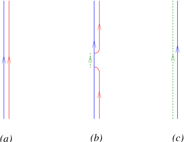
Figure 23: (a) A parallel D–string and F–string, which is not supersymmetric. (b) The F–string breaks, its ends attaching to the D-string, resulting in (c) the final supersymmetric state, a D–string with flux.

The F–string breaks, its endpoints attached to the D–string. The endpoints can then move off to infinity, leaving only the D–string behind. Of course, the D–string must now carry the charge of the F-string as well. This comes about because the F–string endpoints are charged under the D–string gauge field, so a flux runs between them; this flux remains at the end. Thus the final D–string carries both the NS–NS and R–R two–form charges. The flux is of order $g_{s}$, its energy density is of order $g_{s}$, and so the final tension is $(g_{s}^{-1}+O(g_{s}))/2\pi{\alpha^{\prime}}$. This is below the tension of the separated strings and of the same form as the BPS bound (315) for a $(1,1)$ string. A more detailed calculation shows that the final tension saturates the bound, [98] so the state is supersymmetric. In effect, the F–string has dissolved into the D–string, leaving flux behind.

We can see quite readily that this is a supersymmetric situation using T–duality. We can choose a gauge in which the electric flux is $F_{01}={\dot{A}}_{1}$. T–dualizing along the $x^{1}$ direction, we ought to get a D0–brane, which we do, except that it is moving with constant velocity, since we get ${\dot{X}}^{1}=2\pi\alpha^{\prime}{\dot{A}}_{1}$. This clearly has the same supersymmetry as a stationary D0–brane, having been simply boosted.

To calculate the number of BPS states we should put the strings in a box of length $L$ to make the spectrum discrete. For the $(1,0)$ F-string, the usual quantisation of the ground state gives eight bosonic and eight fermionic states moving in each direction for $16^{2}=256$ in all. This is the ultrashort representation of supersymmetry: half the 32 generators annihilate the BPS state and the other half generate $2^{8}=256$ states. The same is true of the $(0,1)$ D-string and the $(1,1)$ bound state just found, as will be clear from the later duality discussion of the D–string.

It is worth noting that the $(1,0)$ F–string leaves unbroken half the supersymmetry and the $(0,1)$ D–string leaves unbroken a different half of the supersymmetry. The $(1,1)$ bound state leaves unbroken not the intersection of the two (which is empty), but yet a different half. The unbroken symmetries are linear combinations of the unbroken and broken supersymmetries of the D–string.

All the above extends immediately to $p$ F–strings and one D–string, forming a supersymmetric $(p,1)$ bound state. The more general case of $p$ F-strings and $q$ D–strings is more complicated. The gauge dynamics are now non–Abelian, the interactions are strong in the infrared, and no explicit solution is known. When $p$ and $q$ have a common factor, the BPS bound makes any bound state only neutrally stable against falling apart into subsystems. To avoid this complication let $p$ and $q$ be relatively prime, so any supersymmetric state is discretely below the continuum of separated states. This allows the Hamiltonian to be deformed to a simpler supersymmetric Hamiltonian whose supersymmetric states can be determined explicitly, and again there is one ultrashort representation, $256$ states. The details, which are quite intricate, are left to the reader to consult in the literature [24, 1].

7.3 The Three–String Junction

Let us consider further the BPS saturated formula derived and studied in the two previous subsections, and write it as follows:

$$\tau_{p,q}=\sqrt{(p\tau_{1,0})^{2}+(q\tau_{0,1})^{2}}\ .$$ (319)

An obvious solution to this is

$$\tau_{p,q}\sin\alpha=q\tau_{0,1}\ ,\quad\tau_{p,q}\cos\alpha=p\tau_{1,0}\ .$$ (320)

with $\tan\alpha=q/(pg_{s})$. Recall that these are tensions of strings, and therefore we can interpret the equations (320) as balance conditions for the components of forces! In fact, it is the required balance for three strings, [113, 111] and we draw the case of $p=q=1$ in figure 24.

         

Figure 24: (a) When an F–string ends on a D–string it causes it to bend at an angle set by the string coupling. On the other side of the junction is a (1,1) string. This is in fact a BPS state. (b) Switching on some amount of the R–R scalar can vary the other angle, as shown.

Is this at all consistent with what we already know? The answer is yes. An F–string is allowed to end on a D–string by definition, and a (1,1) string is produced, due to flux conservation, as we discussed above. The issue here is just how we see that there is bending. The first thing to notice is that the angle $\alpha$ goes to $\pi/2$ in the limit of zero string coupling, and so the D–string appears in that case to run straight. This had better be true, since it is then clear that we simply were allowed to ignore the bending in our previous weakly coupled string analysis. (This study of the bending of branes beyond zero coupling has important consequences for the study of one–loop gauge theory data. [114] We shall study some of this later on.)

Parenthetically, it is nice to see that in the limit of infinite string coupling, $\alpha$ goes to $0$. The diagram is better interpreted as a D–string ending on an F–string with no resulting bending. This fits nicely with the fact that the D– and F–strings exchange roles under the strong/weak coupling duality (“S–duality”) of the type IIB string theory.

When we wrote the linearized BIon equations in section 4.6, we ignored the 1+1 dimensional case. Let us now include that part of the story here as a 1+1 dimensional gauge theory discussion. There is a flux $F_{01}$ on the world–volume, and the end of the F–string is an electric source. Given that there is only one spatial dimension, the F–string creates a discontinuity on the flux, such that e.g: [115, 50]

$$F_{01}=\left\{\matrix{g_{s}\ ,&x_{1}>0\cr 0\ ,&x_{1}<0}\right.\ ,$$ (321)

so we can choose a gauge such that

$$A_{0}=\left\{\matrix{g_{s}x^{1}\ ,&x_{1}>0\cr 0\ ,&x_{1}<0}\right.\ .$$ (322)

Just as in section 4.6, this is BPS is one of the eight scalars $\Phi^{m}$ is also switched on so that

$$\Phi^{2}(x^{1})=A_{0}\ .$$ (323)

How do we interpret this? Since $(2\pi\alpha^{\prime})\Phi^{2}$ represents the $x^{2}$ position of the D–string, we see that for $x^{1}<0$ the D–string is lying along the $x^{1}$ axis, while for $x^{1}>0$, it lies on a line forming an angle $\tan^{-1}(1/g_{s})$ with the $x^{1}$, axis.

Recall the T₁–dual picture we mentioned in the previous section, where we saw that the flux on the D–string (making the (1,1) string) is equivalent to a D0–brane moving with velocity $(2\pi\alpha^{\prime})F_{01}$. Now we see that the D0–brane loses its velocity at $x^{1}=0$. This is fine, since the apparent impulse is accounted for by the momentum carried by the F–string in the T–dual picture. (One has to tilt the diagram in order to T–dualize along the (1,1) string in order to see that there is F–string momentum.)

Since as we have seen many times that the presence of flux on the world–volume of a D$p$–brane is equivalent to having a dissolved D$(p-2)$–brane, i.e., non–zero $C_{(p-1)}$ source, we can modify the flux on the $x^{1}<0$ part of the string this way by turning on the R–R scalar $C_{0}$. This means that $\Phi^{2}(x^{1})$ will be linear there too, and so the angle $\beta$ between the D– and F–strings can be varied too (see figure 24(b)). It is interesting to derive the balance conditions from this, and then convert it into a modified tension formula, but we will not do that here. [115]

It is not hard to imagine that given the presence we have already deduced of a general $(p,q)$ string in the theory that there are three–string junctions to be made out of any three strings such that the $(p,q)$–charges add up correctly, giving a condition on the angles at which they can meet. This is harder to do in the full non–Abelian gauge theories on their world–volumes, but in fact a complete formula can be derived using the underlying $SL(2,{\hbox{{\rm Z}\kern-3.99994pt\hbox{\rm Z}}})$ symmetry of the type IIB string theory. We will have more to say about this symmetry later.

General three–string junctions have been shown to be important in a number of applications, and there is a large literature on the subject which we are unfortunately not able to review here.

7.4 $0$–$p$ Bound States

Bound states of $p$–branes and $p^{\prime}$–branes have many applications. Some of them will appear in our later lectures, and so it is worth listing some of the results here. Here we focus on $p^{\prime}=0$, since we can always reach it from a general $(p,p^{\prime})$ using T–duality.

$\bullet\quad{\mbox{\it 0--0 bound states:}}$

The BPS bound for the quantum numbers of $n$ 0–branes is $n\tau_{0}$, so any bound state will be at the edge of the continuum. What we would like to know is if there is actually a true bound state wave function, i.e., a wavefunction which is normalisable. To make the bound state counting well defined, compactify one direction and give the system momentum $m/R$ with $m$ and $n$ relatively prime. [116] The bound state now lies discretely below the continuum, because the momentum cannot be shared evenly among unbound subsystems.

This bound state problem is T–dual to the one just considered. Taking the T–dual, the $n$ D0–branes become D1–branes, while the momentum becomes winding number, corresponding to $m$ F-strings. There is therefore one ultrashort multiplet of supersymmetric states when $m$ and $n$ are relatively prime. [116] This bound state should still be present back in infinite volume, since one can take $R$ to be large compared to the size of the bound state. There is a danger that the size of the wavefunction we have just implicitly found might simply grow with $R$ such that as $R\to\infty$ it becomes non–normalisable again. More careful analysis is needed to show this. It is sufficient to say here that the bound states for arbitrary numbers of D0–branes are needed for the consistency of string duality, so this is an important problem. Some strong arguments have been presented in the literature, ($n=2$ is proven) but the general case is not yet proven. We give an embarrasingly incomplete list of papers in this topic in references. [117]

$\bullet\quad{\mbox{\it 0--2 bound states:}}$

Now the BPS bound (317) puts any bound state discretely below the continuum. One can see a hint of a bound state forming by noticing that for a coincident D0–brane and D2–brane the NS 0–2 string has a negative zero–point energy (305) and so a tachyon (which survives the GSO projection), indicating instability towards something. In fact the bound state (one short representation) is easily described: the D0–brane dissolves in the D2–brane, leaving flux, as we have seen numerous times. The brane R–R action (284) contains the coupling $C_{(1)}F$, so with the flux the D2–brane also carries the D0–brane charge. [118] There is also one short multiplet for $n$ D0–branes. This same bound state is always present when $\nu=2$.

$\bullet\quad{\mbox{\it 0--4 bound states:}}$

The BPS bound (316) makes any bound state marginally stable, so the problem is made well–defined as in the 0–0 case by compactifying and adding momentum. [119] The interactions in the action (310) are relevant in the infrared so this is again a hard problem, but as before it can be deformed into a solvable supersymmetric system. Again there is one multiplet of bound states. [119] Now, though, the bound state is invariant only under $\frac{1}{4}$ of the original supersymmetry, the intersection of the supersymmetries of the D0–brane and of the D4–brane. The bound states then lie in a short (but not ultrashort) multiplet of $2^{12}$ states.

For $2$ D0–branes and one D4–brane, one gets the correct count as follows. [120] Think of the case that the volume of the D4–brane is large. The $16$ supersymmetries broken by the D4–brane generate $256$ states that are delocalized on the D4–brane. The 8 supersymmetries unbroken by the D4–brane and broken by the D0–brane generate $16$ states (half bosonic and half fermionic), localized on the D0–brane. The total number is the product $2^{12}$. Now count the number of ways two D0–branes can be put into their $16$ states on the D4–brane: there are $8$ states with both D0–branes in the same (bosonic) state and ${\textstyle{1\over 2}}16\cdot 15$ states with the D–branes in different states, for a total of $8\cdot 16$ states. But in addition, the two–branes can bind, and there are again $16$ states where the bound state binds to the D4–brane. The total, tensoring again with the D4–brane ground states, is $9\cdot 16\cdot 256$.

For $n$ D0–branes and one D4–brane, the degeneracy $D_{n}$ is given by the generating functional  [120]

$$\sum_{n=0}^{\infty}q^{n}D_{n}\ =\ 256\ \prod_{k=1}^{\infty}\left(\frac{1+q^{k}}{1-q^{k}}\right)^{8}\ ,$$ (324)

where the term $k$ in the product comes from bound states of $k$ D0–branes then bound to the D4–brane. A recent paper discussing the D0–D4 bound state, with more references, can be found in the references. [121]

$\bullet\quad{\mbox{\it 0--6 bound states:}}$

The relevant bound is (317) and again any bound state would be below the continuum. The NS zero-point energy for 0–6 strings is positive, so there is no sign of decay. One can give D0–brane charge to the D6–brane by turning on flux, but there is no way to do this and saturate the BPS bound. So it appears that there are no supersymmetric bound states. Incidentally, and unlike the 0–2 case, the 0–6 interaction is repulsive, both at short distance and at long. [1]

$\bullet\quad{\mbox{\it 0--8 bound states:}}$

The case of the D8–brane is special, since it is rather big. It is a domain wall, since there is only one spatial dimension transverse to it. In fact, the D8–brane on its own is not really a consistent object. Trying to put it into type IIA runs into trouble, since the string coupling blows up a finite distance from it on either side because of the nature of its coupling to the dilaton. To stop this happening, one has to introduce a pair of O8–planes, one on each side, since they (for SO groups) have negative charge ($-8$ times that of the D8–brane) and can soak up the dilaton. We therefore should have 16 D8–branes for consistency, and so we end up in the type I$\prime$ theory, the T–dual of Type I. The bound state problem is now quite different, and certain details of it pertain to the strong coupling limit of certain string theories, and their “matrix” [129] formulation. [122, 123] We shall revisit this in section 8.5.

8 D–Branes, Strong Coupling, and String Duality

One of the most striking results of the middle ’90’s was the realization that all of the string theories are in fact dual to one another at strong coupling. [125, 126, 127]  This also brought eleven dimensional supergravity in the picture and started the search for M–theory, the dynamical theory within which all of those theories would fit as various effective descriptions of perturbative limits.

All of this is referred to as the “Second Superstring Revolution”. Every revolution is supposed to have a hero or heroes. We shall consider branes to be cast in that particular role, since they (and D–branes especially) supplied the truly damning evidence of the strong coupling fate of the various strign theories.

We shall discuss aspects of this in the present section. We simply study the properties of various D–branes in the various string theories, and then trust to that fact that as they are BPS states, many of these properties will survive at strong coupling.

8.1 D1–Brane Collective Dynamics

Let us first study the D1–brane. This will be appropriate to the study of type IIB and the type I string by $\Omega$–projection. Its collective dynamics as a BPS soliton moving in flat ten dimensions is captured by the 1+1 dimensional world–volume theory, with 16 or 8 supercharges, depending upon the theory we are in. (See figure 25(a).)

It is worth first setting up a notation and examining the global symmetries. Let us put the D1–brane to lie along the $x^{1}$ direction, as we will do many times in what is to come. This arrangement of branes breaks the Lorentz group up as follows:

$$SO(1,9)\supset SO(1,1)_{01}\times SO(8)_{2-9}\ ,$$ (325)

Accordingly, the supercharges decompose under (325) as

$${\bf 16}={\bf 8}_{+}+{\bf 8}_{-}$$ (326)

where $\pm$ subscripts denote a chirality with respect to $SO(1,1)$.

For the 1–1 strings, there are 8 Dirichlet–Dirichlet (DD) directions, the Neveu–Schwarz (NS) sector has zero point energy $-1/2$. The massless excitations form vectors and scalars in the 1+1 dimensional model. For the vectors, the Neumann–Neumann (NN) directions give a gauge field $A^{\mu}$. Now, the gauge field has no local dynamics, so the only contentful bosonic excitations are the transverse fluctuations. These come from the 8 Dirichlet–Dirichlet (DD) directions $x^{m}$, $m=2,\cdots,9$, and are

$$\phi^{m}(x^{0},x^{1}):\quad\lambda_{\phi}\psi^{m}_{-{1\over 2}}|0>\ .$$ (327)

The fermionic states $\xi$ from the Ramond (R) sector (with zero point energy 0, as always) are built on the vacua formed by the zero modes $\psi_{0}^{i},i{=}0,\ldots,9$. This gives the initial ${\bf 16}$. The GSO projection acts on the vacuum in this sector as:

$$(-1)^{F}=e^{i\pi(S_{0}+S_{1}+S_{2}+S_{3}+S_{4})}\ .$$ (328)

A left or right–moving state obeys $\Gamma^{0}\Gamma^{1}\xi_{\pm}=\pm\xi_{\pm}$, and so the projection onto $(-1)^{F}\xi{=}\xi$ says that left and right moving states are odd and (respectively) even under $\Gamma^{2}\ldots\Gamma^{9}$, which is to say that they are either in the ${\bf 8_{s}}$ or the ${\bf 8_{c}}$. So we see that the GSO projection simply correlates world sheet chirality with spacetime chirality: $\xi_{-}$ is in the ${\bf 8}_{c}$ of $SO(8)$ and $\xi_{+}$ is in the ${\bf 8}_{s}$.

8.2 Type IIB/Type IIB Duality

So we have seen that for a D1–brane in type IIB string theory, the right–moving spinors are in the ${\bf 8_{s}}$ of $SO(8)$, and the left-moving spinors in the ${\bf 8_{c}}$. These are the same as the fluctuations of a fundamental IIB string, in static gauge. [24] There, the supersymmetries $Q_{\alpha}$ and $\tilde{Q}_{\alpha}$ have the same chirality. Half of each spinor annihilates the F-string and the other half generates fluctuations. Since the supersymmetries have the same $SO(9,1)$ chirality, the $SO(8)$ chirality is correlated with the direction of motion.

So far we have been using the string metric. We can switch to the Einstein metric, $g_{\mu\nu}^{\rm(E)}=e^{-\Phi/2}g_{\mu\nu}^{\rm(S)}$, since in this case gravitational action has no dependence on the dilaton, and so it is an invariant under duality. The tensions in this frame are:

F–string: $$g^{1/2}_{s}/2\pi{\alpha^{\prime}}$$

D–string: $$g^{-1/2}_{s}/2\pi{\alpha^{\prime}}\ .$$ (329)

Since these are BPS states, we are able to trust these formulae at arbitrary values of $g_{s}$.

Let us see what interpretation we can make of these formulae: At weak coupling the D–string is heavy and the F–string tension is the lightest scale in the theory. At strong coupling, however, the D–string is the lightest object in the theory, (A dimensional argument shows that the lowest–dimensional branes have the lowest scale. [124]) and it is natural to believe that the theory can be reinterpreted as a theory of weakly coupled D–strings, with $g_{s}^{\prime}=g_{s}^{-1}$. One cannot prove this without a non–perturbative definition of the theory, but quantising the light D–string implies a large number of the states that would be found in the dual theory, and self–duality of the IIB theory seems by far the simplest interpretation—given that physics below the Planck energy is described by some specific string theory, it seems likely that there is a unique extension to higher energies. This agrees with the duality deduced from the low energy action and other considerations. [125, 127, 135] In particular, the NS–NS and R–R two-form potentials, to which the D– and F–strings respectively couple, are interchanged by this duality.

This duality also explains our remark about the strong and weak coupling limits of the three string junction depicted in figure 24. The roles of the D– and F–strings are swapped in the $g_{s}\to 0,\infty$ limits, which fits with the two limiting values $\alpha\to\pi/2,0$.

The full duality group of the $D=10$ Type IIB theory is expected to be $SL(2,{\hbox{{\rm Z}\kern-3.99994pt\hbox{\rm Z}}})$. [125, 127] This relates the fundamental string not only to the R–R string but to a whole set of strings with the quantum numbers of $p$ F–strings and $q$ D–strings for $p$ and $q$ relatively prime. [110] The bound states found in section 7.2 are just what is required for $SL(2,{\hbox{{\rm Z}\kern-3.99994pt\hbox{\rm Z}}})$ duality. [24] As the coupling and the R–R scalar are varied, each of these strings becomes light at the appropriate point in moduli space.

8.3 Type I/Heterotic

Let us now consider the D1–brane in the Type I theory. We must modify our previous analysis in two ways. First, we must project onto $\Omega$–even states.

As in section 2.6, the $U(1)$ gauge field $A$ is in fact projected out, since $\partial_{t}$ is odd under $\Omega$. The normal derivative $\partial_{n}$, is even under $\Omega$, and hence the $\Phi^{m}$ survive. Turning to the fermions, we see that $\Omega$ acts as $e^{i\pi(S_{1}+S_{2}+S_{3}+S_{4})}$ and so the left–moving ${\bf 8_{c}}$ is projected out and the right-moving ${\bf 8_{s}}$ survives.

Recall that D9–branes must be introduced after doing the $\Omega$ projection of the type IIB string theory. These are the $SO(32)$ Chan–Paton factors. This means that we must also include the massless fluctuations due to strings with one end on the D1-brane and the other on a D9–brane. (See figure 25(b)) The zero point energy in the NS sector for these states is $1/2$, and so there is way to make a massless state. The R sector has zero point energy zero, as usual, and the ground states come from excitations in the $x^{0},x^{1}$ direction, since it is in the NN sector that the modes are integer.

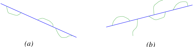
Figure 25: D1–branes (a) in Type IIB theory its fluctuations are described by 1–1 strings. (b) in Type I string theory, there are additional contributions from 1–9 strings.

The GSO projection $(-)^{F}=\Gamma^{0}\Gamma^{1}$ will project out one of these, $\lambda_{-}$, while the right moving one will remain. The $\Omega$ projection simply relates 1–9 strings to 9–1 strings, and so places no constraint on them. Finally, we should note that the 1–9 strings, as they have one end on a D9–brane, transform as vectors of $SO(32)$.

Now, by the argument that we saw in the case of the type IIB string, we should deduce that this string becomes a light fundamental string in some dual string theory at strong coupling. In these notes we have not seen such a string before. It has $(0,8$ world sheet supersymmetry, and a left moving family of 32 fermions transforming as the 32 of $SO(32)$.

Happily, there is precisely one such string theory in ten dimensions with this property. It is a closed string theory called the $SO(32)$ “heterotic” string. [17] There is in fact another ten dimensional heterotic string, with gauge group $E_{8}\times E_{8}$. It has a storng coupling limit we will examine shortly. Upon compactifying on a circle, the two heterotic string theories are perturbatively related by T–duality. [143, 144]

We have obtained the $SO(32)$ string here with the spacetime supersymmetry realized in Green–Schwarz form and with a left–moving “current algebra” in fermionic form [133], which realises a spacetime $SO(32)$ gauge symmetry. In fact, recall that we had already deduced that such a string theory might exist, by looking at the supergravity sector in section 5.4. This is just how type I/heterotic duality was deduced first [127]${}^{\!,\,}$ [135] and then D–brane constructions were used to test it more sharply [133].

Actually, heterotic string experts know that the fermionic $SO(32)$ current algebra requires a GSO projection. By considering a closed D1–brane we see that the $\Omega$ projection removes the $U(1)$ gauge field, but in fact allows a discrete gauge symmetry: a holonomy $\pm 1$ around the D1–brane. This discrete gauge symmetry is the GSO projection, and we should sum over all consistent possibilities. The heterotic strings have spinor representations of $SO(32)$, and we need to be able to make them in the Type I theory, in order for duality to be correct. In the R sector of the discrete D1–brane gauge theory, the 1–9 strings are periodic. The zero modes of the fields $\Psi^{i}$, representing the massless 1–9 strings, satisfy the Clifford algebra

$$\{\Psi^{i}_{0},\Psi^{j}_{0}\}=\delta^{ij},\qquad i,j=1,\cdots,32.$$ (330)

The quantisation now proceeds just as for the fundamental heterotic string, giving spinors ${\bf 2^{31}}+\overline{\bf 2^{31}}$, one of which is removed by the discrete gauge symmetry.

Insert 11: Dual Branes from 10D String–String Duality There is an instructive way to see how the D–string tension turns into that of an F–string. In terms of supergravity fields, part of the duality transformation involves $$G_{\mu\nu}\to e^{-{\tilde{\Phi}}}{\tilde{G}}_{\mu\nu}\ ,\quad\Phi\to-{\tilde{\Phi}}\ ,$$ where the quantities on the right, with tildes, are in the dual theory. This means that in addition to $g_{s}={\tilde{g}}_{s}^{-1}$, for the relation of the string coupling to the dual string coupling, there is also a redefinition of the string length, via $$\alpha^{\prime}={\tilde{g}}_{s}{\tilde{\alpha}}^{\prime}\ ,$$ which is the same as $$\alpha^{\prime}g_{s}={\tilde{\alpha}}^{\prime}\ .$$ Starting with the D–string tension, these relations give: $$\tau_{1}={1\over 2\pi\alpha^{\prime}g_{s}}\to{1\over 2\pi{\tilde{\alpha}}^{\prime}}=\tau^{\rm F}_{1}\ ,$$ precisely the tension of the fundamental string in the dual string theory, measured in the correct units of length. One might understandably ask the question about the fate of other D–branes. For the type IIB’s D3–brane: $$\tau_{3}={1\over(2\pi)^{3}\alpha^{\prime 2}g_{s}}\to{1\over(2\pi)^{3}{\tilde{\alpha}}^{\prime 2}{\tilde{g}}_{s}}=\tau_{3}\ ,$$ showing that the dual object is again a D3–brane. For the D5–brane, in either type IIB or type I theory: $$\tau_{5}={1\over(2\pi)^{5}\alpha^{\prime 3}g_{s}}\to{1\over(2\pi)^{5}{\tilde{\alpha}}^{\prime 3}{\tilde{g}}^{2}_{s}}=\tau^{\rm F}_{5}\ ,$$ This is the tension of a fivebrane which is not a D5–brane. This is intersting, since for both dualities, the R–R 2–form $C^{(2)}$ is exchanged for the NS–NS 2–form $B^{(2)}$, and so this fivebrane is magnetically charged under the latter. It is in fact that magnetic dual of the fundamental string. Its $g_{s}^{-2}$ behaviour identifies it as a soliton of the NS–NS fields $(G,B,\Phi)$. Continued…

Insert 11: Continued… So we conclude that there exists in both the type IIB and $SO(32)$ heterotic theories such a brane, and in fact such a brane can be constrcuted directly as a soliton solution. They should be called “F5–branes”, but this name never stuck. They go by various names like “NS5–brane” or “solitonic fivebrane”, and so on. As they are constructed completely out of closed string fields, T–duality along a direction parallel to the brane does not change its dimensionality, as would happen for a D–brane. We conclude therefore that they also exist in the T–dual Type IIA and $E_{8}\times E_{8}$ string theories. For the heterotic cases, the soliton solution also involves a background gauge field, which is in fact an instanton. We shall deduce this from duality later also, when we uncover more properties of branes within branes. One last feature worth mentioning is the worldvolume theory describing the low energy collective motions of the branes. This can be worked out directly, and string duality is consistent with the answers: From the duality, we can immediately deduce that the type IIB’s NS5–brane must have a vector multiplet, just like the D5–brane. There is non–chiral (1,1) six dimensional supersymmetry on the worldvolume. Just like with D5–branes, there is enhanced gauge symmetry when many coincide. [132] For the type IIA NS5–brane, things are different. A duality argument can be used to show that the brane actually carries a two–form potential, and so there is a six dimensional tensor multiplet on the brane. There is a chiral (0,2) supersymmetry on the brane. The gauge symmetry associated to this multiplet is also enhanced when many branes coincide. That there is either a (1,1) vector multiplet or a (0,2) tensor multiplet was first uncovered by direct analysis of the collective dynamics of the NS5–branes as solitons in the full type II theories.  [131]

8.4 Type IIA/M–Theory

In the IIA theory, the D0–brane has a mass $\tau_{0}={\alpha^{\prime}}^{-1/2}g_{s}$ in the string metric. As $g_{s}\to\infty$, this mass is the lightest scale in the theory. In addition, we have seen in section 7.4 that $n$ D0–branes have a single supersymmetric bound state with mass $n\tau_{0}$. This evenly spaced tower of states is characteristic of the appearance of an additional dimension, where the momentum (Kaluza–Klein) states have masses $n/R$ and form a continuum is $R\to\infty$. Here, $R=\alpha^{\prime 1/2}g_{s}$, so weak coupling is small $R$ and the theory is effectively ten dimensional, while strong coupling is large $R$, and the theory is eleven dimensional. We saw such Kaluza–Klein behaviour in section 3.1. The charge of the $n$th Kaluza–klein particle corresponds to $n$ units of momentum $1/R$ in the hidden dimension. In this case, this $U(1)$ is the R–R one form of type IIA, and so we interpret D0–brane charge as eleven dimensional momentum. In this way, we are led to consider eleven dimensional supergravity as the strong coupling limit of the type IIA string. This is only for low energy, of course, and the issue of the complete description of the short distance physics at strong coupling to complete the “M–theory”, is yet to be settled. It cannot be simply eleven dimensional supergravity, since that theory (like all purely field theories of gravity) is ill–defined at short distances. The most widely examined proposal for the structure of the short distance physics is “Matrix Theory”  [129], although there are other interesting proposals. [130]

It is worth noting that the existence of the bound states and of the eleventh dimension was inferred even before the significance of D–branes was understood, because they are required by lower–dimensional “U–dualities”. [126, 127]

To relate the coupling to the size of the eleventh dimension we need to compare the respective Einstein–Hilbert actions, [127]

$$\frac{1}{2\kappa_{0}^{2}g_{s}^{2}}\int d^{10}x\,\sqrt{-G_{\rm s}}R_{\rm s}=\frac{2\pi R}{2\kappa_{11}^{2}}\int d^{10}x\,\sqrt{-G_{11}}R_{11}\ .$$ (331)

The string and M theory metrics are equal up to a rescaling,

$$G_{{\rm s}\mu\nu}=\zeta^{2}G_{{\rm 11}\mu\nu}$$ (332)

and so $\zeta^{8}=2\pi R\kappa_{0}^{2}g_{s}^{2}/\kappa_{11}^{2}$. The respective masses are related $nR^{-1}=m_{11}=\zeta m_{\rm s}=n\zeta\tau_{0}$ or $R={\alpha^{\prime}}^{1/2}g_{s}/\zeta$. Combining these with the result (252) for $\kappa_{0}$, we obtain

$$\zeta=g_{s}^{1/3}\left[2^{7/9}\pi^{8/9}{\alpha^{\prime}}\kappa_{11}^{-2/9}\right]$$ (333)

and

$$R=g_{s}^{2/3}\left[2^{-7/9}\pi^{-8/9}\kappa_{11}^{2/9}\right]\ .$$ (334)

In order to emphasise the basic structure we hide in braces numerical factors and factors of $\kappa_{11}$ and ${\alpha^{\prime}}$. The latter factors are determined by dimensional analysis, with $\kappa_{11}$ having units of (M theory length^9/2) and ${\alpha^{\prime}}$ (string theory length²). We are free to set $\zeta=1$, using the same metric and units in M–theory as in string theory. In this case

$$\kappa_{11}^{2}=g_{s}^{3}\left[2^{7}\pi^{8}{\alpha^{\prime}}^{9/2}\right]\ .$$ (335)

The reason for not always doing so is that when we have a series of dualities, as below, there will be different string metrics.

For completeness, let us note that if we define Newton’s constant as before via $2\kappa_{11}^{2}=16\pi G_{N}^{11}$, then we have:

$$\kappa_{11}^{2}=2^{7}\pi^{8}\ell_{p}^{9}\ ;\quad\ell_{p}=g_{s}^{1/3}\sqrt{\alpha^{\prime}}\ ;\quad G_{N}^{11}=16\pi^{7}\ell_{p}^{9}\ .$$ (336)

It is interesting to track the eleven–dimensional origin of the various branes of the IIA theory. [118, 111, 128] The D0–branes are, as we have just seen, Kaluza-Klein states. The F1–branes, the IIA strings themselves, are wrapped membranes (“M2–branes”) of M–theory. [136] The D2–branes are membranes transverse to the eleventh dimension $X^{10}$. The D4–branes are M–theory fivebranes (“M5–branes”) [137] wrapped on $X^{10}$, while the NS (symmetric) 5–branes are M5–branes transverse to $X^{10}$. The D6–branes, being the magnetic duals of the D0–branes, are Kaluza–Klein monopoles [138] (we shall see this directly later in section 10.5). As mentioned before the D8–branes have a more complicated fate. To recap, the point is that the D8–branes cause the dilaton to diverge within a finite distance, [133] and must therefore be a finite distance from an orientifold plane, which is essentially a boundary of spacetime as we saw in section 3.9. As the coupling grows, the distance to the divergence and the boundary necessarily shrinks, so that they disappear into it in the strong coupling limit: they become part of the gauge dynamics of the nine–dimensional boundary of M–theory, [139] used to make the $E_{8}\times E_{8}$ heterotic string, to be discussed in more detail below. This raises the issue of the strong coupling limit of orientifolds in general. There are various results in the literature, but since the issue are complicated, and because the techniques used are largely strongly coupled field theory deductions, which take us well beyond the scope of these lectures, we will have to refer the reader to the literature. [209, 210, 224, 142]

One can see further indication of the eleventh dimension in the dynamics of the D2–brane. In $2+1$ dimensions, the vector field on the brane is dual to a scalar, through Hodge duality of the field strength, $*F_{2}=d\phi$. This scalar is the eleventh embedding dimension. [140, 141, 118] Carrying out the duality in detail, the D2–brane action is found to have a hidden eleven–dimensional Lorentz invariance. We shall see this feature in certain probe computations later on in section 10.5.

8.5 $E_{8}\times E_{8}$ Heterotic String/M–Theory on I

We have deduced the duals of four of the five ten dimensional string theories. Let us study the final one, the $E_{8}\times E_{8}$ heterotic string, which is T–dual to the $SO(32)$ string. [143, 144] Compactify on a large radius $R$ and turn on a Wilson line which breaks $E_{8}\times E_{8}$ to $SO(16)\times SO(16)$. This is T–dual to the $SO(32)$ heterotic string, again with a Wilson line breaking the group to $SO(16)\times SO(16)$. The couplings and radii are related

$$R^{\prime} = R^{-1}\left[{\alpha^{\prime}}\right],$$

$$g_{s}^{\prime} = g_{s}R^{-1}\left[{{\alpha^{\prime}}}^{1/2}\right]\ .$$ (337)

Now use Type I - heterotic duality to write this as a Type I theory with  [127]

$$R_{\rm I} = g_{s}^{\prime-1/2}R^{\prime}\ =\ g_{s}^{-1/2}R^{-1/2}\left[{\alpha^{\prime}}^{3/4}\right],$$

$$g_{s,{\rm I}} = g_{s}^{\prime-1}\ =\ g_{s}^{-1}R\left[{{\alpha^{\prime}}}^{-1/2}\right]\ .$$ (338)

The radius is very small, so it is useful to make another T–duality, to the ‘Type I^′’ theory. The compact dimension is then a segment of length $\pi R_{\rm I^{\prime}}$ with eight D 8–branes at each end, and

$$R_{\rm I^{\prime}} = R_{\rm I}^{-1}\left[{\alpha^{\prime}}\right]\ =\ g_{s}^{1/2}R^{1/2}\left[{\alpha^{\prime}}^{1/4}\right],$$

$$g_{s,{\rm I^{\prime}}} = g_{s,{\rm I}}R_{\rm I}^{-1}\left[2^{-1/2}{{\alpha^{\prime}}}^{1/2}\right]\ =\ g_{s}^{-1/2}R^{3/2}\left[2^{-1/2}{\alpha^{\prime}}^{-3/4}\right]\ .$$ (339)

Now take $R\to\infty$ to recover the original ten-dimensional theory (in particular the Wilson line is irrelevant and the original $E_{8}\times E_{8}$ restored). Both the radius and the coupling of the Type I^′ theory become large. The physics between the ends of the segment is given locally by the IIA string, and so the strongly coupled limit is eleven dimensional. Taking into account the transformations (332), (334), the radii of the two compact dimensions in M–theory units are

$$R_{9} = \zeta_{\rm I^{\prime}}^{-1}R_{\rm I^{\prime}}\ =\ g_{s}^{2/3}\left[2^{-11/18}\pi^{-8/9}\kappa_{11}^{2/9}\right]$$ (340)

$$R_{10} = g_{s,{\rm I^{\prime}}}^{2/3}\left[2^{-7/9}\pi^{-8/9}\kappa_{11}^{2/9}\right]\ =\ g_{s}^{-1/3}R\left[2^{-10/9}\pi^{-8/9}{\alpha^{\prime}}^{-1/2}\kappa_{11}^{2/9}\right]\ .$$

As $R\to\infty$, $R_{10}\to\infty$ also, while $R_{9}$ remains fixed and (for $g$ large) large compared to the Planck scale. Thus, in the strongly coupled limit of the ten-dimensional $E_{8}\times E_{8}$ heterotic string an eleventh dimension again appears, a segment of length $R_{9}$, with one $E_{8}$ factor on each endpoint. [139]

8.6 U–Duality

An interesting feature of string duality is the enlargement of the duality group under further toroidal compactification. There is a lot to cover, and it is somewhat orthogonal to most of what we want to do for the rest of the notes, so we will err on the side of brevity (for a change). The example of the Type II string on a five–torus $T^{5}$ is useful, since it is the setting for the simplest black hole state counting, which Amanda Peet will cover in her lectures in this school. [203]

Let us first count the gauge fields. This can be worked out simply by counting the number of ways of wrapping the metric and the various p–form potentials in the theory on the five circles of the $T^{5}$ to give a one–form in the remaining five non–compact directions. From the NS–NS sector there are 5 Kaluza–Klein gauge bosons and 5 gauge bosons from the antisymmetric tensor. There are 16 gauge bosons from the dimensional reduction of the various R–R forms: The breakdown is 10+5+1 from the forms $C^{(3)}$, $C^{(5)}$ and $C^{(1)}$, respectively. Finally, in five dimensions, one can form a two form field strength from the Hodge dual $*H$ of the 3–form field strength of the NS–NS $B_{\mu\nu}$, thus defining another gauge field.

Let us see how T–duality acts on these. The T–duality is $SO(5,5;{\hbox{{\rm Z}\kern-3.99994pt\hbox{\rm Z}}})$, as discussed in section 3.1. This mixes the first 10 NS–NS gauge fields among themselves, and the 16 R–R gauge fields among themselves, and leaves the final NS–NS field invariant. The $SO(5,5;{\hbox{{\rm Z}\kern-3.99994pt\hbox{\rm Z}}})$ representations here correspond directly to the 10, 16, and 1 of $SO(10)$.

The low energy supergravity theory for this compactification has a continuous symmetry $E_{6(6)}$ which is a non–compact version of $E_{6}$. [146] This is one of those supergravity properties that was ignored for some time, because there is no sign of it in (perturbative) string theory. But now we know better: [125] a discrete subgroup $E_{6(6)}({\hbox{{\rm Z}\kern-3.99994pt\hbox{\rm Z}}})$ is supposed to be a good symmetry of the full theory.

The gauge bosons are in the 27 of $E_{6(6)}({\hbox{{\rm Z}\kern-3.99994pt\hbox{\rm Z}}})$, which is the same as the 27 of $E_{6(6)}$. The decomposition under $SO(10)\sim SO(5,5;{\hbox{{\rm Z}\kern-3.99994pt\hbox{\rm Z}}})$ is familiar from grand unified model building,

$${\bf 27}\ \to\ {\bf 10}\ +\ {\bf 16}\ +\ {\bf 1}\ .$$ (341)

The particle excitations carrying the 10 charges are just the Kaluza–Klein and winding strings. The U–duality requires also states in the 16. These are just the various ways of wrapping Dp–branes to give D–partiles (10 for D2, 5 for D4 and 1 for D0). Finally, the state carrying the 1 charge is the NS5–brane, wrapped entirely on the $T^{5}$.

8.7 U–Duality and Bound States

It is interesting to see how some of the bound state results from the previous lecture fit the predictions of U–duality. We will generate U-transformations as a combination of T_mn⋯p, which is a T–duality in the indicated directions, and S, the IIB weak/strong transformation. The former switches between N and D boundary conditions and between momentum and winding number in the indicated directions. The latter interchanges the NS and R two-forms but leaves the R four-form invariant, and acts correspondingly on the solitons carrying these charges. We denote by ${\rm D}_{mn\cdots p}$ a D–brane extended in the indicated directions, and similarly for ${\rm F}_{m}$ a fundamental string and $p_{m}$ a momentum-carrying BPS state.

The first duality chain is

$$({\rm D}_{9},{\rm F}_{9})\ \stackrel{{\scriptstyle{\rm T}_{78}}}{{\to}}\ ({\rm D}_{789},{\rm F}_{9})\ \stackrel{{\scriptstyle\rm S}}{{\to}}\ ({\rm D}_{789},{\rm D}_{9})\ \stackrel{{\scriptstyle{\rm T}_{9}}}{{\to}}\ ({\rm D}_{78},{\rm D}_{\emptyset})\ .$$ (342)

(The last symbol denotes a D0–brane, which is of course not extended anywhere.) Thus the D–string–F–string bound state is U–dual to the 0–2 bound state.

The second chain is

$$({\rm D}_{6789},{\rm D}_{\emptyset})\ \stackrel{{\scriptstyle{\rm T}_{6}}}{{\to}}\ ({\rm D}_{789},{\rm D}_{6})\ \stackrel{{\scriptstyle\rm S}}{{\to}}\ ({\rm D}_{789},{\rm F}_{6})\ \stackrel{{\scriptstyle{\rm T}_{6789}}}{{\to}}\ ({\rm D}_{6},p_{6})\ \stackrel{{\scriptstyle\rm S}}{{\to}}\ ({\rm F}_{6},p_{6})$$ (343)

The bound states of $n$ D0–branes and $m$ D4–branes are thus U–dual to fundamental string states with momentum $n$ and winding number $m$. The bound state degeneracy (324) for $m=1$ precisely matches the fundamental string degeneracy. [147, 119, 148] For $m>1$ the same form (324) should hold but with $n\to mn$. This is believed to be the case, but the analysis (which requires the instanton picture described in the next section) does not seem to be complete. [148]

A related issue is the question of branes ending on other branes [149], and we shall see more of this later. An F–string can of course end on a D–string, so from the first duality chain it follows that a D$p$–brane can end on a D$(p+2)$–brane. The key issue is whether the coupling between spacetime forms and world–brane fields allows the source to be conserved, as with the NS–NS two–form source in figure 23. Similar arguments can be applied to the extended objects in M–theory. [149, 118]

9 D–Branes and Geometry I

9.1 D–Branes as a Probe of ALE Spaces

One of the beautiful results which we uncovered soon after constructing the type II strings was that we can “blow up” the 16 fixed points of the $T^{4}/{\hbox{{\rm Z}\kern-3.99994pt\hbox{\rm Z}}}_{2}$ “orbifold compactification” to recover string propagation on the smooth hyperKähler manifold K3. (See section 5.5.) Strictly speaking, we only recovered the algebraic data of the K3 this way, and it seemed plausible that the full metric geometry of the surface is recovered, but how can we see this directly?

We can recover this metric data by using a brane as a short distance “probe” of the geometry. This is a powerful technique, which has many useful applications as we shall see in numerous examples as we proceed.

Let us focus on a single fixed point, and the type IIB theory. The full string theory is propagating on ${\hbox{{\rm I}\kern-1.99997pt\hbox{\rm R}}}^{6}\times({\hbox{{\rm I}\kern-1.99997pt\hbox{\rm R}}}^{4}/{\hbox{{\rm Z}\kern-3.99994pt\hbox{\rm Z}}}_{2})$, which arises from imposing a symmetry under the reflection ${\bf R}:\,\,(x^{6},x^{7},x^{8},x^{9})\to(-x^{6},-x^{7},-x^{8},-x^{9})$. Now we can place a D1–brane (a “D–string”) in this plane at $x^{2},\ldots,x^{9}=0$. Here is a table to help keep track of where everything is:

	$x^{0}$	$x^{1}$	$x^{2}$	$x^{3}$	$x^{4}$	$x^{5}$	$x^{6}$	$x^{7}$	$x^{8}$	$x^{9}$
D1	$-$	$-$	$\bullet$	$\bullet$	$\bullet$	$\bullet$	$\bullet$	$\bullet$	$\bullet$	$\bullet$
ALE	$-$	$-$	$-$	$-$	$-$	$-$	$\bullet$	$\bullet$	$\bullet$	$\bullet$

(We have put the ${\hbox{{\rm I}\kern-1.99997pt\hbox{\rm R}}}^{4}/{\hbox{{\rm Z}\kern-3.99994pt\hbox{\rm Z}}}_{2}$ (ALE) space in as a ten dimensional extended object too, since it only has structure in the directions $x^{6},x^{7},x^{8},x^{9}$.)

The D1–brane can quite trivially sit at the origin and respect the symmetry ${\bf R}$, but if it moves off the fixed point, it will break the ${\hbox{{\rm Z}\kern-3.99994pt\hbox{\rm Z}}}_{2}$ symmetry. In order for it to be able to move off the fixed point there needs to be an image brane moving to the mirror image point also. We therefore need two Chan–Paton indices: one for the D–string and the other for its ${\hbox{{\rm Z}\kern-3.99994pt\hbox{\rm Z}}}_{2}$ image. So (to begin with) the gauge group carried by our D–string system living at the origin is $U(2)$, but this will be modified by the following considerations. Since ${\bf R}$ exchanges the D–string with its image, it can be chosen to act on an open string state as the exchange $\gamma=\sigma_{1}\equiv\pmatrix{0&1\cr 1&0}$. So we can write the representation of the action of ${\bf R}$ as:

$${\bf R}|{\psi,ij}\rangle = \gamma^{\phantom{-1}}_{ii^{\prime}}|{{\bf R}\psi,i^{\prime}j^{\prime}}\rangle\gamma^{-1}_{j^{\prime}j}\ ,\quad\mbox{that is,}$$

$${\bf R}|{\psi,ij}\rangle = \sigma_{ii^{\prime}}|{{\bf R}\psi,i^{\prime}j^{\prime}}\rangle\sigma^{1}_{j^{\prime}j}\ .$$ (344)

So it acts on the oscillators in the usual way but also switches the Chan–Paton factors for the brane and its image. The idea [109] is that we must choose an action of the string theory orbifold symmetry on the Chan–Paton factors when there are branes present and make sure that the string theory is consistent in that sector too. Note that the action on the Chan–Paton factors is again chosen to respect the manner in which they appear in amplitudes, just as in section 2.4.

We can therefore compute what happens: In the NS sector, the massless $\bf R$–invariant states are, in terms of vertex operators:

$$\partial_{t}X^{\mu}\sigma^{0,1},\qquad\mu=0,1$$

$$\partial_{n}X^{i}\sigma^{0,1},\qquad i=2,3,4,5$$

$$\partial_{n}X^{m}\sigma^{2,3},\qquad m=6,7,8,9.$$ (345)

The first row is the vertex operator describing a gauge field with $U(1)\times U(1)$ as the gauge symmetry. The next row constitutes four scalars in the adjoint of the gauge group, parametrising the position of the string within the six–plane ${\hbox{{\rm I}\kern-1.99997pt\hbox{\rm R}}}^{6}$, and the last row is four scalars in the “bifundamental” charges $(\pm 1,\mp 1)$ of the gauge group the transverse position on $x^{6},x^{7},x^{8},x^{9}$. Let us denote the corresponding D–string fields $A^{\mu},X^{i},X^{m}$, all $2\times 2$ matrices. We may draw a “quiver diagram” [154] displaying this gauge and matter content. (see figure 26.)

Figure 26: A diagram showing the content of the probe gauge theory. The nodes give information about the gauge groups, while the links give the amount and charges of the mattter hypermultiplets.

Such diagrams have in general an integer $m$ inside each node, representing a factor $U(m)$ in the gauge group. An arrowed edge of the diagram represents hypermultiplet transforming as the fundamental (for the sharp end) and anti–fundamental (for the blunt end) of the two gauge groups corresponding to the connected nodes. The diagram is simply a decorated version of the extended Dynkin diagram associated to $A_{1}$. This will make even more sense shortly, since there is geometric meaning to this. finally, note that one of the $U(1)$’s, (the $\sigma_{0}$ one) is trivial: nothing transforms under it, and it simply represents the overall centre of mass of the brane system.

Their bosonic action is the $d=10$ $U(2)$ Yang–Mills action, dimensionally reduced and $R$–projected (which breaks the gauge symmetry to $U(1)\times U(1))$. This dimensional reduction is easy to do. There are kinetic terms:

$$T=-{1\over 4g_{\rm YM}^{2}}\left(F^{\mu\nu}F_{\mu\nu}+\sum_{i}{\cal D}_{\mu}X^{i}{\cal D}^{\mu}X^{i}+\sum_{m}{\cal D}_{\mu}X^{m}{\cal D}^{\mu}X^{m}\right)\ ,$$ (346)

and potential terms:

$$U=-{1\over 4g_{\rm YM}^{2}}\left(2\sum_{i,m}{\rm Tr}\,[X^{i},X^{m}]^{2}+\sum_{m,n}{\rm Tr}\,[X^{m},X^{n}]^{2}\right)\ .$$ (347)

where using (274), we have $g_{\rm YM}^{2}=(2\pi)^{-1}{\alpha^{\prime}}^{-1/2}g_{s}$. (Another potentially non–trivial term disappears since the gauge group is Abelian.) The important thing to realize is that there are large families of vacua (here, $U=0$) of the theory. The space of such vacua is called the “moduli space” of vacua, and they shall have an interesting interpretation. The moduli space has two branches:

On one, the “Coulomb Branch”, $X^{m}=0$ and $X^{i}=u^{i}\sigma^{0}+v^{i}\sigma^{1}$. This corresponds to two D–strings moving independently in the ${\hbox{{\rm I}\kern-1.99997pt\hbox{\rm R}}}^{6}$, with positions $u^{i}\pm v^{i}$. The gauge symmetry is unbroken, giving independent $U(1)$’s on each D–string.

On the other, the “Higgs Branch”, $X^{m}$ is nonzero and $X^{i}=u^{i}\sigma^{0}$. The $\sigma^{1}$ gauge invariance is broken and so we can make the gauge choice $X^{m}=w^{m}\sigma^{3}$. This corresponds to the D–string moving off the fixed plane, the string and its image being at $(u^{i},\pm w^{m})$. We see that this branch has the geometry of the ${\hbox{{\rm I}\kern-1.99997pt\hbox{\rm R}}}^{6}\times{\hbox{{\rm I}\kern-1.99997pt\hbox{\rm R}}}^{4}/{\hbox{{\rm Z}\kern-3.99994pt\hbox{\rm Z}}}_{2}$ which we built in.

Now let us turn on twisted–sector fields which we uncovered in section 5.5, where we learned that they give the blowup of the geometry. They will appear as parameters in our D–brane gauge theory. Define complex $q^{m}$ by $X^{m}=\sigma^{3}{\rm Re}(q^{m})+\sigma^{2}{\rm Im}(q^{m})$, and define two doublets,

$$\Phi_{0}=\left(\begin{array}[]{c}q^{6}+iq^{7}\\ q^{8}+iq^{9}\end{array}\right),\qquad\Phi_{1}=\left(\begin{array}[]{c}\bar{q}^{6}+i\bar{q}^{7}\\ \bar{q}^{8}+i\bar{q}^{9}\end{array}\right).$$ (348)

These have charges $\pm 1$ respectively under the $\sigma^{1}$ $U(1)$. The three NS–NS moduli can be written as a vector ${\bf D}$, and the potential is proportional to

$$({\bf D}-\mbox{\boldmath$\mu$})^{2}\equiv(\Phi_{0}^{\dagger}\mbox{\boldmath$\tau$}\Phi_{0}-\Phi_{1}^{\dagger}\mbox{\boldmath$\tau$}\Phi_{1}+{\bf D})^{2}\ ,$$ (349)

where the Pauli matrices are now denoted $\tau^{I}$ to emphasise that they act in a different space. (The notation using vector $\mu$ has a significance which we shall discuss later.) This reduces to the second term of the earlier potential (347) when ${\bf D}=0$. Its form is determined by supersymmetry.

For ${\bf D}\neq 0$ the orbifold point is blown up. The moduli space of the gauge theory is simply the set of possible locations of the probe i.e., the blown up ALE space. (Note that the branch of the moduli space with $v^{i}\neq 0$ is no longer present.)

Let us count parameters and constants: The $X^{m}$ contain eight scalar fields. Three of them are removed by the ${\bf D}$–flatness condition that the potential vanish, and a fourth is a gauge degree of freedom, leaving the expected four moduli. In terms of supermultiplets, the system has the equivalent of $d=6$ $N=1$ supersymmetry. The D-string has two hypermultiplets and two vector multiplets, which are Higgsed down to one hypermultiplet and one vector multiplet.

The idea [150] is that the metric on this moduli space, as seen in the kinetic term for the D–string fields, should be the smoothed ALE metric. Given the fact that we have eight supercharges, it should be a hyperKähler manifold, [151] and the ALE space has this property. Let us explore this. [153] Three coordinates on our moduli space are conveniently defined as (there are dimensionful constants missing from this normalisation which we shall ignore for now):

$${\bf y}=\Phi_{0}^{\dagger}\mbox{\boldmath$\tau$}\Phi_{0}.$$ (350)

The fourth coordinate, $z$, can be defined

$$z=2\arg(\Phi_{0,1}\Phi_{1,1}).$$ (351)

The ${\bf D}$–flatness condition implies that

$$\Phi_{1}^{\dagger}\mbox{\boldmath$\tau$}\Phi_{1}={\bf y}+{\bf D},$$ (352)

and $\Phi_{0}$ and $\Phi_{1}$ are determined in terms of ${\bf y}$ and $z$, up to gauge choice.

The original metric on the space of hypermultiplet vevs is just the flat metric $ds^{2}=d\Phi_{0}^{\dagger}d\Phi_{0}+d\Phi_{1}^{\dagger}d\Phi_{1}$. We must project this onto the space orthogonal to the $U(1)$ gauge transformation. This is performed (for example) by coupling the $\Phi_{0},\Phi_{1}$ for two dimensional gauge fields according to their charges, and integrating out the gauge field. (This whole construction, imposing the D–flatness conditions and making the gauge identification, is known as the hyperKähler quotient. [155, 156]) The result is

$$ds^{2}=d\Phi_{0}^{\dagger}d\Phi_{0}+d\Phi_{1}^{\dagger}d\Phi_{1}-\frac{(\omega_{0}+\omega_{1})^{2}}{4(\Phi_{0}^{\dagger}\Phi_{0}+\Phi_{1}^{\dagger}\Phi_{1})}$$ (353)

with

$$\omega_{i}=i(\Phi_{i}^{\dagger}d\Phi_{i}-d\Phi_{i}^{\dagger}\Phi_{i})\ .$$ (354)

It is straightforward [153] to express the metric in terms of ${\bf y}$ and $t$ using the identity $(\alpha^{\dagger}\tau^{a}\beta)(\gamma^{\dagger}\tau^{a}\delta)=2(\alpha^{\dagger}\delta)(\gamma^{\dagger}\beta)-(\alpha^{\dagger}\beta)(\gamma^{\dagger}\delta)$ for $SU(2)$ arbitrary doublets $\alpha,\beta,\gamma,\delta$. This gives:

$$\Phi_{0}^{\dagger}\Phi_{0}=|{\bf y}|,\qquad\Phi_{1}^{\dagger}\Phi_{1}=|{\bf y}+{\bf D}|,$$

$$d{\bf y}\cdot d{\bf y}\ =\ |{\bf y}|d\Phi_{0}^{\dagger}d\Phi_{0}-\omega_{0}^{2}\ =\ |{\bf y}+{\bf D}|d\Phi_{1}^{\dagger}d\Phi_{1}-\omega_{1}^{2},$$ (355)

and we find that our metric can be written as the $N=2$ case of the Gibbons–Hawking metric:

$$ds^{2}=V^{-1}(dz-{\bf A}\cdot d{\bf y})^{2}+Vd{\bf y}\cdot d{\bf y}$$

$$V=\sum_{i=0}^{N-1}\frac{1}{|{\bf y}-{\bf y}_{i}|},\qquad\mbox{\boldmath$\nabla$}V=\mbox{\boldmath$\nabla$}\times{\bf A}\ .$$ (356)

Up to an overall normalisation (which we will fix later), we have the normalisation ${\bf y}_{0}=0$, ${\bf y}_{1}={\bf D}$, and the vector potential is

$${\bf A}({\bf y})\cdot d{\bf y}=|{\bf y}|^{-1}\omega_{0}+|{\bf y}+{\bf D}|^{-1}\omega_{1}+dz,$$ (357)

and the field strength is readily obtained by taking the exterior derivative and using the identity $\epsilon^{abc}(\alpha^{\dagger}\tau^{b}\beta)(\gamma^{\dagger}\tau^{c}\delta)=i(\alpha^{\dagger}\tau^{a}\delta)(\gamma^{\dagger}\beta)-i(\alpha^{\dagger}\delta)(\gamma^{\dagger}\tau^{a}\beta)$.

Under a change of variables, [75] this metric (for $N=2$) becomes the Eguchi–Hanson metric, 261 which we first identified as the blowup of the orbifold point. The three parameters in the vector ${\bf y}_{1}$ are the NS–NS fields representing the size and orientation of the blown up ${\hbox{{\rm I}\kern-1.99997pt\hbox{\rm P}}}^{1}$.

It is easy to carry out the generalisation to the full $A_{N-1}$ series, and get the metric (356) on the moduli space for a D1–brane probing a ${\hbox{{\rm Z}\kern-3.99994pt\hbox{\rm Z}}}_{N}$ orbifold. The gauge theory is just the obvious generalisation derived from the extended Dynkin diagram: $U(1)^{N}$, with $N+1$ bifundamental hypermultiplets with charges $(1,-1)$ under the neighbouring $U(1)$’s. (See figure 27.)

There will be $3(N-1)$ NS–NS moduli which will become the $N-1$ differences ${\bf y}_{i}-{\bf y}_{0}$ in the resulting Gibbons–Hawking metric (356). Geometrically, these correspond to the size and orientation of $N-1$ separate ${\hbox{{\rm I}\kern-1.99997pt\hbox{\rm P}}}^{1}$’s which can be blown up. In fact, we see that the there is another meaning to be ascribed to the Dynkin diagram: Each node (except the trivial one) represents a ${\hbox{{\rm I}\kern-1.99997pt\hbox{\rm P}}}^{1}$ in the spacetime geometry that the probe sees on the Higgs branch.

This entire construction which we have just described is a “hyperKähler quotient”, a powerful technique [155] for describing hyperKähler metrics of various types, and which has been used to prove the existence of the full family of ALE metrics. [156] It is remarkable that D–branes uncover the spacetime using gauge theory variables and supersymmetry to construct such a quotient, and that these are the same variables which appear in the mathematical description of the construction. We shall see this connection arising a number of other times in these notes. A reasonably elementary discussion, in this context, of the translation between D–brane physics an the mathematics of hyperKähler quotients, can be found in the literature. [157] For the full A–D–E family of ALE spaces, there is a family of “Kronheimer” gauge theories which can be derived from the A–D–E extended Dynkin diagram. (There is an excellent discussion,[63] with a stringy flavour, in the bibliography.) This is the family of gauge theories which arise on the world–volume of the D–brane probes. [154, 157] (See figure 27).

Figure 27: The extended Dynkin diagrams for the A–D–E series. As quiver diagrams, they give the gauge and matter content for the probe gauge theories which compute the resolved geometry of an ALE space. At the same time they also denote the actual underlying geometry of the ALE space, as each node denotes ${\hbox{{\rm I}\kern-1.99997pt\hbox{\rm P}}}^{1}$, with the connecting edge representing a non–zero intersection.

These families, and the correspondence to the A–D–E classification arises as follows. We start with D–branes on ${\hbox{{\rm I}\kern-1.99997pt\hbox{\rm R}}}^{4}/\Gamma$, where $\Gamma$ is any discrete subgroup of $SU(2)$ (the cover of the $SO(3)$ which acts as rotations at fixed radii). It turns out that the $\Gamma$ are classified in an “A–D–E classification”, as shown by McKay [69]. The ${\hbox{{\rm Z}\kern-3.99994pt\hbox{\rm Z}}}_{N}$ are the $A_{N-1}$ series. For the $D_{N}$ and $E_{6,7,8}$ series, we have the binary dihedral (${\hbox{{\rm I}\kern-1.99997pt\hbox{\rm D}}}_{N-2}$), tetrahedral ($\cal T$), octahedral ($\cal O$) and icosahedral ($\cal I$) groups. In order to have the D–branes form a faithful representation on the covering space of the quotient, we need to start with a number equal to the order $|\Gamma|$ of the discrete group. This was two previously, and we started with $U(2)$. So we start with a gauge group $U(|\Gamma|)$, and then project, as before.

The resulting gauge groups are given by the extended Dynkin diagrams suitably decorated. [156] (See figure 27.) For example, the simplest model in the D–series is D₄, which would require 8 D1–branes on the covering space. The final probe gauge theory after projecting is $U(2){\times}U(1)^{4}$, with four copies of a hypermultipet in the ${\bf(2,1)}$. The families of hypermultiplets (corresponding again to the links/edges in the diagram) and D–flatness conditions, etc., are precisely the variables and algebraic condition which appear in Kronheimer’s constructive proof of the existence of the ALE metrics [156, 157]. Unfortunately, it is a difficult and unsolved problem to obtain explicit metrics for the resolved spaces in the D and E cases.

9.2 Fractional D–Branes and Wrapped D–Branes

$\bullet\quad{\mbox{\it Fractional Branes}}$

Let us pause to consider the following. In the previous section, we noted that in order for the probe brane to move off the fixed point, we needed to make sure that there were enough copies of it (on the covering space) to furnish a representation of the discrete symmetry $\Gamma$ that we were going to orbifold by. After the orbifold, we saw that the Higgs branch corresponds to a single D–brane moving off the fixed point to non–zero $x^{6},x^{7},x^{8},x^{9}$. It is made up of the $|\Gamma|$ D–branes we started with on the cover, which are now images of each other under $\Gamma$. We can blow up the fixed point to a smooth surface by setting the three NS–NS fields ${\bf D}$ non–zero.

When ${\bf D}=0$, there is a Coulomb branch. There, the brane is at the fixed point $x^{6},x^{7},x^{8},x^{9}=0$. The $|\Gamma|$ D–branes are free to move apart, independently, as they are no longer constrained by $\Gamma$ projection. So in fact, we have (as many as ) $|\Gamma|$ independent branes, which therefore have the interpretation as a fraction of the full brane. None of these individual fractional branes can move off. They have charges under the twisted sector R–R fields. Twisted sector strings have no zero mode, as we have seen, and so cannot propagate.

For an arbitrary number of these fractional branes (and there is no reason not to consider any number that we want) a full $|\Gamma|$ of them must come together to form a closed orbit of $\Gamma$, in order for them to move off onto the Higgs branch as one single brane. This fits with the pattern of hypermultiplets and subsequent Higgs-ing which can take place. There simply are not the hypermultiplets in the model corresponding to the movement of an individual fractional brane off the fixed point, and so they are “frozen” there, while they can move within it, [109, 157, 160, 154] in the $x^{2},x^{3},x^{4},x^{5}$ directions.

$\bullet\quad{\mbox{\it Wrapped Branes}}$

There is further understanding of what these individual fractional branes mean. We see that when the ALE space is blown up, we fail to get the fractional branes, suggesting that there is some geometrical description to be found. The fancy language used at this point is that the Coulomb branch is “lifted”, which is to say it is no longer a branch of degenerate vacua whose existence are protected by supersymmetry. While it is possible to blow up the point with the separated fractional branes, it is not a supersymmetric operation. We shall see why presently. First, let us set up the geometry.

Recall that each node (except for the extended one) in a Dynkin diagram corresponds to a ${\hbox{{\rm I}\kern-1.99997pt\hbox{\rm P}}}^{1}$ which can be blown up in the smooth geometry. This is a cycle on which a D3–brane can be wrapped in order to make a D1–brane on ${\hbox{{\rm I}\kern-1.99997pt\hbox{\rm R}}}^{6}$. For the A_N-1–series, where things are simple, there are $N-1$ such cycles, giving that many different species of D1–brane.

Where exactly is this cycle in the metric (356)? Notice that the $4\pi$ periodic variable $z$ actually is a circle, but its radius depends upon the prefactor $V^{-1}$, which varies with ${\bf y}$ in a way which is set by the parameters (“centres”) ${\bf y}_{i}$. When ${\bf y}={\bf y}_{i}$, the $z$–circle shrinks to zero size. There is a ${\hbox{{\rm I}\kern-1.99997pt\hbox{\rm P}}}^{1}$ between successive ${\bf y}_{i}$’s, which is the minimal surface made up of the locus of $z$–circles which start out at zero size, grow to some maximum value, and then shrink again to zero size, where a ${\hbox{{\rm I}\kern-1.99997pt\hbox{\rm P}}}^{1}$ then begins again as the neighbouring cycle, having intersected with the previous one in a point. The straight line connecting this will give the smallest cycle, and so the area is $4\pi|{\bf y}_{i}-{\bf y}_{j}|$ for the ${\hbox{{\rm I}\kern-1.99997pt\hbox{\rm P}}}^{1}$ connecting centres ${\bf y}_{i,j}$.

If a brane is wrapped on a cycle, it cannot be pulled off (by definition), even after the cycle has shrunken to zero size. Is this perhaps responsible for the fractional brane description? If we can get it to work for a single cycle [153, 167] (we need to get rid of the total D3–brane charge), we can get it to work for the entire A–D–E series of ALE spaces: the general Dynkin diagrams telling us about the underlying geometry all have the interpretation as the family of blown up cycles.

Here is one way to do it: [168] Imagine a D3–brane with some non–zero amount of $B+2\pi\alpha^{\prime}F$ on its world volume. Recall that this corresponds to some D1–brane dissolved into the worldvolume. We deduced this from T–duality in earlier sections. (We did it with pure $F$, but we can always gauge in some $B$.) Since we need a total D3–brane charge of zero in our final solution, let us also consider a D3–brane with opposite charge, and with some non–zero $B+2\pi\alpha^{\prime}{\widetilde{F}}$ on its worldvolume. We write $\widetilde{F}$ to distinguish it from the $F$ on the other brane’s worldvolume, but the $B$’s are the same, since this is a spacetime background field. So we have a worldvolume interaction:

$$\mu_{3}\int C^{(2)}\wedge\left\{(B+2\pi\alpha^{\prime}F)-(B+2\pi\alpha^{\prime}{\widetilde{F}})\right\}\ ,$$ (358)

where we are keeping the terms separate for clarity. Our net D3–brane charge is zero. Now let us choose $2\pi\alpha^{\prime}(\int_{\Sigma}{F}-{\widetilde{F}})={\mu_{1}/\mu_{3}}$, and $\Phi_{B}\equiv({\mu_{3}/\mu_{1}})\int_{\Sigma}{B}=1/2$ for some two dimensional spatial subspace $\Sigma$ of the 3–volume. (Note that $\Phi_{B}\sim\Phi_{B}+1$.) are only This gives a net D1–brane charge of $1/2+1/2=1$. The two halves shall be our fractional branes. Right now, they are totally delocalized in the world–volume of the D3–anti D3 system. We can make the D1’s more localised by identifying $\Sigma$ (the parts of the 3–volume where $B$ and $F$ are non–zero) with the ${\hbox{{\rm I}\kern-1.99997pt\hbox{\rm P}}}^{1}$ of the ALE space. The smaller the ${\hbox{{\rm I}\kern-1.99997pt\hbox{\rm P}}}^{1}$ is, the more localized the D1’s are. In the limit where it shrinks away we have the orbifold fixed point geometry. (Note that we still have $\Phi_{B}=1/2$ on the shrunken cycle. Happily, this is just the value needed to be present for a sensible conformal field theory description of the orbifold sector. [71])

Once the D1’s are completely localized in $x^{6},x^{7},x^{8},x^{9}$ from the shrinking away of the ${\hbox{{\rm I}\kern-1.99997pt\hbox{\rm P}}}^{1}$, then they are free to move supersymmetrically in the $x^{2},x^{3},x^{4},x^{5}$ directions. This should be familiar as the general facts we uncovered about the D$p$–D$(p+2)$ bound state system: If the D$(p+2)$ is extended, the D$p$ cannot move out of it and preserve supersymmetry. This is also T–dual to a single brane at an angle and we shall see this next.

9.3 Wrapped, Fractional and Stretched Branes

There is yet another useful way of thinking of all the of the above physics, and even more aspects of it will become manifest here. It requires exploring a duality to another picture altogether. This duality is morally a T–duality, although since it is a non–trivial background that is involved, we should be careful. It is best trusted at low energy, as we cannot be sure that the string theories are completely dual at all mass levels. So we should probably claim only that the backgrounds give the same low energy physics. Nevertheless, once we arrive at our goal, we can forget about where it came from and construct it directly in its own right.

Up to a change of variables, in the supergravity background (356), ${\bf y}$ can be taken to be the vector ${\bf y}=(x^{7},x^{8},x^{9})$ while we will take $x^{6}$ to be our periodic coordinate $z$. (There are some dimensionful parameters which were left out of the derivation of (356), for clarity, and we shall put them in by hand, and try to fix the pure numbers with T–duality.)

Then, using the T–duality rules (140) we can arrive at another background: (note that we have adjoined the flat transverse spacetime ${\hbox{{\rm I}\kern-1.99997pt\hbox{\rm R}}}^{6}$ to make a ten dimensional solution, and restored an $\alpha^{\prime}$ for dimensions):

$$ds^{2} = -dt^{2}+\sum_{m=1}^{5}dx^{m}dx^{m}+V(y)(dx^{6}dx^{6}+d{\bf y}\cdot d{\bf y})$$

$$e^{2\Phi} = V(y)=\sum_{i=0}^{N-1}{\sqrt{\alpha^{\prime}}\over|{\bf y}-{\bf y}_{i}|}\ ,$$ (359)

which is also a ten dimensional solution if taken with a non–trivial background field [169, 170] $H_{mns}=\epsilon_{mns}^{\phantom{mns}r}\partial_{r}\Phi$ which defines the potential $B_{6i}$ ($i=7,8,9$) as a vector $A_{i}$ which satisfies $\nabla V=\nabla{\times}{\bf A}$. Non–zero $B_{6i}$ arose because the T–dual solution had non zero $G_{6i}$.

In fact, this is not quite the solution we are looking for. What we have arrived at is a solution which is independent of the $x^{6}$ direction. This is neccessary if we are to use the operation (140). In fact, we expect that the full solution we seek has some structure in $x^{6}$, since translation invariance is certainly broken there. This is because the $x^{6}$–circle of the ALE space has $N$ places where winding number can change, since the circle shrinks away there. So we expect that the same must be true for momentum in the dual situation. [171] A simple guess for a solution which is localised completely in the $x^{6},x^{7},x^{8},x^{9}$ directions is to simply as that it be harmonic there. We simply take ${\bf x}=(x^{6},{\bf y})$ to mean a position in the full ${\hbox{{\rm I}\kern-1.99997pt\hbox{\rm R}}}^{4}$, and replace $V(y)$ by:

$$V(x)=1+\sum_{i=0}^{N-1}{{\alpha^{\prime}}\over({\bf x}-{\bf x}_{i})^{2}}$$ (360)

We have done a bit more than just delocalized. By adding the 1 we have endowed the solution with asymptotically flat behaviour. However, adding the 1 is consistent with $V({\bf x})$ being harmonic in $x^{6},x^{7},x^{8},x^{9}$, and so it is still a solution.

The solution we have just uncovered is made up of a chain of $N$ objects which are pointlike in ${\hbox{{\rm I}\kern-1.99997pt\hbox{\rm R}}}^{4}$ and magnetic sources of the NS–NS potential $B_{\mu\nu}$. They are in fact the “NS5–branes” we discovered by various arguments in previous sections, and a derivation of the solution using S–duality transformations is presented in insert 13 (p.10.1), with the result (394). Here, the NS5–branes are arranged in a circle on $x^{6}$, and distributed on the rest of ${\hbox{{\rm I}\kern-1.99997pt\hbox{\rm R}}}^{4}$ according to the centres ${\bf x}_{i}$, $i=0,\cdots,N-1$.

Recall that we had a D1–brane lying along the $x^{1}$ direction, probing the ALE space. By the rules of T–duality on a D–brane, it becomes a D2–brane probing the space, with the extra leg of the D2–brane extended along the compact $x^{6}$ direction. The D2–brane penetrates the two NS5–branes as it winds around once. The point at which it passes through an NS5–brane is given by four numbers ${\bf x}_{i}$ for the $i$th brane. The intersection point can be located anywhere within the fivebrane’s worldvolume in the directions $x^{2},x^{3},x^{4},x^{5}$. (See figure 28(a).)

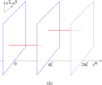
Figure 28: (a) This configuration of two NS5–branes on a circle with D2–branes streched between them is dual to a D1–brane probing an A₁ ALE space. (b) The Coulomb branch where the D2–brane splits into two “fractional branes”.

In the table below, we show the extension of the D2 in the $x^{6}$ direction as a $|-|$ to indicate that it may be of finite extent, if it were ending on an NS5–brane.

	$x^{0}$	$x^{1}$	$x^{2}$	$x^{3}$	$x^{4}$	$x^{5}$	$x^{6}$	$x^{7}$	$x^{8}$	$x^{9}$
D2	$-$	$-$	$\bullet$	$\bullet$	$\bullet$	$\bullet$	$|-|$	$\bullet$	$\bullet$	$\bullet$
NS5	$-$	$-$	$-$	$-$	$-$	$-$	$\bullet$	$\bullet$	$\bullet$	$\bullet$

This arrangement, with the branes lying in the directions which we have described, preserves the same eight supercharges we discussed before. Starting with the 32 supercharges of the type IIA supersymmetry, the NS5–branes break a half, and the D2–brane breaks half again. The infinite part of the probe, an effective one–brane (string), has a $U(1)$ on its worldvolume, and its tension is $\mu=2\pi\ell\mu_{2}$, where $\ell$ is the as yet unspecified length of the new $x^{6}$ direction. Note that if $\ell=\sqrt{\alpha^{\prime}}$, we get the tension of a D1–brane, which apparently fixes all of our parameters in the T–dual model in terms of the ALE space. 

Let us focus on $N=2$. If the two fivebranes (with positions ${\bf x}_{1},{\bf x}_{2}$; we can set ${\bf x}_{0}$ to zero) are located at the same ${\bf y}=(x^{7},x^{8},x^{9})$ position, then the D2–brane can break into two segments, giving a $U(1)\times U(1)$ (one from each segment) on the 1–brane part stretched in the infinite $x^{1}$ direction. The two segments can move independently within the NS5–brane worldvolume, while still remaining parallel, preserving supersymmetry. 

This is the precise analogue of the Coulomb branch of the D1–brane probing the ALE space that we saw earlier! The hypermultiplets of the $U(1)\times U(1)$ theory are made here by stretching fundamental strings across the NS5–branes in $x^{6}$ to make a connection between the D–brane segments. [172] The three differences ${\bf y}_{1}-{\bf y}_{2}$ are the T–dual of the NS–NS parameters representing the size and orientation of the ALE space’s ${\hbox{{\rm I}\kern-1.99997pt\hbox{\rm P}}}^{1}$. The $x^{6}$ separation of the NS5–branes is dual to the flux $2\pi\ell\Phi_{B}$. This is the length of one segment while $2\pi\ell(1-\Phi_{B})$ is the length of the other. (This fits with the fact that $\Phi_{B}\sim\Phi_{B}+1$.) Notice also that there is an interesting duality between the quiver diagram and the arrangement of branes in the dual picture. (See figure 29.)

Figure 29: There is a duality between the extended Dynkin diagram which gives the probe gauge theory and the diagram representing D–branes stretched between NS5–branes. The nodes in one are replaced by links in the other. In particular, the number inside the Dynkin nodes become the number of D–branes in the links in the dual diagram. The hypermultiplets associated with links in the Dynkin diagram arise from strings connecting the D–brane fragment ending on one side of an NS5–brane with the fragment on the other.

The original setup had the lengths equal, but we can change them at will, and this is dual to changing $\Phi_{B}$. Note the possibility of one of the lengths becoming zero. The NS–branes become coincident, and at the same time a fractional brane becomes a tensionless string, and we get an $A_{1}$ enhancement of the gauge symmetry carried by the two–form potential which lives on the type IIA NS5–brane. [132] If we had D1–branes stretched between NS5’s in type IIB instead, we would get massless particles, and an enhanced $SU(2)$ gauge symmetry. (See insert 11 (p.8.3))

If the segments are separated, and thus attached to the NS5–branes, then when we move the NS5–branes out to different $x^{789}$ positions, the segments must tilt in order to remain stretched between the two branes. They will therefore be oriented differently from each other and will break supersymmetry. This is how the Coulomb branch is “lifted” in this language. (See figure 30(c)) A segment at orientation gives a contribution $\sqrt{(2\pi\ell\Phi_{B})^{2}+({\bf y}_{1}-{\bf y}_{2})^{2}}$ to the D1–brane’s tension. This formula should be familiar: it is of the form for the more general formula for a bound state of a D1–D3 bound state, to which this tilted D2–brane segment is dual.

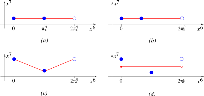
Figure 30: Possible deformations of the brane arrangements, and their gauge theory interpretation: (a) The configuration dual to the standard orbifold limit with the traditional “half unit” of B–flux; (b) Varying the distribution of B–flux between segments. Sending it to zero will make the NS5–brane coincide and give an enhanced gauge symmetry; (c) Switching on a deformation parameter (an FI term in gauge theory) “lifts” the Coulomb branch: if there are separated D–brane fragments, supersymmetry cannot be retained; (d) First Higgs-ing to make a complete brane allows smooth movement onto the supersymmetric Higgs branch.

For supersymmetric vacua to be recovered when the NS–fivebrane are moved to different positions (the dual of smoothing the ALE space) the branes segments must first rejoin with the other (Higgs–ing), giving the single D–brane. Then it need not move with the NS5–branes as they separate in ${\bf y}$, and can preserve supersymmetry by remaining stretched as a single component. (See figure 30(d)) Its ${\bf y}$ position and an $x^{6}$ Wilson line constitute the Higgs branch parameters. Evidently the metric on these Higgs branch parameters is that of an ALE space, since the 1+1 dimensional gauge theory is the same as the discussion in section 9.1, and hence the moduli spaces match. It is worth sharpening this into a field theory proof of the low energy validity of the T–duality, but we will not do that here.

It is worth noting here that once we have uncovered the existence of fractional D–branes with a modulus for their separation, there is no reason why we cannot separate them infinitely far from each other and consider them in their own right. We also have the right to take a limit where we focus on just one segment with a finite separation between two NS5–branes, but with a non–compact $x^{6}$ direction. This is achievable from what we started with here by sending $\Phi_{B}\to 0$, but changing to scaled variables in which there is still a finite separation, and hence a finite gauge coupling on the brane segment in question. (U–duality will then give us various species of branes ending on branes which we will discuss later.)

Fractional branes, and their duals the stretched brane segments, are useful objects since they are less mobile than a complete D–brane, in that they cannot move in some directions. One use of this is of course the study of gauge theory on branes with a reduced number of supersymmetries and a reduced number of charged hypermultiplets. [172, 178] This has a lot of applications, (there are reviews available [179, 180, 181]), some of which we will consider later.

9.4 D–Branes as Instantons

Consider a D0–brane and $N$ coincident D4–branes. There is a $U(1)$ on the D0 and $U(N)$ on the D4’s, which we shall take to be extended in the $x^{6},x^{7},x^{8},x^{9}$ directions. The potential terms in the action are

$$\frac{\chi_{i}^{\dagger}\chi_{i}}{(2\pi{\alpha^{\prime}})^{2}}\sum_{a=1}^{5}(X_{a}-Y_{a})^{2}+\frac{1}{4g_{0}^{2}}\sum_{I=1}^{3}(\chi_{i}^{\dagger}\tau^{I}\chi_{i})^{2}\ .$$ (361)

Here $a$ runs over the dimensions transverse to the D4–brane, and $X_{a}$ and $Y_{a}$ are respectively the D0–brane and D4–brane positions, and for now we ignore the position of the D0–brane within the D4–branes’ worldvolume. This is the same action as in the earlier case (310), but here the D4–branes have infinite volume and so their $D$–term drops out. We have also written the 0–4 hypermultiplet field $\chi$ with a D4–brane index $i$. (The $SU(2)_{R}$ index is suppressed). The potential (361) is exact on grounds of ${\cal N}{=}2$ supersymmetry. The first term is the ${\cal N}{=}2$ coupling between the hypermultiplets $\chi$ and the vector multiplet scalars $X$, $Y$. The second is the $U(1)$ $D$–term.

For $N>1$ there are two branches of moduli space, in direct analogy with the ALE case. The Coulomb branch is $(X\neq Y,\quad\chi=0)$, which is simply the position of the D0–brane transverse to the D4–branes. There is a mass for $\chi$ and so its vev is zero. The Higgs branch $(X=Y,\quad\chi\neq 0)$ represents the physics of the D0–brane being stuck on the world–volume of the D4–branes. The non–zero vev of $\chi$ Higgses away the $U(1)$ and some of the $U(N)$.

Let us count the dimension of moduli space. There are $4N$ real degrees of freedom in $\chi$. The vanishing of the $U(1)$ $D$–term imposes three constraints, and modding by the (broken) $U(1)$ removes another degree of freedom leaving $4N-4$. There are 4 moduli for the position of the D0–brane inside the the D4–branes, giving a total of $4N$ moduli. This is in fact the correct dimension of moduli space for an $SU(N)$ instanton when we do not mod out also the $SU(N)$ identifications. For $k$ instantons this dimension becomes $4Nk$.

Another clue that the Higgs branch describes the D0–brane as a D4–brane gauge theory instanton is the fact that the Ramond–Ramond couplings include a term $\mu_{4}C_{(1)}\wedge{\rm Tr}(F{\wedge}F)$. As shown in section 6.2, when there is an instanton on the D4–brane it carries D0–brane charge. The position of the instanton is given by the 0–0 fields, while the 0–4 should give the size and shape. (See figure 31).

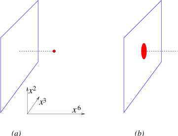
Figure 31: Instantons and the D$p$–D$(p+4)$ system. (a) The Coulomb branch of the D$p$–brane theory represents a pointlike brane away from the D$(p+4)$–brane. (b) The Higgs branch corresponds to it being stuck inside the D$(p+4)$–brane as a finite sized instanton of the D$(p+4)$–brane’s gauge theory.

The connection between D–branes and instantons was found first in the case $(p,p^{\prime})=(9,5)$ by Witten. [108] This situation is T–dual to the case we are discussing here, but does not have the Coulomb branch, since the D9–branes fill spacetime. The realization that an instanton of D$p$–brane gauge theory can shrink to zero size and move off as a D$(p-4)$–brane was noted by Douglas. [150]

9.5 Seeing the Instanton with a Probe

Actually, we can really see the resulting instanton gauge fields by using a D1–brane as a probe of the D9–D5 system. [150] It breaks half of the supersymmetries left over from the 9–5 system, leaving four supercharges overall. The effective 1+1 dimensional theory is $(0,4)$ supersymmetric and is made of 1–1 fields, which has two classes of hypermulitplets. One represents the motions of the probe transverse to the D5, and the other parallel. The 1–5 and 1–9 fields are also hypermultiplets, while the 9–5 and 5–5 fields are parameters in the model.

Let us place the D5–branes such that they are pointlike in the $x^{6},x^{7},x^{8},x^{9}$ directions. The D1–brane probe will lie along the $x^{1}$ direction, as usual.

	$x^{0}$	$x^{1}$	$x^{2}$	$x^{3}$	$x^{4}$	$x^{5}$	$x^{6}$	$x^{7}$	$x^{8}$	$x^{9}$
D1	$-$	$-$	$\bullet$	$\bullet$	$\bullet$	$\bullet$	$\bullet$	$\bullet$	$\bullet$	$\bullet$
D5	$-$	$-$	$-$	$-$	$-$	$-$	$\bullet$	$\bullet$	$\bullet$	$\bullet$

This arrangement of branes breaks the Lorentz group up as follows:

$$SO(1,9)\supset SO(1,1)_{01}\times SO(4)_{2345}\times SO(4)_{6789}\ ,$$ (362)

where the superscripts denote the sub–spacetimes in which the surviving factors act. We may label [173, 150] the worldsheet fields according to how they transform under the covering group:

$$[SU(2)^{\prime}\times\widetilde{SU(2)}^{\prime}]_{2345}\times[SU(2)_{R}\times SU(2)_{L}]_{6789}\ ,$$ (363)

with doublet indices $(A^{\prime},\tilde{A}^{\prime},A,Y)$, respectively.

The analysis that we did for the D1–brane probe in the type I string theory in section 8.3 still applies, but there are some new details. Now $\xi_{-}$ is further decomposed into $\xi^{1}_{-}$ and $\xi^{2}_{-}$, where superscripts 1 and 2 denote the decomposition into the (2345) sector and the (6789) sector, respectively. So we have that the fermion $\xi^{1}_{-}$ (hereafter called $\psi_{-}^{A\tilde{A}^{\prime}}$) is the right–moving superpartner of the four component scalar field $b^{A^{\prime}\tilde{A}^{\prime}}$, while $\xi^{2}_{-}$ (called $\psi_{-}^{A^{\prime}Y}$) is the right–moving superpartner of $b^{AY}$. The supersymmetry transformations are:

$$\delta b^{A^{\prime}\tilde{A}^{\prime}}=i\epsilon_{AB}\eta^{A^{\prime}A}_{+}\psi_{-}^{B\tilde{A}^{\prime}}$$

$$\delta b^{AY}=i\epsilon_{A^{\prime}B^{\prime}}\eta^{AA^{\prime}}_{+}\psi_{-}^{B^{\prime}Y}\ .$$ (364)

In the 1–5 sector, there are four DN coordinates, and four DD coordinates giving the NS sector a zero point energy of 0, with excitations coming from integer modes in the $2345$ directions, giving a four component boson. The R sector also has zero point energy of zero, with excitations coming from the 6789 directions, giving a four component fermion $\chi$.

The GSO projections in either sector reduce us to two bosonic states $\phi^{A^{\prime}}$ in and decomposes the spinor $\chi$ into left and right moving two component spinors, $\chi_{-}^{A}$ and $\chi_{+}^{Y}$, respectively. We see that $\chi_{-}^{A}$ is the right–moving superpartner of $\phi^{A^{\prime}}$. Taking into account the fact that there is a D5–brane index for these fields, we can display the components $(\phi^{A^{\prime}m},\chi_{-}^{Am})$ which are related by supersymmetry:

$${\delta\phi^{A^{\prime}m}=i\epsilon_{AB}\eta^{A^{\prime}A}_{+}\chi_{-}^{Bm}.}$$ (365)

and the $(0,4)$ supersymmetry parameter is denoted by $\eta_{+}^{A^{\prime}A}$. Here, $m$ is a D5–brane group theory index. Also, $\chi_{+}^{Y}$ has components $\chi_{+}^{Ym}$.

The supersymmetry transformation relating them to the left moving fields are:

$$\delta\lambda_{+}^{M}=\eta_{+}^{AA^{\prime}}C^{M}_{AA^{\prime}}$$

$$\delta\chi_{+}^{Ym}=\eta_{+}^{AA^{\prime}}C^{Ym}_{AA^{\prime}}\ ,$$ (366)

where $C^{M}_{AA^{\prime}}$ and $C^{Ym}_{AA^{\prime}}$ shall be determined shortly. They will be made of the bosonic 1–1 fields and other background couplings built out of the 5–5 and 5–9 fields.

The 5–5 and 5–9 couplings descend from the fields in the D9–D5 sector. There are some details of those fields which are peculiarities of the fact that we are in type I string theory. First, the gauge symmetry on the D9–branes is $SO(32)$. Also, for $k$ coincident D5–branes, there is a gauge symmetry $USp(2k)$, [108] since there is an extra $-1$ in the action of $\Omega$ on D5–brane fields.  [109] The 5–5 sector hypermultiplet scalars (fluctuations in the transverse $x^{6,7,8,9}$ directions) transform in the antisymmetric of $USp(2k)$, which we call $X^{AY}_{mn}$, matching the notation in the literature.  [150] Meanwhile, the 5–9 sector produces a $\bf{(2k,32)}$, denoted $h^{Am}_{M}$, with $m$ and $M$ as in D5– and D9–brane labels.

Using the form of the transformations (366) allows us to write the non–trivial part of the $(0,4)$ supersymmetric 1+1 dimensional Lagrangian containing the Yukawa couplings and the potential of the $(0,4)$ model:

$${\cal L}_{\rm tot}={\cal L}_{\rm kinetic}-{i\over 4}\int d^{2}\!\sigma\biggl{[}\lambda_{+}^{M}\left(\epsilon^{BD}{\partial C^{M}_{BB^{\prime}}\over\partial b^{DY}}\psi_{-}^{B^{\prime}Y}+\epsilon^{B^{\prime}D^{\prime}}{\partial C^{M}_{BB^{\prime}}\over\partial\phi^{D^{\prime}m}}\chi_{-}^{Bm}\right)\biggr{.}$$

. $$\hskip 85.35826pt+\chi_{+}^{Ym}\left(\epsilon^{BD}{\partial C^{Ym}_{BB^{\prime}}\over\partial b^{DY}}\psi_{-}^{B^{\prime}Y}+\epsilon^{B^{\prime}D^{\prime}}{\partial C^{Ym}_{BB^{\prime}}\over\partial\phi^{D^{\prime}m}}\chi_{-}^{Bm}\right)\biggr{.}$$

. $$\hskip 85.35826pt+{1\over 2}\epsilon^{AB}\epsilon^{A^{\prime}B^{\prime}}\left(C^{M}_{AA^{\prime}}C^{M}_{BB^{\prime}}+C^{Ym}_{AA^{\prime}}C^{Ym}_{BB^{\prime}}\right)\biggr{]}.$$ (367)

This is the most general [173] $(0,4)$ supersymmetric Lagrangian with these types of multiplets, providing that the $C$ satisfy the condition:

$${C^{M}_{AA^{\prime}}C^{M}_{BB^{\prime}}+C^{Ym}_{AA^{\prime}}C^{Ym}_{BB^{\prime}}+C^{M}_{BA^{\prime}}C^{M}_{AB^{\prime}}+C^{Ym}_{BA^{\prime}}C^{Ym}_{AB^{\prime}}=0\ ,}$$ (368)

where ${\cal L}_{\rm kinetic}$ contains the usual kinetic terms for all of the fields. Notice that the fields $b^{A^{\prime}{\tilde{A}}^{\prime}}$ and $\psi_{-}^{AA^{\prime}}$ are free.

Now equation (367) might appear somewhat daunting, but is in fact mostly notation. The trick is to note that general considerations can allow us to fix what sort of things can appear in the matrices $C_{AA^{\prime}}$. The distance between the D1–brane and the D5–branes should set the mass of the 1–5 fields, $\phi^{A^{\prime}m}$ and its fermionic partners $\chi^{Am}_{-},\chi^{Ym}_{+}$. So there should be terms of the form:

$$\phi_{A^{\prime}}^{m}\phi^{A^{\prime}n}(X^{AY}_{mn}-b^{AY}\delta_{mn})^{2}\ ,\quad\chi^{Am}_{-}\chi^{Yn}_{+}(X^{AY}_{mn}-b^{AY}\delta_{mn})\ ,$$ (369)

where the term in brackets is the unique translation invariant combination of the appropriate 1–1 and 5–5 fields. There are also 1–5–9 couplings, which would be induced by couplings between 1–9, 1–5 and 5–9 fields, in the form $\lambda^{M}_{+}\chi^{A}_{m-}h^{m}_{AM}$.

In fact, the required $C$’s which satisfy the requirements (368) and give us the coupling which we expect are: [150]

$$C^{M}_{AA^{\prime}}=h_{A}^{Mm}\phi_{A^{\prime}m}$$

$$C^{Ym}_{AA^{\prime}}=\phi_{A^{\prime}}^{n}(X^{Ym}_{An}-b_{A}^{Y}\delta_{n}^{m})\ .$$ (370)

The $(0,4)$ conditions (368) translate directly into a series of equations for the D5–brane hypermultiplets to act as data specifying an instanton via the “ADHM description”. [174] The crucial point is [173] that the vacua of the sigma model gives a space of solutions which is isomorphic to those of ADHM.

One can see that one has the right number of parameters as follows: The potential is of the form $V=\phi^{2}((X-b)^{2}+h^{2})$. So the term in brackets acts as a mass term for $\phi$. The potential vanishes for $\phi=0$, leaving this space of vacua to be parametrized by $X$ and $h$, with $b$ giving the position of the D1–brane in the four transverse directions. Let us write ${\widehat{X}}^{AY}{=}(X^{AY}{-}b^{AY})$ as the centre of mass field.

Notice that for these vacua ($\phi=0$), the Yukawa couplings are of the form $\sum_{a}\lambda^{a}_{+}B^{a}_{Am}\chi_{-}^{Am}$ where $B^{a}_{Am}=\partial C^{a}_{AB^{\prime}}/\partial\phi_{B^{\prime}m}$, and the index $a$ is the set $(M,Y,m)$. There are 4$k$ fermions in $\chi_{-}$ and so this pairs with 4$k$ fermions in the set $\lambda^{a}_{+}=(\chi_{+}^{Ym},\lambda^{M}_{+})$, leaving a subspace of 32 massless modes describing the non–trivial gauge bundle.

The idea is to write the low energy sigma model action for these massless fields. This is done as follows: a basis of massless components is given by $v_{i}^{a}$ ($i=1,\cdots,32$) defined by $\sum_{a}v_{v}^{a}B^{a}_{Am}=0$, and we choose it to be orthonormal: $\sum_{a}v_{i}^{a}v_{j}^{a}=\delta_{ij}$. The basis $v^{a}_{i}$ depends on ${\widehat{X}}$. So substituting $\lambda^{a}_{+}=\sum_{i}v_{i}^{a}\lambda^{i}_{+}$ into the kinetic energy gives: [173]

$$\lambda^{a}_{+}\partial_{-}\lambda^{a}_{+}=\sum_{i,j}\biggl{\{}\lambda_{+i}\left(\delta_{ij}\partial_{-}+\partial_{-}{\widehat{X}}^{\mu}A_{\mu,ij}\right)\lambda_{+j}\biggr{\}}\ ,$$ (371)

where

$$A_{\mu,ij}\equiv A_{BY,ij}=\sum_{a}v^{a}_{i}{\partial v_{j}^{a}\over\partial{\widehat{X}}^{BY}}$$ (372)

we have used the $x^{6},x^{7},x^{8},x^{9}$ spacetime index $\mu$ on our 1–1 field ${\widehat{X}}^{BY}$ instead of the indices $(B,Y)$, for clarity.

So we see that the second term in (371) shows the sigma model couplings of the fermions to a background gauge field $A_{\mu}$. Since we have generically

$$B^{a}_{Am}:\quad\left({\widehat{X}}^{AY},h^{Mm}_{A}\right)\ ,$$ (373)

the orthonormal basis $v^{a}_{i}$ is

$$v^{a}:\quad\left({h^{Mm}_{A}\over\sqrt{{\widehat{X}}^{2}+h^{2}}},{-{\widehat{X}}^{AY}\over\sqrt{{\widehat{X}}^{2}+h^{2}}}\right)\ ,$$ (374)

and from (372), it is clear that the background gauge field is indeed of the form of an instanton: The 5–9 field $h$ indeed sets the scale size of the instanton, and the 5–5 field $X$ sets its position. Notice that this model gives a meaning to the instanton even when its size drops to zero, well below any field theory or string theory scale in the problem. This is another sign that D–branes are able to see small “substringy” scales where new physics is to be found. [86, 87, 88] In the D$p$–D$(p+4)$ description, zero scale size is the place where the Higgs branch joins onto the Coulomb branch representing the D$p$–brane becoming pointlike (getting an enhanced gauge symmetry on its worldvolume), and moves out of the worldvolume of the brane. (For $p=5$ this branch is not present.)

Insert 12: The Heterotic NS5–brane Recall that in insert 11 (p.8.3) we deduced that there must be a solitonic brane, the NS5–brane, which lives in $SO(32)$ heterotic string theory. This followed from the fact the D5–brane of type I had to map to such an object. This heterotic version of the NS5–brane inherits a number of properties from the D5–brane, the prinicipal one being that it must be an instanton of the $SO(32)$ gauge theory of the heteroic string. In fact, it is the instanton property which led to its discovery early on. As a solution, it looks like the following (to leading order in ${\alpha^{\prime}}$): [55, 56] $\displaystyle ds^{2}$ $\displaystyle=$ $\displaystyle\eta_{\mu\nu}dx^{\mu}dx^{\nu}+e^{2\Phi}\left(dr^{r}+r^{2}d\Omega_{3}^{2}\right)$ $\displaystyle e^{2\Phi}$ $\displaystyle=$ $\displaystyle g_{s}^{2}\left(1+\alpha^{\prime}{(r^{2}+2\rho^{2})\over(r^{2}+\rho^{2})^{2}}+O(\alpha^{\prime 2})\right)\ ,\quad H_{\mu\nu\lambda}=-\epsilon_{\mu\nu\lambda}^{\phantom{\mu\nu\lambda}\sigma}\partial_{\sigma}\Phi$ $\displaystyle A_{\mu}$ $\displaystyle=$ $\displaystyle\left({r^{2}\over r^{2}+\rho^{2}}\right)g^{-1}\partial_{\mu}g\ ,\quad g={1\over r}\left(\matrix{x^{6}+ix^{7}&x^{8}+ix^{9}\cr x^{8}-ix^{9}&x^{6}-ix^{7}}\right)\ ,$ (375) showing its structure as an $SU(2)$ instanton localized in $x^{6},x^{7},x^{8},x^{9}$, with scale size $\rho$. $r^{2}$ is the radial coordinate, and $d\Omega_{3}^{2}$ is a metric on a round $S^{3}$.

9.6 D–Branes as Monopoles

Consider the case of a pair of parallel D3–branes, extended in the directions $x^{1},x^{2},x^{3}$, and separated by a distance $L$ in the $x^{6}$ direction. Let us now stretch a family of $k$ parallel D1–branes along the $x^{6}$ direction, and have them end on the D3–branes. (This is U–dual to the case of D2–branes ending on NS5–branes, as stated earlier in section 9.3.) Let us call the $x^{6}$ direction $s$, and place the D3–branes symmetrically about the origin, choosing our units such that they are at $s=\pm 1$.

	$x^{0}$	$x^{1}$	$x^{2}$	$x^{3}$	$x^{4}$	$x^{5}$	$x^{6}$	$x^{7}$	$x^{8}$	$x^{9}$
D1	$-$	$\bullet$	$\bullet$	$\bullet$	$\bullet$	$\bullet$	$|-|$	$\bullet$	$\bullet$	$\bullet$
D3	$-$	$-$	$-$	$-$	$\bullet$	$\bullet$	$\bullet$	$\bullet$	$\bullet$	$\bullet$

This configuration preserves eight supercharges, as can be seen from our previous discussion of fractional branes. Also, a T₆–duality yields a pair of D4–branes (with a Wilson line) in $x^{1},x^{2},x^{3},x^{6}$ with $k$ (fractional) D0–branes. This arrangement was shown to preserve eight supercharges. (Also, we naively expect that this construction should be related to our previous discussion of instantons, but instead of on ${\hbox{{\rm I}\kern-1.99997pt\hbox{\rm R}}}^{4}$, they are on ${\hbox{{\rm I}\kern-1.99997pt\hbox{\rm R}}}^{3}\times S^{1}$.) We can see it directly from the fact that the presence of the D3– and D1–branes world–volumes place the constraints:

$$\epsilon_{L}=\Gamma^{0}\Gamma^{1}\Gamma^{2}\Gamma^{3}\epsilon_{R}\ ;\quad\epsilon_{L}=\Gamma^{0}\Gamma^{6}\epsilon_{R}\ ,$$ (376)

which taken together give eight supercharges, satisfying the condition

$$\epsilon_{L}=\Gamma^{1}\Gamma^{2}\Gamma^{3}\Gamma^{6}\epsilon_{L}\ .$$ (377)

The 1–1 massless fields are simply the (1+1)–dimensional gauge field $A^{\mu}(t,s)$ and eight scalars $\Phi^{m}(t,s)$ in the adjoint of $U(k)$, the latter representing the transverse fluctuations of the branes. There are fluctuations in $x^{1},x^{2},x^{3}$ and others in $x^{4},x^{5},x^{7},x^{8},x^{9}$. We shall really only be interested in the motions of the D1–brane within the D3–brane’s directions $x^{1},x^{2},x^{3}$, which is the “Coulomb branch” of the D1–brane moduli space. So of the $\Phi^{m}$, we keep only the three for $m=1,2,3.$ There are additionally 1–3 fields transforming in the $(\pm 1,k)$. They form a complex doublet of $SU(2)_{R}$ and are $1\times k$ matrices. Crucially, these flavour fields are massless only at $s=\pm 1$, the locations where the D1–branes touch the D3–branes. If we were to write a Lagrangian for the massless fields, there will be a delta function $\delta(s\mp 1)$ in front of terms containing those. The structure of the Lagrangian is very similar to the one written for the $p-(p+4)$ system, with the additional features of $U(k)$ non–abelian structure. Asking that the D–terms vanish, for a supersymmetric vacuum, we get: [175]

$${d\Phi^{i}\over ds}-[A_{s},\Phi^{i}]+{1\over 2}\epsilon^{ijk}[\Phi^{j},\Phi^{k}]=0\ ,$$ (378)

where we have ignored possible terms on the right hand side supported only at $s=\pm 1$. These would arise from the interactions induced by massless 1–3 fields there. [176] We shall derive those effects in another way by carefully considering the boundary conditions in a short while.

If we choose the gauge in which $A_{s}=0$, our equation (378) can be recognised as the Nahm equations, [184] known to construct the moduli space [186] of $N$ SU(2) monopoles, via an adaptation of the ADHM construction. [174] The covariant form $A_{s}\neq 0$, is useful for actually solving for the metric on the moduli space of monopole solutions and for the spacetime monopole fields themselves, as we shall show. [177]

If our $k$ D1–branes were reasonably well separated, we would imagine that the boundary condition at $s=\pm 1$ is clearly $2\pi\alpha^{\prime}\Phi^{i}(s=1))={\rm diag}\{x^{i}_{1},x^{i}_{2},\cdots,x^{i}_{k}\}$, where $x^{i}_{n}$, $i=1,2,3$ are the three coordinates of the end of the $n$th D1–brane (similarly for the other end). In other words, the off–diagonal fields corresponding to the 1–1 strings stretching between the individual D1–branes are heavy, and therefore lie outside the description of the massless fields. However, this is not quite right. In fact, it is very badly wrong. To see this, note that the D1–branes have tension, and therefore must be pulling on the D3–brane, deforming its shape somewhat. In fact, the shape must be given, to a good approximation, by the following description. The function $s({\bf x})$ describing the position of the D3–brane along the $x^{6}$ direction as a function of the three coordinates $x^{i}$ should satisfy the equation $\nabla^{2}s(x)=0$, where $\nabla^{2}$ is the three dimensional Laplacian. A solution to this is

$$s=1+{c\over|{\bf x}-{\bf x}_{0}|}\ ,$$ (379)

where $1$ is the position along the $s$ direction and $c$ and ${\bf x}_{0}$ are constants. So, far away from ${\bf x}_{0}$, we see that the solution is $s=1$, telling us that we have a description of a flat D3–brane. Nearer to ${\bf x}_{0}$, we see that $s$ increases away from 0, and eventually blows up at ${\bf x}_{0}$.

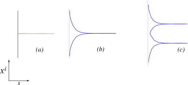
Figure 32: (a): A D3–brane (vertical) with a D1–brane ending on it (horizontal) is actually pulled (b) into a smooth interpolating shape. (c): Finitely separated D1–branes can only be described with non–commutative coordinates (see text)

We sketch this shape in figure 32(a). It is again our BIon–type solution, described before in section 4.6. The D3–brane smoothly interpolates between a pure D1–brane geometry far away and a spiked shape resembling D1–brane behaviour at the centre. A multi–centred solution is easy to construct as a superposition of harmonic solutions of the above type. Considering two of them, we see that in fact for any finite separation of the D1–branes (as measured far enough along the $s$–direction), by time we get to $s=1$, they will be arbitrarily close to each other (see 32(b)). We therefore cannot forget [179] about the off–diagonal parts of $\Phi^{m}$ corresponding to 1–1 strings stretching between the branes, and in fact we are forced to describe the geometry of the branes’ endpoints on the D3–brane using non–abelian $X^{m}$. This is another example of the “natural” occurrence of a non–commutativity arising in what we would have naively interpreted as ordinary spacetime coordinates.

We can see precisely what the boundary conditions must be, since we are simply asking that there be a pole in $\Phi^{i}(s)$ as $s\to\pm 1$:

$$\Phi^{i}(s)\to{\Sigma^{i}\over s\mp 1}\ ,$$ (380)

and placing this into (378), we see that the $k{\times}k$ residues must satisfy

$$[\Sigma^{i},\Sigma^{j}]=2{\rm i}\epsilon_{ijk}\Sigma^{k}\ .$$ (381)

In other words, they must form an $k$–dimensional representations of $SU(2)$! This representation must be irreducible, as we have seen. Otherwise it necessarily captures only the physics of $m$ infinitely separated clumps of D1–branes, for the case where the representation is reducible into $m$ smaller irreducible representations.

The problem we have constructed is that of monopoles [182, 183] of $SU(2)$ spontaneously broken to $U(1)$ via an adjoint Higgs field ${\bf H}$. [185] Ignoring the centre of mass of the D3–brane pair, this $SU(2)$ is on their world volume, and the separation is given by the vev, $H$ of the Higgs field. The first order “Bogomol’nyi” equations [51] are:

$$B_{i}\equiv{1\over 2}\epsilon_{ijk}F_{jk}=D_{i}{\bf H}\ ,\quad{\rm with}$$

$$\quad F_{ij}=\partial_{i}A_{j}-\partial_{j}A_{i}+[A_{i},A_{j}];\quad\quad D_{i}{\bf H}=\partial_{i}{\bf H}+[A_{i},{\bf H}]\ ,$$ (382)

with gauge invariance $(g({\bf x})\in SU(2))$:

$$A_{i}\to g^{-1}A_{i}g+g^{-1}\partial_{i}g;\quad{\bf H}\to g^{-1}{\bf H}g\ .$$ (383)

Static, finite energy monopole solutions satisfy

$$\|{\bf H}({\bf x})\|\equiv{1\over 2}{\rm Tr}\left[{\bf H}^{*}{\bf H}\right]\to H\ \quad{\rm as}\quad r\to\infty\ ,$$ (384)

where ${\bf x}=(x_{1},x_{2},x_{3})$, $r^{2}=x_{1}^{2}+x_{2}^{2}+x_{3}^{2}$, and $(2\pi\alpha^{\prime})H=L/2$, where $L$ is the separation of our D3–branes. The topological magnetic charge the monopoles carry comes from the fact that the vacuum manifold, which is $SU(2)/U(1)\sim S^{2}$, can wind an integer number of times around the $S^{2}$ at infinity, giving a stable solution whose charge is a fixed number times that integer.

In fact, we can construct the Higgs field and gauge field of monopole solution of the 3+1 dimensional gauge theory as follows. Given $k{\times}k$ Nahm data $(\Phi^{1},\Phi^{2},\Phi^{3})=2\pi\alpha^{\prime}(T_{1},T_{2},T_{3})$ solving the equation (378), there is an associated differential equation for a $2k$ component vector ${\bf v}(s)$:

$$\left\{{\bf 1}_{2N}{d\over ds}+\left({x^{a}\over 2}{\bf 1}_{k}+iT_{a}\right)\otimes\sigma^{a}\right\}{\bf v}=0\ .$$

There is a unique solution normalisable with respect to the inner product

$$<{\bf v}_{1},{\bf v}_{2}>=\int_{-1}^{1}{\bf v}^{\dagger}_{1}{\bf v}_{2}ds\ .$$

In fact, the space of normalisable solutions to the equation is four dimensional, or complex dimension 2. Picking an orthonormal basis ${\widehat{\bf v}}_{1},{\widehat{\bf v}}_{2}$, we construct the Higgs and gauge potential as:

$${\bf H} = i\left[\matrix{<s{\widehat{\bf v}}_{1},{\widehat{\bf v}}_{1}>&<s{\widehat{\bf v}}_{1},{\widehat{\bf v}}_{2}>\cr<s{\widehat{\bf v}}_{2},{\widehat{\bf v}}_{1}>&<s{\widehat{\bf v}}_{2},{\widehat{\bf v}}_{2}>}\right]\ ,$$

$$A_{i} = \left[\matrix{<{\widehat{\bf v}}_{1},\partial_{i}{\widehat{\bf v}}_{1}>&<{\widehat{\bf v}}_{1},\partial_{i}{\widehat{\bf v}}_{2}>\cr<{\widehat{\bf v}}_{2},\partial_{i}{\widehat{\bf v}}_{1}>&<{\widehat{\bf v}}_{2},\partial_{i}{\widehat{\bf v}}_{2}>}\right]\$$ (385)

The reader may notice a similarity between this means of extracting the gauge and Higgs fields, and the extraction (371)(372) of the instanton gauge fields in the previous section. This is not an accident. The Nahm construction is in fact a hyperKähler quotient which modifies the ADHM procedure. The fact that this arrangement of branes is T–dual to that of the $p$–$(p+4)$ system is the physical realisation of this fact, showing that the basic families of hypermultiplet fields upon which the construction is based (in the brane context) are present here too.

It is worth studying the case $k=1$, for orientation. In this case, the solutions $T_{i}$ are simply real constants $(2\pi\alpha^{\prime})\Phi_{i}=-ia_{i}/2$, having the meaning of the position of the monopole at ${\bf x}=(a_{1},a_{2},a_{3})$. Let us place it at the origin. Furthermore, as this situation is spherically symmetric, we can write ${\bf x}=(0,0,r)$. Writing components ${\bf v}=(w_{1},w_{2})$, we get a pair of simple differential equations with solution

$$w_{1}=c_{1}e^{-rs/2}\ ,\quad w_{2}=c_{2}e^{rs/2}\ .$$ (386)

An orthonormal basis is given by

$${\widehat{\bf v}}_{1}\ :\left(c_{1}=0\ ,c_{2}=\sqrt{{r\over e^{2r}-1}}\,\right)\,\,\ ;{\widehat{\bf v}}_{2}\ :\left(c_{2}=0\ ,c_{1}=\sqrt{{r\over 1-e^{-2r}}}\,\right)$$ (387)

and the Higgs field is simply:

$${\bf H}(r)={\hat{x}}_{i}\sigma_{i}{\varphi(r)\over r}\ ,\quad{\rm with}$$

$$\varphi(r)={r\over(e^{2r}-1)}\int_{-1}^{1}se^{rs}ds={r\coth r-1}\ .$$ (388)

(here ${\hat{x}}=(0,0,1)$) while the gauge field is:

$$A_{i}(r)=\epsilon_{ijk}\sigma_{j}{\hat{x}}_{k}{\sinh r-r\over r^{2}\sinh r}\ .$$ (389)

This is the standard one–monopole solution of Bogomol’nyi, Prasad and Sommerfield, the prototypical “BPS monopole”. [51, 52] We can insert the required dimensionful quantities:

$$\varphi(r)\to\varphi\left(Lr/4\pi\alpha^{\prime}\right)\ ,$$ (390)

to get the Higgs field:

$${\bf H}={\sigma_{3}\over r}\varphi\left({Lr\over 4\pi\alpha^{\prime}}\right)\longrightarrow{L\over 4\pi\alpha^{\prime}}\sigma_{3}\ ,\quad{\rm as}\quad r\to\infty\ ,$$ (391)

showing the asymptotic positions of the D3–branes to be $\pm L/2$, after multiplying by $2\pi\alpha^{\prime}$ to convert the Higgs field (which has dimensions of a gauge field) to a distance in $x^{6}$. A picture of the resulting shape [49, 195] of the D3–brane is shown in figure 33.

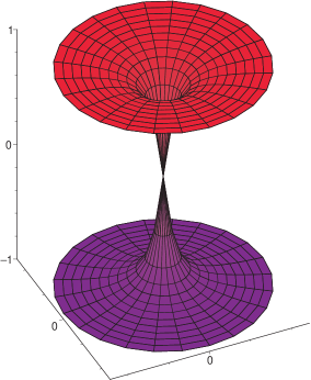
Figure 33: (a): A slice through part of two (horizontal) D3–branes with a (vertical) D1–brane acting as a single BPS monopole. This is made by plotting the exact BPS solution.

There is also a simple generalisation of the purely magnetic solution which makes a “dyon”, a monopole with an additional $n$ units of electric charge. It interpolates between the magnetic monopole behaviour we see here and the spike electric solution we found in section 4.6. It is amusing to note [40] that an evaluation of the mass of the solution gives the correct formula for the bound state mass of a D1–string bound to $n$ fundamental strings, as it should, since an electric point source is in fact the fundamental string.

10 D–Branes and Geometry II

10.1 The Geometry produced by D–Branes

By studying the supergravities arising in the low energy limit of the superstring theory, it was shown that there exist extended solutions resembling generalisations of charged black holes. The $p$ dimensional extended solution carries charges under the R–R form $C^{(p+1)}$. The extremal cases are BPS solutions, and they differ from Reissner–Nordstrom black holes in that their horizons at extremality have zero area . The BPS (extremal) solution is: [78, 79]

$$ds^{2} = Z_{p}^{-1/2}\eta_{\mu\nu}dx^{\mu}dx^{\nu}+Z_{p}^{1/2}dx^{i}dx^{i}\ ,$$

$$e^{2\Phi} = g^{2}_{s}{Z_{p}}^{(3-p)\over 2}\ ,$$

$$C_{(p+1)} = ({Z_{p}}^{-1}-1)g_{s}^{-1}dx^{0}\wedge\cdots\wedge dx^{p}\ ,$$ (392)

where $\mu=0,\ldots,p$, and $i=p+1,\ldots,9$, and the harmonic function $Z_{p}$ is

$$Z_{p}=1+{d_{p}(2\pi)^{p-2}g_{s}N\alpha^{\prime(7-p)/2}\over r^{7-p}}\ ;\quad d_{p}=2^{7-2p}\pi^{9-3p\over 2}\Gamma\left({7-p\over 2}\right)\ .$$ (393)

More complicated supergravity solutions preserving fewer supersymmetries (in the extremal case) can be made by combining these simple solutions in various ways, by intersecting them with each other, boosting them to finite momentum, and by wrapping, and/or warping them on compact geometries. This allows for the construction of finite area horizon solutions, corresponding to R–R charged Reissner–Nordstrom black holes, and generalisations thereof.

These solutions are R–R charged, but we have already established to all orders in string perturbation theory that D$p$–brane actually are the basic sources of these R–R fields. In fact, the solutions (392) are normalised such that they carry $N$ units of the basic D–brane charge $\mu_{p}$.

It is natural to suppose that there is a connection between these two families of objects: Perhaps the solution (392) is “made of D–branes” in the sense that it is actually the field due to $N$ D$p$–branes, all located at $r=0$. This is precisely how we are to make sense of this solution as a supergravity soliton solution. We must do so, since (except for $p=3$) the solution is actually singular at $r=0$, and so one might have simply discarded them as pathological, since solitons “ought to be smooth”, like the NS5–brane solution . However, string duality forces us to consider them, since smooth NS–NS solitons of various extended sizes (which can be made by wrapping or warping NS5–branes in an arbitrary compactification) are mapped [196] into these R–R solitons under it, generalizing what we have already seen in ten dimensions (see e.g. insert 11, (p.8.3)). With the understanding that there are D–branes “at their core”, which fits with the fact that they are R–R charged, they make sense of the whole spectrum of extended solitons in string theory.

Insert 13: The Type II NS5–brane In insert 11 (p.8.3) we deduced that there must be a solitonic brane, the NS5–brane, in type II string theory. We can deduce its supergravity fields by using the ten dimensional S–duality transformations to convert the case $p=5$ of equations (392), (393), to give: [55, 56] $\displaystyle ds^{2}$ $\displaystyle=$ $\displaystyle-dt^{2}+(dx^{1})^{2}+\cdots+(dx^{5})^{2}+{\tilde{Z}}_{5}\left(dr^{r}+r^{2}d\Omega_{3}^{2}\right)$ $\displaystyle e^{2\Phi}$ $\displaystyle=$ $\displaystyle g_{s}^{2}{\tilde{Z}}_{5}=g_{s}^{2}\left(1+{\alpha^{\prime}N\over r^{2}}\right)\ ,$ $\displaystyle B_{(6)}$ $\displaystyle=$ $\displaystyle({{\tilde{Z}}_{5}}^{-1}-1)g_{s}dx^{0}\wedge\cdots\wedge dx^{5}\ .$ (394) This solution has $N$ units of the basic magnetic charge of $B_{(2)}$, and is a point in $x^{6},x^{7},x^{8},x^{9}$. Here, $r^{2}$ is the radial coordinate, and $d\Omega_{3}^{2}$ is a metric on a round $S^{3}$. The tension of this BPS object was deduced in insert 11 (p.8.3) to be: $\tau^{\rm F}_{5}=(2\pi)^{-5}\alpha^{\prime-3}g_{s}^{-2}$. (Note that the same transformation will give a solution for the fields around a fundamental IIB string, by starting with the $p=1$ case of (392). [134, 135]) Recall also that we deduced the structure of this solution already using (a cavalier) T–duality to an ALE space in section 9.3. Here, we have used S–duality to the precise D–brane computations to see that our normalisations in those sections were correct.

Let us build up the logic of how they can be related to D–branes. Recall that the form of the action of the ten dimensional supergravity with NS–NS and R–R field strengths $H$ and $G$ respectively is, roughly:

$$S=\int d^{10}\!x\,\left(e^{-2\Phi}R-e^{-2\Phi}H^{2}-G^{2}\right)\ .$$ (395)

There is a balance between the dilaton dependence of the NS–NS and gravitational parts, and so the mass of a soliton solution [79] carrying NS–NS charge (like the NS5–brane) scales like the action: $T_{\rm NS}\sim e^{-2\Phi}\sim g_{s}^{-2}$. A R–R charged soliton has, on the other hand, a mass which goes like the geometric mean of the dilaton dependence of the R–R and gravitational parts: $T_{\rm R}\sim e^{-\Phi}\sim g_{s}^{-1}$. This is just the behaviour we saw for the tension of the D$p$–brane, computed in string perturbation theory, treating them as boundary conditions.

D$p$–branes have been treated so far largely as point–like (in their transverse dimensions) in an otherwise flat spacetime, and we were able to study an arbitrary number of them by placing the appropriate Chan–Paton factors into amplitudes. However, the solutions (392) have non–trivial spacetime curvature, and is only asymptotically flat. How are these two descriptions related?

The point is as follows: For every D$p$–brane which is added to a situation, another boundary is added to the problem, and so a typical string diagram has a factor $g_{s}N$ since every boundary brings in a factor $g_{s}$ and there is the trace over the $N$ Chan–Paton factors. So perturbation theory is good as long as $g_{s}N<1$. Notice that this is the regime where the supergravity solution (392) fails to be valid, since the curvatures are high. On the other hand, for $g_{s}N>1$, the supergravity solution has its curvature weakened, and can be considered as a workable solution. This regime is where the D$p$–brane perturbation theory, on the other hand, breaks down.

So we have a fruitful complementarity between the two descriptions. In particular, since we are only really good at string perturbation theory, i.e. $g_{s}<1$, for most computations, we can work with the supergravity solution with the interpretation that $N$ is very large, such that the curvatures are small. Alternatively, if one restricts oneself to studying only the BPS sector, then one can work with arbitrary $N$, and extrapolate results —-computed with the D–brane description for small $g_{s}$— to the large $g_{s}$ regime, (since there are often non–renormalisation theorems which apply) where they can be related to properties of the non–trivial curved solutions. This is the basis of the successful statistical enumeration of the entropy of black holes, for cases where the solutions (392) are used to construct R–R charged black holes. [202, 205] This exciting subject will be described in the notes of Amanda Peet. [203]

In summary, for a large enough number of coincident D–branes or for strong enough string coupling, one cannot consider them as points in flat space: they deform the spacetime according to the geometry given in eqn. (392). Given that D–branes are also described very well at low energy by gauge theories, this gives plenty of scope for finding a complementarity between descriptions of non–trivially curved geometry and of gauge theory. This is the basis of what might be called “gauge theory/geometry” correspondences. In some cases, when certain conditions are satisfied, there is a complete decoupling of the supergravity description from that of the gauge theory, signalling a complete duality between the two. This is the basis of the AdS/CFT correspondence, [199, 200] aspects of which are described in the lectures of Mike Duff and others.

10.2 Probing D–Branes’ Geometry with D–Branes: $p$ with D$p$

In the last section, we argued that the spacetime geometry given by equations (392) represents the spacetime fields produced by $N$ D$p$–branes. We noted that as a reliable (or “trustworthy”) solution to supergravity, the product $g_{s}N$ ought be be large enough that the curvatures are small. This corresponds to either having $N$ small and $g_{s}$ large, or vice–versa. Since we are good at studying situations with $g_{s}$ small, we can safely try to see if it makes sense to make $N$ large.

One way to imagine that this spacetime solution came about at weak coupling was that we built it by bringing in $N$ D$p$–branes, one by one, from infinity. If this is to be a sensible process, we must study whether it is really possible to do this. Imagine that we have been building the geometry for a while, bringing up one brane at a time from $r=\infty$ to $r=0$. Let us now imagine bringing the next brane up, in the background fields created by all the other $N$ branes. Since the branes share $p$ common directions where there is no structure to the background fields, we can ignore those directions and see that the problem reduces to the motion of a test particle in the transverse $9-p$ spatial directions. What is the mass of this particle, and what is the effective potential that it moves in?

This sort of question is answered by the still–developing toolbox which combines the fact that we have a gauge theory on D–branes with the fact that the probe brane is a heavy object which can examine many distance scales, and has seen many applications in our understanding of spacetime geometry in various situations. [86, 87, 88, 207, 208, 209]

We can derive the answers to all of the present questions by deriving an effective Lagrangian for the problem which results from the world–volume action of the brane. We can exploit the fact that we have spacetime Lorentz transformations and world–volume reparametrisations at our disposal to choose the work in the “static gauge”. In this gauge, we align the world–volume coordinates, $\xi^{a}$, of the brane with the spacetime coordinates such that:

$$\xi^{0}=x^{0}=t\ ;$$

$$\xi^{i}=x^{i}\ ;\quad i=1\cdots p\ ,$$

$$\xi^{m}=\xi^{m}(t)\ ;\quad m=p+1\cdots 9\ .$$ (396)

The Dirac–Born–Infeld part of the action (205) requires the insertion of the induced metric derived from the metric in question. In static gauge, it is easy to see that the induced metric becomes:

$$[G]_{ab}=\pmatrix{G_{00}+\sum_{mn}G_{mn}v_{m}v_{n}&0&0&\cdots&0\cr 0&G_{11}&0&\cdots&\vdots\cr\vdots&\vdots&\ddots&\vdots&\vdots\cr\vdots&\vdots&\vdots&\ddots&\vdots\cr 0&0&0&\cdots&G_{pp}}\ ,$$ (397)

where $v_{m}\equiv dx^{m}/d\xi^{0}={\dot{x}}^{m}$.

In our particular case of a simple diagonal metric, the determinant turns out as

$$\det[-G_{ab}]=Z_{p}^{-{(p+1)\over 2}}\left(1-Z_{p}\sum_{m=p+1}^{9}v_{m}^{2}\right)=Z_{p}^{-{(p+1)\over 2}}\left(1-Z_{p}v^{2}\right)\ .$$ (398)

The Wess–Zumino term representing the electric coupling of the brane is, in this gauge:

$$\mu_{p}\int C_{(p+1)} = \mu_{p}\int d^{p+1}\xi\,\,[C_{(p+1)}]_{\mu_{0}\mu_{1}...\mu_{p}}{\partial x^{\mu_{0}}\over\partial\xi^{a_{0}}}{\partial x^{\mu_{1}}\over\partial\xi^{a_{1}}}\cdots{\partial x^{\mu_{p}}\over\partial\xi^{a_{p}}}$$ (399)

$$= \mu_{p}V_{p}\int dt\left[Z_{p}^{-1}-1\right]g^{-1}\ ,$$

where $V_{p}=\int d^{p}\!x$, the spatial world–volume of the brane. Now, we are going to work in the approximation that we bring the branes slowly up the the main stack of branes so we keep the velocity $v$ small enough such that only terms up to quadratic order in $v$ are kept in our computation. We can therefore the expand the square root of our determinant, and putting it all together (not forgetting the crucial insertion of the background functional dependence of the dilaton from (392)) we get that the action is:

$$S = \mu_{p}V_{p}\int dt\left(-g_{s}^{-1}Z_{p}^{-1}+{1\over 2g_{s}}v^{2}+g_{s}^{-1}Z_{p}^{-1}-g_{s}^{-1}\right)$$ (400)

$$= \int dt{\cal L}=\int dt\left({1\over 2}m_{p}v^{2}-m_{p}\right)\ ,$$

which is just a Lagrangian for a free particle moving in a constant potential, (which we can set to zero) where $m_{p}=\tau_{p}V_{p}$ is the mass of the particle.

This result has a number of interesting interpretations. The first is simply that we have successfully demonstrated that our procedure of “building” our geometry (392) by successively bringing branes up from infinity to it, one at a time, makes sense: There is no non–trivial potential in the effective Lagrangian for this process, so there is no force required to do this; correspondingly there is no binding energy needed to make this system.

That there is no force is simply a restatement of the fact that these branes are BPS states, all of the same species. This manifests itself here as the fact that the R–R charge is equal to the tension (with a factor of $1/g_{s}$), saturating the BPS bound. It is this fact which ensured the cancellation between the $r$–dependent parts in (400) which would have otherwise resulted in a non–trivial potential $U(r)$. (Note that the cancellation that we saw only happens at order $v^{2}$ —the slow probe limit. Beyond that order, the BPS condition is violated, since it really only applies to statics.)

10.3 The Metric on Moduli Space

All of this has pertinent meaning from the point of view of field theory as well. Recall that there is a $U(N)$ $(p+1)$–dimensional gauge theory on a family of $N$ D$p$–branes. Recall furthermore that there is a sector of the theory which consists of a family of $(9-p)$ scalars, $\Phi^{m}$, in the adjoint. Geometrically, these are the collective coordinates for motions of the branes transverse to their world–volumes. Classical background values for the fields, (defining vacua about which we would then do perturbation theory) are equivalent to data about how the branes are distributed in this transverse space. Well, we have just confirmed that there is in fact a “moduli space” of inequivalent vacua of the theory corresponding to the fact that one can give a vacuum expectation value to a component of an $\Phi^{m}$ representing, representing a brane moving away from the clump of $N$ branes. That there is no potential translates into that fact that we can place the brane anywhere in this transverse clump, and it will stay there.

It is also worth noting that this metric on the moduli space is flat; treating the fields $\Phi^{m}$ as coordinates on the space ${\hbox{{\rm I}\kern-1.99997pt\hbox{\rm R}}}^{9-p}$, we see (from the fact that the velocity squared term in (400) appears as $v^{2}=\delta_{mn}v^{m}v^{n}$) that the metric seen by the probe is simply

$$ds^{2}\sim\delta_{mn}d\Phi^{m}d\Phi^{n}\ .$$ (401)

This flatness is a consequence of the high amount of supersymmetry (16 supercharges). For the case of D3–branes (whether or not they are in the AdS${}_{5}\times S^{5}$ limit), this result translates into the fact there that there is no running of the gauge coupling $g^{2}_{\rm YM}$ of the superconformal gauge theory on the brane. This is read off from the prefactor $g_{\rm YM}^{-2}=\tau_{3}(2\pi\alpha^{\prime})^{2}=(2\pi g_{s})^{-1}$ in the metric. The supersymmetry ensures that any corrections which could have been generated are zero. We shall now see a less trivial version, where we have a nontrivial metric in the case of eight supercharges.

10.4 Probing D–Branes’ Geometry with D–Branes: $p$ with D$(p-4)$.

Let us probe the geometry of the $p$–branes with a D$(p-4)$–brane. From our analysis of section 7, we know that this system is supersymmetric. Therefore, we expect that there should still be a trivial potential for the result of the probe computation, but there is not enough supersymmetry to force the metric to be flat. There are actually two sectors within which the probe brane can move transversely. Let us choose static gauge again, with the probe aligned so that its $p-4$ spatial directions $\xi^{1}-\xi^{p-4}$ are aligned with the directions $x^{1}-x^{p-4}$. Then there are four transverse directions within the $p$–brane background, labelled $x^{p-3}-x^{p}$, and which we can call $x_{\parallel}^{i}$ for short. There are $9-p$ remaining transverse directions which are transverse to the $p$–brane as well, labelled $x^{p+1}-x^{9}$ which we’ll abbreviate to $x_{\perp}^{m}$. The 6–2 case is tabulated as a visual guide:

	$x^{0}$	$x^{1}$	$x^{2}$	$x^{3}$	$x^{4}$	$x^{5}$	$x^{6}$	$x^{7}$	$x^{8}$	$x^{9}$
D2–brane	$-$	$-$	$-$	$\bullet$	$\bullet$	$\bullet$	$\bullet$	$\bullet$	$\bullet$	$\bullet$
6–brane	$-$	$-$	$-$	$-$	$-$	$-$	$-$	$\bullet$	$\bullet$	$\bullet$

Following the same lines of reasoning as above, the determinant which shall go into our Dirac–Born–Infeld Lagrangian is:

$$\det[-G_{ab}]=Z_{p}^{-{(p-3)\over 2}}\left(1-v_{\parallel}^{2}-Z_{p}v_{\perp}^{2}\right)\ ,$$ (402)

where the velocities come from the time ($\xi^{0}$) derivatives of $x_{\parallel}$ and $x_{\perp}$. This is nice, since in forming the action by multiplying by the exponentiated dilaton factor and expanding in small velocities, we get the Lagrangian

$${\cal L}={1\over 2}m_{p-4}\left(v_{\parallel}^{2}+Z_{p}v_{\perp}^{2}-2\right)\ ,$$ (403)

which again has a constant potential which we can discard, and pure kinetic terms. We see that there is a purely flat metric on the moduli space for the motion inside the four dimensions of the $p$–brane geometry, while there is a metric

$$ds^{2}=Z_{p}(r)\delta_{mn}dx^{m}dx^{n}\ ,$$ (404)

for the transverse motion. This is the Coulomb branch, in gauge theory terms, and the flat metric was on the Higgs branch. (In fact, the Higgs result does not display all of the richness of this system that we have seen. In addition to the flat metric geometry inside the brane that we see here, there is additional geometry describing the D$p$–D$(p-4)$ fields corresponding to the full instanton geometry. This “Yang–Mills geometry” comes from the fact that the D$(p-4)$–brane behaves as an instanton of the non–abelian gauge theory on the world–volume of the coincident D$p$–branes.)

Notice that for the fields we have studied, we obtained a trivial potential for free without having to appeal to a cancellation due to the coupling of the charge $\mu_{p-4}$ of the probe. This is good, since there is no electric source of this in the background for it to couple to. Instead, the form of the solution for the background makes it force–free automatically.

10.5 D2–branes and 6–branes: Kaluza–Klein Monopoles and M–Theory

Actually, when $p\geq 5$, something interesting happens. The electric source of $C_{(p+1)}$ potential in the background produces a magnetic source of $C_{(7-p)}$. The rank of this is low enough for there to be a chance for the D$(p-4)$–probe brane to couple to it even in the Abelian theory. For example, for $p=5$ there is a magnetic source of $C_{2}$ to which the D1–brane probe can couple. Meanwhile for $p=6$, there is a magnetic source of $C_{1}$. The D2–brane probes see this in an interesting way. Let us linger here to study this case a bit more closely. Since there is always a trivial $U(1)$ gauge field on the world volume of a D2–brane probe, corresponding to the centre of mass of the brane, we should include the coupling of the world–volume gauge potential $A_{a}$ (with field strength $F_{ab}$) to any of the fields coming from the background geometry.

In fact, as we saw before in section 6.2 there is a coupling

$$2\pi\alpha^{\prime}\mu_{2}\int_{M}C_{1}\wedge F\ ,$$ (405)

where $C_{1}=C_{\phi}d\phi$ is the magnetic potential produced by the 6–brane background geometry, which is easily computed to be: $C_{\phi}={-}(r_{6}/g_{s})\cos\theta$, where $r_{6}=gN\alpha^{\prime 1/2}/2$.

This extra degree of freedom on the world volume is equivalent to one scalar, since it comes from a gauge field in three dimensions. In our computations we may exchange $A_{a}$ for a scalar $s$, by Hodge duality in the (2+1)–dimensional world-volume. (This is of course a feature specific to the $p{=}2$ case.)

To get the coupling for this extra scalar correct, we should augment the probe computation. As we have seen, the Dirac–Born–Infeld action is modified by an extra term in the determinant:

$$-{\rm det}g_{ab}\to-{\rm det}(g_{ab}+2\pi\alpha^{\prime}F_{ab})\ .$$ (406)

We can [118, 141] introduce an auxiliary vector field $v_{a}$, replacing $2\pi\alpha^{\prime}F_{ab}$ by $e^{2\phi}\mu_{2}^{-2}v_{a}v_{b}$ in the Dirac action, and adding the term $2\pi\alpha^{\prime}\int_{M}F\wedge v$ overall. Treating $v_{a}$ as a Lagrange multiplier, the path integral over $v_{a}$ will give the action involving $F$ as before. Alternatively, we may treat $F_{ab}$ as a Lagrange multiplier, and integrating it out enforces

$$\epsilon^{abc}\partial_{b}(-\mu_{2}{\hat{C}}_{c}+v_{c})=0\ .$$ (407)

Here, ${\hat{C}}_{c}$ are the components of the pullback of $C_{1}$ to the probe’s world–volume. The solution to the constraint above is

$$-\mu_{2}{\hat{C}}_{a}+v_{a}=\partial_{a}s\ ,$$ (408)

where $s$ is our dual scalar. We may now replace $v_{a}$ by $\partial_{a}s+\mu_{2}{\hat{C}}_{a}$ in the action.

The static gauge computation picks out only ${\dot{s}}+\mu_{2}C_{\phi}{\dot{\phi}}$, and recomputing the determinant gives

$$\det=Z_{6}^{-{3\over 2}}\left(1-v_{\parallel}^{2}-Z_{6}v_{\perp}^{2}-{Z_{6}^{1\over 2}e^{2\Phi}\over\mu_{2}^{2}}\left[{\dot{s}}+\mu_{2}C_{\phi}{\dot{\phi}}\right]^{2}\right)\ .$$ (409)

Again, in the full Dirac–Born–Infeld action, the dilaton factor cancels the prefactor exactly, and including the factor of $-\mu_{2}$ and the trivial integral over the worldvolume directions to give a factor $V_{2}$, the resulting Lagrangian is

$${\cal L}={1\over 2}m_{2}(v_{\parallel}^{2}-2)+{1\over 2}V_{2}\left({\mu_{2}Z_{6}\over g}v_{\perp}^{2}+{g_{s}\over\mu_{2}Z_{6}}\left({\dot{s}}+\mu_{2}C_{\phi}{\dot{\phi}}\right)^{2}\right)\ ,$$ (410)

which is (after ignoring the constant potential) again a purely kinetic lagrangian for motion in eight directions. There is a non–trivial metric in the part transverse to both branes:

$$ds^{2}=V(r)\left({dr}^{2}+r^{2}{d\Omega}^{2}\right)+V(r)^{-1}\left({ds}+A_{\phi}d\phi\right)^{2}\ ,$$

with $$V(r)={\mu_{2}Z_{6}\over g_{s}}\quad\mbox{and}\quad A={\mu_{2}r_{6}\over g_{s}}\cos\theta d\phi\ ,$$ (411)

where ${d\Omega}^{2}={d\theta}^{2}+\sin^{2}\!\theta\,{d\phi}^{2}$. There is a number of fascinating interpretations of this result. In pure geometry, the most striking feature is that there are now eleven dimensions for our spacetime geometry. The D2–brane probe computation has uncovered, in a very natural way, an extra transverse dimension. This extra dimension is compact, since $s$ is periodic, which is inherited from the gauge invariance of the dual world–volume gauge field. The radius of the extra dimension is proportional to the string coupling, which is also interesting. This eleventh dimension is of course the M–direction we saw earlier. The D2–brane has revealed that the six–brane is a Kaluza–Klein monopole [138] of eleven dimensional supergravity on a circle, [126] which is constructed out of a Taub–NUT geometry (411). This fits very well with the fact that the D6 is the Hodge dual of the D0–brane, which we already saw is a Kaluza–Klein electric particle.

10.6 The Metric on Moduli Space

As before, the result also has a field theory interpretation. The $(2+1)$–dimensional $U(1)$ gauge theory (with eight supercharges) on the worldvolume of the D2–brane has $N_{f}=N$ extra hypermultiplets coming from light strings connecting it to the $N_{f}=N$ D6–branes. The $SU(N_{f})$ symmetry on the worldvolume of the D6–branes is a global “flavour” symmetry of the $U(1)$ gauge theory on the D2–brane. A hypermultiplet $\Psi$ has four components $\Psi_{i}$ corresponding to the 4 scalar degrees of freedom given by the four positions $\Psi^{i}\equiv(2\pi\alpha^{\prime})^{-1}x_{\parallel}^{i}$. The vector multiplet contains the vector $A_{a}$ and three scalars $\Phi^{m}\equiv(2\pi\alpha^{\prime})^{-1}x_{\perp}^{m}$. The Yang–Mills coupling is $g^{2}_{\rm YM}=g_{s}{\alpha^{\prime}}^{-1/2}$.

The branch of vacua of the theory with $\Psi\neq 0$ is called the “Higgs” branch of vacua while that with $\Phi\neq 0$ constitutes the “Coulomb” branch, since there is generically a $U(1)$ left unbroken. There is a non–trivial four dimensional metric on the Coulomb branch. This is made of the three $\Phi^{m}$, and the dual scalar of the $U(1)$’s photon. Let us focus on the quantities which survive in the low energy limit $\alpha^{\prime}\to 0$ and hold fixed any sensible gauge theory quantities which appear in our expressions. (Such procedures will be studied a lot in other lecture courses in this school). The metric which appears in (411) survives the limit as

$$ds^{2}=V(U)(dU^{2}+U^{2}d\Omega^{2}_{2})+V(U)^{-1}(d\sigma+A_{\phi}d\phi)^{2}$$

$$\mbox{where}\quad V(U)={1\over 4\pi^{2}g^{2}_{\rm YM}}\left(1+{g^{2}_{\rm YM}N_{f}\over 2U}\right)\ ;\quad A_{\phi}={N_{f}\over 8\pi^{2}}\cos\theta\ ,$$ (412)

where $U=r/\alpha^{\prime}$ has the dimensions of an energy scale in the gauge theory. Also, $\sigma=\alpha^{\prime}s$, and we will fix its period shortly.

In fact, the naive tree level metric on the moduli space is that on ${\hbox{{\rm I}\kern-1.99997pt\hbox{\rm R}}}^{3}\times S^{1}$, of form $ds^{2}=g^{-2}_{\rm YM}dx_{\perp}^{2}+g^{2}_{\rm YM}d\sigma^{2}$. Here, we have the tree level and one loop result: $V(U)$ has the interpretation as the sum of the tree level and one–loop correction to the gauge coupling of the 2+1 dimensional gauge theory. [209] Note the factor $N_{f}$ in the one loop correction. This multiplicity comes from the number of hypermultiplets which can run around the loop. Similarly, the cross term from the second part of the metric has the interpretation as a one–loop correction to the naive four dimensional topology, changing it to the (Hopf) fibred structure above.

Actually, the moduli space’s dimension had to be a multiple of four, as it generally has to be hyperKähler for $D{=}2+1$ supersymmetry with eight supercharges. [151] Our metric is indeed hyperKähler since it is the Taub–NUT metric: The hyperKähler condition on the metric in the form it is written is the by–now familiar equation: $\nabla\times{\bf A}={\nabla}V(U)$, which is satisfied.

In fact, we are not quite done yet. With some more care we can establish some important facts quite neatly. We have not been careful about the period of $\sigma$, the dual to the gauge field, which is not surprising given all of the factors of 2, $\pi$ and $\alpha^{\prime}$. To get it right is an important task, which will yield interesting physics. We can work it out in a number of ways, but the following is quite instructive. If we perform the rescaling $U=\rho/4g^{2}_{\rm YM}$ and $\psi=8\pi^{2}\sigma/N_{f}$, our metric is:

$$ds^{2}={g_{\rm YM}^{2}\over 64\pi^{2}}\,ds^{2}_{\rm TN}\ ,\quad{\rm where}$$

$$ds^{2}_{\rm TN}=\left(1+{2N_{f}\over\rho}\right)(d\rho^{2}+\rho^{2}d\Omega^{2}_{2})+4N^{2}\left(1+{2N_{f}\over\rho}\right)^{-1}(d\psi+\cos\theta d\phi)^{2}\ ,$$

(413)

which is a standard form for the Taub–NUT metric, with mass $N_{f}$, equal to the “nut parameter” for this self–dual case. [152] This metric is apparently singular at $\rho=0$, and in fact, for the correct choice of periodicity for $\psi$, this pointlike structure, called a “nut”, is removable, just like the case of the bolt singularity encountered for the Eguchi–Hanson space. (See insert 10, p.5.5.) Just for fun, insert 14 (p.10.6) carries out the analysis and finds that $\psi$ should have period $4\pi$, and so in fact the full $SU(2)$ isometry of the metric is preserved.

Insert 14: Removing the “Nut” Singularity from Taub–NUT The metric (413) will be singular at at the point $\rho=0$, for arbitrary periodicity of $\psi$. This will be a pointlike singularity which is called a “nut”, [65, 64] in contrast to the “bolt” we encountered for the Eguchi–Hanson space in insert 10 (p.5.5), which was an $S^{2}$. In this case, near $\rho=0$, if we make the space look like the origin of ${\hbox{{\rm I}\kern-1.99997pt\hbox{\rm R}}}^{4}$, we can make this pointlike structure into nothing but a coordinate singularity. Near $\rho=0$, we have: $$ds^{2}_{\rm TN}={2N_{f}\over\rho}\left(d\rho^{2}+\rho^{2}d\Omega^{2}_{2}+\rho^{2}(d\psi+\cos\theta d\phi)^{2}\right)\ ,$$ which is just the right metric for ${\hbox{{\rm I}\kern-1.99997pt\hbox{\rm R}}}^{4}$ if $\Delta\psi=4\pi$, the standard choice for the Euler coordinate. (This may have seemed somewhat heavy–handed for a result one would perhaps have guessed anyway, but it is worthwhile seeing it, in preparation for more complicated examples.)

What does this all have to do with gauge theory? Let us consider the case of $N_{f}=1$, which means one six brane. This is 2+1 dimensional $U(1)$ gauge theory with one hypermultiplet, a rather simple theory. We see that after restoring the physical scales to our parameterers, our original field $\sigma$ has period $1/2\pi$, and so we see that the dual to the photon is more sensibly defined as ${\widetilde{\sigma}}=4\pi^{2}\sigma$, which would have period $2\pi$, which is a more reasonable choice for a scalar dual to a photon. We shall use this choice later. With this choice, the metric on the Coulomb branch of moduli space is completely non–singular, as should be expected for such a simple theory.

Let us now return to arbitrary $N_{f}$. This means that we have $N_{f}$ hypermultiplets, but still a $U(1)$ 2+1 dimensional gauge theory with a global “flavour” symmetry of $SU(N_{f})$ coming from the six–branes. There is no reason for the addition of hypermultiplets to change the periodicity of our dual scalar and so we keep it fixed and accept the consequences when we return to physical coordinates $(U,{\widetilde{\sigma}})$: The metric on the Coulomb branch is singular at $U=0\,!$ This is so because insert 14 told us to give $\widetilde{\sigma}$ a periodicity of $2\pi N_{f}$, but we are keeping it as $2\pi$. So our metric in physical units has $\widetilde{\sigma}$ with period $2\pi$ appearing in the combination $(2d{\widetilde{\sigma}}+N_{f}\cos\theta d\phi)^{2}$. This means that the metric is no longer has an $SU(2)$ acting, since the round $S^{3}$ has been deformed into a “squashed” $S^{3}$, where the squashing is controlled by $N_{f}$. In fact, there is a deficit angle at the origin corresponding to an $A_{N_{f}-1}$ singularity.

How are we to make sense of this singularity? Well, happily, this all fits rather nicely with the fact that for $N_{f}>1$ there is an $SU(N_{f})$ gauge theory on the sixbranes, and so there is a Higgs branch, corresponding to the D2-brane becoming an $SU(N_{f})$ instanton! The singularity of the Coulomb branch is indeed a signal that we are at the origin of the Higgs branch, and it also fits that there is no singularity for $N_{f}=1$.

It is worthwhile carrying out this computation for the case of $N_{f}$ D6–branes in the presence of a negative orientifold 6–plane oriented in the same way. In that case we deduce from facts we learned before that the presence of the O6–plane gives global flavour group $SO(2N_{f})$ for $N_{f}$ D6–branes. The D2–brane however carries an $SU(2)$ gauge group. This is T–dual to the earlier statement made in section 9.4 about D9–branes in type I string theory carrying $SO(N_{f})$ groups while D5’s carry $USp(2M)$ groups. [108, 109]: The orientifold forces a pair of D2–branes to travel as one, with a $USp(2)=SU(2)$ group.

So the story now involves 2+1 dimensional $SU(2)$ gauge theory with $N_{f}$ hypermultiplets. The Coulomb branch for $N_{f}=0$ must be completely non–singular, since again there is no Higgs branch to join to. This fits with the fact that there are no D6–branes; just the O6–plane. The result for the metric on moduli space can be deduced from a study of the gauge theory (with the intuition gained from this stringy situation), and has been proven to be the Atiyah–Hitchin manifold. [206, 209, 224, 225] Some of this will be discussed in more detail in subsection 10.8. For the case of $N_{f}=1$, the result is also non–singular (there is again no Higgs branch for 1 D6–brane) and the result is a certain cover of the Atiyah–Hitchin manifold. [206, 224]. The case of general $N_{f}$ gives certain generalisations of the Atiyah–Hitchin manifold. [224, 226] The manifolds have $D_{N_{f}}$ singularities, consistent with the fact that there is a Higgs branch to connect to. Note also that a sringy interpretation of this result is that the strong coupling limit of these O6–planes is in fact M–theory on the Atiyah–Hitchin manifold, just like it is Taub–NUT for the D6–brane. 

10.7 When Supergravity Lies: Repulson Vs. Enhançon

Despite the successes we have achieved in the previous section with interpretation of supergravity solutions in terms of constituent D–branes, we should be careful, even in the case when we have supersymmetry to steer us away from potential pathologies. It is not always case that if someone presents us with a solution of supergravity with R–R charges that we should believe that it has an interpretation as being “made of D–branes”.

Consider again the case of eight supercharges. We studied brane configurations with this amount of supersymmetry by probing the geometry of $N$ (large) D$p$–branes with a single D$(p{-}4)$–brane. As described in previous sections, another simple way to achieve a geometry with eight supercharges from D–branes is to simply wrap branes on a manifold which already breaks half of the supersymmetry. The example mentioned was the four dimensional case of K3. In this case, we learned that if we wrap a D$(p{+}4)$–brane (say) on K3, we induce precisely one unit of negative D$p$–brane charge [92] supported on the unwrapped part of the worldvolume (see eqn.(300)). At large $N$ therefore, we might expect that there is a simple supergravity geometry which might be obtained by taking the solution for the D$(p+4)$–D$p$ system, and modifying the asymptotic charges to suit this situation. The resulting geometry naively should have the interpretation as that due to a large number $N$ of wrapped D$(p{+}4)$ branes:

$$ds^{2} = Z_{2}^{-1/2}Z_{6}^{-1/2}\eta_{\mu\nu}dx^{\mu}dx^{\nu}+Z_{2}^{1/2}Z_{6}^{1/2}dx^{i}dx^{i}+V^{1/2}Z_{2}^{1/2}Z_{6}^{-1/2}ds^{2}_{\rm K3}\ ,$$

$$e^{2\Phi} = g_{s}^{2}{Z_{p}}^{(3-p)/2}{Z_{p+4}}^{-(p+1)/2}\ ,$$

$$C_{\it(p+1)} = ({Z_{p}}^{-1}-1)g_{s}^{-1}dx^{0}\wedge dx^{1}\wedge\cdots\wedge dx^{p+1}$$

$$C_{\it(p+5)} = (Z_{p+4}^{-1}-1)g_{s}^{-1}dx^{0}\wedge dx^{1}\wedge\cdots\wedge dx^{p+5}\ .$$ (414)

Here, $\mu,\nu$ run over the $x^{0}-x^{p+1}$ directions, which are tangent to all the branes. Also $i$ runs over the directions transverse to all branes, $x^{p+2}-x^{5}$, and in the remaining directions, transverse to the induced brane but inside the large brane, $ds^{2}_{\rm K3}$ is the metric of a K3 surface of unit volume. $V$ is the volume of the K3 as measured at infinity, but the supergravity solution adjusts itself such that $V(r){=}VZ_{p}/Z_{p+4}$ is the measured volume of the K3 at radius $r$.

Let us focus on the case $p=2$, where we wrap D6–branes to get induced D2–branes. 

	$x^{0}$	$x^{1}$	$x^{2}$	$x^{3}$	$x^{4}$	$x^{5}$	$x^{6}$	$x^{7}$	$x^{8}$	$x^{9}$
D2	$-$	$-$	$-$	$\bullet$	$\bullet$	$\bullet$	$\bullet$	$\bullet$	$\bullet$	$\bullet$
D6	$-$	$-$	$-$	$\bullet$	$\bullet$	$\bullet$	$-$	$-$	$-$	$-$
K3	$-$	$-$	$-$	$-$	$-$	$-$	$\bullet$	$\bullet$	$\bullet$	$\bullet$

The harmonic functions are

$$Z_{2} = 1+\frac{r_{2}}{r}\ ,\quad r_{2}=-\frac{(2\pi)^{4}g_{s}N\alpha^{\prime 5/2}}{2V}\ ,$$

$$Z_{6} = 1+\frac{r_{6}}{r}\ ,\quad r_{6}=\frac{g_{s}N\alpha^{\prime 1/2}}{2}\ ,$$ (415)

normalised such that the D2– and D6–brane charges are $Q_{2}{=}{-}Q_{6}=-N$. Note that the smaller brane is delocalised in the K3 directions, as it should be, since the same is true of K3’s curvature.

We worked out the spectrum of type IIA supergravity theory compactified to six dimensions on K3 in subsection 5.5. The six dimensional supergravity theory has as an additional sector twenty–four $U(1)$’s in the R–R sector. Of these, twenty–two come from wrapping the ten dimensional two–form on the 19+3 two–cycles of K3. The remaining two are special $U(1)$’s for our purposes: One of them arises from wrapping IIA’s five–form entirely on K3, while the final one is simply the plain one–form already present in the uncompactified theory.

It is easy to see that there is something wrong with the geometry which we have just written down, representing the wrapping of the D6–branes on the K3. There is a naked singularity at $r=|r_{2}|$, known as the “repulson”, since it represents a repulsive gravitational potential, [214] as can be seen by scattering test particles in to small enough $r$. The curvature diverges there which is related to the fact that the volume of the K3 goes to zero there, and the geometry stops making sense. Let us look carefully to see if this is really the geometry produced by the branes. [211]

The object we have made should be a BPS membrane made of $N$ identical objects. These objects feel no force due to each other’s presence, and therefore the BPS formula for the total mass is simply (see eqn.(301))

$$\tau_{N}=\frac{N}{g_{s}}(\mu_{6}V-\mu_{2})$$ (416)

with $\mu_{6}=(2\pi)^{-6}\alpha^{\prime-7/2}$ and $\mu_{2}=(2\pi)^{-2}\alpha^{\prime-3/2}$. In fact, the BPS membrane is actually a monopole of one of the six dimensional $U(1)$’s. It is obvious which $U(1)$ this is; the diagonal combination of the two special ones we mentioned above. The D6–brane component is already a monopole of the IIA R–R one–form, and the D2 is a monopole of the five–form, which gets wrapped.

N.B.: As we shall see, the final combination is a non–singular BPS monopole, having been appropriately dressed [215] by the Higgs field associated to the volume of K3. Also, it maps [196] (under the strong/weak coupling duality of the type IIA string on K3 to the heterotic string on $T^{4}$) [125, 127, 72] to a bound state of a Kaluza–Klein monopole [138] and an H–monopole [217], made by wrapping the heterotic NS5–fivebrane. [211, 218, 219]

If we are to interpret our geometry as having been made by bringing together $N$ copies of our membrane, we ought to be able to carry out the procedure we described in the previous sections. We should see that the geometry as seen by the probe is potential–free and well–behaved, allowing us the interpretation of being able to bring the probe in from infinity.

The effective action for a D6–brane probe (wrapped on the K3) is:

$$S=-\int_{M}d^{3}\xi\,e^{-\Phi(r)}(\mu_{6}V(r)-\mu_{2})(-\det{g_{ab}})^{1/2}+\mu_{6}\int_{M\times\rm K3}\!C_{\it 7}-\mu_{2}\int_{M}C_{\it 3}\ .$$ (417)

Here $M$ is the projection of the world-volume onto the three non–compact dimensions. As discussed previously (see eqn.(303) and surrounding discussion), the first term is the Dirac–Born–Infeld action with the position dependence of the tension (416) taken into account; in particular, $V(r)=VZ_{2}(r)/Z_{6}(r)$. The second and third terms are the couplings of the probe charges $(\mu_{6},-\mu_{2})$ to the background R–R potentials, following from eqn (300), and surrounding discussion.

Having derived the action, the calculation proceeds very much as we outlined in the previous sections, with the result:

$${\cal L} = -\frac{\mu_{6}VZ_{2}-\mu_{2}Z_{6}}{Z_{6}Z_{2}g_{s}}+\frac{\mu_{6}V}{g_{s}}(Z_{6}^{-1}-1)-\frac{\mu_{2}}{g_{s}}(Z_{2}^{-1}-1)$$ (418)

$$\qquad\qquad\qquad\qquad{}+\frac{1}{2g_{s}}(\mu_{6}VZ_{2}-\mu_{2}Z_{6})v^{2}+O(v^{4})\ .$$

The position–dependent potential terms cancel as expected for a supersymmetric system, leaving the constant potential $(\mu_{6}V-\mu_{2})/g$ and a nontrivial metric on moduli space (the $O(v^{2})$ part) as expected with eight supersymmetries. The metric is proportional to

$$ds^{2}={1\over g_{s}}\left(\mu_{6}VZ_{2}-\mu_{2}Z_{6}\right)dx_{\perp}^{2}={\alpha^{\prime-3/2}\over(2\pi)^{2}g}\Biggl{(}\frac{V}{V_{*}}-1-\frac{g_{s}N\alpha^{\prime 1/2}}{r}\Biggr{)}(dr^{2}+r^{2}d\Omega^{2}_{2})\ .$$ (419)

We assume that $V>V_{*}\equiv(2\pi)^{4}\alpha^{\prime 2}$, so that the metric at infinity (and the membrane tension) are positive. However, as $r$ decreases the metric eventually becomes negative, and this occurs at a radius

$$r=\frac{2V}{{V}-V_{*}}|r_{2}|\equiv r_{\rm e}$$ (420)

which is greater than the radius $r_{\rm r}=|r_{2}|$ of the repulson singularity.

In fact, our BPS monopole is becoming massless as we approach the special radius. This should mean that the $U(1)$ under which it is charged is becoming enhanced to a non–abelian group. This is the case. There is a purely stringy phenomenon which lies outside the W–bosons are wrapped D4–branes, which enhance the $U(1)$ to an $SU(2)$. The masses of wrapped D4–branes is just like that of the membrane, and so becomes zero when the K3’s volume reaches the value $V_{*}{\equiv}(2\pi\sqrt{\alpha^{\prime}})^{4}$.

The point is that the repulson geometry represents supergravity’s best attempt to construct a solution with the correct asymptotic charges. In the solution, the volume of the K3 decreases from its asymptotic value $V$ as one approaches the core of the configuration. At the centre, the K3 radius is zero, and this is the singularity. This ignores rather interesting physics, however. At a finite distance from the putative singularity (where $V_{\rm K3}=0$), the volume of the K3 gets to $V{=}V_{*}$, so the stringy phenomena —including new massless fields— giving the enhanced $SU(2)$ should have played a role.  So the aspects of the supergravity solution near and inside the special radius, called the “enhançon radius”, should not be taken seriously at all, since it ignored this stringy physics.

To a first approximation, the supergravity solution should only be taken as physical down to the enhançon radius $r_{\rm e}$. That locus of points, a two–sphere $S^{2}$, is itself called an “enhançon”. [211]

Note also that the size of the monopole is inverse to the mass of the $W$ bosons, and so in fact by time our probe gets to the enhançon radius, it has smeared out considerably, and in fact merges into the geometry, forming a “shell” with the other monopoles at that radius. Since by this argument we cannot place sharp sources inside the enhançon radius, evidently, and so the geometry on the inside must be very different from that of the repulson. In fact, to a first approximation, it must simply be flat, forming a smooth junction with the outside geometry at $r=r_{\rm e}$.

In general, one expects the same sort of reasoning to apply for all $p$, and so the enhançon locus resulting from wrapping a D$(p+4)$–brane on K3 is $S^{4-p}\times R^{p+1}$, whose interior is $(5+1)$–dimensional. For even $p$ the theory in the interior has an $SU(2)$ gauge symmetry, while for odd $p$ there is the $A_{1}$ two–form gauge theory. The details of the smoothing will be very case dependent, and it should be interesting to work out those details.

One can also study $SO(2N)$, $SO(2N{+}1)$ and $USp(2N)$ gauge theories with eight supercharges in various dimensions using similar techniques, placing an orientifold O6–plane into the system parallel to the D6–branes. The enhançon then becomes an $\mathbf{RP}^{2}$. [220]

Note that the Lagrangian (418) depends only on three moduli space coordinates, $(x^{3},x^{4},x^{5})$, or $(r,\theta,\phi)$ in polar coordinates. As mentioned before, a (2+1) dimensional theory with eight supercharges, should have a moduli space metric which is hyperKähler. [151] So we need at least one extra modulus, $s$. A similar procedure to that used in section 10.5 can be used to introduce the gauge field’s correct couplings and dualize to introduce the scalar $s$. A crucial difference is that one must replace $2\pi\alpha^{\prime}F_{ab}$ by $e^{2\phi}(\mu_{6}V(r)-\mu_{2})^{-2}v_{a}v_{b}$ in the Dirac–Born–Infeld action, the extra complication being due to the $r$ dependent nature of the tension. The static gauge computation gives for the kinetic term:

$${\cal L}=F(r)\left({\dot{r}}^{2}+r^{2}{\dot{\Omega}}^{2}\right)+F(r)^{-1}\left({\dot{s}}/2-\mu_{2}C_{\phi}{\dot{\phi}}/2\right)^{2}\ ,$$ (421)

where

$$F(r)={Z_{6}\over 2g_{s}}\left(\mu_{6}V(r)-\mu_{2}\right)\ ,$$ (422)

and ${\dot{\Omega}}^{2}={\dot{\theta}}^{2}+\sin^{2}\!\theta\,{\dot{\phi}}^{2}.$

10.8 The Metric on Moduli Space

Again, there is gauge theory information to be extracted here. We have pure gauge $SU(N)$ theory with no hypermultiplets, and eight supercharges. We should be able to cleanly separate the gauge theory data from everything else by taking the decoupling limit $\alpha^{\prime}\to 0$ while holding the gauge theory coupling $g^{2}_{\rm YM}=g^{2}_{{\rm YM},p}V^{-1}=(2\pi)^{4}g_{s}\alpha^{\prime 3/2}V^{-1}$ and the energy scale $U=r/\alpha^{\prime}$ (proportional to $M_{W}$) fixed. In doing this, we get the metric:

$$ds^{2}=f(U)\left({\dot{U}}^{2}+U^{2}{d\Omega}^{2}\right)+f(U)^{-1}\left({d\sigma}-{N\over{4\pi^{2}}}A_{\phi}{d\phi}\right)^{2}\ ,$$

where $$f(U)={1\over 4\pi^{2}g^{2}_{\rm YM}}\left(1-{g^{2}_{\rm YM}N\over U}\right)\ ,$$ (423)

the $U(1)$ monopole potential is $A_{\phi}=\pm 1-\cos\theta,$ and $\sigma=s{\alpha^{\prime}}$, and the metric is meaningful only for $U{>}U_{\rm e}=\lambda$. This metric, which should be contrasted with equation (412), is the hyperKähler Taub–NUT metric, but this time with a negative mass. This metric is singular, but the full metric, obtained by instanton corrections to this one–loop result, should be smooth, as we will discuss. The details of this smoothing will teach us more about this $p=2$ case of the enhançon geometry and the interpolation between the exterior supergravity solution and the interior region, which is flat to leading order.

From the point of view of the monopole description, this manifold should be related to the metric on the moduli space of monopoles. This fits with the fact that the moduli space of the gauge theory and that of the monopole problem are known to be identified. [224, 221, 172] It is clearly a submanifold of the full $4N{-}4$ dimensional metric on the relative moduli space [186] of $N$ BPS monopoles which is known to be smooth. [194] For the problem of two monopoles, that moduli space manifold[222] is the Atiyah–Hitchin manifold, [206] while for general $N$ it is more complicated. This should remind the reader of our study in subsection 10.6. Recalling that this is also a study of $SU(N)$ gauge theory with no hypermultiplets, we know the result for $N=2$: The metric on the moduli space must be smooth, as there is no Higgs branch to connect to via the singularity. This is true for all $SU(N)$, and matches the monopole result. For $N=2$, we saw that the metric on the moduli space is actually the Atiyah–Hitchin manifold.

The structure of our particular four dimensional submanifold of the general moduli space is very similar to that of an Atiyah–Hitchin manifold, in fact! To see this, [223] change variables in our probe metric (423) by absorbing a factor of $\lambda/2=g^{2}_{\rm YM}N/2$ into the radial variable $U$, defining $\rho=2U/\lambda$. Further absorb $\psi=\sigma 8\pi^{2}/N$ and gauge transform to $A_{\phi}={-}\cos\theta$. Then we get:

$$ds^{2}={g^{2}_{\rm YM}N^{2}\over 32\pi^{2}}ds^{2}_{\rm TN-}\ ,\quad{\rm with}$$ (424)

$$ds^{2}_{\rm TN-}=\left(1-{2\over\rho}\right)\left({d\rho}^{2}+\rho^{2}{d\Omega}^{2}\right)+4\left(1-{2\over\rho}\right)^{-1}\left({d\psi}+\cos\theta{d\phi}\right)^{2}\ .$$

The latter is precisely the form of the Taub–NUT metric that one gets by expanding the Atiyah–Hitchin metric in large $\rho$ and neglecting exponential corrections.

Now for the same reasons as in subsection 10.6, the periodicity of $\sigma$ is $1/2\pi$, and we will use $\widetilde{\sigma}=4\pi^{2}\sigma$ as our $2\pi$ periodic scalar dual to the photon on the probe’s world–volume. Looking at the choices we made above, this implies that for the $SU(2)$ case, the coordinate $\psi$ has period $2\pi$ ! This is surprising (perhaps), but does not lead to a “nut” singularity (see insert 14, p.10.6) for the following reason: The nut would be at $\rho=0$, but there is a more dangerous singularity already at $\rho=2$. This new singularity is an artifact of a large $\rho$ expansion, however. There is a unique and completely non–singular manifold whose metric is as asymptotically close to $ds^{2}_{\rm TN-}$ up to exponential corrections, which is determined as follows:

In this case of $N=2$, there is an $SO(3)=SU(2)/{\hbox{{\rm Z}\kern-3.99994pt\hbox{\rm Z}}}_{2}$ isometry in the problem, and not the naive $SU(2)$ of the Taub–NUT space, since $\psi$ has period $2\pi$ and not $4\pi$. This isometry, smoothness, and the condition of hyperKählerity pick out uniquely the Atiyah–Hitchin manifold as the completion of the negative mass Taub–NUT and completes the story for the $SU(2)$ gauge theory moduli space problem. [224] The Atiyah–Hitchin manifold can be written in the following manifestly $SO(3)$ invariant manner: [206, 228]

$$ds^{2}_{\rm AH}=f^{2}d\rho^{2}+a^{2}\sigma_{1}^{2}+b^{2}\sigma_{2}^{2}+c^{2}\sigma_{3}^{2}\ ;$$

$${2bc\over f}{da\over d\rho} = (b-c)^{2}-a^{2}\ ,\mbox{ and cyclic perms.;}\quad\rho=2K\left(\sin{\beta\over 2}\right),$$ (425)

where the choice $f=-b/r$ can be made, the $\sigma_{i}$ are defined in (262), and $K(k)$ is the elliptic integral of the first kind:

$$K(k)=\int_{0}^{\pi\over 2}(1-k^{2}\sin^{2}\tau)^{1\over 2}d\tau\ .$$ (426)

Also, $k{=}\sin(\beta/2)$, the “modulus”, runs from $0$ to $1$, so $\pi\leq\rho\leq\infty$.

In fact, the solution for $a,b,c$ can be written out in terms of elliptic functions, but we shall not do that here. It is enough to note that when $\rho$ is large, the difference between this metric and $ds^{2}_{\rm TN-}$ is exponentially small in $\rho$. These exponential corrections for smaller $\rho$ remove the singularity: $\rho=2$ is just an artefact of the large $\rho$ metric in the above form (10.8).

The exponential corrections have the expected interpretation in the gauge theory as the instanton corrections. [225] Translating back to physical variables, we see that these corrections go as $\exp{(-U/g^{2}_{\rm YM})}$, which has the correct form of action for a gauge theory instanton. (We have just described a cover of the Atiyah–Hitchin manifold needed for the $SU(2)$ case. There is an additional identification to be discussed below.)

Can we learn anything from this for our case of general $N$, especially for large $N$, to teach us about the enhançon geometry? We have to be careful. Now, fixing our period of $\widetilde{\sigma}$ to be $2\pi$ as before, for general $N$ the reulting period of $\psi$ in the scaled variables is $\Delta\psi=4\pi/N$. Therefore our isometry is not $SO(3)$ but $SU(2)/{\hbox{{\rm Z}\kern-3.99994pt\hbox{\rm Z}}}_{N}$. (So the boundary at infinity is the squashed $S^{3}$, given by $S^{3}/{\hbox{{\rm Z}\kern-3.99994pt\hbox{\rm Z}}}_{N}$).

So the manifold we need is not quite the Atiyah–Hitchin manifold, but probably a close cousin; as the Atiyah–Hitchin manifold goes once around its $\psi$–circle, the manifold we need goes around $N/2$ times, and it is tempting to wonder if the manifold we seek is simply a smooth quotient of it. It would be interesting to find this manifold using requirements of uniqueness and smoothness. This manifod certainly exists, given the data that we have presented from the point of view of the gauge theory and the monopole physics.

Once we have found this manifold in scaled coordinates, we can then rescale everything back to the original physical variables. The rescaled exponential corrections should be the gauge theory instanton corrections which we expect, although for large $N$ they will be quite small, and the dominant geometry will be that of the negative mass Taub–NUT for a wide range of validity. [227]

Even without precise knowledge of the manifold we seek, we can learn much about our problem at large $N$: We are working on a very symmetric subspace of the full $4N-4$ dimensional relative moduli space of monopoles. The problem is of a large charge $N$ monopole being approached by a small charge 1 monopole probe. The Atiyah–Hitchin manifold ($N=2$) in standard variables used in (10.8) and (425) represents two charge 1 monopoles approaching one another from asymptotic large relative separation $\rho$. We can borrows some of the intuitive behaviour of the two monopole case, some interpretation: For the two charge 1 case, for small $\rho$ they begin to merge into a charge 2 monopole, and $\rho$ no longer has distinct meaning as a separation. The singularity at $\rho=2$ is never reached, as it is an artifact of the large $\rho$ expansion; instead $\rho=\pi$ is the case where the monopoles are coincident. It is a removable “bolt singularity” in the full Atiyah–Hitchin geometry, of exactly the type we saw in the case of the Eguchi–Hanson space in insert 10 (p.5.5).

Actually, we have described a trivial cover of the true Atiyah–Hitchin space. The two monopole problem has an obvious ${\hbox{{\rm Z}\kern-3.99994pt\hbox{\rm Z}}}_{2}$ symmetry coming from the fact that the monopoles are identical. Some field configurations described by the manifold as described up to now are overcounted, and so we must divide by this ${\hbox{{\rm Z}\kern-3.99994pt\hbox{\rm Z}}}_{2}$. The result is that the bolt is an $\mathbf{RP}^{2}$ instead of an $S^{2}$. We will not have such an identification for $N>2$.

Note that when we scale $\rho$ back to $U$, our coordinate $U$ (for large $U$) is truly a radial coordinate, as one extremely heavy monopole is at the centre, being probed by a charge 1 monopole. The generalisation of the Atiyah–Hitchin bolt then represents the place of closest approach of the probe, where it has smoothed out. This is the smoothed, “nonperturbative” enhançon locus.

11 D–Branes and Geometry III: Non–Commutativity

11.1 Open Strings with a Background B–Field

Let us return briefly to where we started out. Writing down the open string sigma model (in conformal gauge). Gathering together the various pieces from the early chapters, we have:

$$S={1\over 4\pi\alpha^{\prime}}\int_{\Sigma}\!d^{2}\!\sigma\left\{\left(g^{ab}G_{\mu\nu}(X)+\epsilon^{ab}B_{\mu\nu}(X)\right)\partial_{a}X^{\mu}\partial_{b}X^{\nu}\right\}+\int_{\partial\Sigma}\!d\tau A_{i}(X)\partial_{\tau}X^{i}\ .$$ (427)

We are going to focus on the case where we have some gauge field on the world volume of a D$p$–brane, which has world–volume coordinates $X^{i}$, for $i=0,\ldots,p$. Transverse coordinates are $X^{m}$, for $m=p+1,\ldots,9$. We shall also have, as usual a trivial background $G_{\mu\nu}=\eta_{\mu\nu};\,\,\Phi={\rm constant}$, and a constant background $B$ field. We can go and vary the action as we did before, and we will find that again our $X^{\mu}$’s satisfy the 2D wave equation, but we have slightly different boundary conditions at $\sigma=0,\pi$:

$$\partial_{\sigma}X^{i}+\partial_{\tau}X^{j}{\cal F}^{i}_{j}=0\ ,\quad X^{m}=x_{0}^{m}\ ,$$ (428)

where we have written the gauge invariant combination ${\cal F}=B+2\pi\alpha^{\prime}F$. The second part is the Dirichlet boundary condition, fixing $x_{0}^{m}$ as the positions of the D$p$–brane.

Before going any further, it is worth trying to interpret the modification to the Neumann boundary condition, in the light of what we already know. Let us choose two directions in which there are non trivial components of ${\cal F}$, let us say $X^{1}$ and $X^{2}$. So we have either non–zero $B_{12}$ or $F_{12}$, or both. Then writing out the condition, we have:

$$\partial_{\sigma}X^{1}+\partial_{\tau}X^{2}{\cal F}_{2}^{1}=0\ ;$$ (429)

$$\partial_{\sigma}X^{2}-\partial_{\tau}X^{1}{\cal F}_{2}^{1}=0\ ,$$ (430)

where we have used the fact that ${\cal F}$ is antisymmetric. Now, if we write ${\cal F}_{2}^{1}=\cot\theta$, then we have

$$\phantom{-}\cos\theta\partial_{\sigma}X^{1}+\sin\theta\partial_{\tau}X^{2}=0\ ;$$ (431)

$$-\sin\theta\partial_{\tau}X^{1}+\cos\theta\partial_{\sigma}X^{2}=0\ .$$ (432)

Now if we do a T–duality in the 2 direction, we exchange $\partial_{\sigma}$ and $\partial_{\tau}$’s action on $X^{2}$. Then we see that we can rotate by an angle $\theta$ in the 1–2 plane, to new axes $X^{\prime 1},X^{\prime 2}$ to get:

$$\partial_{\sigma}X^{\prime 1}=0\ ,\quad\partial_{\tau}X^{\prime 2}=0\ .$$ (433)

Now, $\partial_{\tau}X^{a}=0$ is not quite a Dirichlet condition in the direction $X^{a}$, but nearly. Instead of saying that there is a definite position $X^{a}=x_{0}^{a}$ that the string endpoint must be on, it is in fact a definite statement about the conjugate momentum. So we interpret this to mean that there is a Dirichlet condition, but that the associated position has not been specified, and so it can be anywhere in the direction $X^{a}$. So in fact, we have gone from a D2–brane filling the $X^{1},X^{2}$ directions to a D–brane lying along the $X^{\prime 1}$ direction (see figure 34(c)). Also, before rotation, we see that $\partial_{\sigma}X^{1}+\tan\theta\partial_{\sigma}X^{2}=0$ is simply specifying that there be a D1–brane lying at an angle $\theta$ in the 1–2 plane (See figure 34(b)). We saw this in previous sections, but it is worth repeating here. Furthermore, we can now look at the original mixed condition (430) and see that it is simply the specification of a D2–brane lying in the 1–2 plane, but the presence of ${\cal F}$ mixes in a D0–brane, but it is in fact completely delocalized in the plane. We know that this must be true, since it is only in that case that a D$p$–D$(p-2)$ combination can be supersymmetric, and it also must be so in order to be T–dual to a D1–brane.

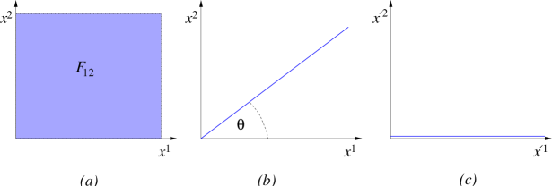
Figure 34: A brane in the 1–2 plane with a background field, (a), is dual to a tilted brane of one extended dimension fewer (b). It may then be rotated (c) to lie along a coordinate direction.

Further consequences come when we try to carry out the line of reasoning that we did in the early stages, in order to quantize the theory. [229] We can solve the 2D wave equation with the boundary conditions (430) to get the general solution:

$$X^{i}=x^{i}+2\alpha^{\prime}(p^{i}_{0}\tau-p^{j}_{0}{\cal F}^{i}_{j}\sigma)$$

$$\hskip 85.35826pt+(2\alpha^{\prime})^{1/2}\sum_{n\neq 0}{1\over n}e^{-in\tau}\left(i\alpha^{i}_{n}\cos n\sigma-\alpha^{j}_{n}{\cal F}^{i}_{j}\sin n\sigma\right)\ ,$$

$$X^{m}=x^{m}+Y^{m}\sigma+(2\alpha^{\prime})^{1/2}\sum_{n\neq 0}{1\over n}e^{-in\tau}\alpha^{i}_{n}\sin n\sigma\ ,$$ (434)

We have included the possibility that there is more than one D–brane, so that looking at $X^{m}$, it is clear that $Y^{m}$ is the separation between the brane that the ends of the string rest on. We will henceforth assume that both ends of the string lie on the same brane, and so $Y^{m}=0$. Also, in this case, we can rewrite our boundary term in the action as a bulk term $(1/2)\int_{\Sigma}d^{2}\!\sigma\,\epsilon^{\alpha\beta}F_{ij}\partial_{\alpha}X^{i}\partial_{\beta}X^{j}$, so that we see the appearance of $\cal F$ explicitly in the sigma model action.

It is interesting to follow the route further. The canonical momenta to $X^{\mu}$’s are

$$\Pi^{m}={1\over 2\pi\alpha^{\prime}}\partial_{\tau}X^{i}\ ;\qquad\Pi^{i}={1\over 2\pi\alpha^{\prime}}\left(\partial_{\tau}X^{i}+\partial_{\sigma}X^{j}{\cal F}_{j}^{i}\right)\ ,$$ (435)

from which we can compute the total conserved momentum:

$$P^{m}_{\rm tot}=0\ ;\qquad P^{i}_{\rm tot}=\int_{0}^{\pi}d\sigma\Pi^{i}(\tau,\sigma)=p^{j}_{0}M_{j}^{i}\ ,$$ (436)

where

$$M_{ij}=\eta_{ij}-{\cal F}_{i}^{k}{\cal F}_{kj}\ .$$ (437)

The Hamiltonian is then, using equations (59,60):

$$H={1\over 2}\left(M_{ij}p^{i}_{0}p^{j}_{0}+\sum_{n\neq 0}(M_{ij}\alpha_{n}^{i}\alpha_{-n}^{j}+\alpha^{m}_{n}\alpha^{m}_{-n})\right)\ ,$$ (438)

where we can see the non–trivial modification in the directions parallel to the brane, and nowhere else.

11.2 Non–Commutative Geometry and D–branes

Now the fun comes when we try to quantize. [229] The first thing to notice is that if we use the expression for the canonical momentum, and the boundary condition, we can derive that:

$$2\pi\alpha^{\prime}\Pi^{j}(\tau,0){\cal F}_{j}^{i}+\partial_{\sigma}X^{j}(\tau,0)M_{j}^{i}=0\ ,$$ (439)

so that, in particular

$$2\pi\alpha^{\prime}[\Pi^{j}(\tau,0),\Pi^{k}(\tau,\sigma)]{\cal F}_{j}^{i}=-[\partial_{\sigma}X^{j}(\tau,0),,\Pi^{k}(\tau,\sigma)]M_{j}^{i}\ .$$ (440)

But this is completely incompatible with our next step, [229] which is to try to impose the canonical commutation relations (67).

This is a case where our naive quantisation procedures break down, as happens in gauge theory when the gauge fixing condition is incompatible with the canonical approach. Like that situation, one has to use more careful methods, such as the constrained quantisation techniques of Dirac. We will not that here, but state the result, and refer the reader to the literature [229] for the details. The equal time commutators for the modes may be derived quite straightforwardly, and then used to infer the relations on the spacetime fields $X(\sigma,\tau),\Pi(\sigma,\tau)$:

$$[\Pi^{i}(\tau,\sigma),\Pi^{j}(\tau,\sigma^{\prime})]=0\ ,\quad[X^{i}(\tau,\sigma),X^{j}(\tau,\sigma^{\prime})]=0\ ;{\sigma\neq\sigma^{\prime}}$$

$$[X^{i}(\tau,\sigma),\Pi^{j}(\tau,\sigma^{\prime})]=i\eta^{ij}{1\over\pi}\left(1+\sum_{n\neq 0}\cos n\sigma\cos n\sigma^{\prime}\right)\ ;$$

$$[X^{i}(\tau,\sigma),X^{j}(\tau,\sigma^{\prime})]=e^{i\sigma}2i\pi\alpha^{\prime}(M^{-1}{\cal F})^{ij}\ ;\quad\sigma=\sigma^{\prime}=0,\pi$$ (441)

Now the remarkable thing is that the coordinates in the interior of the string (i.e., away from $\sigma=0,\pi$) satisfy the usual canonical commutation relations, but at the ends of the string, we see that there is actually some non–commutativity. For definiteness, let us look at our case of just the $X^{1},X^{2}$ plane again, and we see that, at the string endpoints, if we set only the spatial parts of ${\cal F}$ to be non–zero:

$$[X^{1},X^{2}]=2\pi i\alpha^{\prime}{{\cal F}\over 1+{\cal F}^{2}}\ ,$$ (442)

which is quite remarkable. Notice that we can have non–commutativity in time as well, if we turn on components of ${\cal F}$ in the time direction. Note that these “electric” components correspond to a boosted D–brane in the T–dual picture.

It is worth remarking that although this seems a bit strange, it is again just ordinary string theory looked at in a different way. Note that the rest of the studies we did in early sections go through. For example, the imposition of diffeomorphism invariance will still allow us to derive Virasoro generators:

$$L_{m}={1\over 2}\sum_{n=-\infty}^{\infty}\left(M_{ij}\alpha^{i}_{m-n}\alpha^{j}_{n}+\alpha_{m-n}\cdot\alpha_{n}\right)\ ,$$ (443)

where $\alpha_{l}\cdot\alpha_{k}\equiv\alpha^{m}_{l}\alpha_{k}^{m}$, the dot product in the transverse directions. After the standard normal ordering passing to the quantum story, it can be shown that they satisfy the usual Virasoro algebra. [229]

One last thing to notice is the fact that the mass spectrum may appear rather puzzling now. If we again follow the standard route, asking $L_{0}-1$ to vanish, we will get a formula

$$M_{ij}p_{0}^{i}p_{0}^{j}+\sum_{n=1}^{\infty}\left(M_{ij}\alpha^{i}_{m-n}\alpha^{j}_{n}+\alpha_{m-n}\cdot\alpha_{n}\right)-1=0\ .$$ (444)

The question is what to take as the definition of the mass. If we use the usual definition $M^{2}=-p^{i}p_{i}$, then we will have not only discrete contributions to the mass spectrum coming from the oscillators, but we will have continuous pats as well, coming from non–zero parts ${\cal F}$ in $M$. So we have a choice. We can either interpret this as a new feature of the string, or we can take the simpler approach and interpret all continuous parts as coming from the string having been streched. In other words, defining $M^{2}=-M_{ij}p^{i}p^{j}$ measures correctly the length of the string such that all other contributions to the mass spectrum are from the discrete oscillation energies. So to measure the length of our vector $p_{0}^{i}$, we used a natural metric associated to the open string in the presence of non–zero ${\cal F}$ which is different from $\eta_{ij}$, the metric that closed strings see. $M_{ij}$ is often called the “open string metric” in this context, and this is the reason why.

So we see that the spacetime coordinates on a D–brane in the presence of non–zero $\cal F$ are actually non–commutative. [230, 229] This makes a lot of sense, given our picture which we built up in the previous section: When ${\cal F}=0$, the endpoints of the string are instructed to simply end on the D$p$–brane, but for non–zero ${\cal F}$ there are D$(p-2)$–branes in the world–volume, but totally delocalised, since its presence is specified by a definite condition on momentum and not position. So the location of the string endpoints, in as much as they now make any definite sense, necessarily inherit an admixture of this delocalisation, taking on some of the characteristics of momentum, resulting in non–commutativity.

Many of the pieces of physics which we have investigated so far are worth revisiting in this light, and it might be worth keeping this picture in mind when the non–commutativity seems hard to accept. In particular, this means that the $\alpha^{\prime}\to 0$ limit of the open string sector should give Yang–Mills theory on non–commutative spacetimes. This has the amusing and sometimes confusing feature of endowing even Abelian Yang–Mills theory with non–commutative features. Gauge theories on non–commutative backgrounds is a subject of intense research at the time of writing.

11.3 Yang–Mills Geometry I: D–branes and the Fuzzy Sphere

In our many studies of the geometry seen by D–branes throughout these lectures, we kept using the idea that the spacetime coordinates transverse to the brane appear as scalar fields in a gauge theory on the brane’s world–volume. The vevs of these fields give the allowed positions of the brane in the spacetime, and so on. This allows for a remarkably rich dialogue between geometrical techniques and those of gauge theory.

When there are many branes, however, we know that the gauge theory becomes non–Abelian. This immediately leads to the idea [24] that this description forces us to consider non–commutative geometry in our spacetime, since the fields which we wish to interpret as coordinates have failed to commute.

This leads to non–commutative geometry of a naively different type from that which we encountered in the previous section, and there is potential for confusion. There really should not be. As we proceed with this process of blurring the distinction between descriptions of spacetime and other structures like string theory and gauge theory, the idea of non–commutative geometry as a natural language will arise again and again. One envisions it as something like the concept of the derivative: Differential calculus arises in many different situations, some of which are connected and some not. We do not search for deep connections for too long, but just see it as a tool and move on, knowing that being too philosophical about it is not necessarily very useful as a pursuit in itself; one expects that the same will be true of how we will regard the various situations where “geometry” has some degree of non–commutativity.

For the purposes of these notes, however, and because some readers might be trying to sort out the similarities and differences between these situations at a learning stage , I will call the non–commutative geometry in this section “Yang–Mills Geometry” and hope that this term is not too confusing.

The most familiar non–Abelian term which shows that there is something interesting to occur is of course the familiar scalar potential of the Yang–Mills theory. This of course appears in the Yang–Mills theory in the usual way, and can be thought of as resulting from the reduction of the ten dimensional Yang–Mills theory. It also arises as the leading part of the expansion of the $\det(Q^{i}_{j})$ term in the non–abelian Born–Infeld action, in the case when the brane is embedded in the trivial flat background $G_{\mu\nu}=\eta_{\mu\nu}$, as discussed in section 4.5:

$$V=\tau_{p}\,{\rm Tr}\sqrt{\det(Q^{i}{}_{j})}=N\tau_{p}+{\tau_{p}(2\pi\alpha^{\prime})^{2}\over 4}{\rm Tr}([\Phi^{i},\Phi^{j}]\,[\Phi^{j},\Phi^{i}])+\ldots\ ,$$ (445)

where $i=p+1,\ldots,9$. As we have discussed in a number of cases before, the simplest solution extremising $V$ is that the $\Phi^{i}$ all commute, in which case we can write them as diagonal matrices $\Phi^{i}=(2\pi\alpha^{\prime})^{-1}X^{i}$, where $X^{i}={\rm diag}(x^{i}_{1},x^{i}_{2},\ldots,x^{i}_{N})$. The interpretation is that $x^{i}_{n}$ is the coordinate of the $n$th D$p$–brane in the $X^{i}$ direction; we have $N$ parallel flat D$p$–branes, identically oriented, at arbitrary positions in a flat background, ${\hbox{{\rm I}\kern-1.99997pt\hbox{\rm R}}}^{9-p}$. The centre of mass of the D$p$–branes is at $x^{i}_{0}={\rm Tr}(X^{i})/N$. The potential is $N\tau_{p}$, which is simply the sum of all of the rest energies of the branes. We shall discard it in much of what follows.

When we look for situations with non–zero commutators, things become more complicated in interesting ways, giving us the possibility of new interesting extrema of the potential in the presence of non–trivial backgrounds. This is because the commutators appear in many parts of the worldvolume action, and in particular appear in couplings to the R–R fields, as we have seen in section 6.4. Furthermore, the background fields themselves depend upon the transverse coordinates $X^{i}$ even in the abelian case, and so will depend upon the full $\Phi^{i}$ in the non–abelian generalisation.

In general, this is all rather complicated, but we shall focus on one of the simpler cases as an illustration of the rich set of physical phenomena waiting to be uncovered. [44] Imagine that we have $N$ D$p$–branes in a constant background R–R $(p+4)$–form field strength $G_{(p+4)}=dC_{(p+3)}$, with non–trivial components:

$$G_{01...pijk}\equiv G_{tijk}=\matrix{-2f\varepsilon_{ijk}&i,j,k\in\{1,2,3\}}$$ (446)

(We have suppressed the indices $1...p$, as there is no structure there, and will continue to do so in what follows.) Let the D$p$–brane be pointlike in the directions $x^{i}$, $(i=1,2,3)$, and extended in $p$ other directions. None of these D$p$–branes in isolation is an electric source of this R–R field strength. Recall however, that there is a coupling of the D$p$–branes to the R–R $(p+3)$–form potential in the non–Abelian case, as shown in (298). We will assume a static configuration, choose static gauge

$$\zeta^{0}=t\ ,\quad\zeta^{\mu}=X^{\mu}\ ,\quad\mbox{ for }\mu=1,\ldots,p\ ,$$ (447)

and get (see (298)):

$$(2\pi\alpha^{\prime})\mu_{p}\int{\rm Tr}\,P\left[{\rm i}_{\Phi}{\rm i}_{\Phi}C\right]=$$

$$\quad=(2\pi\alpha^{\prime})\mu_{p}\int dt{\rm Tr}\left[\Phi^{j}\Phi^{i}\left(C_{ijt}(\Phi,t)+(2\pi\alpha^{\prime})C_{ijk}(\Phi,t)\,D_{t}\Phi^{k}\right)\right]\ .$$ (448)

We can now do a “non–Abelian Taylor expansion” [41, 232] of the background field about $\Phi^{i}$. Generally, this is defined as:

$$F(\Phi^{i})=\sum_{n=0}^{\infty}{(2\pi\alpha^{\prime})^{n}\over n!}\Phi^{i_{1}}\cdots\Phi^{i_{n}}\partial_{x^{i_{1}}}\cdots\partial_{x^{i_{1}}}F(x^{i})|_{x=0}\ .$$ (449)

and so:

$$C_{ijk}(\Phi,t)=C_{ijk}(t)+(2\pi\alpha^{\prime})\Phi^{k}\partial_{k}C_{ijk}(t)+{(2\pi\alpha^{\prime})^{2}\over 2}\Phi^{l}\Phi^{k}\partial_{l}\partial_{k}C_{ijk}(t)+\ldots$$ (450)

Now since $C_{ijt}(t)$ does not depend on $\Phi^{i}$, the quadratic term containing it vanishes, since it is antisymmetric in $(ij)$ and we are taking the trace. This leaves the cubic parts:

$$(2\pi\alpha^{\prime})^{2}\mu_{p}\int dt\,{\rm Tr}\left(\Phi^{j}\Phi^{i}\left[\Phi^{k}\partial_{k}C_{ijt}(t)+C_{ijk}(t)\,D_{t}\Phi^{k}\right]\right)$$

$$\qquad={1\over 3}(2\pi\alpha^{\prime})^{2}\mu_{p}\int dt\,{\rm Tr}\left(\Phi^{i}\Phi^{j}\Phi^{k}\right)G_{tijk}(t)\ ,$$ (451)

after an integration by parts. Note that the final expression only depends on the gauge invariant field strength, $G_{(p+4)}$. Since we have chosen it to be constant, this interaction (451) is the only term that need be considered, since of the higher order terms implicit in equation (450) will give rise to terms depending on derivatives of $G$.

Combining equation (451) with the part arising in the Dirac–Born-Infeld potential (445) yields our effective Lagrangian in the form $S=-\int dt{\cal L}$. This is a static configuration, so there are no kinetic terms and so ${\cal L}=-V(\Phi)$, with

$$V(\Phi)=-{(2\pi\alpha^{\prime})^{2}\tau_{p}\over 4}{\rm Tr}([\Phi^{i},\Phi^{j}]^{2})-{1\over 3}(2\pi\alpha^{\prime})^{2}\mu_{p}{\rm Tr}\left(\Phi^{i}\Phi^{j}\Phi^{k}\right)G_{tijk}(t)\ .$$ (452)

Let us substitute our choice of background field (446). The Euler–Lagrange equations $\delta V(\Phi)/\delta\Phi^{i}=0$ yield

$$[[\Phi^{i},\Phi^{j}],\Phi^{j}]+f\varepsilon_{ijk}[\Phi^{j},\Phi^{k}]=0\ .$$ (453)

Now of course, the situation of $N$ parallel static branes, $[\Phi^{i},\Phi^{j}]=0$ is still a solution, but there is a far more interesting one. [44] In fact, the non–zero commutator:

$$[\Phi^{i},\Phi^{j}]=f\,\varepsilon_{ijk}\Phi^{k}\ ,$$ (454)

is a solution. In other words we can choose

$$\Phi^{i}=-{\rm i}\,{f\over 2}\,\Sigma^{i}$$ (455)

where $\Sigma^{i}$ are any $N\times N$ matrix representation of the $SU(2)$ algebra

$$[\Sigma^{i},\Sigma^{j}]=2{\rm i}\,\epsilon_{ijk}\,\Sigma^{k}\ .$$ (456)

The $N\times N$ irreducible representation of $SU(2)$ has

$$(\Sigma^{i})^{2}={1\over 3}(N^{2}-1){\bf I}_{N\times N}\quad{\rm for}\ i=1,2,3.$$ (457)

where ${\bf I}_{N\times N}$ is the identity. Now the value of the potential (452) for this solution is

$$V_{\rm N}=-{\tau_{p}(2\pi\alpha^{\prime})^{2}f^{2}\over 6}\sum_{i=1}^{3}{\rm Tr}[(\Phi^{i})^{2}]=-{(2\pi)^{-p+2}\alpha^{\prime{3-p\over 2}}f^{4}\over 12g}N(N^{2}-1)\ .$$ (458)

So our noncommutative solution solution has lower energy than the commuting solution, which has $V=0$ (since we threw away the constant rest energy). This means that the configuration of separated D$p$–branes is unstable to collapse to the new configuration.

What is the geometry of this new configuration? Well, the $\Phi$’s are the transverse coordinates, and so we should try to understand their geometry, despite the fact that they do not commute. In fact, the choice (455) with the algebra (456) is that corresponding to the non–commutative or “fuzzy” two–sphere [231]. The radius of this sphere is given by

$$R_{N}^{2}=(2\pi\alpha^{\prime})^{2}{1\over N}\sum_{i=1}^{3}{\rm Tr}[(\Phi^{i})^{2}]=\pi^{2}\alpha^{\prime 2}f^{2}(N^{2}-1)\ ,$$ (459)

and so at large $N$: $R_{N}\simeq\pi\alpha^{\prime}fN$. The fuzzy sphere construction may be unfamiliar, and we refer the reader to the references for the details. [231] It suffices to say that as $N$ gets large, the approximation to a smooth sphere improves.

Note that the irreducible $N\times N$ representation is not the only solution. A reducible $N\times N$ representation can be made by direct product of $k$ smaller irreducible representations. Such a representation gives a ${\rm Tr}[(\Sigma^{i})^{2}]$ which is less than that for the irreducible representation (454), and therefore yields higher values for their corresponding potential. Therefore, these smaller representations representations, corresponding geometrically to smaller spheres, are unstable extrema of the potential which again would collapse into the single large sphere of radius $R_{N}$. It is amusing to note that we can adjust the solution representing an sphere of size $n$ by

$$\Phi^{i}=-{\rm i}{f\over 2}\,\Sigma_{n}^{i}+x^{i}\,{\bf I}_{n\times n}\ .$$ (460)

This has the interpretation of shifting the position of its centre of mass by $x^{i}$.

What we have constructed is a D$(p+2)$–brane with topology ${\hbox{{\rm I}\kern-1.99997pt\hbox{\rm R}}}^{p}\times S^{2}$. The ${\hbox{{\rm I}\kern-1.99997pt\hbox{\rm R}}}^{p}$ part is where the $N$ D$p$–branes are extended and the $S^{2}$ is the fuzzy sphere. There is no net D$(p+2)$–brane charge, as each infinitesimal element of the spherical brane which would act as a source of $C_{(p+3)}$ potential has an identical oppositely oriented (and hence oppositely charged) partner. There is therefore a “dipole” coupling due to the separation of these oppositely oriented surface elements. This type of construction is useful in matrix theory, where one can construct for example, spherical D2–brane backgrounds in terms of $N$ D0–branes variables. [232, 233, 234]

One way [49, 44] to confirm that we have made a spherical brane at large $N$, is to start with a spherical D$(p+2)$–brane, (topology ${\hbox{{\rm I}\kern-1.99997pt\hbox{\rm R}}}^{p}\times S^{2}$) and bind $N$ D$p$–branes to it, aligned along an ${\hbox{{\rm I}\kern-1.99997pt\hbox{\rm R}}}^{p}$. We can then place it in the background R–R field we first thought of and see if the system will find a static configuration keeping the topology ${\hbox{{\rm I}\kern-1.99997pt\hbox{\rm R}}}^{p}\times S^{2}$, with radius $R_{N}$. Failure to find a non–zero radius as a solution of this probe problem would be a sign that we have not interpreted our physics correctly.

Let us write the ten dimensional flat space metric with spherical polar coordinates on the part where the sphere is to be located ($x^{1},x^{2},x^{3}$):

$$ds^{2}=-dt^{2}+dr^{2}+r^{2}\left(d\theta^{2}+\sin^{2}\theta\,d\phi^{2}\right)+\sum_{i=4}^{9}(dx^{i})^{2}\ .$$ (461)

Our constant background fields in these coordinates is (again, suppresing the $1,\ldots,p$ indices):

$$G_{tr\theta\phi}=-2fr^{2}\,\sin\theta\ \quad\mbox{and so }\ C_{t\theta\phi}={2\over 3}fr^{3}\,\sin\theta\ .$$ (462)

As we have seen many times before, $N$ bound D$p$–branes in the D$(p+2)$–brane’s worldvolume corresponds to a flux due to the coupling:

$$(2\pi\alpha^{\prime})\mu_{p+2}\int_{{\cal M}^{3}}C_{(p+1)}\wedge F={\mu_{p}\over 2\pi}\int\!dt\,C_{(p+1)}\wedge F\ ,$$ (463)

where $C_{(p+1)}$ is the R–R potential to which the D$p$–branes couple, and is not to be confused with the $C_{(p+3)}$ we are using in our background, in (462). We need exactly $N$ D$p$–branes, so let us determine what $F$–flux we need to achieve this. If we work again in static gauge, with the D$(p+2)$–brane’s world–volume coordinates in the interesting directions being:

$$\zeta^{0}=t\ ,\quad\zeta^{1}=\theta\ ,\quad\zeta^{2}=\phi\ ,$$ (464)

then

$$F_{\theta\phi}={N\over 2}\sin\theta\ ,$$ (465)

is correctly normalised magnetic field to give our desired flux.

We now have our background, and our $N$ bound D$p$–branes, so let us seek a static solution of the form

$$r=R\quad\mbox{and $x^{i}=0$}\ ,\,\,\mbox{for $i=4,\ldots,9$}\ .$$ (466)

The world volume action for our D$(p+2)$–brane is:

$$S=-\tau_{p+2}\int\!dt\,d\theta\,d\phi\,e^{-\Phi}{\det{}^{1\over 2}(-G_{ab}+2\pi\alpha^{\prime}F_{ab})}+\mu_{p+2}\int C_{(p+3)}\ .$$ (467)

Assuming that we have the static trial solution (466), inserting the fields (462), a trivial dilaton, and the metric from (461), the potential energy is:

$$V(R) = -\int\!d\theta\,d\phi\,{\cal L}$$ (468)

$$= 4\pi\tau_{p+2}\left(\left[R^{4}+{(2\pi\alpha^{\prime})^{2}N^{2}\over 4}\right]^{{\textstyle{1\over 2}}}-{2f\over 3}R^{3}\right)$$

$$= {N}\tau_{p}+{2\tau_{p}\over(2\pi\alpha^{\prime})^{2}{N}}R^{4}-{4\tau_{p}\over 3(2\pi\alpha^{\prime})}fR^{3}+\ldots\ .$$

In the above we expanded the square root assuming that $2R^{2}/(2\pi\alpha^{\prime}){\rm N}<<1$, and kept the first two terms in the expansion. As usual we have substituted $\tau_{p}=4\pi^{2}\alpha^{\prime}\tau_{p+2}$.

The constant term in the potential energy corresponds to the rest energy of $N$ D$p$–branes, and we discard that as before in order to make our comparison. The case $V=0$ corresponds to $R=0$, the solution representing flat D$p$–branes. Happily, there is another extremum:

$$R=R_{N}=\pi\alpha^{\prime}fN\quad{\rm with}\ V=-{(2\pi)^{-p+2}\alpha^{\prime{3-p\over 2}}f^{4}\over 12g_{s}}N^{3}\ .$$

To leading order in $1/N$, we see that we have recovered the radius (and potential energy) of the non–commutative sphere configuration which we found in equations (459) and (458).

As noted before, this spherical D$(p+2)$–brane configuration carries no net D$(p+2)$–brane charge, since each surface element of it has an antipodal part of opposite orientation and hence opposite charge. However, as the sphere is at a finite radius, there is a finite dipole coupling.

This is the D–brane analogue [44] of the dielectric effect in electromagnetism. If we place D$p$–branes in a background R–R field under which the D$p$–branes would normally be regarded as neutral, the external field “polarises” the D$p$–branes, making them puff out into a (higher dimensional) non–commutative world–volume geometry. Just as in electromagnetism, where an external field may induce a separation of charges in neutral materials, the D–branes respond through the production of electric dipole and possibly higher multipole couplings via the non–zero commutators of the world–volume scalars.

There is clearly a rich set of physical phenomena to be uncovered by considering non–commuting $\Phi$’s. Already there have been applications of this mechanism to the understanding of a number of systems, such as large $N$ gauge theory in the AdS/CFT correspondence. [236]

11.4 Yang–Mills Geometry II: Enhançons and Monopoles

As a final example of how “Yang–Mills” non–commutative geometry naturally arises, let us return to our study of the enhançon. There, we we probed the metric geometry of the $N$ D6 branes wrapped on K3, and found that the true geometry deviates from the naive geometry due to stringy effects invisible in supergravity. The deviations were consistent with the fact that the probe was actually a magnetic monopole of one of the $U(1)$’s of the six dimensional theory. At a special radius the $U(1)$ gets enhanced to $SU(2)$ and the monopole becomes massless. Crucially for our concerns here, the monopole also stops being pointlike, and begins to spread out.

If this is the case, then in the light of what we have learned, it should mean that the world–volume fields describing the transverse coordinates of the wrapped brane must have become non–commutative describing their smearing. Does there exist a useful description of this? Luckily, the answer to this is in the affirmative.

Recall that the wrapped D6–brane is actually a charge $N$ monopole of the spontaneously broken $SU(2)$ six dimensional gauge theory. There is already a description of the $N$ monopole solution in terms of $N\times N$ matrices of $SU(N)$. It is Nahm’s equations shown in equation (378). While we derived them for D1–branes stretched between D3–branes, the monopole aspect of the description is essentially the same. This can also be seen by the following chain of dualities: K3 shrinking to volume $V_{*}=(2\pi)^{4}\alpha^{\prime 2}$ is in fact T–dual to K3 at a collapsed $A_{1}$ singularity, where the B–flux is going to zero. The wrapped D6–branes become D4–branes wrapping the collapsed singularity [211] We are on the Coulomb branch where the resulting D2–branes have split into two fractional ones, each carrying an $SU(N)$. We are focusing on one of them, and so send the other one off to infinity. 

As we learned in subsection 9.3 this situation is in turn T–dual to fractional D3–branes stretched between NS5–branes, where we focus on just one segment, and send the other to infinity. A D3–brane stretched between NS5–branes in this way is a monopole of the $U(1)$ gauge theory on the fivebrane worldvolume. The B–field is the distance between the NS5–branes, and when it goes to zero they coincide and there is an enhanced $SU(2)$.

	$x^{0}$	$x^{1}$	$x^{2}$	$x^{3}$	$x^{4}$	$x^{5}$	$x^{6}$	$x^{7}$	$x^{8}$	$x^{9}$
D3	$-$	$-$	$-$	$\bullet$	$\bullet$	$\bullet$	$|-|$	$\bullet$	$\bullet$	$\bullet$
NS5	$-$	$-$	$-$	$-$	$-$	$-$	$\bullet$	$\bullet$	$\bullet$	$\bullet$

The enhançon phenomenon, where the $SU(2)$ is enhanced on a sphere in spacetime, is the result of the bending of the NS5–branes as the D3–branes pull on them. [211] (This is shown for all $p$ in figure 35. The case we are discussing here is $p=2$.)

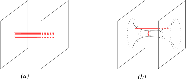
Figure 35: $N$ D$(p+1)$–branes ending on NS5–branes: (a) The naive picture (b) The resulting bending of the NS5–branes cannot be neglected for large $g_{s}N$. The separated brane is the probe which becomes massless at the enhançon locus, an $S^{4-p}$ (a circle in the figure).

The $N$ D3–brane configuration has a description as an $N$–monopole in the NS5–brane worldvolume. The earlier appearance of the Nahm equations is therefore manifestly connected to the geometry of the arrangement in the figure. The distance between the NS5–branes is the Higgs vev.

N.B.: Using type IIB’s S–duality converts the NS5–branes to D5–branes, and leaves alone the D3–branes stretched between them. A T–duality in the two spatial directions common to all the D–branes will complete the journey to the system of the D1’s stretched between two D3’s.

The $N{\times}N$ fields $\Phi^{i}(s)$ which appear in Nahm’s equations (378) represent the transverse coordinates of the $N$ D3–branes, in directions $x^{3},x^{4},x^{5}$. However as we have already seen in the discussion of monopoles, they are necessarily non–commutative. At the ends of the interval they must form an irreducible $N$ dimensional representation of $SU(2)$. These are precisely the same data which built the fuzzy sphere in our previous example. [223]

It is clear from this that at large $N$, a cross section of the $N$–monopole depicted in figure 35 has a description as a fuzzy sphere. The enhançon, which is the surface of the central slice is therefore describable as a fuzzy sphere. (Other points in the full monopole moduli space will describe other fuzzy geometries.) As $N$ is large, this is spherical to a good approximation and matches onto the spherically symmetric supergravity geometry in (414).

Unfortunately, it is has not been possible to write down the spacetime gauge and Higgs fields for multi–monopole solutions, as it is clearly interesting to study them more in detail. The construction of the full solutions are rather implicit, using algrebraic, and other methods from scattering theory, etc. [187, 188, 189, 190, 191, 192, 193] It would be an interesting problem to study how those fields match onto the asymptotic spherically symmetric supergravity fields of the solution (414). The explicit solutions, if we had them, might tell us much about both the supergravity geometry and possibly the large $N$ gauge theory on the wrapped brane, perhaps deepening the already known correspondence between their moduli spaces, [224, 221, 172] as discussed in detail in section 10.8.

Is short, we see that the intuitive reason for non–commutativity in this and the previous subsection is simply the fact that branes, for one reason or another, cease to be pointlike and/or lose their identity among other branes, becoming “smeared” or “dissolved”. This process is controlled/described by non–commutativity in some choice of variables. Since the endpoints of the strings are meant to be located on the branes, the smearing results in a natural departure from commutativity for our spacetime coordinates if we insist on continuing to use the variables we used when the branes were pointlike.

12 Closing Remarks

I think that it is high time that I stopped, since these notes have begun to become unwieldy. While there has been some repetition of ideas and phrases in various places, it was worth doing since it is by understanding something in as many different ways as one can that one can move beyond it. Particularly repetitious were the continued T–duality demonstrations (most things seemed to be explained by tilting a brane!), for which I make no apology.

As a means of making up for the rather large size of the notes, I collect towards the end a page or two of some of the most useful formulae that people like to have to hand (and their number in the text so that you can find where they are discussed/derived). Also, I have listed the titles and locations of the various inserts, which I hope are useful.

—cvj

Appendix A Collection of (Hopefully) Useful Formulae

Charges and tensions

• The fundamental string tension:

  $$\tau^{\rm F}_{1}\equiv T=(2\pi\alpha^{\prime})^{-1}=\nu_{1}\ .$$

  ($\nu_{1}$ is its $B_{(2)}$–charge.)

• The tension and charge of a D$p$–brane in superstring theory (272):

  $$\tau_{p}=\mu_{p}g_{s}^{-1}=(2\pi)^{-p}{\alpha^{\prime}}^{-(p+1)/2}g_{s}^{-1}\ .$$

• A recursion relation (181):

  $$\tau_{p}=\tau_{p^{\prime}}(2\pi\sqrt{\alpha^{\prime}})^{p^{\prime}-p}\ .$$

• The tension of the NS5–brane (see insert 11 (p.8.3))

  $$\tau^{\rm F}_{5}=(2\pi)^{-5}\alpha^{\prime{-3}}g_{s}^{-2}\ .$$

• The Yang Mills coupling for the field theory on a brane (274):

  $$g^{2}_{{\rm YM},p}=\tau_{p}^{-1}(2\pi\alpha^{\prime})^{-2}=(2\pi)^{p-2}\alpha^{\prime(p-3)/2}\ .$$

• Orientifold charge and tension (278):

  $$\mu^{\prime}_{p}=\mp 2^{p-5}\mu_{p},\qquad\tau^{\prime}_{p}=\mp 2^{p-5}\tau_{p}\ .$$

  (The minus sign is correlated with $SO$ and the plus with $USp$.)

• The product of the dual D–branes’ tensions

  $$\tau_{p}\tau_{6-p}=2\pi(2\pi)^{-7}\alpha^{\prime-4}g_{s}^{-2}={2\pi\over 2\kappa^{2}}$$

  is the minimum allowed by the quantum theory, with the following formula:

• The 10 dimensional Newton’s constant (252)

  $$2\kappa^{2}\equiv 2\kappa_{0}^{2}g_{s}^{2}=(16\pi G_{N})=(2\pi)^{-1}(4\pi^{2}\alpha^{\prime})^{4}g_{s}^{2}=(2\pi)^{7}\alpha^{\prime 4}g_{s}^{2}\ .$$

• The tensions of the M2– and M5–branes of 11 dimensional supergravity:

  $$\tau^{\rm M}_{2}=(2\pi)^{-2}\ell_{p}^{-3}\ ;\qquad\tau^{\rm M}_{5}=(2\pi)^{-5}\ell_{p}^{-6}\ ,$$

  can be deduced from the fact that the low energy type IIA string theory is 11 dimensional supergravity at strong coupling, that the D2–branes and NS5–branes directly lift to become the M–branes, and the following:

• The 11 dimensional Planck length $\ell_{p}$ (336):

  $$\ell_{p}=g_{s}^{1/3}\sqrt{\alpha^{\prime}}.$$

• The product of the M–branes’ tensions

  $$\tau^{\rm M}_{2}\tau^{\rm M}_{5}=2\pi(2\pi)^{-8}\ell_{p}^{-9}={2\pi\over 2\kappa_{11}^{2}}$$

  is the minimum allowed by the quantum theory, with:

• The 11 dimensional Newton constant (336):

  $$16\pi G_{N}^{11}=2\kappa_{11}^{2}\ ;\qquad\kappa_{11}^{2}=2^{7}\pi^{8}\ell_{p}^{9}.$$

• D–brane action (205), (268):

  $$S_{p}=-T_{p}\int d^{p+1}\xi\,e^{-\Phi}\det\!^{1/2}(G_{ab}+B_{ab}+2\pi\alpha^{\prime}F_{ab})+\mu_{p}\int_{{\cal M}_{p+1}}C_{(p+1)}\ .$$

• Some curvature couplings (291):

  $$\mu_{p}\int_{{\cal M}_{p+1}}\sum_{i}C_{(i)}\left[e^{2\pi\alpha^{\prime}F+B}\right]\sqrt{{\hat{\cal A}}(4\pi^{2}\alpha^{\prime}R)}\ .$$

  where the “A–roof” or “Dirac” genus has its square root defined as:

  $$\sqrt{{\hat{\cal A}}(R)}=1-{p_{1}(R)\over 48}+p_{1}^{2}(R){7\over 11520}-{p_{2}(R)\over 2880}+\cdots$$

  The $p_{i}(R)$’s are the $i$th Pontryagin class. For example,

  $$p_{1}(R)=-{1\over 8\pi^{2}}{\rm Tr}R\wedge R\ .$$

Bosonic Effective Actions

• The Dirac–Born–Infeld–Wess–Zumino Action (205)

  $$S=-\tau_{p}\int d^{p+1}X\,\det\!^{1/2}(\eta_{ab}+\partial_{a}X^{m}\partial_{b}X_{m}+2\pi\alpha^{\prime}F_{ab})+\mu_{p}\int C_{(p+1)}\ ,$$

• Type IIA string frame effective actions (249),(250)

  $$S_{\rm IIA}={1\over 2\kappa_{0}^{2}}\int\!d^{10}\!x(-G)^{1/2}\left\{e^{-2\Phi}\left[R+4(\nabla\phi)^{2}-{1\over 12}(H^{(3)})^{2}\right]\right.$$

  $$\qquad\quad\left.-{1\over 4}(G^{(2)})^{2}-{1\over 48}(G^{(4)})^{2}\right\}-{1\over 4\kappa_{0}^{2}}\int B^{(2)}dC^{(3)}dC^{(3)}\ .$$

  $H^{(3)}=dB^{(2)}$, $G^{(2)}=dC^{(1)}$ and $G^{(4)}=dC^{(3)}+H^{(3)}\wedge C^{(1)}$.

  $$S_{\rm IIB}={1\over 2\kappa_{0}^{2}}\int\!d^{10}\!x(-G)^{1/2}\left\{e^{-2\phi}\left[R+4(\nabla\phi)^{2}-{1\over 12}(H^{(3)})^{2}\right]\right.$$

  $$\left.\qquad\qquad\qquad-{1\over 12}(G^{(3)}+C^{(0)}H^{(3)})^{2}-{1\over 2}(dC^{(0)})^{2}-{1\over 480}(G^{(5)})^{2}\right\}$$

  $$\qquad\qquad\qquad+{1\over 4\kappa_{0}^{2}}\int\left(C^{(4)}+{1\over 2}B^{(2)}\,C^{(2)}\right)\,G^{(3)}\,H^{(3)}\ .$$

  $G^{(3)}=dC^{(2)}$ and $G^{(5)}=dC^{(4)}+H^{(3)}C^{(2)}$, $C^{(0)}$. Impose self–duality of $C^{(4)}$ via $F^{(5)}=\,^{*}\!F^{(5)}$ by hand in the equations of motion.

• Use

  $${\widetilde{G}}_{\mu\nu}=e^{-\Phi/2}G_{\mu\nu}\ ,$$

  to go to the Einstein frame.

• Type I Bosonic Action (253)

  $$S_{\rm I}={1\over 2\kappa_{0}^{2}}\int\!d^{10}\!x(-G)^{1/2}\Biggl{\{}e^{-2\Phi}\left[R+4(\nabla\phi)^{2}\right]$$

  $$\hskip 113.81102pt-{1\over 12}({\widetilde{G}}^{(3)})^{2}-{\alpha^{\prime}\over 8}e^{-\Phi}{\rm Tr}(F^{(2)})^{2}\Biggr{\}}\ .$$

  Here

  $${\widetilde{G}}^{(3)}=dC^{(2)}-{\alpha^{\prime}\over 4}\left[\omega_{\rm 3Y}(A)-\omega_{\rm 3L}(\Omega)\right]\ ,$$

• Heterotic actions (257)

  $$S_{\rm H}={1\over 2\kappa_{0}^{2}}\int\!d^{10}\!x(-G)^{1/2}e^{-2\Phi}\Biggl{\{}R+4(\nabla\phi)^{2}-{1\over 12}({\widetilde{H}}^{(3)})^{2}-{\alpha^{\prime}\over 8}{\rm Tr}(F^{(2)})^{2}\Biggr{\}}\ ,$$

  $${\widetilde{H}}^{(3)}=dB^{(2)}-{\alpha^{\prime}\over 4}\left[\omega_{\rm 3Y}(A)-\omega_{\rm 3L}(\Omega)\right]\ .$$

• Chern–Simons three–form:

  $$\omega_{\rm 3Y}(A)\equiv{\rm Tr}\left(A\wedge dA+{2\over 3}A\wedge A\wedge A\right)\ ,\,\,\mbox{with}\,\,\,d\omega_{\rm 3Y}={\rm Tr}F\wedge F\ .$$

  with a similar expression for the spin connection $\Omega$, to make $\omega_{\rm 3L}$.

Supergravity Brane (and other) Solutions

• The 10 dimensional $p$–brane solutions (392):

  $$ds^{2} = Z_{p}^{-1/2}\eta_{\mu\nu}dx^{\mu}dx^{\nu}+Z_{p}^{1/2}dx^{i}dx^{i}\ ,$$

  $$e^{2\Phi} = g^{2}_{s}{Z_{p}}^{(3-p)\over 2}\ ,$$

  $$C_{(p+1)} = ({Z_{p}}^{-1}-1)g_{s}^{-1}dx^{0}\wedge\cdots\wedge dx^{p}\ ,$$

  where $\mu=0,\ldots,p$, and $i=p+1,\ldots,9$, and the harmonic function $Z_{p}$ is

  $$Z_{p}=1+{d_{p}(2\pi)^{p-2}g_{s}N\alpha^{\prime(7-p)/2}\over r^{7-p}}\ ;\quad d_{p}=2^{7-2p}\pi^{9-3p\over 2}\Gamma\left({7-p\over 2}\right)\ .$$

• The 10 dimensional type IIA NS5–brane (394):

  $$ds^{2} = -dt^{2}+(dx^{1})^{2}+\cdots+(dx^{5})^{2}+{\tilde{Z}}_{5}\left(dr^{r}+r^{2}d\Omega_{3}^{2}\right)$$

  $$e^{2\Phi} = g_{s}^{2}{\tilde{Z}}_{5}=g_{s}^{2}\left(1+{\alpha^{\prime}N\over r^{2}}\right)\ ,$$

  $$B_{(6)} = ({{\tilde{Z}}_{5}}^{-1}-1)g_{s}dx^{0}\wedge\cdots\wedge dx^{5}\ .$$

• The 11 dimensional M2–brane:

  $$ds^{2}=f_{3}^{-2/3}\left(-dt^{2}+(dx^{1})^{2}+(dx^{2})^{2}\right)+f_{3}^{1/3}(dr^{2}+r^{2}d\Omega_{7}^{2})$$

  $$f_{3}=\left(1+{\pi N\ell_{p}^{3}\over r^{3}}\right)\ ,\quad A_{(3)}=f_{3}^{-1}dt\wedge dx^{1}\wedge dx^{2}\ .$$

• The 11 dimensional M5–brane:

  $$ds^{2}=f_{5}^{-1/3}\left(-dt^{2}+(dx^{1})^{2}+\cdots+(dx^{5})^{2}\right)+f_{5}^{2/3}(dr^{2}+r^{2}d\Omega_{4}^{2})$$

  $$f_{5}=\left(1+{32\pi^{2}N\ell_{p}^{6}\over r^{6}}\right)\ ,\quad A_{(6)}=f_{5}^{-1}dt\wedge dx^{1}\wedge\cdots\wedge dx^{5}\ .$$

• Sometimes useful are the $SU(2)_{L}$ invariant one–forms:

  $$\sigma_{1}=-\sin\psi d\theta+\cos\psi\sin\theta d\phi\ ;$$

  $$\sigma_{2}=\cos\psi d\theta+\sin\psi\sin\theta d\phi\ ;$$

  $$\sigma_{3}=d\psi+\cos\theta d\phi\ ,$$

  ($0<\theta<\pi$, $0<\phi<2\pi$, $0<\psi<4\pi$ are the $S^{3}$ Euler angles).

  Note: $d\sigma_{i}={1\over 2}\epsilon_{ijk}\sigma_{j}\wedge\sigma_{k}$ (The $SU(2)_{R}$ invariants come from $\psi\leftrightarrow\phi$.)

• $\sigma_{1}^{2}+\sigma_{2}^{2}=d\theta^{2}+\sin^{2}\theta d\phi^{2}\equiv d\Omega_{2}^{2}$

• The Eguchi–Hanson metric (261):

  $$ds^{2}=\left(1-\left({a\over r}\right)^{4}\right)^{-1}dr^{2}+r^{2}\left(1-\left({a\over r}\right)^{4}\right)\sigma_{3}^{2}+r^{2}(\sigma_{1}^{2}+\sigma_{2}^{2})\ ,$$

  Note: period of $\psi$ is $2\pi.$ There is an $SO(3)$ isometry.

• The A–series ALE spaces (356):

  $$ds^{2}=V^{-1}(dz-{\bf A}\cdot d{\bf y})^{2}+Vd{\bf y}\cdot d{\bf y}$$

  $$V=\sum_{i=0}^{N-1}\frac{\sqrt{\alpha^{\prime}}}{|{\bf y}-{\bf y}_{i}|},\qquad\mbox{\boldmath$\nabla$}V=\mbox{\boldmath$\nabla$}\times{\bf A}\ .$$

  Note: case $N=2$ is equivalent to Eguchi–Hanson. [75]

• The Self–Dual Taub–NUT metric (413):

  $$ds^{2}_{\rm TN}=\left(1+{2N\over\rho}\right)(d\rho^{2}+\rho^{2}(\sigma_{1}^{2}+\sigma_{2}^{2}))+4N^{2}\left(1+{2N\over\rho}\right)^{-1}\sigma_{3}^{2}\ .$$

  Note: period of $\psi$ is $4\pi.$ There is an $SU(2)$ isometry.

  The singular case $N=-1$ results from taking the large $\rho$ limit of the smooth Atiyah–Hitchin manifold (425), and in that case the period of $\psi$ is $2\pi$. There is an $SO(3)$ isometry.

• The A–series ALF (multi–Taub–NUT) spaces: [152]

  $$ds^{2}=V^{-1}(dz-{\bf A}\cdot d{\bf y})^{2}+Vd{\bf y}\cdot d{\bf y}$$

  $$V=1+\sum_{i=0}^{N-1}\frac{2n_{i}\sqrt{\alpha^{\prime}}}{|{\bf y}-{\bf y}_{i}|},\qquad\mbox{\boldmath$\nabla$}V=\mbox{\boldmath$\nabla$}\times{\bf A}\ .$$

  Note: case $N=2$ is equivalent to self–dual Taub–NUT.

Appendix B List of Inserts

Insert 1: $T$ is for Tension2.2

Insert 2: A Rotating Open String2.2

Insert 3: Cylinders, Strips and the Complex Plane2.3

Insert 4: Partition Functions2.5

Insert 5: World Sheet Perturbation Theory: Diagrammatics 2.6

Insert 6: Particles and Wilson Lines3.7

Insert 7: Vacuum Energy3.10

Insert 8: Translating Closed to Open3.10

Insert 9: Forms and Branes 5.2

Insert 10: A Closer Look at the Eguchi–Hanson Space and its “Bolt” 5.5

Insert 11: Dual Branes from 10D String–String Duality8.3

Insert 12: The Heterotic NS5–brane 9.5

Insert 13: The Type II NS5–brane10.1

Insert 14: Removing the “Nut” Singularity from Taub–NUT 10.6

References

References

- [1] J. Polchinski, “String Theory”, Vols. 1 and 2; Cambridge Univ. Pr. (1998) (UK) (Cambridge Monographs on Mathematical Physics).
- [2] E. Kiritsis, “Introduction to Superstring Theory”, hep-th/9709062. Leuven Univ. Pr. (1998) 315 p, (Belgium) (Leuven Notes in Mathematical and Theoretical Physics. B9).
- [3] J. Polchinski, S. Chaudhuri and C. V. Johnson, “Notes on D–Branes”, hep-th/9602052.
- [4] J. Polchinski, “TASI Lectures on D–Branes”, hep-th/9611050.
- [5] M. B. Green, J. H. Schwarz and E. Witten, “Superstring Theory”, Vols. 1 and 2; Cambridge Univ. Pr. (1987) (UK) (Cambridge Monographs on Mathematical Physics).
- [6] J. Dai, R. G. Leigh and J. Polchinski, Mod. Phys. Lett. A4 (1989) 2073.
-
[7]
A. Chodos and
C. B. Thorn, Nucl. Phys. B72 (1974) 509;
W. Siegel, Nucl. Phys. B109 (1976) 244;
S. M. Roy and V. Singh, Pramana 26 (1986) L85; Phys. Rev. D35 (1987) 1939;
J. A. Harvey and J. A. Minahan, Phys. Lett. B188 (1987) 44. -
[8]
N. Ishibashi
and T. Onogi, Nucl. Phys. B318 (1989) 239;
G. Pradisi and A. Sagnotti, Phys. Lett. B216 (1989) 59;
A. Sagnotti, Phys. Rept. 184 (1989) 167;
P. Horava, Nucl. Phys. B327 (1989) 461. - [9] J. H. Schwarz, Nucl. Phys. B65 (1973), 131; E. F. Corrigan and D. B. Fairlie, Nucl. Phys. B91 (1975) 527; M. B. Green, Nucl. Phys. B103 (1976) 333; M. B. Green and J. A. Shapiro, Phys. Lett. 64B (1976) 454; A. Cohen, G. Moore, P. Nelson, and J. Polchinski, Nucl. Phys. B267, 143 (1986); B281, 127 (1987).
- [10] M. Dine, P. Huet, and N. Seiberg, Nucl. Phys. B322 (1989) 301.
-
[11]
P. Horava, Phys. Lett. B231 (1989) 251;
M. B. Green, Phys. Lett. B266 (1991) 325. -
[12]
K. Kikkawa and M. Yamanaka, Phys. Lett. B149
(1984) 357;
N. Sakai and I. Senda, Prog. Theor. Phys. 75 (1986) 692. - [13] V.P. Nair, A. Shapere, A. Strominger, and F. Wilczek, Nucl. Phys. B287 (1987) 402.
- [14] P. Ginsparg and C. Vafa, Nucl. Phys. B289 (1987) 414.
- [15] T. H. Buscher, Phys. Lett. B194B (1987) 59; B201 (1988) 466.
-
[16]
A. Sen,
JHEP 9806, 007 (1998), hep-th/9803194;
JHEP 9808, 010 (1998), hep-th/9805019; JHEP 9808, 012 (1998), hep-th/9805170;JHEP 9809, 023 (1998), hep-th/9808141;
JHEP 9810, 021 (1998), hep-th/9809111;
Reviews can be found in: A. Sen, “Non-BPS states and branes in string theory”, hep-th/9904207;
A. Lerda and R. Russo, Int. J. Mod. Phys. A15, 771 (2000), hep-th/9905006. - [17] D. J. Gross, J. A. Harvey, E. Martinec and R. Rohm, Phys. Rev. Lett. 54, 502 (1985); Nucl. Phys. B256, 253 (1985); Nucl. Phys. B267, 75 (1986).
- [18] J. H. Schwarz, “TASI lectures on non-BPS D-brane systems”, TASI 1999, hep-th/9908144.
- [19] For another useful review, see: K. Olsen and R. Szabo, “Constructing D–branes From K–theory”, hep-th/9907140.
- [20] J. Paton and Chan Hong–Mo, Nucl. Phys. B10 (1969) 519.
- [21] L. Dixon, J.A. Harvey, C. Vafa and E. Witten, Nucl. Phys. B261, 678 (1985).
- [22] J. H. Schwarz, in Florence 1982, Proceedings, Lattice Gauge Theory, Supersymmetry and Grand Unification, 233; Phys. Rept. 89 (1982) 223; N. Marcus and A. Sagnotti, Phys. Lett. 119B (1982) 97.
- [23] J. Polchinski, Phys. Rev. D50 (1994) 6041, hep-th/9407031.
- [24] E. Witten, Nucl. Phys. B460 (1996) 335, hep-th/9510135.
- [25] A. Sagnotti, Non-Perturbative Quantum Field Theory, eds. G. Mack et. al. (Pergamon Press, 1988) 521; V. Periwal, unpublished; J. Govaerts, Phys. Lett. B220 (1989) 77.
- [26] A. Dabholkar, “Lectures on orientifolds and duality”, hep-th/9804208.
- [27] S.P. de Alwis, “A Note on Brane Tension and M Theory”, hep-th/9607011.
- [28] C. Lovelace, Phys. Lett. B34 (1971) 500; L. Clavelli and J. Shapiro, Nucl. Phys. B57 (1973) 490; M. Ademollo, R. D’ Auria, F. Gliozzi, E. Napolitano, S. Sciuto, and P. di Vecchia, Nucl. Phys. B94 (1975) 221; C. G. Callan, C. Lovelace, C. R. Nappi, and S. A. Yost, Nucl. Phys. B293 (1987) 83.
- [29] J. Polchinski and Y. Cai, Nucl. Phys. B296 (1988) 91; C. G. Callan, C. Lovelace, C. R. Nappi and S.A. Yost, Nucl. Phys. B308 (1988) 221.
- [30] A. Abouelsaood, C. G. Callan, C. R. Nappi and S. A. Yost, Nucl. Phys. B280, 599 (1987).
- [31] R. G. Leigh, Mod. Phys. Lett. A4 (1989) 2767.
- [32] S. Coleman and E. Weinberg, Phys. Rev. D7 (1973) 1888; J. Polchinski, Comm. Math. Phys. 104 (1986) 37.
- [33] M. Douglas and B. Grinstein, Phys. Lett. B183 (1987) 552; (E) 187 (1987) 442; S. Weinberg, Phys. Lett. B187 (1987) 278; N. Marcus and A. Sagnotti, Phys. Lett. B188 (1987) 58.
- [34] C. Bachas, Phys. Lett. B374 (1996) 37, hep-th/9511043.
- [35] C. Bachas, “Lectures on D–branes”, hep-th/9806199.
- [36] E. Bergshoeff, M. de Roo, M. B. Green, G. Papadopoulos, and P.K. Townsend, Nucl. Phys. B470 (1996) 113, hep-th/9601150; E. Alvarez, J. L. F. Barbon, and J. Borlaf, Nucl. Phys. B479, 218 (1996), hep-th/9603089; E. Bergshoeff and M. De Roo, Phys. Lett. B380 (1996) 265, hep-th/9603123.
- [37] E. S. Fradkin and A. A. Tseytlin, Phys. Lett. B163 (1985) 123.
- [38] A. A. Tseytlin, Nucl. Phys. B501, 41 (1997), hep-th/9701125.
- [39] D. Brecher and M. J. Perry, Nucl. Phys. B527, 121 (1998), hep-th/9801127.
- [40] D. Brecher, Phys. Lett. B442, 117 (1998), hep-th/9804180.
- [41] M. R. Garousi and R. C. Myers, Nucl. Phys. B542, 73 (1999), hep-th/9809100.
-
[42]
A. Hashimoto and W. I. Taylor,
Nucl. Phys. B503, 193 (1997), hep-th/9703217;
P. Bain, hep-th/9909154. - [43] A. A. Tseytlin, “Born-Infeld action, supersymmetry and string theory” hep-th/9908105.
- [44] R. C. Myers, JHEP 9912, 022 (1999), hep-th/9910053.
- [45] W. I. Taylor and M. Van Raamsdonk, Nucl. Phys. B573, 703 (2000), hep-th/9910052; Nucl. Phys. B558, 63 (1999), hep-th/9904095.
- [46] G. W. Gibbons, Nucl. Phys. B514, 603 (1998), hep-th/9709027.
- [47] C. G. Callan and J. M. Maldacena, Nucl. Phys. B513, 198 (1998), hep-th/9708147.
-
[48]
P. S. Howe, N. D. Lambert and P. C. West,
Nucl. Phys. B515, 203 (1998), hep-th/9709014;
S. Lee, A. Peet and L. Thorlacius, Nucl. Phys. B514, 161 (1998), hep-th/9710097. - [49] R. Emparan, Phys. Lett. B423, 71 (1998), hep-th/9711106.
- [50] J. P. Gauntlett, J. Gomis and P. K. Townsend, JHEP 9801, 003 (1998), hep-th/9711205.
- [51] E. B. Bogomolny, Sov. J. Nucl. Phys. 24, 449 (1976).
- [52] M. K. Prasad and C. M. Sommerfield, Phys. Rev. Lett. 35, 760 (1975).
- [53] J. A. Shapiro and C. B. Thorn, Phys. Rev. D36 (1987) 432; J. Dai and J. Polchinski, Phys. Lett. B220 (1989) 387.
-
[54]
F. Gliozzi, J. Scherk and D. Olive,
Nucl. Phys. B122, 253 (1977);
F. Gliozzi, J. Scherk and D. Olive, Phys. Lett. B65, 282 (1976). -
[55]
A. Strominger, Nucl. Phys.
B343, (1990) 167; Erratum: ibid., 353 (1991) 565;
S–J. Rey, in “Superstrings and Particle Theory: Proceedings”, eds. L. Clavelli and B. Harms, (World Scientific, 1990);
S–J. Rey, Phys. Rev. D43 (1991) 526;
I. Antoniades, C. Bachas, J. Ellis and D. Nanopoulos, Phys. Lett. B211 (1988) 393; ibid., Nucl. Phys. 328 (1989) 117;
C. G. Callan, J.A. Harvey and A. Strominger, Nucl. Phys. B359 (1991) 611. - [56] C. G. Callan, J.A. Harvey and A. Strominger, in Trieste 1991, proceedings, “String Theory and Quantum Gravity”, hep-th/9112030.
- [57] D. Friedan, E. Martinec, and S. Shenker, Nucl. Phys. B271 (1986) 93.
- [58] For example, see the conventions in: E. Bergshoeff, C. Hull and T. Ortin, Nucl. Phys. B451, 547 (1995), hep-th/9504081.
- [59] M. B. Green, C. M. Hull and P. K. Townsend, Phys. Lett. B382, 65 (1996), hep-th/9604119.
- [60] P. Meessen and T. Ortin, Nucl. Phys. B541, 195 (1999), hep-th/9806120.
- [61] D. N. Page, Phys. Lett. B80, 55 (1978).
- [62] M. A. Walton, Phys. Rev. D37, 377 (1988).
-
[63]
A fine and very useful reference for the properties of
string theory on ALE spaces is:
D. Anselmi, M. Billó, P. Fré, L. Girardello and A. Zaffaroni, Int. J. Mod. Phys. A9 (1994) 3007, hep-th/9304135. -
[64]
An excellent reference for various relevant geometrical facts is:
T. Eguchi, P. B. Gilkey and A. J. Hanson, “Gravitation, Gauge Theories And Differential Geometry”, Phys. Rept. 66, 213 (1980). - [65] G. W. Gibbons and S. W. Hawking, Commun. Math. Phys. 66 291, (1979).
- [66] T. Eguchi and A. J. Hanson, Ann. Phys. 120 (1979) 82.
- [67] N. J. Hitchin, “Polygons and gravitons”, In Gibbons, G.W. (ed.), Hawking, S.W. (ed.): “Euclidean quantum gravity” 527-538.
- [68] F. Klein, ‘Vorlesungen Über das Ikosaeder und die Auflösung der Gleichungen vom fünften Grade’, Teubner, Leipzig 1884; F. Klein, ‘Lectures on the Icosahedron and the Solution of an Equation of Fifth Degree’, Dover, New York, 1913.
- [69] J. Mckay, Proc. Symp. Pure Math. 37 (1980) 183. Amer. Math. Soc.
- [70] N. Seiberg, Nucl. Phys. B303, 286 (1988).
- [71] P. S. Aspinwall and D. R. Morrison, hep-th/9404151.
-
[72]
A good reference for the role of K3 in string
duality is:
P. Aspinwall, “K3 Surfaces and String Duality”, TASI 1996, hep-th/9611137. - [73] See also: P. Aspinwall, “Compactification, Geometry and Duality: ”, TASI 1999, hep-th/0001001.
- [74] G. W. Gibbons and S. W. Hawking, Comm. Math. Phys. 66 (1979) 291.
- [75] M. K. Prasad, Phys. Lett. B83, 310 (1979).
- [76] J. Polchinski, Phys. Rev. Lett. 75 (1995) 4724, hep-th/9510017.
- [77] M. B. Green, Phys. Lett. B329 (1994) 435, hep-th/9403040.
- [78] G. T. Horowitz and A. Strominger, Nucl. Phys. B360 (1991) 197.
- [79] For a review of string solitons, see: M.J. Duff, Ramzi R. Khuri and J.X. Lu, “String Solitons”, Phys. Rept. 259 (1995) 213, hep-th/9412184.
- [80] A. Strominger, Nucl. Phys. B451, 96 (1995), hep-th/9504090.
- [81] L. J. Romans, Phys. Lett. B169 (1986) 374.
- [82] J. Polchinski and A. Strominger, Phys. Lett. B388, 736 (1996), hep-th/9510227.
- [83] M. B. Green, Phys. Lett. B69 (1977) 89; B201 (1988) 42; B282 (1992) 380.
- [84] S. H. Shenker, “The Strength of Non–Perturbative Effects in String Theory”, in Cargese 1990, Proceedings: “Random Surfaces and Quantum Gravity” (1990) 191.
- [85] T. Banks and L. Susskind, “Brane - Anti-Brane Forces”, hep-th/9511194.
- [86] S. H. Shenker, “Another Length Scale in String Theory?”, hep-th/9509132.
-
[87]
D. Kabat and P. Pouliot,
Phys. Rev. Lett. 77, 1004 (1996), hep-th/9603127;
U. H. Danielsson, G. Ferretti and B. Sundborg, Int. J. Mod. Phys. A11, 5463 (1996), hep-th/9603081. - [88] M. R. Douglas, D. Kabat, P. Pouliot and S. H. Shenker, Nucl. Phys. B485, 85 (1997), hep-th/9608024.
- [89] W. Fischler and L. Susskind, Phys. Lett. B171 (1986) 383; 173 (1986) 262.
- [90] M. B. Green and J. H. Schwarz, Phys. Lett. B149 (1984) 117; B151 (1985) 21.
-
[91]
C. G. Callan and J. A. Harvey,
Nucl. Phys. B250, 427 (1985);
S. G. Naculich, Nucl. Phys. B296, 837 (1988);
J. M. Izquierdo and P. K. Townsend, Nucl. Phys. B414, 93 (1994), hep-th/9307050;
J. D. Blum and J. A. Harvey, Nucl. Phys. B416, 119 (1994), hep-th/9310035. - [92] M. Bershadsky, C. Vafa, and V. Sadov, Nucl. Phys. B463 (1996) 420, hep-th/9511222.
- [93] M. Bershadsky, C. Vafa and V. Sadov, Nucl. Phys. B463, 398 (1996), hep-th/9510225.
-
[94]
S. Katz and C. Vafa,
Nucl. Phys. B497, 196 (1997), hep-th/9611090;
S. Katz, A. Klemm and C. Vafa, Nucl. Phys. B497, 173 (1997),hep-th/9609239. - [95] M. B. Green, J. A. Harvey and G. Moore, Class. Quant. Grav. 14, 47 (1997), hep-th/9605033.
-
[96]
R. Minasian and G. Moore,
JHEP 9711, 002 (1997), hep-th/9710230;
E. Witten, JHEP 9812, 019 (1998), hep-th/9810188;
P. Horava, Adv. Theor. Math. Phys. 2, 1373 (1999), hep-th/9812135;
D. Diaconescu, G. Moore and E. Witten, hep-th/0005091 and hep-th/0005090. - [97] R. I. Nepomechie, Phys. Rev. D31 (1985) 1921; C. Teitelboim, Phys. Lett. B167 (1986) 63, 69.
- [98] M. Li, Nucl. Phys. B460 (1996) 351, hep-th/9510161.
- [99] M. R. Douglas, “Branes within Branes”, hep-th/9512077.
- [100] K. Dasgupta, D. P. Jatkar and S. Mukhi, Nucl. Phys. B523, 465 (1998), hep-th/9707224.
- [101] K. Dasgupta and S. Mukhi, JHEP 9803, 004 (1998), hep-th/9709219. C. A. Scrucca and M. Serone, Nucl. Phys. B556, 197 (1199), hep-th/9903145.
-
[102]
B. Craps and F. Roose,
Phys. Lett. B445, 150 (1998), hep-th/9808074;
B. Craps and F. Roose, Phys. Lett. B450, 358 (1999), hep-th/9812149. -
[103]
J. F. Morales, C. A. Scrucca and M. Serone,
Nucl. Phys. B552, 291 (1999), hep-th/9812071;
B. Stephanski,Nucl. Phys. B548, 275 (1999), hep-th/9812088. - [104] S. Mukhi and N. V. Suryanarayana, JHEP 9909, 017 (1999), hep-th/9907215.
- [105] J. F. Ospina Giraldo, hep-th/0006076, hep-th/0006149.
- [106] C. P. Bachas, P. Bain and M. B. Green, JHEP 9905, 011 (1999), hep-th/9903210.
- [107] M. Berkooz, M. R. Douglas and R. G. Leigh, Nucl. Phys. B480, 265 (1996), hep-th/9606139.
- [108] E. Witten, Nucl. Phys. B460 (1996) 541, hep-th/9511030.
- [109] E. G. Gimon and J. Polchinski, Phys. Rev. D54 (1996) 1667, hep-th/9601038.
- [110] J. H. Schwarz, Phys. Lett. B360 (1995) 13; (E) B364 (1995) 252, hep-th/9508143.
- [111] J. H. Schwarz, Nucl. Phys. Proc. Suppl. 55B, 1 (1997), hep-th/9607201.
- [112] P. K. Townsend, Cargese lectures 1997, hep-th/9712004.
- [113] O. Aharony, J. Sonnenschein and S. Yankielowicz, Nucl. Phys. B474, 309 (1996), hep-th/9603009.
- [114] E. Witten, Nucl. Phys. B500, 3 (1997), hep-th/9703166.
- [115] K. Dasgupta and S. Mukhi, Phys. Lett. B423, 261 (1998), hep-th/9711094.
- [116] A. Sen, Phys. Rev. D54, 2964 (1996), hep-th/9510229.
-
[117]
J. Froehlich and J. Hoppe,
Commun. Math. Phys. 191, 613 (1998), hep-th/9701119;
P. Yi, Nucl. Phys. B505, 307 (1997), hep-th/9704098;
S. Sethi and M. Stern, Commun. Math. Phys. 194, 675 (1998), hep-th/9705046;
M. Porrati and A. Rozenberg, Nucl. Phys. B515, 184 (1998), hep-th/9708119;
M. B. Green and M. Gutperle, JHEP 9801, 005 (1998), hep-th/9711107;
M. B. Halpern and C. Schwartz, Int. J. Mod. Phys. A13, 4367 (1998), hep-th/9712133;
G. Moore, N. Nekrasov and S. Shatashvili, Commun. Math. Phys. 209, 77 (2000), hep-th/9803265;
N. A. Nekrasov, hep-th/9909213;
S. Sethi and M. Stern, hep-th/0001189. - [118] P .K. Townsend, Phys. Lett. B373 (1996) 68, hep-th/9512062.
- [119] A. Sen, Phys. Rev. D53, 2874 (1996), hep-th/9511026.
- [120] C. Vafa, Nucl. Phys. B463 (1996) 415, hep-th/9511088.
- [121] S. Sethi and M. Stern, Phys. Lett. B398 (1997) 47, hep-th/9607145; Nucl. Phys. B578, 163 (2000), hep-th/0002131.
- [122] G. Papadopoulos and P. K. Townsend, Phys. Lett. B393, 59 (1997), hep-th/9609095.
-
[123]
U. H. Danielsson and G. Ferretti, Int. J. Mod. Phys. A12 (1997)
4581, hep-th/9610082;
S. Kachru and E. Silverstein, Phys. Lett. B396 (1997) 70, hep-th/9612162;
D. Lowe, Nucl. Phys. B501 (1997) 134, hep-th/9702006;
T. Banks, N. Seiberg, E. Silverstein, Phys. Lett. B401 (1997) 30, hep-th/9703052;
T. Banks and L. Motl, J.H.E.P. 12 (1997) 004, hep-th/9703218;
D. Lowe, Phys. Lett. B403 (1997) 243, hep-th/9704041;
S-J. Rey, Nucl. Phys. B502 (1997) 170, hep-th/9704158. - [124] C. M. Hull, Nucl. Phys. B468 (1996) 113, hep-th/9512181.
- [125] C. M. Hull and P. K. Townsend, Nucl. Phys. B438, 109 (1995), hep-th/9410167.
- [126] P. K. Townsend, Phys. Lett. B350 (1995) 184, hep-th/9501068.
- [127] E. Witten, Nucl. Phys. B443 (1995) 85, hep-th/9503124.
-
[128]
For other reviews, see:
M. J. Duff, “M–Theory (the Theory Formerly Known as Strings)”, Int. J. Mod. Phys. A11 (1996) 5623, hep-th/9608117;
A. Sen, “An Introduction to Non–perturbative String Theory”, hep-th/9802051. -
[129]
T. Banks, W. Fischler, S. H.
Shenker and L. Susskind, Phys. Rev. D55 (1997) 5112,
hep-th/9610043;
For reviews, see:
T. Banks, “Matrix Theory”, Nucl. Phys. Proc. Suppl. B67 (1988) 180, hep-th/9710231;
D. Bigatti and L. Susskind, “Review of Matrix Theory”, hep-th/9712072;
H. Nicolai and R. Helling, “Supermembranes and M(atrix) Theory”, hep-th/9809103;
W. I. Taylor, “The M(atrix) model of M-theory,” hep-th/0002016;
A. Bilal, “M(atrix) theory: A pedagogical introduction,” Fortsch. Phys. 47, 5 (1999), hep-th/9710136. -
[130]
See for example:
P. Horava, Phys. Rev. D59, 046004 (1999), hep-th/9712130;
L. Smolin, “M theory as a matrix extension of Chern-Simons theory”, hep-th/0002009. - [131] C. G. Callan, J. A. Harvey, and A. Strominger, Nucl. Phys. B367 (1991) 60.
- [132] E. Witten, in the Proceedings of “Strings 95”, USC, 1995, hep-th/9507121.
- [133] J. Polchinski and E. Witten, Nucl. Phys. B460 (1996) 525, hep-th/9510169.
-
[134]
A. Dabholkar and J. A. Harvey, Phys. Rev. Lett. 63 (1989) 478;
A. Dabholkar, G. Gibbons, J. A. Harvey and F. Ruiz Ruiz, Nucl. Phys. B340 (1990) 33. - [135] A. Dabholkar, Phys. Lett. B357 (1995) 307; C. M. Hull, Phys. Lett. B357 (1995) 545.
-
[136]
E. Bergshoeff, E. Sezgin and P. K. Townsend, Phys.
Lett. B189 (1987) 75;
M. J. Duff and K. S. Stelle, Phys. Lett. B253 (1991) 113. - [137] R. Güven, Phys. Lett. B276 (1992) 49.
-
[138]
R. d. Sorkin,
Phys. Rev. Lett. 51, 87 (1983);
D. J. Gross and M. J. Perry, Nucl. Phys. B226, 29 (1983). - [139] P. Horava and E. Witten, Nucl. Phys. B460 (1996) 506, hep-th/9510209.
-
[140]
M. J. Duff and J. X. Lu, Nucl. Phys. B390 (1993) 276, hep-th/9207060;
S. P. de Alwis and K. Sato, Phys. Rev. D53 (1996) 7187, hep-th/9601167;
A. A. Tseytlin, Nucl. Phys. B469 (1996) 51, hep-th/9602064. - [141] C. Schmidhuber, Nucl .Phys. B467 (1996) 146, hep-th/9601003.
-
[142]
K. Hori,
Nucl. Phys. B539, 35 (1999), hep-th/9805141;
K. Landsteiner and E. Lopez, Nucl. Phys. B516, 273 (1998), hep-th/9708118;
E. Witten, JHEP 9802, 006 (1998), hep-th/9712028;
E. G. Gimon, hep-th/9806226;
C. Ahn, H. Kim and H. S. Yang, Phys. Rev. D59, 106002 (1999), hep-th/9808182;
S. Sethi, JHEP 9811, 003 (1998), hep-th/9809162;
C. Ahn, H. Kim, B. Lee and H. S. Yang, Phys. Rev. D61, 066002 (2000), hep-th/9811010;
A. Hanany, B. Kol and A. Rajaraman, JHEP 9910, 027 (1999), hep-th/9909028;
A. M. Uranga, JHEP 0002, 041 (2000), hep-th/9912145;
A. Hanany and B. Kol, JHEP 0006, 013 (2000), hep-th/0003025. - [143] K. S. Narain, Phys. Lett. 169B (1986) 41.
- [144] P. Ginsparg, Phys. Rev. D35 (1987) 648.
- [145] K. S. Narain, M. H. Sarmadi and E. Witten, Nucl. Phys. B279, 369 (1987).
- [146] B. Julia, in “Supergravity and Superspace”, ed. by S. W. Hawking and M. Rocek (Cambridge U. P., Cambridge UK, 1981).
- [147] C. Vafa and E. Witten, Nucl. Phys. B431 (1994) 3, hep-th/9408074.
- [148] C. Vafa, Nucl. Phys. B463 (1996) 435, hep-th/9512078.
- [149] A. Strominger, Phys. Lett. B383 (1996) 44, hep-th/9512059.
- [150] M. R. Douglas, J. Geom. Phys. 28, 255 (1998), hep-th/9604198.
- [151] L. Alvarez-Gaume and D. Z. Freedman, Commun. Math. Phys. 80, 443 (1981).
- [152] S. W. Hawking, Phys. Lett. 60A 81, (1977).
- [153] J. Polchinski, Phys. Rev. D55, 6423 (1997), hep-th/9606165.
- [154] M. R. Douglas and G. Moore, D–Branes, Quivers, and ALE Instantons, hep-th/9603167.
- [155] A. Hitchin, A. Karlhede, U. Lindstrom, and M. Roček, Comm. Math. Phys. 108 (1987) 535
- [156] P. Kronheimer, J. Diff. Geom. 28 (1989) 665; 29 (1989) 685.
- [157] C. V. Johnson and R. C. Myers, Phys. Rev. D55, 6382 (1997), hep-th/9610140.
- [158] A. Dabholkar and J. Park, Nucl. Phys. B477, 701 (1996), hep-th/9604178; Nucl. Phys. B472, 207 (1996), hep-th/9602030.
-
[159]
See also:
G. Pradisi and A. Sagnotti, Phys. Lett. B216, 59 (1989);
M. Bianchi and A. Sagnotti, Phys. Lett. B247, 517 (1990). - [160] E. G. Gimon and C. V. Johnson, Nucl. Phys. B477, 715 (1996), hep-th/9604129.
-
[161]
J. D. Blum,
Nucl. Phys. B486, 34 (1997), hep-th/9608053;
J. D. Blum and K. Intriligator, Nucl. Phys. B506, 223 (1997), hep-th/9705030;
P. Berglund and E. Gimon, Nucl. Phys. B525, 73 (1998), hep-th/9803168;
R. Blumenhagen, L. Gorlich and B. Kors, Nucl. Phys. B569, 209 (2000), hep-th/9908130. - [162] M. Berkooz, R. G. Leigh, J. Polchinski, J. H. Schwarz, N. Seiberg and E. Witten, Nucl. Phys. B475, 115 (1996), hep-th/9605184.
-
[163]
A partial but hopefully useful list of references for this is:
M. Berkooz and R. G. Leigh, Nucl. Phys. B483, 187 (1997), hep-th/9605049;
C.V.Johnson, talk at Strings ’96;
Z. Kakushadze, Nucl. Phys. B512, 221 (1998), hep-th/9704059;
Z. Kakushadze and G. Shiu, Phys. Rev. D56, 3686 (1997), hep-th/9705163; Nucl. Phys. B520, 75 (1998), hep-th/9706051;
M. R. Douglas, B. R. Greene and D. R. Morrison, Nucl. Phys. B506, 84 (1997),hep-th/9704151;
G. Aldazabal, A. Font, L. E. Ibanez, A. M. Uranga and G. . Violero, Nucl. Phys. B519, 239 (1998), hep-th/9706158;
G. Zwart, Nucl. Phys. B526, 378 (1998), hep-th/9708040;
L. E. Ibanez, R. Rabadan and A. M. Uranga, Nucl. Phys. B542, 112 (1999), hep-th/9808139;
G. Aldazabal, A. Font, L. E. Ibanez and G. Violero, Nucl. Phys. B536, 29 (1998), hep-th/9804026;
G. Aldazabal, D. Badagnani, L. E. Ibanez and A. M. Uranga, JHEP 9906, 031 (1999), hep-th/9904071;
Z. Kakushadze, G. Shiu and S. H. Tye, Nucl. Phys. B533, 25 (1998), hep-th/9804092;
R. Blumenhagen and A. Wisskirchen, Phys. Lett. B438, 52 (1998), hep-th/9806131;
R. Blumenhagen, L. Gorlich and B. Kors, JHEP 0001, 040 (2000), hep-th/9912204. -
[164]
H. Ooguri, Y. Oz and Z. Yin,
Nucl. Phys. B477, 407 (1996), hep-th/9606112;
C. Angelantonj, M. Bianchi, G. Pradisi, A. Sagnotti and Y. S. Stanev, Phys. Lett. B387, 743 (1996), hep-th/9607229; Phys. Lett. B385, 96 (1996), hep-th/9606169;
A. Recknagel and V. Schomerus, Nucl. Phys. B531, 185 (1998), hep-th/9712186;
M. Gutperle and Y. Satoh, Nucl. Phys. B543, 73 (1999), hep-th/9808080;
I. Brunner, M. R. Douglas, A. Lawrence and C. Romelsberger, hep-th/9906200;
I. Antoniadis, G. D’Appollonio, E. Dudas and A. Sagnotti, Nucl. Phys. B565, 123 (2000), hep-th/9907184;
M. Bianchi, J. F. Morales and G. Pradisi, Nucl. Phys. B573, 314 (2000), hep-th/9910228. -
[165]
A. Sen,
Nucl. Phys. B475, 562 (1996), hep-th/9605150;
Nucl. Phys. B489, 139 (1997), hep-th/9611186;Nucl. Phys. B498, 135 (1997), hep-th/9702061;
T. Banks, M. R. Douglas and N. Seiberg, Phys. Lett. B387, 278 (1996), hep-th/9605199;
M. R. Douglas, D. A. Lowe and J. H. Schwarz, Phys. Lett. B394, 297 (1997), hep-th/9612062;
K. Dasgupta and S. Mukhi, Phys. Lett. B385, 125 (1996), hep-th/9606044;
D. P. Jatkar, hep-th/9702031;
J. D. Blum and A. Zaffaroni, Phys. Lett. B387, 71 (1996), hep-th/9607019;
E. G. Gimon and C. V. Johnson, Nucl. Phys. B479, 285 (1996), hep-th/9606176;
A. Dabholkar and J. Park, Phys. Lett. B394, 302 (1997), hep-th/9607041;
R. Gopakumar and S. Mukhi, Nucl. Phys. B479, 260 (1996), hep-th/9607057;
K. Dasgupta, G. Rajesh and S. Sethi, JHEP 9908, 023 (1999), hep-th/9908088. -
[166]
C. Vafa,
Nucl. Phys. B469, 403 (1996), hep-th/9602022;
D. R. Morrison and C. Vafa, Nucl. Phys. B473, 74 (1996), hep-th/9602114; Nucl. Phys. B476, 437 (1996), hep-th/9603161. - [167] D. Diaconescu, M. R. Douglas and J. Gomis, JHEP 9802, 013 (1998), hep-th/9712230.
- [168] K. Dasgupta and S. Mukhi, JHEP 9907, 008 (1999), hep-th/9904131.
- [169] H. Ooguri and C. Vafa, Nucl. Phys. B463 (1996) 55, hep-th/9511164.
-
[170]
I. Brunner and A. Karch,
JHEP 9803, 003 (1998), hep-th/9712143;
A. Karch, D. Lust and D. Smith, Nucl. Phys. B533, 348 (1998), hep-th/9803232;
B. Andreas, G. Curio and D. Lust, JHEP 9810, 022 (1998), hep-th/9807008. - [171] R. Gregory, J. A. Harvey and G. Moore, Adv. Theor. Math. Phys. 1, 283 (1997), hep-th/9708086.
- [172] A. Hanany and E. Witten, Nucl. Phys. B492, 152 (1997), hep-th/9611230.
- [173] E. Witten, J. Geom. Phys. 15 (1995) 215, hep-th/9410052.
- [174] M. F. Atiyah, V. G. Drinfeld, N. J. Hitchin, and Y. I. Manin, Phys. Lett. A65 (1978) 185.
- [175] D. Diaconescu, Nucl. Phys. B503, 220 (1997), hep-th/9608163.
- [176] D. Tsimpis, Phys. Lett. B433, 287 (1998), hep-th/9804081.
- [177] S. K. Donaldson, Commun. Math. Phys. 96, 387 (1984).
-
[178]
S. Elitzur, A. Giveon and D. Kutasov,
Phys. Lett. B400, 269 (1997), hep-th/9702014;
S. Elitzur, A. Giveon, D. Kutasov, E. Rabinovici and A. Schwimmer, Nucl. Phys. B505, 202 (1997), hep-th/9704104. - [179] This is a useful review: A. Giveon and D. Kutasov, “Brane dynamics and gauge theory”, Rev. Mod. Phys. 71, 983 (1999), hep-th/9802067.
-
[180]
This is a non–technical review:
C. V. Johnson, “Putting String Duality to Work”, hep-th/9802001 -
[181]
Early studies of the issue of chiral
string vacua on branes may be found in:
O. Aharony and A. Hanany, Nucl. Phys. B504, 239 (1997), hep-th/9704170;
A. Hanany and A. Zaffaroni, Nucl. Phys. B509, 145 (1998), hep-th/9706047;
J. H. Brodie and A. Hanany, Nucl. Phys. B506, 157 (1997), hep-th/9704043;
See also ref:[107]. -
[182]
G. t’Hooft, Nucl. Phys. B79 276 (1974);
A. M. Polyakov, JETP lett. 20 194 (1974) - [183] B. Julia and A. Zee, Phys. Rev. D11, 2227 (1975)
- [184] W. Nahm, “The Construction Of All Selfdual Multi - Monopoles By The ADHM Method. (Talk)”, in N. S. Craigie, P. Goddard and W. Nahm, “Monopoles In Quantum Field Theory. Proceedings, Monopole Meeting, Trieste, Italy, December 11-15, 1981”, World Scientific (1982).
-
[185]
Many of the original monopoles references
included here are very readable. Also, there are serval reviews in
the literature. I found the appendix of the book of Atiyah and
Hitchin [206]
useful, and also:
P. M. Sutcliffe, “BPS monopoles”, Int. J. Mod. Phys. A12, 4663 (1997), hep-th/9707009. -
[186]
E. J. Weinberg,
Phys. Rev. D20, 936 (1979);
W. Nahm, Phys. Lett. B85, 373 (1979). - [187] R. S. Ward, Commun. Math. Phys. 79 (1981) 317; Phys. Lett. B102, 136 (1981); Commun. Math. Phys. 83 563 (1982).
-
[188]
N. Hitchin, Commun. Math. Phys. 83 579 (1982);
N. Hitchin, Commun. Math. Phys. 89 148 (1982). - [189] M. F. Atiyah and R. S. Ward, Commun. Math. Phys. 55, 117 (1977).
- [190] P. Forgacs, Z. Horvath and L. Palla, Phys. Rev. Lett. 45, 505 (1980).
-
[191]
E. Corrigan and P. Goddard,
Commun. Math. Phys. 80, 575 (1981);
M. K. Prasad and P. Rossi, Phys. Rev. Lett. 46 806 (1981); Phys. Rev. D24 2182 (1981). - [192] P. Forgacs, Z. Horvath and L. Palla, Phys. Lett. B99, 232 (1981). Erratum: ibid., B101 457 (1981).
- [193] P. Forgacs, Z. Horvath and L. Palla, Nucl. Phys. B192, 141 (1981); Annals Phys. 136, 371 (1981); Phys. Lett. B109, 200 (1982); Phys. Lett. B102, 131 (1981); Nucl. Phys. B229, 77 (1983).
- [194] H. Nakajima, “Monopoles And Nahm’s Equations”, in Sanda 1990, Proceedings, “Einstein metrics and Yang-Mills connections” 193-211.
- [195] A. Hashimoto, Phys. Rev. D57, 6441 (1998), hep-th/9711097.
- [196] C. V. Johnson, N. Kaloper, R. R. Khuri and R. C. Myers, Phys. Lett. B368 (1996) 71, hep-th/9509070.
- [197] C. V. Johnson, Mod. Phys. Lett. A13, (1998) 2463, hep-th/9804201.
- [198] O. Aharony, M. Berkooz, D. Kutasov, and N. Seiberg, J.H.E.P 9810 (1998) 4, hep-th/9808149.
- [199] J. Maldacena, Adv. Theor. Math. Phys. 2 (1998) 231, hep-th/9711200.
-
[200]
This is a review:
O. Aharony, S. S. Gubser, J. Maldacena, H. Ooguri and Y. Oz, Phys. Rept. 323, 183 (2000), hep-th/9905111. - [201] C. V. Johnson, “Etudes on D-branes”, hep-th/9812196.
- [202] A. Strominger and C. Vafa, Phys. Lett. B379, 99 (1996), hep-th/9601029.
- [203] A. W. Peet, to appear.
- [204] M. J. Duff, “TASI lectures on branes, black holes and anti-de Sitter space”, TASI 1999, hep-th/9912164.
- [205] Here is a review: A. W. Peet, “The Bekenstein Formula and String Theory (N–brane Theory)”, Class. Quant. Grav. 15 (1998) 3291, hep-th/9712253.
- [206] M. F. Atiyah and N. J. Hitchin, Phys. Lett. A107, 21 (1985); Phil. Trans. Roy. Soc. Lond. A315, 459 (1985); “The Geometry And Dynamics Of Magnetic Monopoles.”, M.B. Porter Lectures, Princeton University Press (1988).
- [207] G. Lifschytz, Phys. Lett. B388, 720 (1996), hep-th/9604156.
- [208] M. Douglas, J. Polchinski and A. Strominger, JHEP 9712, 003 (1997), hep-th/9703031.
- [209] N. Seiberg, Phys. Lett. B384, 81 (1996), hep-th/9606017.
- [210] A. Sen, JHEP 9709, 001 (1997), hep-th/9707123; JHEP 9710, 002 (1997) [hep-th/9708002].
- [211] C. V. Johnson, A. W. Peet and J. Polchinski, Phys. Rev. D61, 086001 (2000), hep-th/9911161.
- [212] N. Seiberg and E. Witten, Nucl. Phys. B431 (1994) 484, hep-th/9408099; ibid., B426 (1994) 19; Erratum: ibid., B430 (1994) 485, hep-th/9407087.
- [213] M. R. Douglas and S. H. Shenker, Nucl. Phys. B447, 271 (1995), hep-th/9503163.
-
[214]
K. Behrndt,
Nucl. Phys. B455, 188 (1995), hep-th/9506106;
R. Kallosh and A. Linde, Phys. Rev. D52, 7137 (1995), hep-th/9507022;
M. Cvetic and D. Youm, Phys. Lett. B359, 87 (1995), hep-th/9507160. - [215] L. Järv and C. V. Johnson, unpublished.
-
[216]
I. R. Klebanov and A. A. Tseytlin,
Nucl. Phys. B578, 123 (2000), hep-th/0002159;
I. R. Klebanov and N. A. Nekrasov, Nucl. Phys. B574, 263 (2000), hep-th/9911096. -
[217]
R. R. Khuri,
Phys. Lett. B294, 325 (1992), hep-th/9205051;
Nucl. Phys. B387, 315 (1992), hep-th/9205081;
J. P. Gauntlett, J. A. Harvey and J. T. Liu, Nucl. Phys. B409, 363 (1993), hep-th/9211056. - [218] M. Krogh, JHEP 9912, 018 (1999), hep-th/9911084.
-
[219]
The following has a nice discussion of the appearances of monopoles in
string and gauge theory:
A. Hanany and A. Zaffaroni, JHEP 9912, 014 (1999),hep-th/9911113. - [220] L. Järv and C. V. Johnson, hep-th/0002244, to appear in Phys. Rev. D.
- [221] G. Chalmers and A. Hanany, Nucl. Phys. B489, 223 (1997), hep-th/9608105.
- [222] N. S. Manton, Phys. Lett. B110, 54 (1982).
- [223] C. V. Johnson, hep-th/0004068.
- [224] N. Seiberg and E. Witten, in “Saclay 1996, The mathematical beauty of physics” , hep-th/9607163.
- [225] N. Dorey, V. V. Khoze, M. P. Mattis, D. Tong and S. Vandoren, Nucl. Phys. B502, 59 (1997), hep-th/9703228.
- [226] A. S. Dancer, Commun. Math. Phys. 158, 545 (1993).
- [227] This point was developed in a conversation with Alex Buchel and Amanda Peet. See also J. Polchinski’s talk at Strings 2000.
- [228] G. W. Gibbons and N. S. Manton, Nucl. Phys. B274 (1986) 183.
- [229] C. Chu and P. Ho, Nucl. Phys. B550, 151 (1999), hep-th/9812219; Nucl. Phys. B568, 447 (2000), hep-th/9906192.
-
[230]
A. Connes, M. R. Douglas and A. Schwarz,
JHEP 9802, 003 (1998), hep-th/9711162;
M. R. Douglas and C. Hull, JHEP 9802, 008 (1998), hep-th/9711165. - [231] J. Madore, Class. Quant. Grav. 9, 69 (1992); Annals Phys. 219, 187 (1992); Phys. Lett. B263, 245 (1991).
- [232] D. Kabat and W. I. Taylor, Adv. Theor. Math. Phys. 2, 181 (1998, hep-th/9711078.
- [233] S. Rey, hep-th/9711081.
- [234] B. de Wit, J. Hoppe and H. Nicolai, Nucl. Phys. B305, 545 (1988).
- [235] A. Y. Alekseev, A. Recknagel and V. Schomerus, JHEP 9909, 023 (1999), hep-th/9908040; JHEP 0005, 010 (2000), hep-th/0003187.
-
[236]
J. McGreevy, L. Susskind and N. Toumbas,
JHEP 0006, 008 (2000), hep-th/0003075;
J. Polchinski and M. J. Strassler, hep-th/0003136;
M. Li, hep-th/0003173;
P. Ho and M. Li, hep-th/0004072;
O. Aharony and A. Rajaraman, hep-th/0004151;
N. Evans and M. Petrini, hep-th/0006048;
A. Jevicki, M. Mihailescu and S. Ramgoolam, hep-th/0006239;
S. P. Trivedi and S. Vaidya, hep-th/0007011;
C. Bachas, J. Hoppe and B. Pioline, hep-th/0007067;
A. Frey, hep-th/0007125.