hep-th/0007158
MRI-P-000704

Non-BPS D-branes on a Calabi-Yau Orbifold
Jaydeep Majumder and Ashoke Sen Mehta Research Institute of Mathematics
and Mathematical Physics
Chhatnag Road, Jhoosi,
Allahabad 211019, INDIA

A system containing a pair of non-BPS D-strings of type IIA string theory on an orbifold, representing a single D2-brane wrapped on a nonsupersymmetric 2-cycle of a Calabi-Yau 3-fold with $(h^{(1,1)},h^{(1,2)})$ = (11,11), is analyzed. In certain region of the moduli space the configuration is stable. We show that beyond the region of stability the system can decay into a pair of non-BPS D3-branes. At one point on the boundary of the region of stability, there exists a marginal deformation which connects the system of non-BPS D-strings to the system of non-BPS D3-branes. Across any other point on the boundary of the region of stability, the transition from the system of non-BPS D-strings to the system of non-BPS D3-branes is first order. We discuss the phase diagram in the moduli space for these configurations.

1 Introduction and Summary

It is now well known that type IIA (IIB) string theory contains extended solitonic objects called D-$2p$ (D-$(2p+1)$) branes which carry charges of various Ramond-Ramond (RR) gauge fields present in this theory[1]. These objects satisfy BPS condition and as a result can be interpreted as those solutions of classical stringy equations of motion which preserve half of the spacetime supersymmetry charges of the underlying theory. These objects are also amenable to a nice dual perturbative description in that the open strings can end on them. Due to its BPS nature, these objects remain stable even when one goes from weak to strong coupling regime of string theory and thus provides a theoretical laboratory to test various nontrivial conjectures of string dualities.

As a next step towards verifying these conjectures on string dualities one might ask whether these dualities work for the non-BPS states present in five different perturbative descriptions of string theory. Generically these non-BPS states are not stable since their mass is not protected by supersymmetry once one goes beyond tree level of string perturbation theory. But there exists some stable non-BPS states simply because they are the lightest states carrying some conserved quantum numbers. Such states were explored in [2, 3, 4, 5, 6, 7]. As a non-trivial check of type I-heterotic $SO(32)$ duality, it was shown that a stable state in the perturbative spectrum of the heterotic theory, which transforms as a spinor under the $SO(32)$ gauge group, has a dual counterpart in type I string theory as a non-BPS D0-brane[6]. Boundary state description of non-BPS D-branes was developed in refs.[5, 8]. Attempts to construct solutions of supergravity equations of motion describing these non-BPS D-branes have been made in refs.[9, 10, 11, 12].

Next we can look for such stable non-BPS D-branes in compactified theories. If we consider type IIA / IIB theory on a K3 surface or a Calabi-Yau 3-fold, examples of BPS D-branes wrapped on supersymmetric cycles[13] of these compact manifolds are abundant [14, 15, 16, 17, 18, 19]. These compact manifolds also contain topologically nontrivial nonsupersymmetric cycles. These can be interpreted as a homological sum of supersymmetric cycles. Hence one might ask if it is possible to get stable, non-BPS configurations by wrapping a BPS D-brane on one of these non-supersymmetric cycles. Although charge conservation allows them to decay into two or more BPS configurations carrying the same total charge quantum numbers, such a decay may be prevented due to energy conservation in certain regions of the moduli space.

Generically type IIA (IIB) theory contains non-BPS D-branes of odd (even) dimension. These branes are unstable which is signalled by the presence of tachyon on the brane world-volume. However, the tachyonic mode may be projected out when we consider certain orbifolds / orientifolds of the theory[20, 21]. In ref.[20] it was shown that on an orbifold representing type II string theory compactification on K3, such a non-BPS D-brane represents a BPS D-brane wrapped on a nonsupersymmetric cycle and it can be stable in certain region of the moduli space. Beyond the region of stability it can decay into a pair of BPS D-branes wrapped on supersymmetric cycles. The nature and total number of these decay products are determined by conservation laws of various quantum numbers e.g. mass, bulk RR charge and twisted RR charge at various fixed points of the orbifold. This instability of the non-BPS configuration is signalled by the reappearance of the tachyon on the brane world-volume. A crucial ingredient in this analysis was that the tachyon at the boundary of the region of stability represents an exactly marginal deformation, and this exactly marginal deformation interpolates between the original system representing a D-brane wrapped on a non-supersymmetric cycle, and the final decay product, representing a set of D-branes, each wrapped on a supersymmetric cycle.

In this paper we shall pursue this programme in the context of type IIA theory on a particular Calabi-Yau 3-fold with Hodge numbers $h^{(1,1)}=11,h^{(1,2)}=11$. In the orbifold limit this Calabi-Yau 3-fold is obtained by modding out $T^{6}$ by two ${\sf Z\!\!Z}_{2}$ transformations, whose generators we shall denote by ${\cal I}_{4}$ and ${\cal I}_{4}^{\;\prime}$ respectively. We shall describe these transformations in detail in the next section (See eqs.(2.1), (2.1) of subsection (2.1)). This Calabi-Yau orbifold was discussed in [20, 23, 24, 25] in various other contexts. In fact certain general results of this analysis were already stated in ref.[20]. Also in ref.[25], it was shown that for non-BPS D-branes wrapped on nonsupersymmetric cycles of this Calabi-Yau orbifold, the one-loop open string partition function vanishes at some special points of the moduli space of this orbifold. Thus at these points in the moduli space the branes do not exert any force on each other. This generalises the idea developed in ref.[26] in the context of orbifold K3. Recently in ref.[27] study of non-BPS branes on a different Calabi-Yau orbifold (the one with $(h^{(1,1)},h^{(1,2)})=(51,3)$) was carried out using boundary state formalism[28, 29, 30, 31, 32, 33, 34, 35] and $K$-theory analysis[36, 37].

We shall start with a ${\cal I}_{4}$ and ${\cal I}_{4}^{\;\prime}$ invariant configuration, containing a pair of non-BPS D-strings of type IIA theory wrapped on one of the circles of $T^{6}$ and then mod it out by those two ${\sf Z\!\!Z}_{2}$ transformations. By examining the translational zero modes and the twisted sector RR charges carried by this configuration, one can identify this as a single 2-brane, wrapped on a non-supersymmetric 2-cycle of the Calabi-Yau manifold. (In the orbifold limit the two cycle collapses to a line.) For certain range of values of the radii of the compact directions the spectrum of open strings on the D-string pair does not contain any tachyonic mode. Once we go beyond this region, the system develops a tachyonic mode and becomes unstable. We show that beyond the region of stability there is a lower energy configuration involving a pair of non-BPS D3-branes wrapped on $T^{6}$, carrying the same charge quantum numbers. Hence it is natural to attribute the tachyonic instability of the original system to the possibility of decaying into the new system. By examining the translational zero modes and the charge quantum numbers, we can interprete the final state as a pair of BPS D4-branes, each wrapped on a homologically trivial 4-cycle of the Calabi-Yau manifold, but carrying non-zero magnetic flux through various 2-cycles and hence carrying twisted sector RR charges. The total RR charges of the initial and final configurations agree.

While comparing the energies of the initial and the final configurations, we encounter a surprise: in part of the region where the original system does not have a tachyonic mode, the new system of D3-branes still has lower energy. Thus in this region of the moduli space the original system is metastable, as it can decay into the system of D3-branes despite being free from tachyonic modes. There is however certain region of the moduli space where the original system of non-BPS D-strings is the lowest energy state carrying the given charge quantum numbers. In this region the system is absolutely stable.

The same story is repeated for the system of non-BPS D3-branes. In part of the region of the moduli space this system does not have a tachyon. But only in a subspace of this region this has mass lower than the system of D-strings, and hence is stable. Outside this region it can decay into the system of non-BPS D-strings and hence is metastable. As we go further out in the moduli space, it develops a tachyonic mode and becomes unstable.

Thus we can divide the moduli space into four regions:

1. D1-brane system unstable, D3-brane system stable,

2. D1-brane system stable, D3-brane system unstable,

3. D1-brane system stable, D3-brane system metastable, and

4. D1-brane system metastable, D3-brane system stable.

There are of course other regions of the moduli space where neither of these systems are stable, and a different configuration represents the lowest energy state with given charge quantum numbers. But we shall focus on the part of the moduli space spanning these four regions.

In terms of the tachyon potential, the existence of the metastable state reflects the appearance of a local minimum of the tachyon potential, besides the global minimum. Recently, there has been a lot of progress in understanding the nature of the tachyon potential[38, 39, 40, 41, 42, 43, 44, 45, 46, 47, 48] using string field theory [49, 50]. It will be interesting to see if string field theory can be used to predict the existence of these local minima.

There is a special point in the moduli space where the would be tachyonic modes on both the D1-brane system and the D3-brane system become massless. We show that at this point the tachyon potential vanishes identically, and by giving vacuum expectation value (vev) to the tachyon we can go from the D1-brane system to the D3-brane system. In the language of first quantized string theory, the tachyon vev represents an exactly marginal deformation of the boundary conformal field theory (BCFT) describing the two systems, and this deformation takes us from the BCFT describing the pair of D-strings to the BCFT describing the pair of D3-branes.

The paper is organised as follows. In section 2 we discuss the construction of the Calabi-Yau orbifold and the configuration of D-branes on it. We also determine the region of (meta-)stability of the D-brane configuration in the moduli space of this orbifold. In particular, we obtain the phase diagram in the moduli space indicating the region of stability of the initial configuartion of non-BPS D-string pair and the final configuration of non-BPS D3-brane pair. In section 3 we apply the conservation of energy, twisted sector RR charge at various fixed points and bulk RR charge to show that beyond the region of stability, the initial configuartion of D-strings can actually decay into a pair of non-BPS D3-branes. We also argue that each of these non-BPS D3-branes can be regarded as a BPS D4-brane wrapped on a homologically trivial 4-cycle of the Calabi-Yau manifold, carrying non-zero magnetic flux through different 2-cycles. In section 4 we show that at the “critical radii”, which represent a special point on the boundary of the region of stability, some particular tachyonic mode becomes exactly marginal. Following ref.[51, 52] we study the effect of switching on this marginal deformation on the open string spectrum, and show that it interpolates between the BCFT’s describing the D1-brane pair and the D3-brane pair. This establishes that the possible decay mode identified in section 3 is the actual decay mode of the system beyond the region of stability.

2 Non-BPS D-strings on Calabi-Yau Orbifold

In this section we shall describe the system we are going to study. We shall consider non-BPS D-string of type IIA theory in a particular Calabi-Yau orbifold background. The relevant Hodge number for this Calabi-Yau 3-fold is $(h^{(1,1)},h^{(1,2)})=(11,11)$. We begin by describing the constuction of this particular orbifold.

2.1 Construction of the Calabi-Yau Orbifold

We begin with a six dimensional torus, $T^{6}$ and label its coordinates by $X^{4},X^{5},\cdots,X^{9}$. We shall focus on the subspace of the moduli space where it can be represented as a product of six circles. Let $R_{4},R_{5},\cdots,R_{9}$ denote the radii of these six compact directions. Now we mod out this $T^{6}$ by two ${\sf Z\!\!Z}_{2}$ symmetries, generated by ${\cal I}_{4},\;{\cal I}_{4}^{\;\prime}$,

$${\cal I}_{4}:\quad\left\{\begin{array}[]{rcr}(X^{4},X^{5},X^{6},X^{7},X^{8},X^{9})&\longrightarrow&(X^{4},X^{5},-\;X^{6},-\;X^{7},-\;X^{8},-\;X^{9})\\ (\psi^{4},\psi^{5},\psi^{6},\psi^{7},\psi^{8},\psi^{9})&\longrightarrow&(\psi^{4},\psi^{5},-\;\psi^{6},-\;\psi^{7},-\;\psi^{8},-\;\psi^{9})\end{array}\right.\;.$$

and

$${\cal I}_{4}^{\;\prime}:\quad\left\{\begin{array}[]{rcr}X^{4}&\longrightarrow&-X^{4}\\ X^{5}&\longrightarrow&-X^{5}\\ X^{6}&\longrightarrow&-\;X^{6}+\pi R_{6}\\ X^{7}&\longrightarrow&-\;X^{7}\\ X^{8}&\longrightarrow&X^{8}+\pi R_{8}\\ X^{9}&\longrightarrow&X^{9}\\[2.84526pt] \psi^{4,5,6,7}&\longrightarrow&-\;\psi^{4,5,6,7}\\ \psi^{8,9}&\longrightarrow&\psi^{8,9}\end{array}\right.\;.$$ (2.1)

where $\psi^{4},\psi^{5},\cdots,\psi^{9}$ are the worldsheet fermions corresponding to those six directions. The action of ${\cal I}_{4},{\cal I}_{4}^{\;\prime}$ on these worldsheet fermions has been determined from the condition that these two discrete symmetries do not break worldsheet supersymmetry (i.e. both ${\cal I}_{4}$ and ${\cal I}_{4}^{\;\prime}$ should commute with the worldsheet supercurrent, $T_{F}$). Both ${\cal I}_{4}$ and ${\cal I}_{4}^{\;\prime}$ leave the non-compact coordinates $X^{0},\ldots X^{3}$ and their fermionic partners invariant.

	$X^{4}$	$X^{5}$	$X^{6}$	$X^{7}$	$X^{8}$	$X^{9}$
${\cal I}_{4}$	+	+	$-$	$-$	$-$	$-$
${\cal I}_{4}^{\;\prime}$	$-$	$-$	$-$,$\;\frac{1}{2}$	$-$	+,$\;\frac{1}{2}$	+
${\cal I}_{4}{\cal I}_{4}^{\;\prime}$	$-$	$-$	+,$\;\frac{1}{2}$	+	$-$,$\;\frac{1}{2}$	$-$

Table 1: Summary of the action of ${\cal I}_{4}$ and ${\cal I}_{4}^{\;\prime}$ on $T^{6}$.

In an obvious notation, the equations (2.1) and (2.1) can be summarised as shown in table 1. We shall denote this Calabi-Yau orbifold as $T^{6}/{\sf Z\!\!Z}^{(1)}_{2}\otimes{\sf Z\!\!Z}^{(2)}_{2}$; in particular it can be shown that it has $(h^{(1,1)},h^{(1,2)})=(11,11)$ [23]. This particular background preserves only 1/4th. of the space-time supersymmetry.

2.2 The Configuration

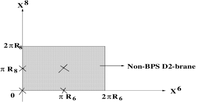
We shall consider type IIA theory on this particular Calabi-Yau orbifold $T^{6}/{\sf Z\!\!Z}^{(1)}_{2}\otimes{\sf Z\!\!Z}^{(2)}_{2}$. We take a non-BPS D1-brane of this theory and wrap it along $X^{9}$ such that it stretches over a fundamental interval $[0,2\pi R_{9}]$. The other eight spatial coordinates of this D-string are as given below :

$$(X^{1},X^{2},X^{3},X^{4},X^{5},X^{6},X^{7},X^{8})=(b_{1},b_{2},b_{3},a_{4},a_{5},0,0,0)\,,$$

where $a_{i}$ and $b_{k}$ are arbitrary numbers. Clearly the above configuration is invariant under ${\cal I}_{4}$ but not under ${\cal I}_{4}^{\;\prime}$. The image of the D-string under ${\cal I}_{4}^{\;\prime}$ is located at

$$(X^{1},X^{2},X^{3},X^{4},X^{5},X^{6},X^{7},X^{8})=(b_{1},b_{2},b_{3},-a_{4},-a_{5},\pi R_{6},0,\pi R_{8})\,.$$

Thus the original D-string together with its ${\cal I}_{4}^{\;\prime}$-image constitute an ${\cal I}_{4}\otimes{\cal I}_{4}^{\;\prime}$-invariant configuration (See Fig.1). Since the coordinates of the D-string and its ${\cal I}_{4}^{\;\prime}$ image in the non-compact directions $X^{1},X^{2},X^{3}$ must be identical, we see that this represents a single object in the orbifold theory. The physical interpretation of this object can be found by examining its charge quantum numbers. As is well known, a non-BPS D-string of type IIA string theory does not carry any bulk RR charge. However, if a D-string passes through an orbifold fixed point then it carries twisted sector RR charge associated with that fixed point[5, 20]. In the language of Calabi-Yau manifold, twisted sector RR charges are carried by BPS D2-branes wrapped on the (collapsed) 2-cycle associated with that given fixed point. Thus the D-string system, after orbifolding, carries charges corresponding to BPS 2-branes wrapped on various 2-cycles. Since it describes a single object, and is non-BPS, the natural interpretation of this object is that it describes a single BPS 2-brane, wrapped on a non-supersymmetric 2-cycle of the Calabi-Yau manifold. In the orbifold limit, this 2-cycle (of minimal area) collapses to a line.

Figure 1: Location of Non-BPS D-string and its ${\cal I}_{4}^{\;\prime}$-image in the $X^{6}$- $X^{8}$ and $X^{4}$-$X^{5}$ plane. D-strings are also present at the images of $O$ under translation by $2\pi R_{i}$ along $X^{i}$, e.g. at the point $Q$.

2.3 Region of Stability in Moduli Space

Next we are going to determine the region of stability in the moduli space for this particular system. Throughout our discussion we shall restrict ourselves to tree level of open string theory. Also, to simplify the discussion, in this subsection we shall work on the 4-fold cover of the orbifold, namely on the original torus $T^{6}$, although we shall ensure that we always work with configurations which are ${\cal I}_{4}$ and ${\cal I}_{4}^{\;\prime}$ invariant. Thus the various mass formulæ  we shall be writing down will refer to the masses of the corresponding systems on $T^{6}$ before orbifold projection.

Typically, the instability of the system arises due to open strings stretched between the D-string and one of its images developing a tachyonic mode. This involves images of the D-string under ${\cal I}_{4}^{\;\prime}$, as well as under translation by $2\pi R_{i}$ along $X^{i}$ for ($4\leq i\leq 8$). Since the physics of the instability arising due to open string stretched between the D-string and its image under translation is identical to that in the case of K3 orbifold, and can be analysed in a manner similar to that discussed in ref.[20], we shall concentrate on the instability arising due to the open string stretched between the D-string and its ${\cal I}_{4}^{\;\prime}$ image. In this case the relevant part of the moduli space is effectively two dimensional, spanned by $R_{6}$ and $R_{8}$, controlling the distance between the D-string and its ${\cal I}_{4}^{\;\prime}$-image. The open strings stretched between the D-string and its ${\cal I}_{4}^{\;\prime}$ image have been denoted as ${OP}$ and ${PQ}$ in Fig.1.

The general strategy for this kind of analysis has been stated in [51]. As a first step, let us determine the effective $(mass)^{2}$ of the winding mode tachyon coming from the open string ${OP}$ and ${PQ}$. From Fig. 1 we see that it is given by :

$$m_{T(1)}^{2}=\Big{(}\frac{a_{4}}{\pi}\Big{)}^{2}+\Big{(}\frac{a_{5}}{\pi}\Big{)}^{2}+\Big{(}\frac{1}{2}R_{6}\Big{)}^{2}+\Big{(}\frac{1}{2}R_{8}\Big{)}^{2}-\frac{1}{2}$$ (2.2)

in $\alpha^{\prime}=1$ unit which we shall be using throughout this paper. Since $a_{4}$ and $a_{5}$ are degress of freedom of the D-strings one requires that there should be no tachyons for any values of $a_{4}$ and $a_{5}$. The most stringent condition comes from

$$a_{4}=\;a_{5}=\;0\,.$$ (2.3)

Then the condition for the absence of tachyon from the winding modes ($m_{T(1)}^{2}\geq 0$) is given by :

$$R_{6}^{2}+R_{8}^{2}\geq 2\,.$$ (2.4)

The critical curve in the $R_{6}$-$R_{8}$ plane, where the tachyon is massless, is given by

$$R_{6}^{2}+R_{8}^{2}\;=\;2\,.$$ (2.5)

In the next section (section 3) we shall find the possible decay products of these ${\cal I}_{4}^{\;\prime}$-invariant pair of non-BPS D-strings by applying the conservation of energy and bulk and twisted RR charges. Anticipating the results of the section 3, $-$ that the instability of pair of non-BPS D-strings for $R_{6}^{2}+R_{8}^{2}<2$ represents the possibility of decay into a pair of ${\cal I}_{4}^{\;\prime}$-invariant non-BPS D3-branes extended in $X^{6},X^{8}$ and $X^{9}$ directions, $-$ we shall now determine the phase diagram of this system on $R_{6}$-$R_{8}$ plane. As we shall see in section 3, conservation of twisted sector RR charge (after orbifolding) requires that on one of the non-BPS D3-branes there are ${\sf Z\!\!Z}_{2}$ Wilson lines along $X^{6}$ and $X^{8}$ directions. The zero momentum mode of the open string with both ends on the same D3-brane is projected out by requiring invariance under ${\cal I}_{4}$, and the potentially tachyonic mode on this system comes from open strings stretched between the pair of D3-branes carrying half unit of momenta along $X^{6}$ and $X^{8}$ directions. The mass of this mode when the two D3-branes coincide in the $X^{1},\ldots X^{5},X^{7}$ directions, is given by:

$$m_{T(3)}^{2}=\Big{(}\frac{1}{2R_{6}}\Big{)}^{2}+\Big{(}\frac{1}{2R_{8}}\Big{)}^{2}-\frac{1}{2}$$ (2.6)

Thus the condition for absence of tachyonic modes on the D3-brane system is:

$$\frac{1}{R_{6}^{2}}+\frac{1}{R_{8}^{2}}\;\geq\;\;2$$ (2.7)

Figure 2: Phase diagram on $R^{6}$-$R^{8}$ plane. $A$ denotes the curve $R_{6}^{-2}+R_{8}^{-2}=2$; $B$ denotes the curve $R_{6}R_{8}=1$ and $C$ represents the curve $R^{2}_{6}+R^{2}_{8}=2$. In region I the D3-brane pair is stable and the D1-brane pair is unstable whereas in region II D1-brane pair is stable and the D3-brane pair is unstable. In region III the D1-brane pair is stable and the D3-brane pair is metastable, whereas in region IV the D3-brane pair is stable and the D1-brane pair is metastable.

Let us further write down the mass formula for the pair of D1-branes as well as for the pair of D3-branes. The mass of a pair of non-BPS D-strings wrapped along $X^{9}$ is given by:

$$M_{D1}=2\cdot\frac{1}{2\pi g}\sqrt{2}\cdot 2\pi R_{9}=\frac{2\sqrt{2}}{g}R_{9}$$ (2.8)

where $g$ is the closed string coupling constant and the factor of $\sqrt{2}$ is due to the non-BPS nature of the D-string. Similarly the mass of the non-BPS D3-brane pair is given by:

$$M_{D3}=2\cdot\frac{1}{(2\pi)^{3}g}\cdot\sqrt{2}\cdot(2\pi)^{3}R_{6}R_{8}R_{9}=\frac{2\sqrt{2}R_{6}R_{8}R_{9}}{g}$$ (2.9)

Comparing eqs.(2.8) and (2.9) we see that

$$M_{D1}\leq M_{D3}\qquad\hbox{for}\qquad R_{6}R_{8}\geq 1\,.$$ (2.10)

Note that for $R_{6}R_{8}=1$, these two masses become degenerate.

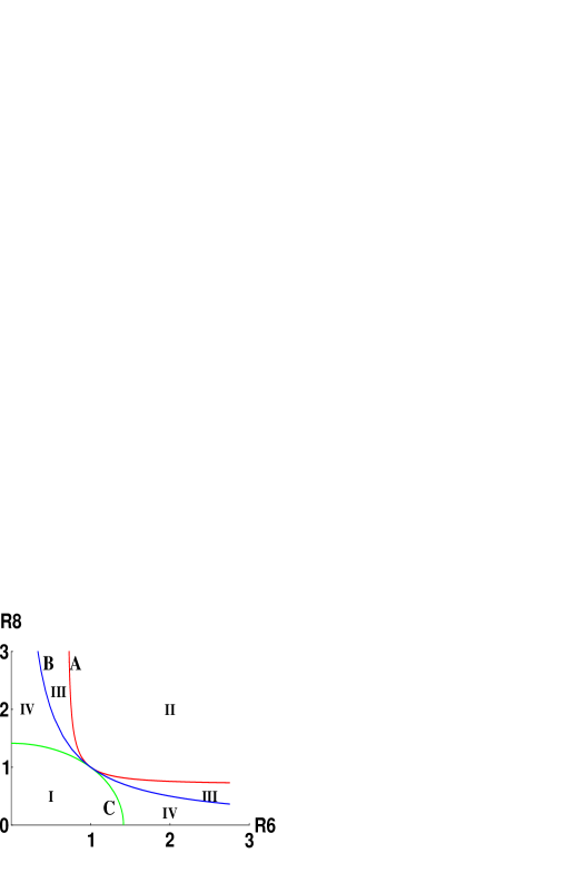
The various curves found during the analysis have been plotted in the phase diagram of Fig. 2. The curve $R_{6}R_{8}=1$ is the curve $B$ in Fig. 2. The equality in (2.7) has been represented as the curve $A$, and the curve $C$ denotes the circle given by eq.(2.5). There are four regions of interest altogether in this phase diagram:

1. $R_{6}^{2}+R_{8}^{2}<2$ (Region I)

   Here

   $$R_{6}^{-2}+R_{8}^{-2}={4(R_{6}^{2}+R_{8}^{2})\over(R_{6}^{2}+R_{8}^{2})^{2}-(R_{6}^{2}-R_{8}^{2})^{2}}>2\,.$$

   Thus the D3-brane pair does not have tachyon. Furthermore

   $$R_{6}R_{8}=\displaystyle{{R^{2}_{6}+R^{2}_{8}-(R_{6}-R_{8})^{2}\over 2}<1}\;,$$

   and hence the D3-brane pair is lighter than the D1-brane pair. Thus the D3-brane pair is stable. On the other hand in this region the D-string pair has tachyon and hence is unstable.

2. $R_{6}^{-2}+R_{8}^{-2}<2$ (Region II)

   Here

   $$R_{6}^{2}+R_{8}^{2}={4(R_{6}^{-2}+R_{8}^{-2})\over(R_{6}^{-2}+R_{8}^{-2})^{2}-(R_{6}^{-2}-R_{8}^{-2})^{2}}>2\,.$$

   Thus the D-string pair does not have tachyon. Furthermore

   $$R_{6}R_{8}=\displaystyle{{2\over R^{-2}_{6}+R^{-2}_{8}-(R_{6}^{-1}-R_{8}^{-1})^{2}}>1}\;,$$

   and hence the D-string pair is lighter than the D3-brane pair. Thus the D-string pair is stable. But in this region the D3-brane pair has a tachyonic mode and hence is unstable.

3. $R_{6}R_{8}>1$ and $R_{6}^{-2}+R_{8}^{-2}>2$ (Region III)

   Here $R_{6}^{2}+R_{8}^{2}=(R_{6}^{-2}+R_{8}^{-2})R_{6}^{2}R_{8}^{2}>2$. Thus both D1 and D3-brane pairs are free from tachyonic mode. But $M_{D3}>M_{D1}$. Thus the D-string pair is stable, whereas the D3-brane pair is in a metastable state.

4. $R_{6}R_{8}<1$ and $R_{6}^{2}+R_{8}^{2}>2$ (Region IV)

   Here $R_{6}^{-2}+R_{8}^{-2}=(R_{6}^{2}+R_{8}^{2})/(R_{6}^{2}R_{8}^{2})>2$. Thus in this region also both systems are free of tachyon. But now $M_{D1}>M_{D3}$. Therefore the D3-brane pair is stable and the D-string pair is in a metastable state.

Interestingly all three curves $A$, $B$, $C$ meet at one point viz.  at the critical radii $(R_{6},R_{8})=(1,1)$. As we shall see in section 4, at this point the D-string pair can be deformed to the D3-brane pair via a marginal deformation. Across any other point along the curve $B$, the transition from one to the other is first order (metastable $\to$ stable). As neither system contains a relevant perturbation, it is not clear if the arguments based on renormalization group flow[53, 54] can be used to describe this transition.

Before we end this section, we should remind the reader that in our analysis we have ignored the possibility of tachyons appearing in various other ways. Thus for example, requiring that there is no tachyonic mode on the D1-brane system from open strings stretched between a D1-brane and its image under translation along $X^{i}$ ($6\leq i\leq 8$) gives the constraints[20]:

$$R_{i}\geq{1\over\sqrt{2}}\,,\qquad 6\leq i\leq 8\,.$$ (2.11)

On the other hand, requiring that open string states with both ends on the same D-string, but carrying momentum along $X^{9}$ does not give rise to a tachyonic mode gives

$$R_{9}\leq\sqrt{2}\,.$$ (2.12)

As shown in ref.[20], beyond these ranges of $R_{i}$ the system becomes unstable against decay into a pair of BPS states. Throughout our analysis we shall work in regions of the moduli space where eqs.(2.11) and (2.12) are satisfied.

Now we turn our attention to various conservation laws to verify that the decay modes described above are indeed possible.

3 Determination of Decay Products of Non-BPS D-string Pair

In this section we shall show that a pair of non-BPS D-strings as shown in Fig. 1 (with $a_{4}=a_{5}=0$) can decay into a pair of non-BPS D3-branes for $R_{6}R_{8}<1$, satisfying the conservation of energy, bulk RR-charge and twisted RR-charge. Then we shall find a physical interpretation of the final state D3-branes as wrapped D-branes on the Calabi-Yau 3-fold.

3.1 Verification of the Conservation Laws

In this section we shall map our problem to an equivalent type IIB description to make calculations simpler. For this we shall perform a T-duality transformation ${{\cal T}}_{9}$ along the coordinate $X^{9}$ to get type IIB string theory on a dual torus labelled by $X^{4},\ldots X^{8},\widetilde{X}^{9}$. In that case,

$$\mbox{IIA on $T^{6}/{\cal I}_{4}\otimes{\cal I}_{4}^{\;\prime}$}\;\;\stackrel{{\scriptstyle{\cal T}_{9}}}{{\longrightarrow}}\;\;\mbox{IIB on $T^{6}/(\widetilde{\cal I}_{4}\cdot(-1)^{F_{L}}\otimes{\cal I}_{4}^{\;\prime})$}$$

where $\widetilde{\cal I}_{4}$ denotes the transformation:

$$\widetilde{\cal I}_{4}:\qquad(X^{4},\ldots X^{8},\widetilde{X}^{9})\to(X^{4},X^{5},-X^{6},-X^{7},-X^{8},-\widetilde{X}^{9})\,,$$

and $(-1)^{F_{L}}$ changes the sign of all the (R,NS) and (R,R) sector states. We shall continue to denote by ${\cal I}_{4}$ the transformation $\widetilde{\cal I}_{4}\cdot(-1)^{F_{L}}$ in the type IIB string theory, as this is just the image of the transformation ${\cal I}_{4}$ in the type IIA theory. Also under the duality ${{\cal T}}_{9}$,

$$\mbox{Non-BPS D1-brane (along $X^{9}$) of IIA}\;\;\stackrel{{\scriptstyle{\cal T}_{9}}}{{\longrightarrow}}\;\;\mbox{Non-BPS D0-brane of IIB}$$

$$\mbox{Non-BPS D3-brane (along $X^{6}$-$X^{8}$-$X^{9}$) of IIA}\;\;\stackrel{{\scriptstyle{\cal T}_{9}}}{{\longrightarrow}}\;\;\mbox{Non-BPS D2-brane (along $X^{6}$-$X^{8}$) of IIB}$$

Figure 3: Non-BPS D0-brane of type IIB and its ${\cal I}_{4}^{\;\prime}$-image in the interval $0\leq x^{6}<2\pi R_{6}$, $0\leq x^{8}<2\pi R_{8}$. $`\times$’ denotes the fixed points of ${\cal I}_{4}$ on $X^{6}$-$X^{8}$ plane.

Thus, in IIB description, the initial system consists of non-BPS D0-branes at $(X^{6},X^{8})=(0,0)$ and $(\pi R_{6},\pi R_{8})$ (see Fig.3). From now on, unless otherwise stated, we shall use the IIB description throughout this section 3.1. In applying conservation laws of RR charges, we shall find it convenient to work with a double cover of the system, where we have modded out type IIB string theory on $T^{6}$ by ${\cal I}_{4}$ but not by ${\cal I}_{4}^{\;\prime}$. Since ${\cal I}_{4}^{\;\prime}$ does not have any fixed point, and hence does not introduce any new massless state and twisted sector RR charge, ensuring conservation of RR charge before ${\cal I}_{4}^{\;\prime}$ modding is sufficient to guarantee its conservation after ${\cal I}_{4}^{\;\prime}$ modding. On the other hand for applying conservation of energy, we shall work with the four fold cover of the system, $-$ on the original torus $T^{6}$. Of course, at every stage of the analysis we shall ensure that we have a system that is invariant under both ${\cal I}_{4}$ and ${\cal I}_{4}^{\;\prime}$, so that we can mod out the configuration by these transformations at the end.

Figure 4: Non-BPS D2-brane of type IIB in the interval $0\leq x^{6}<2\pi R_{6}$, $0\leq x^{8}<2\pi R_{8}$. ‘$\times$’ denotes the fixed points of ${\cal I}_{4}$.

The non-BPS D0-branes, situated at (0,0) and $(\pi R_{6},\pi R_{8})$, do not carry any bulk RR charge, but carry twisted sector RR charge[5]. We shall denote by $q_{(a_{6},a_{8})}$ the twisted sector charge at the fixed point $(a_{6},a_{8})$ in the $(X^{6},X^{8})$ plane. The charge will be normalized such that a non-BPS D0-brane of IIB, placed at any of the fixed points of ${\cal I}_{4}$, carries unit twisted sector RR charge associated with that fixed point. Thus our initial state has charges:

$$q_{(0,0)}^{(in)}=q_{(\pi R_{6},\pi R_{8})}^{(in)}=1,\qquad q_{(0,\pi R_{8})}^{(in)}=q_{(\pi R_{6},0)}^{(in)}=0\,.$$ (3.1)

The final decay product must also carry this charge. We shall consider non-BPS D2-branes of type IIB theory in the $X^{6}-X^{8}$ plane as our candidate for decay product. Fig.4 shows the configuration of a single non-BPS D2-brane in the range $0\leq x^{6}<2\pi R_{6}$, $0\leq x^{8}<2\pi R_{8}$. This is by itself an ${\cal I}_{4}^{\;\prime}$-invariant configuration. Although this does not carry any bulk RR charge, it carries twisted sector RR charges associated with every fixed point that it passes through. These charges can be computed using the boundary state formalism of ref.[28]. If $\theta_{6}$ and $\theta_{8}$ denote the Wilson lines on the 2-brane along $X^{6}$ and $X^{8}$ respectively, taking values 0 or $\pi$ due to the requirement of ${\cal I}_{4}$ invariance, then the twisted sector charges carried by the brane is given by:

$$q_{(0,0)}={1\over 2}\epsilon,\qquad q_{(0,\pi R_{8})}={1\over 2}\epsilon e^{i\theta_{8}},\qquad q_{(\pi R_{6},0)}={1\over 2}\epsilon e^{i\theta_{6}},\qquad q_{(\pi R_{6},\pi R_{8})}={1\over 2}\epsilon e^{i(\theta_{6}+\theta_{8})}\,,$$ (3.2)

where $\epsilon$ can take values $\pm 1$. This result, including the overall normalization factor of $(1/2)$ appearing in the expression for the charges, can be read out from the expression for the boundary state of the 2-brane as given in ref.[28]. This normalization factor of (1/2) can also be derived from the fact that in type IIB string theory on $T^{6}/{\cal I}_{4}$, the D2-brane can be continuously deformed, via tachyon condensation, to a D-string at $X^{6}=0$, and a $\bar{\rm D}$-string at $X^{6}=\pi R_{6}$, both stretched along $x^{8}$[20]. Each of these D-strings carry half unit of twisted sector charge at the fixed points through which they pass[3, 55]. Since a continuous deformation cannot change the value of RR charge quantum numbers, the D2-brane before tachyon condensation must also carry half unit of twisted sector charge at each of the four fixed points (0,0), $(0,\pi R_{8})$, $(\pi R_{6},0)$ and $(\pi R_{6},\pi R_{8})$.

Since ${\cal I}_{4}^{\;\prime}$ exchanges the points (0,0) with $(\pi R_{6},\pi R_{8})$ and $(0,\pi R_{8})$ with $(\pi R_{6},0)$, we see from (3.2) that in order to get an ${\cal I}_{4}^{\;\prime}$ invariant configuration, we must have $\theta_{6}=\theta_{8}=0$ or $\theta_{6}=\theta_{8}=\pi$.

Now let us take $N$ such coincident D2-branes. We shall slightly generalise our notation by replacing $(\epsilon,\;{\theta}_{6},\;{\theta}_{8})$ in the above expressions by $(\epsilon^{(k)},\;{\theta}_{6}^{(k)},\;{\theta}_{8}^{(k)})$ respectively ($k=1,\cdots,N$). Thus for $N$ such coincident branes we have:

$$\displaystyle q^{(tot)}_{(0,0)} = {1\over 2}\sum_{k=1}^{N}\epsilon^{(k)}$$

$$q^{(tot)}_{(0,\pi R_{8})} = {1\over 2}\sum_{k=1}^{N}\epsilon^{(k)}e^{i\,{\theta}_{8}^{(k)}}$$

$$q^{(tot)}_{(\pi R_{6},\pi R_{8})} = {1\over 2}\sum_{k=1}^{N}\epsilon^{(k)}e^{i\,({\theta}_{6}^{(k)}\;+\;{\theta}_{8}^{(k)})}$$

$$q^{(tot)}_{(\pi R_{6},0)} = {1\over 2}\sum_{k=1}^{N}\epsilon^{(k)}e^{i\,{\theta}_{6}^{(k)}}$$ (3.3)

Again, ${\cal I}_{4}^{\;\prime}$ invariance of individual branes requires $\theta_{6}^{(k)}=\theta^{(k)}_{8}=0$ or $\pi$ for each $k$. Hence applying charge conservation, and using eqs.(3.1) and (3.1), we get:

$$\displaystyle\sum_{k=1}^{N}\epsilon^{(k)}\,e^{i\,{\theta}_{8}^{(k)}} = 0$$ (3.4)

$$\sum_{k=1}^{N}\epsilon^{(k)}\,e^{i\,{\theta}_{6}^{(k)}} = 0$$ (3.5)

$$\sum_{k=1}^{N}\epsilon^{(k)} = 2$$ (3.6)

$$\sum_{k=1}^{N}\epsilon^{(k)}\,e^{i\,({\theta}_{6}^{(k)}\;+\;{\theta}_{8}^{(k)})} = 2$$ (3.7)

Since $\epsilon^{(k)}=\pm 1$, from (3.6) we can easily see that $N$ must be an even integer. It is also easy to demonstrate that eqs.(3.4)-(3.7) admit solutions for any even integer $N$. For example, for $N=2$ we get the following consistent set of solutions:

$$\epsilon^{(1)}=\epsilon^{(2)}=+\,1\,,$$ (3.8)

$$\mbox{Either}\qquad{\theta}_{6}^{(1)}=0,\;\;{\theta}_{8}^{(1)}=0;\qquad{\theta}_{6}^{(2)}=\pi,\;\;{\theta}_{8}^{(2)}=\pi$$ (3.9)

$$\mbox{or}\qquad{\theta}_{6}^{(1)}=\pi,\;\;{\theta}_{8}^{(1)}=\pi;\qquad{\theta}_{6}^{(2)}=0,\;\;{\theta}_{8}^{(2)}=0$$ (3.10)

As is evident from (3.9) and (3.10), one of the 2-branes carries ${\sf Z\!\!Z}_{2}$ Wilson lines along $X^{6}$ and $X^{8}$. From this solution, we can construct solutions for any even $N$ by adding pairs of branes with same $\theta_{6}$ and $\theta_{8}$ and opposite values of $\epsilon$. Other solutions are also possible.

Now we want to compare the masses of the initial and the final system of D-branes. Before any orbifold projection, the mass of $N=2\,m\,(m\in{\sf Z\!\!Z}_{+})$ non-BPS D2-branes in a fundamental cell $X^{6}\in[0,2\pi\,R_{6}]$, $X^{8}\in[0,2\pi\,R_{8}]$ (see fig. 4) is equal to $\displaystyle\frac{N\,\sqrt{2}\,R_{6}\,R_{8}}{g}$, whereas the mass of the initial configuration of a pair of non-BPS D0-branes is $\displaystyle\frac{2\,\sqrt{2}}{g}$. Demanding that the initial system has higher mass than the final state, we obtain

$$R_{6}\,R_{8}\leq\frac{2}{N},$$ (3.11)

This condition is least stringent for $N=2$, and hence this is the generic decay channel of the original system in its region of instability. Indeed, for $N=2$, eq.(3.11) is automatically satisfied whenever $R_{6}^{2}+R_{8}^{2}\leq 2$, $-$ the region where the original D0-brane pair develops a tachyonic mode. In addition, in more restricted regions of the moduli space, given by eq.(3.11) for $N\geq 4$, additional decay channels open up in which the original system decays to four or more non-BPS D-branes. We should of course keep in mind that once one of the radii is sufficiently small, we violate (2.11), and decay channels into BPS branes also open up.

For $N=2$, the equality in (3.11) and eq.(2.5) are satisfied simultaneously for $(R_{6},R_{8})=(1,1)$. As we shall see in the next section, there is an exactly marginal deformation which interpolates between the initial and the final system at this critical radii for $N=2$.

3.2 Interpretation of the Final State

So far we have analysed the system before modding it out by ${\cal I}_{4}^{\;\prime}$. As has already been noted, after modding out by ${\cal I}_{4}^{\;\prime}$, the initial system describes a single brane configuration as it has only one set of degrees of freedom describing its movement in the non-compact directions. In contrast, each of the type IIB D2-brane configurations in the final state is ${\cal I}_{4}$ and ${\cal I}_{4}^{\;\prime}$ invariant by itself, and hence can move in the non-compact directions independently of the other D-branes. Thus the final state describes a set of $N$ independent objects.

In order to find the physical interpretation of these objects, we examine the RR charges carried by each of these objects. For this we go back to the type IIA description by performing T-duality along $X^{9}$. Under this duality, a non-BPS D2-brane of IIB gets mapped to a non-BPS D3-brane of IIA spanning the $X^{6}-X^{8}-X^{9}$ directions. The brane does not carry any bulk RR charge, but it carries twisted sector RR charges associated with each fixed point through which it passes. Since these RR charges are carried by BPS 2-branes wrapped on homologically non-trivial 2-cycles, it will be natural to interprete the non-BPS 3-brane as a 2-brane wrapped on some complicated 2-cycle of the Calabi-Yau manifold. However this interpretation cannot be correct. To see this, let us deform all the radii $R_{4},\ldots R_{9}$ to very large values. This makes the non-BPS 3-brane unstable, but it continues to exist as a classical solution of the equations of motion. Clearly in this region this cannot be interpreted as a BPS 2-brane wrapped on a 2-cycle, since it occupies a 3-dimensional subspace. Instead it can be interpreted as a bound state of a D4-brane $\bar{\rm D}$4-brane pair[3, 6], each wrapped on a K3 subspace of the Calabi-Yau orbifold spanned by $X^{6},\ldots X^{9}$. The two D4-branes must carrying different amounts of magnetic flux through the homology two cycles, so that after combining the effect of the magnetic flux with the effect of the non-trivial anti-symmetric tensor field flux through the 2-cycles[56], we recover the correct RR charges of the brane. Equivalently, we can think of each non-BPS 3-brane as a single D4-brane wrapped on a trivial 4-cycle, but carrying nontrivial magnetic flux through various homology 2-cycles.

4 Conformal Field Theory at the Critical Radii

In this section we shall show that at the critical radii $R_{6}=R_{8}=1$, there is an exactly marginal deformation which interpolates between the D3-brane pair and the D1-brane pair. We shall carry out this analysis before either ${\cal I}_{4}$ or ${\cal I}_{4}^{\;\prime}$ projection, but making sure that at every stage of the analysis the configuration under study is invariant under ${\cal I}_{4}$ and ${\cal I}_{4}^{\;\prime}$.

We shall find it more convenient to start with the BCFT describing the D3-brane pair spanning $X^{6}$-$X^{8}$-$X^{9}$ directions, and identify an ${\cal I}_{4}$ and ${\cal I}_{4}^{\;\prime}$ invariant marginal perturbation which takes this BCFT to the BCFT describing the D1-brane pair along $X^{9}$ direction. The relevant part of the BCFT at the critical radii before we switch on the perturbation is described by a pair of scalar fields $X^{i}\equiv X^{i}_{L}+X^{i}_{R}$ for $i=6,8$ and their left- and right-moving superpartners $\psi^{i}_{L},\psi^{i}_{R}$. These fields satisfy Neumann boundary conditions on the real line, given by:

$$(X^{i}_{L})_{B}=\>(X^{i}_{R})_{B}\equiv\frac{1}{2}\>X^{i}_{B};\qquad(\psi^{i}_{L})_{B}=\>(\psi^{i}_{R})_{B}\equiv\>\psi^{i}_{B}.$$ (4.1)

Besides these there are other scalar fields and their fermionic superpartners corresponding to the other coordinates, and also bosonic and fermionic ghost fields. But they will play no role in our analysis.

The other part of the BCFT which will be important for our analysis is the Chan Paton (CP) factor. Open string spectrum on each non-BPS D3-brane comes from two CP sectors[7]: ${\rm I\!I}_{2}$ and $\sigma_{1}$ ($2\times 2$ Pauli matrix) — these will be called internal CP factors. For a pair of non-BPS D3-branes, there also exists a set of external CP factors : ${\rm I\!I}_{2}$, $\Sigma_{1}$, $\Sigma_{2}$, and $\Sigma_{3}$ ($2\times 2$ Pauli matrices). ($\Sigma_{1}$, $\Sigma_{2}$) CP sectors correspond to open strings stretched between different non-BPS D3-branes, and (${\rm I\!I}_{2}$, $\Sigma_{3}$) correspond to open strings with both ends on the same D3-brane. The internal and external CP factors commute with each other.

Due to the presence of ${\sf Z\!\!Z}_{2}$ Wilson lines along $X^{6}$ and $X^{8}$ on one of the D3-branes, the open string states with two ends on two different D3-branes are anti-periodic under $X^{6}\to X^{6}+2\pi R_{6}$ and under $X^{8}\to X^{8}+2\pi R_{8}$, and hence carry half integer units of momentum along $X^{6}$ and $X^{8}$. This can be restated as follows: the translation symmetry $X^{8}\to X^{8}+2\pi R_{8}$ ($X^{6}\to X^{6}+2\pi R_{6}$) under which we normally identify space to make $X^{8}$ ($X^{6}$) compact, acts on the open string states via conjugation by $\Sigma_{3}$. Under this conjugation, CP sectors ${\rm I\!I}_{2}$ and $\Sigma_{3}$, representing open strings with both ends on the same D3-brane, remain invariant, but CP sectors $\Sigma_{1}$ and $\Sigma_{2}$, representing open strings with two ends on two different branes, change sign. This is exactly what we require.

Our next task is to determine the action of ${\cal I}_{4}$ and ${\cal I}_{4}^{\;\prime}$ on various operators of the BCFT, so that we can identify ${\cal I}_{4}$ and ${\cal I}_{4}^{\;\prime}$ invariant vertex operators. On the coordinates $X^{6}$ and $X^{8}$ and their fermionic partners, the action of ${\cal I}_{4}$ and ${\cal I}_{4}^{\;\prime}$ has been specified in eqs.(2.1) and (2.1); thus we only need to determine their action on the CP factors. We can divide this into two parts: the action on the internal CP factor, and that on the external CP factor. The action on the internal CP factor can be determined by taking a single D3 brane, and identifying an appropriate 2-point coupling between a closed string state and an open string state[20]. Since we know the transformation properties of the closed string states under ${\cal I}_{4}$ and ${\cal I}_{4}^{\;\prime}$, this determines the transformation properties of open string states under ${\cal I}_{4}$ and ${\cal I}_{4}^{\;\prime}$, and hence their action on the internal CP factor. This procedure has been illustrated in ref.[20]; hence here we shall quote the final result. Both ${\cal I}_{4}$ and ${\cal I}_{4}^{\;\prime}$ conjugates internal CP factor by $\sigma_{3}$. Thus they leave states with internal CP factor ${\rm I\!I}_{2}$ unchanged, and change the sign of the states with internal CP factor $\sigma_{1}$.

Let us now turn to the action of ${\cal I}_{4}$ and ${\cal I}_{4}^{\;\prime}$ on the external CP factors. Since both ${\cal I}_{4}$ and ${\cal I}_{4}^{\;\prime}$ leave individual D3-branes unchanged, they must leave unchanged CP factors ${\rm I\!I}_{2}$ and $\Sigma_{3}$, and hence can at most induce a rotation about the 3-axis on the external CP factors. Since $({\cal I}_{4})^{2}$ acts as identity on the fields, it must also act as identity on the CP factor in order that it is an order two transformation. This leaves us with two choices: either it acts as conjugation by $\Sigma_{3}$, and changes the sign of $\Sigma_{1}$ and $\Sigma_{2}$, or it leaves all external CP factors invariant. Both choices are allowed. After modding out the theory by ${\cal I}_{4}$, these two choices can be shown to be related to the choice of relative sign of $\epsilon^{(1)}$ and $\epsilon^{(2)}$ in eqs.(3.1). From eq.(3.8) we see that we need $\epsilon^{(1)}=\epsilon^{(2)}$; this can be shown to correspond to choosing the action of ${\cal I}_{4}$ to be trivial on all the external CP factors. For the time being we shall proceed with this assumption, but later we shall consider the other choice, and show how this corresponds to choosing $\epsilon^{(1)}=-\epsilon^{(2)}$. (The most straightforward way of seeing this is to construct the boundary state of the D3-branes characterized by $\epsilon$, $\theta_{6}$ and $\theta_{8}$, and then compute the open string partition function by taking the inner product between two such boundary states. But we shall follow a shorter, more intuitive path.)

Next we turn to the action of ${\cal I}_{4}^{\;\prime}$ on the external CP factors. For this note that the action of $({\cal I}_{4}^{\;\prime})^{2}$ on various fields is given as follows:

$$({\cal I}_{4}^{\;\prime})^{2}:\qquad X^{6}\to X^{6},\quad X^{8}\to X^{8}+2\pi R_{8},\quad\psi^{6}\to\psi^{6},\quad\psi^{8}\to\psi^{8}\,.$$ (4.2)

Recall now that $X^{8}\to X^{8}+2\pi R_{8}$ acts as identity on all the open string states only if it is accompanied by the conjugation of external CP factors by $\Sigma_{3}$. Thus in order that ${\cal I}_{4}^{\;\prime}$ is an order two transformation, $({\cal I}_{4}^{\;\prime})^{2}$ must conjugate external CP factors by $\Sigma_{3}$. Hence ${\cal I}_{4}^{\;\prime}$ itself must conjugate the external CP factors by a square root of $\Sigma_{3}$. Furthermore, we have already seen that it should leave the external CP factors ${\rm I\!I}_{2}$ and $\Sigma_{3}$ unchanged. This leaves us with two possible choices: conjugation by $\exp(\pm i\pi\Sigma_{3}/4)$. They give equivalent results. For definiteness, we shall take this to be $\exp(i\pi\Sigma_{3}/4)$.

With these rules we are now in a position to construct the ${\cal I}_{4}$ and ${\cal I}_{4}^{\;\prime}$ invariant vertex operators. At $R_{6}=R_{8}=1$, the lowest energy states of the open strings, carrying internal CP factor $\sigma_{1}$, external CP factors $\Sigma_{1}$ or $\Sigma_{2}$, and momenta $\pm{1\over 2}$ along $X^{6}$ and $X^{8}$, become massless. Before requiring ${\cal I}_{4}$ and ${\cal I}_{4}^{\;\prime}$ invariance, the vertex operator of one such open string state in the (0,0) picture[57] is given by:

$$(\psi^{6}_{B}+\psi^{8}_{B})\exp({i\over 2}(X^{6}_{B}+X^{8}_{B}))\otimes\sigma_{1}\otimes\Sigma_{1}\,.$$ (4.3)

The complete ${\cal I}_{4}$ and ${\cal I}_{4}^{\;\prime}$ invariant vertex operator can be constructed by adding to it its transforms under ${\cal I}_{4}$, ${\cal I}_{4}^{\;\prime}$ and ${\cal I}_{4}\cdot{\cal I}_{4}^{\;\prime}$. This is given by

$$\displaystyle V^{(0)}_{T} \propto \frac{1}{2}\,({\psi}^{6}_{B}\>+\>{\psi}^{8}_{B})\,\Big{[}\,e^{i({X}^{6}_{B}\>+\>{X}^{8}_{B})/2}\;+\;e^{-\,i({X}^{6}_{B}\>+\>{X}^{8}_{B})/2}\,\Big{]}\otimes\sigma_{1}\otimes\Sigma_{1}$$ (4.4)

$$+ \>\frac{1}{2}\,({\psi}^{6}_{B}\>-\>{\psi}^{8}_{B})\,\Big{[}\,e^{i({X}^{6}_{B}\>-\>{X}^{8}_{B})/2}\;+\;e^{-\,i({X}^{6}_{B}\>-\>{X}^{8}_{B})/2}\,\Big{]}\otimes\sigma_{1}\otimes\Sigma_{2}$$

We now note that this perturbation is identical to the one described in ref.[51] in the context of marginal deformation of a BPS D-brane - $\bar{\rm D}$-brane system, with the only difference that there is an additional internal CP factor $\sigma_{1}$ attatched to each vertex operator. Since $\sigma_{1}$ commutes with all other operators, the presence of this operator does not affect the analysis, and one can show following ref.[51] that (4.4) corresponds to an exactly marginal operator. One can also follow the procedure of [51] to study how the spectrum of open strings changes under this deformation, and show that for a specific value of the deformation parameter the spectrum becomes identical to that of open strings living on a pair of D1-branes (along $X^{9}$) situated at diametrically opposite points of the torus spanned by $(X^{6},X^{8})$. Indeed, part of the spectrum of open strings living on the original non-BPS D3-brane pair, corresponding to CP factors ${\rm I\!I}_{2}\otimes{\rm I\!I}_{2}$, ${\rm I\!I}_{2}\otimes\Sigma_{3}$, $\sigma_{1}\otimes\Sigma_{1}$ and $\sigma_{1}\otimes\Sigma_{2}$, is identical to that living on a D3-$\bar{\rm D}$3 brane pair of IIB, and these states evolve under the marginal deformation in a manner identical to that described in [51]. These correspond to states living on a D1-$\bar{\rm D}$1 brane pair of IIB in the deformed theory, forming part of the expected spectrum of open strings on a D1-brane pair of IIA. The rest of the states on the D3-brane pair of IIA can be shown to evolve into the rest of the states on the D1-brane pair of IIA under this deformation. As the analysis is a straightforward generalization of the one carried out in [51], we shall not repeat it here.

Thus we conclude that the marginal deformation takes the original D3-brane pair to a D1-brane pair. The locations of the D1-branes can be determined as follows. The tachyon vertex operator in the zero picture is given in (4.4). Examining the $-1$ picture version of this vertex operator, and defining a complex tachyon field whose real and imaginary parts are proportional to the coefficients of $\Sigma_{1}$ and $\Sigma_{2}$ respectively in the $-1$ picture, as in [51], we get

$$T(X^{6},X^{8})\propto\sin({1\over 2}(X^{6}+X^{8}))+i\sin({1\over 2}(X^{6}-X^{8}))\,.$$ (4.5)

This has zeroes at $X^{6}=X^{8}=0$ and at $X^{6}=X^{8}=\pi$, showing that these are the locations of the D1-branes. This is consistent with the choice (3.8)-(3.10), since with this choice the net twisted sector charges are concentrated at $X^{6}=X^{8}=0$ and at $X^{6}=X^{8}=\pi$.

Now suppose we had made a different choice for the action of ${\cal I}_{4}$ on the external CP factors, namely that it changes the sign of the external CP factors $\Sigma_{1}$ and $\Sigma_{2}$. In that case, (4.4) would be replaced by

$$\displaystyle V^{(0)}_{T} \propto \frac{1}{2}\,({\psi}^{6}_{B}\>+\>{\psi}^{8}_{B})\,\Big{[}\,e^{i({X}^{6}_{B}\>+\>{X}^{8}_{B})/2}\;-\;e^{-\,i({X}^{6}_{B}\>+\>{X}^{8}_{B})/2}\,\Big{]}\otimes\sigma_{1}\otimes\Sigma_{1}$$ (4.6)

$$- \>\frac{1}{2}\,({\psi}^{6}_{B}\>-\>{\psi}^{8}_{B})\,\Big{[}\,e^{i({X}^{6}_{B}\>-\>{X}^{8}_{B})/2}\;-\;e^{-\,i({X}^{6}_{B}\>-\>{X}^{8}_{B})/2}\,\Big{]}\otimes\sigma_{1}\otimes\Sigma_{2}$$

This is still a marginal deformation, but would correspond to a tachyon field configuration:

$$T(X^{6},X^{8})\propto\cos({1\over 2}(X^{6}+X^{8}))-i\cos({1\over 2}(X^{6}-X^{8}))\,.$$ (4.7)

Thus now it has zeroes at $(X^{6}=0,X^{8}=\pi)$ and at $(X^{6}=\pi,X^{8}=0)$. This is where the final state D1-branes will be, and hence this is where the twisted sector charges will be concentrated. By examining eq.(3.1) we see that this corresponds to the choice

$$\epsilon^{(1)}=-\epsilon^{(2)}\,,$$ (4.8)

together with eqs.(3.9) and (3.10). This shows that the choice of how ${\cal I}_{4}$ acts on external CP factors is correlated with the choice of relative signs of $\epsilon^{(1)}$ and $\epsilon^{(2)}$, and that for our system, ${\cal I}_{4}$ acts trivially on the external CP factors.

As in ref.[51] one can deform the system away from the critical radii, and show that the final system continues to describe a D1-brane pair. This establishes that the D1-brane pair indeed decays into a D3-brane pair (and vice versa) across the region of stability $R_{6}R_{8}=1$.

Acknowledgement: We would like to thank Debashis Ghoshal, Dileep Jatkar, Suresh Govindarajan, Sunil Mukhi and B. Stefansky for useful discussions. J.M. would also like to thank The Department of Theoretical Physics, TIFR, India, for their hospitality, where part of this work was done. A.S. would like to thank the New High Energy Theory Center at Rutgers University, Center for Theoretical Physics at MIT, and the Erwin Schroedinger Institute, Vienna for hospitality where part of this work was done.

References

- [1] J. Polchinski, Phys. Rev. Lett. 75 4724 (1995), hep-th/9510017.
- [2] A. Sen, “Stable Non-BPS States in String Theory”, JHEP 06 (1998) 007, hep-th/9803194.
- [3] A. Sen, “Stable non-BPS bound states of BPS D-branes,” JHEP 08, 010 (1998) hep-th/9805019.
- [4] A. Sen, “Tachyon condensation on the brane antibrane system,” JHEP 08, 012 (1998) hep-th/9805170.
- [5] O. Bergman and M.R. Gaberdiel, “Stable Non-BPS D particles,” Phys. Lett. B441, 133 (1998) hep-th/9806155.
- [6] A. Sen, “SO(32) Spinors of Type I and Other Solitons on Brane-Antibrane Pair,” JHEP 09 (1998) 023, hep-th/9808141.
- [7] A. Sen, “Type I D-particle and its Interactions”, JHEP 10 (1998) 021, hep-th/9809111.
- [8] M. Frau, L. Gallot, A. Lerda, P. Strigazzi, “Stable Non-BPS D-branes in Type I String Theory”, Nucl. Phys. B564, 60 (2000), hep-th/9903123.
- [9] E. Eyras and S. Panda, “The spacetime life of a non-BPS D-particle,” hep-th/0003033.
- [10] Y. Lozano, “Non-BPS D-brane solutions in six dimensional orbifolds,” hep-th/0003226.
- [11] P. Brax, G. Mandal and Y. Oz, “Supergravity description of non-BPS branes,” hep-th/0005242.
- [12] M. Bertolini, P. Di Vecchia, M. Frau, A. Lerda, R. Marotta and R. Russo, “Is a classical description of stable non-BPS D-branes possible?,” hep-th/0007097.
- [13] K. Becker, M. Becker, A. Strominger, “Fivebranes, Membranes and Non-perturabive String Theory”, Nucl. Phys. B456, 130 (1995) hep-th/9507158.
- [14] M. R. Douglas and G. Moore, “D-branes, Quivers, and ALE Instantons,” hep-th/9603167.
- [15] M. R. Douglas, B. R. Greene and D. R. Morrison, “Orbifold resolution by D-branes,” Nucl. Phys. B506, 84 (1997) [hep-th/9704151].
- [16] A. Recknagel and V. Schomerus, “D-branes in Gepner Models”, Nucl. Phys. B531, 185 (1998); [hep-th/9712186].
- [17] M. Gutperle and Y. Satoh, “D-branes in Gepner models and supersymmetry,” Nucl. Phys. B543, 73 (1999) [hep-th/9808080].
-
[18]
I. Brunner, M. R. Douglas, A. Lawrence and C. Romelsberger,
“D-branes on the Quintic”,
[hep-th/9906200];
M. R. Douglas, B. Fiol and C. Romelsberger, “Stability and BPS branes,” [hep-th/0002037];
M. R. Douglas, B. Fiol and C. Romelsberger, “The spectrum of BPS branes on a noncompact Calabi-Yau,” [hep-th/0003263]. -
[19]
S. Govindarajan, T. Jayaraman and T. Sarkar,
“Worldsheet approaches to D-branes on supersymmetric cycles”,
[hep-th/9907131];
S. Govindarajan and T. Jayaraman, “On the Landau-Ginzburg description of boundary CFTs and special Lagrangian submanifolds,” [hep-th/0003242]. - [20] A. Sen, “BPS Branes on Non-Supersymmetric Cycles,” JHEP 12 021 (1998), [hep-th/9812031].
- [21] O. Bergman and M. Gaberdiel, “Non-BPS States in Heterotic-Type IIA Duality”, JHEP 03 013 (1999), [hep-th/9901014].
- [22] M. Gutperle, “Non-BPS D-branes and enhanced symmetry in an asymmetric orbifold,” hep-th/0007126.
- [23] S. Ferrara, J. Harvey, A. Strominger, C. Vafa, “Second Quantized Mirror Symmetry,” Phys. Lett. B361, 59 (1995), [hep-th/9505162].
- [24] R. Gopakumar and S. Mukhi, “Orbifold and Orientifold Compactifications of F-theory and M-theory to Six and Four Dimensions”, Nucl. Phys. B479, 260 (1996) [hep-th/9607057].
- [25] M. Mihailescu, K. Oh, R. Tatar, “Non-BPS Branes on a Calabi-Yau Threefold and Bose-Fermi Degeneracy”, JHEP 02 019 (2000), [hep-th/9910249].
- [26] M. Gaberdiel and A. Sen, “Non-supersymmetric D-brane Configurations with Bose-Fermi Degenerate Open String Spectrum”, JHEP 11 008 (1999), [hep-th/9908060].
- [27] B. Stefanski Jr., “Dirichlet Branes on a Calabi-Yau Three-fold Orbifold”, [hep-th/0005153].
- [28] M.R. Gaberdiel and B. Stefanski, jr. “D-Branes on Orbifolds,” [hep-th/9910109].
- [29] P. Di Vecchia and A. Liccardo, “D-branes in String Theory I”, [hep-th/9912161]; “D-branes in String Theory II,” [hep-th/9912275].
- [30] J. Polchinski and Y. Cai, Nucl.Phys. B296 91 (1988).
- [31] C. Callan, C. Lovelace, C. Nappi and S. Yost, Nucl.Phys. B308 221 (1988).
- [32] T. Onogi and N. Ishibashi, “Conformal Field Theories On Surfaces With Boundaries And Crosscaps,” Mod. Phys. Lett. A4, 161 (1989).
- [33] N. Ishibashi, “The Boundary And Crosscap States In Conformal Field Theories,” Mod. Phys. Lett. A4, 251 (1989).
[34]
C. Lovelace, Phys. Lett. B34 (1971) 500;
L. Clavelli and J. Shapiro, Nucl. Phys. B57 (1973) 490;
M. Ademollo, R.D’Auria, F. Gliozzi, E. Napolitano, S. Sciuto and P. di Vecchia, Nucl. Phys. B94 (1975) 221;
C. Callan, C. Lovelace, C. Nappi and S. Yost, Nucl.Phys. B293 (1987) 83;
M. Bianchi and A. Sagnotti, Phys. Lett. 247B (1990) 517; Nucl. Phys. B361 (1991) 519;
P. Horava, Nucl. Phys. B327 461 (1989). -
[35]
O. Bergman and M. Gaberdiel, Nucl.Phys. B499 183 (1997)
hep-th/9701137;
M. Li, Nucl.Phys. B460 351 (1996) hep-th/9510161;
H. Ooguri, Y. Oz and Z. Yin, Nucl.Phys. B477 407 (1996) hep-th/9606112;
K. Becker, M.Becker, D. Morrison, H. Ooguri, Y. Oz and Z. Yin, Nucl. Phys. B480 225 (1996) hep-th/9608116;
M. Kato and T. Okada, Nucl. Phys. B499 583 (1997) 583 hep-th/9612148;
S. Stanciu, hep-th/9708166;
J. Fuchs and C. Schweigert, hep-th/9712257;
S. Stanciu and A. Tseytlin, hep-th/9805006;
F. Hussain, R. Iengo, C. Nunez and C. Scrucca, Phys. Lett. B409 101 (1997) hep-th/9706186;
M. Bertolini, R. Iengo and C. Scrucca, hep-th/9801110;
M. Bertolini, P. Fre, R. Iengo and C. Scrucca, hep-th/9803096;
P. Di Vecchia, M. Frau, A. Lerda, I. Pesando, R. Russo and S. Sciuto, Nucl. Phys. B507 259 (1997) hep-th/9707068;
M. Billo, P. Di Vecchia, M. Frau, A. Lerda, I. Pesando, R. Russo and S. Sciuto, Nucl. Phys. B526 199 (1998) hep-th/9802088; hep-th/9805091;
A. Recknagel and V. Schomerus, hep-th/9811237. - [36] E. Witten, “D-branes and K-theory,” JHEP 9812, 019 (1998) [hep-th/9810188].
- [37] P. Horava, “Type IIA D-branes, K-theory, and matrix theory,” Adv. Theor. Math. Phys. 2, 1373 (1999) [hep-th/9812135].
- [38] A. Sen, “Universality of the Tachyon Potential”, JHEP 12 027 (1999); [hep-th/9911116].
- [39] A. Sen and B. Zwiebach, “Tachyon Condensation in String Field Theory”, JHEP 03 002 (2000); [hep-th/9912249].
- [40] W. Taylor, “D-brane effective field theory from string field theory,” [hep-th/0001201].
- [41] N. Berkovits, “The Tachyon Potential in Open Neveu-Scwarz String Field Theory”, [hep-th/0001084].
- [42] J. A. Harvey and P. Kraus, “D-Branes as Unstable Lumps in Bosonic Open String Field Theory”, [hep-th/0002117].
- [43] N. Berkovits, A. Sen and B. Zwiebach, “Tachyon Condensation in Superstring Field Theory”, [hep-th/0002211].
- [44] N. Moeller and W. Taylor, “Level Truncation and the Tachyon in Open Bosonic String Field Theory”, [hep-th/0002237].
- [45] R. d. Koch, A. Jevicki, M. Mihailescu and R. Tatar, “Lumps and P-Branes in Open String Field Theory”, [hep-th/0003031].
- [46] P. De Smet and J. Raeymaekers, “Level four approximation to the tachyon potential in superstring field theory,” JHEP 0005, 051 (2000) [hep-th/0003220].
- [47] A. Iqbal and A. Naqvi, “Tachyon condensation on a non-BPS D-brane,” hep-th/0004015.
- [48] N. Moeller, A. Sen and B. Zwiebach, “D-Branes as Tachyon Lumps in String Field Theory”, [hep-th/0005036].
- [49] E. Witten, “Noncommutative Geometry and String Field Theory”, Nucl. Phys. B268, 253 (1986).
[50]
N. Berkovits,
“SuperPoincare invariant superstring field theory,”
Nucl. Phys. B450, 90 (1995)
[hep-th/9503099];
N. Berkovits and C. T. Echevarria, “Four-point amplitude from open superstring field theory,” Phys. Lett. B478, 343 (2000) [hep-th/9912120];
N. Berkovits, “A new approach to superstring field theory,” Fortsch. Phys. 48, 31 (2000) [hep-th/9912121]. - [51] J. Majumder, A. Sen, “Vortex Pair Creation on Brane-Antibrane Pair via Marginal Deformation”, [hep-th/0003124].
- [52] M. Naka, T. Takayanagi and T. Uesugi, “Boundary state description of tachyon condensation,” JHEP 0006, 007 (2000) [hep-th/0005114].
- [53] P. Fendley, H. Saleur and N. P. Warner, “Exact solution of a massless scalar field with a relevant boundary interaction,” Nucl. Phys. B430, 577 (1994) [hep-th/9406125].
- [54] J. A. Harvey, D. Kutasov and E. J. Martinec, “On the relevance of tachyons,” hep-th/0003101.
- [55] J. Majumder and A. Sen, “‘Blowing up’ D-branes on Non-supersymmetric Cycles”, JHEP 09 004 (1999); [hep-th/9906109].
- [56] P. S. Aspinwall, “Enhanced gauge symmetries and K3 surfaces,” Phys. Lett. B357, 329 (1995) [hep-th/9507012].
- [57] D. Friedan, E. Martinec and S. Shenker, “Conformal Invariance, Supersymmetry And String Theory,” Nucl. Phys. B271, 93 (1986).