[

Dissipation and Quantization

Abstract

We show that the dissipation term in the Hamiltonian for a couple of classical damped-amplified oscillators manifests itself as a geometric phase and is actually responsible for the appearance of the zero point energy in the quantum spectrum of the 1D linear harmonic oscillator. We also discuss the thermodynamical features of the system. Our work has been inspired by ’t Hooft proposal according to which information loss in certain classical systems may lead to “an apparent quantization of the orbits which resembles the quantum structure seen in the real world”.

]

Recently [1, 2, 3] Gerard ’t Hooft has discussed classical, deterministic, dissipative models and has shown that constraints imposed on the solutions which introduce information loss provide bounded Hamiltonians and lead to “an apparent quantization of the orbits which resembles the quantum structure seen in the real world”[2]. ’t Hooft’s conjecture is that the dissipation of information which would occur at Planck scale in a regime of completely deterministic dynamics would play a rôle in the quantum mechanical nature of our world.

The purpose of this Letter is to present an example of dissipation in a classical system which explicitly leads, under suitable conditions, to a quantum behavior. We show that the dissipation term in the Hamiltonian for a couple of classical damped-amplified oscillators manifests itself as a geometric phase and is actually responsible for the appearance of the zero point energy in the quantum spectrum of the 1D linear harmonic oscillator. We also discuss the thermodynamical features of the system.

The considered system of two oscillators, one damped, the other one amplified, has revealed to be an useful playground for the study of several problems of physical interest, such as the study of phase coherence in quantum Brownian motion [4], the study of topologically massive gauge theories in the infrared region in $2+1$ dimensions [5], the Chern-Simons-like dynamics of Bloch electrons in solids [5], and exhibits features also common to the structure of two-dimensional gravity models [6].

By imposing a condition of “adiabaticity” on such a classical system of two dissipative oscillators, we obtain a one–dimensional quantum oscillator with zero point energy originating in the geometric phase of the classical system. Thus our conclusions seem to support ’t Hooft’s analysis.

Let us first briefly outline ’t Hooft’s scenario. He considered Hamiltonians of the form $H=\sum_{i}p_{i}\,f_{i}(q)$, where $f_{i}(q)$ are non–singular functions of the canonical coordinates $q_{i}$. The crucial point is that equations for the $q$’s (i.e. $\dot{q_{i}}=\{q_{i},H\}=f_{i}(q)$) are decoupled from the conjugate momenta $p_{i}$. This means [2] that the system can be described deterministically even when expressed in terms of operators acting on some functional space of states, such as the Hilbert space. This is possible because it exists, for such systems, a complete set of observables which Poisson commute at all times. They are called beables [7]. Of course, such a description in terms of operators and Hilbert space, does not implies per se quantization of the system. Quantization is in fact achieved only as a consequence of the dissipation of information, according to ’t Hooft’s scenario.

The above mentioned class of Hamiltonians is, however, not bounded from below. This might be cured by splitting $H$ as[2]: $H=H_{1}-H_{2}$, with

$$H_{1}=\frac{1}{4\rho}\left(\rho+H\right)^{2}\;\;,\;\;\;H_{2}=\frac{1}{4\rho}\left(\rho-H\right)^{2}\,,$$ (1)

and $\rho$ a certain time–independent, positive function of $q_{i}$. As a result, $H_{1}$ and $H_{2}$ are positively (semi)definite and $\{H_{1},H_{2}\}=\{\rho,H\}=0\,$ .

The non–linear nature of the evolution could lead to integral curves (presumably even chaotic [8]) in the configuration space with one–dimensional attractive trajectories (e.g. limit cycles). States that are initially different may evolve into the same final state: attractive trajectories may then be treated as distinct equivalence classes. ‘t Hooft has observed[3] that the dynamics of classical deterministic systems may be mathematically formulated in terms of the unitary evolution operator acting on the Hilbert space of states $|\psi\rangle$ and expressed in the form of a Schrödinger–like equation. Once again, we stress that this is yet not equivalent to quantization, but it is a pure mathematical construct allowing one to get a statistical inference about the system in question.

To get the lower bound for the Hamiltonian one thus imposes the constraint condition onto the Hilbert space:

$$H_{2}|\psi\rangle=0\,,$$ (2)

which projects out the states responsible for the negative part of the spectrum. In the deterministic language this means that one gets rid of the unstable trajectories.

What we present here is an explicit realization of ’t Hooft mechanism, with the further step of discovering a connection between the zero point energy and the geometric phase. The model we consider is, however, different from ’t Hooft model. Nevertheless, the Hamiltonian of our model belongs to the same class of the Hamiltonians considered by ’t Hooft, as we explicitly show below.

We start our discussion by considering a system of 1D damped and amplified harmonic oscillators:

$$m\ddot{x}+\gamma\dot{x}+\kappa x=0\,,$$ (3)

$$m\ddot{y}-\gamma\dot{y}+\kappa y=0\,,$$ (4)

respectively. The $y$-oscillator is the time–reversed image of the $x$-oscillator. The corresponding Hamiltonian reads

$$H=\frac{1}{m}p_{x}p_{y}+\frac{1}{2m}\gamma\left(yp_{y}-xp_{x}\right)+\left(\kappa-\frac{\gamma^{2}}{4m}\right)xy\,,$$ (5)

with $\,p_{x}=m\dot{y}-\frac{1}{2}\gamma y$ ; $p_{y}=m\dot{x}+\frac{1}{2}\gamma x\,$.

In order to show that $H$ of Eq.(5) belongs to the class of Hamiltonians above mentioned, we introduce the following notation: $x_{1}=(x+y)/\sqrt{2}$, $x_{2}=(x-y)/\sqrt{2}$ and $\,p_{1}=m{\dot{x}}_{1}+\frac{1}{2}\gamma{x_{2}}$ ; $p_{2}=-m{\dot{x}}_{2}-\frac{1}{2}\gamma{x_{1}}\,$. We also put [5] $x_{1}=r\cosh u$, $x_{2}=r\sinh u$, and

$${\cal C} = \frac{1}{4\Omega m}\left[\left(p_{1}^{2}-p_{2}^{2}\right)+m^{2}\Omega^{2}\left(x_{1}^{2}-x_{2}^{2}\right)\right]$$ (6)

$$= \frac{1}{4\Omega m}\left[p_{r}^{2}-\frac{1}{r^{2}}p_{u}^{2}+m^{2}\Omega^{2}r^{2}\right]\,,$$ (7)

$$J_{2} = \frac{m}{2}\left[\left({\dot{x}}_{1}x_{2}-{\dot{x}}_{2}x_{1}\right)-{\Gamma}r^{2}\right]=\frac{1}{2}\,p_{u}\,,$$ (8)

where $\Gamma=\gamma/2m$, $\Omega=\sqrt{\frac{1}{m}(\kappa-\frac{\gamma^{2}}{4m})}$, with $\kappa>\frac{\gamma^{2}}{4m}$.

Eq.(5) can be then rewritten as:

$$H = \sum_{i=1}^{2}p_{i}\,f_{i}(q)\,,$$ (9)

with $f_{1}(q)=2\Omega$, $f_{2}(q)=-2\Gamma$, provided we use the canonical transformation [10]:

$$q_{1}=\int\frac{dz\;\;m\Omega}{\sqrt{4J_{2}^{2}+4m\Omega{\cal{C}}z-m^{2}\Omega^{2}z^{2}}}\,,$$ (10)

$$q_{2}=2u+\int\frac{dz}{z}\,\frac{2J_{2}}{\sqrt{4J_{2}^{2}+4m\Omega{\cal{C}}z-m^{2}\Omega^{2}z^{2}}}\,,$$ (11)

$$p_{1}={\cal C}\,,\;\;\;\;\ p_{2}=J_{2}\,,$$ (12)

with $z=r^{2}$. One has $\{q_{i},p_{i}\}=1$, and the other Poisson brackets vanishing. The above notation reminds one that the structure of the Hamiltonian is the one of $su(1,1)$ [9] (${\cal C}$ is the Casimir operator and $J_{2}$ one of its generators).

Thus from the very definition $J_{2}$ and ${\cal C}$ are beables. Yet also $q_{1}$ and $q_{2}$ are beables (although members of a different Lie sub-algebra than their conjugates) as it can be directly seen from the Hamiltonian (9). The fact that a given dynamics admits more than one Lie-subgroup of beables is by no means generic and here it is only due to a special structure of $H$. In such cases it is quite intriguing question which set of beables should be used. We intend here to exploit the outcomes of the $J_{2}$, $C$ set.

We put $H=H_{{{}_{I}}}-H_{{{}_{I\!I}}}$, with

$$H_{{{}_{I}}}=\frac{1}{2\Omega{\cal C}}(2\Omega{\cal C}-\Gamma J_{2})^{2}\;\;\;,\;\;\;\;H_{{{}_{I\!I}}}=\frac{\Gamma^{2}}{2\Omega{\cal C}}J_{2}^{2}\,.$$ (13)

Of course, only nonzero $r^{2}$ should be taken into account in order for $\cal C$ to be invertible. Note that ${\cal C}$ is a constant of motion (being the Casimir operator): this ensures that once it has been chosen to be positive, as we do from now on, it will remain such at all times.

We now implement the constraint

$$\quad J_{2}|\psi\rangle=0\,,$$ (14)

which defines the physical states. Although the system (9), i.e.(5), is deterministic, $|\psi\rangle$ is not an eigenvector of $u$ ($u$ does not commute with $p_{u})$. Of course, if one does not use the operatorial formalism to describe our system, then $p_{u}=0$ implies $u=-\frac{\gamma}{2m}t$. This point illustrate the specific feature of the description of a classical deterministic system in terms of beables, i.e. of operators commuting at all times: $u$ is not a beable.

It should be also mentioned that the constraint (14) automatically implies that the corresponding conjugate variable $q_{2}$ is unbounded in the physical states $|\psi\rangle$ ( see Eq.(11) ). It should be born in mind that such a behavior of conjugate variables reflects into a typical feature of quantum theory as it assures a compatibility with the Heisenberg uncertainty relation. Eq.(14) implies

$$H|\psi\rangle=H_{{}_{I}}|\psi\rangle=2\Omega{\cal C}|\psi\rangle=\left(\frac{1}{2m}p_{r}^{2}+\frac{K}{2}r^{2}\right)|\psi\rangle\,,$$ (15)

where $K\equiv m\Omega^{2}$. $H_{{}_{I}}$ thus reduces to the Hamiltonian for the linear harmonic oscillator $\ddot{r}+\Omega^{2}r=0$. The physical states are even with respect to time-reversal ($|\psi(t)\rangle=|\psi(-t)\rangle$) and periodical with period $\tau=\frac{2\pi}{\Omega}$.

Let us write the generic state $|\psi(t)\rangle_{H}$ as

$$|\psi(t)\rangle_{H}={\hat{T}}\left[\exp\left(\frac{i}{\hbar}\int_{t_{0}}^{t}2\Gamma J_{2}dt^{\prime}\right)\right]|\psi(t)\rangle_{H_{{}_{I}}}~{},$$ (16)

where ${\hat{T}}$ denotes time-ordering. We remark that for dimensional reasons, in Eq.(16) we need a constant $\hbar$, with dimension of an action which from purely classical considerations cannot be fixed in magnitude. Quantum Mechanics tells us how to fix it. Exactly the same situation occurred in the classical statistical mechanics of Gibbs: the precise value to be chosen for the action quantum $2\pi\hbar$ was evident only after quantum theory.

The states $|\psi(t)\rangle_{H}$ and $|\psi(t)\rangle_{H_{{}_{I}}}$ satisfy the equations:

$$i\hbar\frac{d}{dt}|\psi(t)\rangle_{H} = H\,|\psi(t)\rangle_{H}~{},$$ (17)

$$i\hbar\frac{d}{dt}|\psi(t)\rangle_{H_{{}_{I}}} = 2\Omega{\cal C}|\psi(t)\rangle_{H_{{}_{I}}}\,.$$ (18)

Eq.(18) describes the 2D “isotropic” (or “radial”) harmonic oscillator. $H_{{}_{I}}=2\Omega{\cal C}$ has the spectrum ${\cal H}^{n}_{{}_{I}}=\hbar\Omega n$, $n=0,\pm 1,\pm 2,...$. According to our choice for ${\cal C}$ to be positive, only positive values of $n$ will be considered.

We can conveniently choose $t_{0}=t$ if we consider the integration along the closed time path, say $C_{t}$, which goes from $t+i\epsilon$ to some arbitrary final time $t_{f}$ and back to $t-i\epsilon$ [11]. Since $J_{2}$ is time independent, we can drop the time ordering and write:

$$|\psi(t)\rangle_{H}=\exp\left(i\int_{C_{t}}A(t^{\prime})dt^{\prime}\right)|\psi(t)\rangle_{H_{{}_{I}}}\,,$$ (19)

where $A(t)\equiv\frac{\Gamma m}{\hbar}({\dot{x}}_{1}x_{2}-{\dot{x}}_{2}x_{1})$ and we used the fact that $\int_{C_{t}}r^{2}=\int_{t_{0}}^{t}r^{2}+\int_{t}^{t_{0}}r^{2}=\int_{t_{0}}^{t}r^{2}-\int_{t_{0}}^{t}r^{2}=0$. Note that $({\dot{x}}_{1}x_{2}-{\dot{x}}_{2}x_{1})dt$ is the area element in the $(x_{1},x_{2})$ plane enclosed by the trajectories (see Fig.1). Consider the above expression for $t=\tau$ and $t=0$:

$$|\psi(\tau)\rangle_{H} = \exp\left(i\int_{C_{\tau}}A(t^{\prime})dt^{\prime}\right)|\psi(\tau)\rangle_{H_{{}_{I}}}\,,$$ (20)

$$|\psi(0)\rangle_{H} = \exp\left(i\int_{C_{0}}A(t^{\prime})dt^{\prime}\right)|\psi(0)\rangle_{H_{{}_{I}}}\,,$$ (21)

where $C_{\tau}$ and $C_{0}$ are the time contours going from $\tau$ (or from $0$) to $t_{f}$ and back along the real line. We focus now on eigenstates of $H$ and $H_{I}$. We then get

$$\,{}_{H}\langle\psi(\tau)|\psi(0)\rangle_{H}$$ (22)

$$=\,_{H_{{}_{I}}}\!\langle\psi(0)|\exp\left(i\int_{C_{0\tau}}A(t^{\prime})dt^{\prime}\right)|\psi(0)\rangle_{H_{{}_{I}}}$$ (23)

$$\equiv e^{i\phi}\,,$$ (24)

where the contour $C_{0\tau}$ is the one going from $t^{\prime}=0$ to $t^{\prime}=\tau$ and back. Notice that the dependence on the (arbitrary) final time $t_{f}$ has disappeared. One may observe that the evolution (or dynamical) part of the phase does not enter in $\phi$, as the integral in Eq.(24) picks up a purely geometric contribution (Berry–Anandan–like phase[12]). The integral in (24) can be calculated by rewriting it as a contour integral in the complex plane. If $x_{1}$ and $x_{2}$ are analytically continued into imaginary $u$, we may define $z=x_{1}+x_{2}$ and ${\bar{z}}=x_{1}-x_{2}$. The hyperbola is thus mapped onto a circle in the Gaussian plane. We then obtain

$$\int_{C_{0\tau}}A(t^{\prime})dt^{\prime}=-\frac{\Gamma m}{\hbar}\,\mbox{Im}\left[\int_{\Delta}dz{\bar{z}}\right]\,=\,\pi R^{2}\frac{\gamma}{\hbar}~{},$$ (25)

where $\Delta$ is the clockwise contour in the complex plane with radius $R$ ($z{\bar{z}}=R^{2}$): this is equal to the hyperbolic radius for the envelope of the trajectories in the plane $(x_{1},x_{2})$. The value of $R$ is obtained by extremizing $r(t)$. We get

$$R=\sqrt{\frac{2{\cal E}}{m}}\frac{1}{\Omega}\,,$$ (26)

where ${\cal E}$ is the initial energy given by ${\cal E}=\frac{1}{2}mv_{0}^{2}+\frac{1}{2}m\Omega^{2}r_{0}^{2}$ (we use $r(t)=r_{0}\cos\Omega t+\frac{v_{0}}{\Omega}\sin\Omega t$). Note that ${\cal E}=0$ is not allowed since it corresponds to the system confined to the origin, which we exclude. In conclusion, we get $\phi=\alpha\pi$, with dimensionless $\alpha\equiv R^{2}\frac{\gamma}{\hbar}$.

      

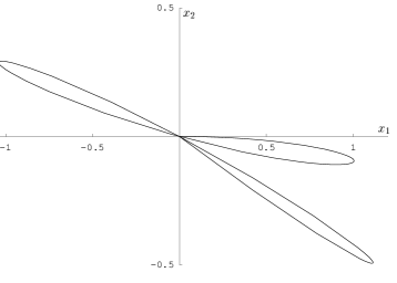
FIG. 1.: Trajectories for $r_{0}=0$ and $v_{0}=\Omega$, after three half-periods for $\kappa=20$, $\gamma=1.2$ and $m=5$. The ratio $\int_{0}^{\tau/2}({\dot{x}}_{1}x_{2}-{\dot{x}}_{2}x_{1})dt/{\cal E}=\pi\frac{\Gamma}{m\Omega^{3}}$ is preserved.

 

Because the physical states $|\psi\rangle$ are periodic ones, let us focus our attention on those. Following [12], one may generally write

$$|\psi(\tau)\rangle = e^{i\phi-\frac{i}{\hbar}\int_{0}^{\tau}\langle\psi(t)|H|\psi(t)\rangle dt}|\psi(0)\rangle$$ (27)

$$= e^{-i2\pi n}|\psi(0)\rangle\,,$$ (28)

i.e. $\frac{\langle\psi(\tau)|H|\psi(\tau)\rangle}{\hbar}\tau-\phi=2\pi n$, $n=0,1,2,\ldots$, which by using $\tau=\frac{2\pi}{\Omega}$ and $\phi=\alpha\pi$, gives

$${\cal H}_{{{}_{I}},e\!f\!f}^{n}\equiv\langle\psi_{n}(\tau)|H|\psi_{n}(\tau)\rangle=\hbar\Omega\left(n+\frac{\alpha}{2}\right)~{},$$ (29)

where the index $n$ has been introduced to exhibit the $n$ dependence of the state and the corresponding energy. ${\cal H}_{{{}_{I}},e\!f\!f}^{n}$ gives the effective $n$th energy level of the physical system, namely the energy given by ${\cal H}_{{{}_{I}}}^{n}$ corrected by its interaction with the environment. We thus see that the dissipation term $J_{2}$ of the Hamiltonian is actually responsible for the “zero point energy” ($n=0$): $E_{0}=\frac{\hbar}{2}\Omega\alpha$.

As well known, the zero point energy is the “signature” of quantization since in Quantum Mechanics it is formally due to the non-zero commutator of the canonically conjugate $q$ and $p$ operators. Thus dissipation manifests itself as “quantization”. In other words, $E_{0}$, which appears as the “quantum contribution” to the spectrum of the conservative evolution of physical states, signals the underlying dissipative dynamics. If we really want to match the Quantum Mechanics zero point energy, we have to resort to experiment, which fixes $\alpha=1$, with $\hbar$ being the Planck constant. In turn this fully exhibits the geometric nature of the phase $\phi$ and gives $R_{0}=\frac{\hbar}{\gamma}$. From Eq.(26) we then see that ${\cal E}_{0}=\frac{1}{2}m\Omega^{2}R_{0}^{2}$ is the energy corresponding to $E_{0}$. We thus put ${\cal E}_{0}=E_{0}$, which gives $\Omega=\frac{\gamma}{m}$, i.e. $\kappa=5\frac{\gamma^{2}}{4m}$, consistent with the reality condition for $\Omega$.

Notice that the only free parameter of the theory is the ratio $\frac{\kappa}{m}$. We also remark that in ref. [4] the phase integral in Eq.(24), which plays there the rôle of dissipative interference phase, has proved to be in fact always non-zero in order to have quantum mechanical interference in the electron double slit experiment. Equivalently, in the present formalism we must always have $x_{1}\neq x_{2}$ (i.e. $r\neq 0$) in order to have $A(t)\neq 0$ (cf. Eq.(19)) and thus a non-zero geometric phase.

In order to better understand the dynamical rôle of $J_{2}$ we rewrite Eq.(16) as follows

$$|\psi(t)\rangle_{H}={\hat{T}}\left[\exp\left(i\frac{1}{\hbar}\int_{u(t_{0})}^{u(t)}2J_{2}du^{\prime}\right)\right]|\psi(t)\rangle_{H_{{}_{I}}}\,,$$ (30)

by using $u(t)=-\Gamma t$. Accordingly, we have

$$-i\hbar\frac{\partial}{\partial u}|\psi(t)\rangle_{H}=2J_{2}|\psi(t)\rangle_{H}\,.$$ (31)

We thus see that $2J_{2}$ is responsible for shifts (translations) in the $u$ variable, as is to be expected since $2J_{2}=p_{u}$ (cf. Eq.(8)). In operatorial notation we can write indeed $p_{u}=-i\hbar\frac{\partial}{\partial u}$. Then, in full generality, Eq.(14) defines families of physical states, representing stable, periodic trajectories (cf. Eq.(15)). $2J_{2}$ implements transition from family to family, according to Eq.(31). Eq.(17) can be then rewritten as

$$i\hbar\frac{d}{dt}|\psi(t)\rangle_{H}=i\hbar\frac{\partial}{\partial t}|\psi(t)\rangle_{H}+i\hbar\frac{du}{dt}\frac{\partial}{\partial u}|\psi(t)\rangle_{H}\,,$$ (32)

where the first term on the r.h.s. denotes of course derivative with respect to the explicit time dependence of the state. The dissipation contribution to the energy is thus described by the “translations” in the $u$ variable. It is then interesting to consider the derivative

$$\frac{\partial S}{\partial U}=\frac{1}{T}\,.$$ (33)

¿From Eq.(9), by using $S\equiv\frac{2J_{2}}{\hbar}$ and $U\equiv 2\Omega{\cal C}$, we obtain $T=\hbar\Gamma$. Eq. (33) is the defining relation for temperature in thermodynamics [13] (with $k_{B}=1$) so that one could formally regard $\hbar\Gamma$ (which dimensionally is an energy) as the temperature, provided the dimensionless quantity $S$ is identified with the entropy. In such a case, the “full Hamiltonian” Eq.(9) plays the rôle of the free energy ${\cal F}$: $H=2\Omega{\cal C}-(\hbar\Gamma)\frac{2J_{2}}{\hbar}=U-TS={\cal F}$. Thus $2\Gamma J_{2}$ represents the heat contribution in $H$ (or $\cal F$). Of course, consistently, $\left.\frac{\partial{\cal F}}{\partial T}\right|_{\Omega}=-\frac{2J_{2}}{\hbar}$. In conclusion $\frac{2J_{2}}{\hbar}$ behaves as the entropy, which is not surprising since it controls the dissipative (thus irreversible) part of the dynamics.

We can also take the derivative of ${\cal F}$ (keeping $T$ fixed) with respect to $\Omega$. We then have

$$\left.\frac{\partial{\cal F}}{\partial\Omega}\right|_{T}=\left.\frac{\partial U}{\partial\Omega}\right|_{T}=mr^{2}\Omega\,,$$ (34)

which is the angular momentum: this is to be expected since it is the conjugate variable of the angular velocity $\Omega$. It is also suggestive that the temperature $\hbar\Gamma$ is actually given by the background zero point energy: $\hbar\Gamma=\frac{\hbar\Omega}{2}$.

In the light of the above results, the condition (14) can be then interpreted as a condition for an adiabatic physical system. $\frac{2J_{2}}{\hbar}$ might be viewed as an analogue of the Kolmogorov–Sinai entropy for chaotic dynamical systems.

Finally, we remark that the thermodynamical picture above outlined is also consistent with the results on the canonical quantization of dissipative system in quantum field theory (QFT) presented in ref. [9]. The transitions between unitarily inequivalent representations of the canonical commutation relations induced by the entropy operator in QFT correspond to the transitions between families of stable trajectories induced by the entropy $\frac{2J_{2}}{\hbar}$ in the present paper.

G.V. is very grateful to Alan Widom for long, illuminating discussions and P.J. wishes to thank John C. Taylor for many useful comments.

REFERENCES

- [1] G. ’t Hooft, Class. Quant. Grav. 16 (1999) 3263.
- [2] G. ’t Hooft, in “Basics and Highlights of Fundamental Physics”, Erice, (1999) [hep-th/0003005].
- [3] G. ’t Hooft, J. Statist. Phys. 53 (1988) 323.
- [4] M. Blasone, Y. N. Srivastava, G. Vitiello and A. Widom, Annals Phys. 267, 61 (1998).
- [5] M. Blasone, E. Graziano, O. K. Pashaev and G. Vitiello, Annals Phys. 252 (1996) 115.
- [6] D. Cangemi, R. Jackiw and B. Zwiebach, Annals Phys. 245, 408 (1996).
- [7] J. S. Bell, “Speakable and unspeakable in Quantum Mechanics.” Cambridge Univ. Pr. (1987).
- [8] T. S. Biro, S. G. Matinian and B. Muller, [hep-th/9908031] ; C. van de Bruck, [gr-qc/0001048].
- [9] E. Celeghini, M. Rasetti and G. Vitiello, Annals Phys. 215 (1992) 156.
- [10] H. Goldstein, “Classical Mechanics”, Addison–Wesley, Reading (1950).
- [11] J. Schwinger, J. Math. Phys. 2 (1961) 407.
- [12] M. V. Berry, Proc. Roy. Soc. Lond. A392, 45 (1984). J. Anandan and Y. Aharonov, Phys. Rev. Lett. 65, 1697 (1990).
- [13] L.D. Landau and E.M. Lifshitz, “ Statistical Physics, Part 1” Pergamon Press, Oxford, (1980).