USITP-00-09
hep-th/0007101 A pedestrian approach to
high energy limits of branes and other gravitational systems

Abstract

In this article we study limits of models that contain a dimensionful parameter such as the mass of the relativistic point-particle. The limits are analogous to the massless limit of the particle and may be thought of as high energy limits. We present the ideas and work through several examples in a (hopefully) pedagogical manner. Along the way we derive several new results.

1 Introduction

The purpose of this article is to give a description and demonstration of methods for deriving high energy limits of various action integrals. It is meant to be readable for a broad range of theoretical physicists, and no expert background is required.

The models we study are described by an action integral of the form $S=T\int dx{\cal L}(\phi,\partial\phi)$, $T$ being some constant and $L=T{\cal L}$ the Lagrangian density. The constant $T$ can typically be neglected at high energy scales, and hence the $T\to 0$ limit may be viewed as a high energy limit. It is this limit which is the focus of this article.

Apart from giving an approximate description of the high energy physics, this limit is also interesting for other reasons. First, it may be that the limit represents a physical situation regardless of the energy scale, in the same sense that photons can be seen as massless particles. Second, the limits typically lead to conformally invariant theories, and one may thus hope to be able to study the original models as broken conformal ones, a point of view which has often proven fruitful.

1.1 Constrained systems

Since one of the methods extensively makes use of the theory for constrained systems, which dates back to Dirac [1], it is useful to briefly review this theory before entering the main subject of this article. A more detailed description is found in e.g. [1, 2, 3].

Suppose you have a Lagrangian density $L$ which depends on some fields $\phi^{i}(x)$ and their derivatives, i.e. $L=L(\phi^{i},\partial_{a}\phi^{i})$, (the index $i$ is not (necessarily) a component index, but used only to keep track of the different fields). Suppose furthermore that you have calculated the canonical conjugate momenta to the fields $\phi^{i}(x)$,

$$\pi^{i}=\frac{\partial L}{\partial\dot{\phi}^{i}}.$$ (1)

Then the naive Hamiltonian is given as usual by

$$H_{naive}=H_{naive}(\phi,\nabla\phi)=\pi_{i}\dot{\phi}^{i}-L(\phi,\partial\phi),$$ (2)

where $\nabla$ signifies spatial derivatives, and $\partial$ signifies all partial derivatives.

In cases where (1) can be inverted to give $\dot{\phi}^{i}=\dot{\phi}^{i}(\phi^{i},\nabla\phi^{i},\pi^{i})$, the naive Hamiltonian can easily be derived just by substitution of $\dot{\phi}^{i}$ as a function of $\pi^{i}$, $\phi^{i}$ and $\nabla\phi^{i}$.

On the other hand, if (1) is not invertible, we have a constrained system. The non-invertibility means that the momenta $\pi^{i}$ will not be independent, and hence that there exist some relations between them. These relations can be expressed as relations $\theta^{I}_{k}(\phi,\pi,\nabla\phi)=0$, $k=1,\dots,M$, where $M$ is the number of independent functions $\theta$. These functions are called the primary constraints (hence the label $I$,) since they follow directly from the definition of the momenta.

Suppose that $i$ can take $N$ different values (i.e. there are $N$ field variables). Then define the $N\times N$ matrix $C_{ij}\equiv\frac{\partial^{2}L}{\partial\dot{\phi}^{i}\partial\dot{\phi}^{j}}$. If $R$ is the rank of this matrix, then the number of independent primary constraints can be shown to be $N-R$.

For constrained systems the naive Hamiltonian is not unique, since any linear combination of the constraint functions $\theta^{I}$ can be added. This fact has implications for Hamilton’s equations, in which the naive Hamiltonian has to be substituted by the extended Hamiltonian

$$H_{I}\equiv H_{naive}+\lambda_{I}^{k}\theta^{I}_{k},$$ (3)

where $\lambda_{I}^{k}$ are coefficients that do not depend on $\phi$ and $\pi$. (No summation over $I$ implied.) These are Lagrange multipliers.

Poisson brackets

Consider two functions $F$ and $G$ that are constructed from $\phi^{i}$ and the conjugate momenta $\pi^{i}$. Writing $F$ as short for $F(\phi(x),\pi(x))$, the Poisson bracket of $F$ and $G$ can be defined by means of functional derivatives as

$$\left\{F,G\right\}\equiv\frac{\delta F}{\delta\phi^{i}}\frac{\delta G}{\delta\pi_{i}}-\frac{\delta F}{\delta\pi_{i}}\frac{\delta G}{\delta\phi^{i}}.$$ (4)

When working with Poisson brackets in the present circumstance the following is important: Poisson brackets must be evaluated before making use of the constraint equations. In other words, calculations should be performed in phase space, and with restriction to the constraint surface ($\theta=0$) only at the very end. To emphasize this point Dirac introduced a notation with a weak equality sign “$\approx$”, and wrote the constraint equations as

$$\theta^{I}_{m}(\phi,\pi)\approx 0.$$ (5)

This makes a difference, for even though $\theta(\phi,\pi)$ is dynamically zero (i.e. zero when $\phi$ and $\pi$ satisfy Hamilton’s equations) it is not zero throughout phase space.

The requirement that the primary constraints should hold at all times, i.e. time derivatives also being weakly zero, leads to a set of consistency conditions $\{\theta^{I}_{m},H_{I}\}\approx 0$, or more explicitly,

$$\{\theta^{I}_{m},H_{naive}\}+\lambda_{I}^{n}\{\theta^{I}_{m},\theta^{I}_{n}\}\approx 0.$$ (6)

This may lead to a set of secondary constraints, $\theta^{II}_{m}\approx 0$, and subsequently, a new set of consistency equations.

When the full constraint structure has been found (i.e. when the consistency conditions do not give anything new), the total Hamiltonian can be written

$$H=H_{naive}+\lambda^{i}\theta_{i},$$ (7)

where $\lambda^{i}$ is a set of independent Lagrange multipliers, and $\theta_{i}$ is the full set of constraints.

1.2 The Naive Hamiltonian for diff invariant models

In this section it is demonstrated that theories which are invariant under diffeomorphisms have a naive Hamiltonian that is dynamically zero, i.e. zero when the field equations are imposed.

A diffeormorphism is a general coordinate transformation of the form

$$x\to\tilde{x}=\tilde{x}(x),$$

where $\tilde{x}(x)$ is a differentiable function of $x$. For models such as the point-particle whose world-line is embedded in spacetime, a world-volume diffeomorphism is often called a reparametrization.

Consider the infinitesimal diffemorphism,

$$x^{a}\to\tilde{x}^{a}=x^{a}+\xi^{a},$$ (8)

which gives the Jacobi determinant

$$J\equiv\det(\frac{\partial x^{b}}{\partial\tilde{x}^{a}})=\det(\delta^{b}_{a}-\partial_{a}\xi^{b})=1-\partial_{a}\xi^{a}+....$$ (9)

Under this change of variables the action integral transforms into

$$S\to\tilde{S}=\int d\tilde{x}L(\tilde{\phi}(\tilde{x}),\tilde{\partial}\tilde{\phi}(\tilde{x}))=\int dx|J^{-1}|L(\tilde{\phi}(\tilde{x}),\tilde{\partial}\tilde{\phi}(\tilde{x})).$$ (10)

Let the transformation of the fields be written in the somewhat unusual form

$$\phi^{i}(x)\to\tilde{\phi}^{i}(\tilde{x})=\phi^{i}(x)+\epsilon^{i}(x).$$ (11)

This defines $\epsilon^{i}$. For scalars this notation will give $\epsilon=0$.

The derivatives of the fields transform as

$$\tilde{\partial}_{b}\tilde{\phi^{i}}(\tilde{x}) = \frac{\partial x^{c}}{\partial\tilde{x}^{b}}\partial_{c}(\phi^{i}(x)+\epsilon^{i})$$ (12)

$$\cong \partial_{b}\phi^{i}(x)+\partial_{b}\epsilon^{i}(x)-\partial_{b}\xi^{c}\partial_{c}\phi(x).$$

The transformed action integral may now be Taylor expanded and rewritten in the following way:

$$\tilde{S} = \int dx(1+\partial_{c}\xi^{c})\left(L(\phi,\partial\phi^{i})+\frac{\partial L}{\partial\phi^{i}}\epsilon^{i}+\frac{\partial L}{\partial(\partial_{a}\phi^{i})}(\partial_{a}\epsilon^{i}-\partial_{a}\xi^{b}\partial_{b}\phi^{i})\right)$$

$$= \int dx\bigg{(}L-\underbrace{\left[\partial_{a}(\frac{\partial L}{\partial(\partial_{a}\phi^{i})})-\frac{\partial L}{\partial\phi^{i}}\right]}_{=\psi_{i}}\epsilon^{i}+\partial_{a}\xi^{b}\underbrace{\left[\delta^{a}_{b}L-\frac{\partial L}{\partial(\partial_{a}\phi^{i})}\partial_{b}\phi^{i}\right]}_{\equiv T^{a}_{~{}b}}\bigg{)}$$

$$= S+\int dx\left(\partial_{a}\xi^{b}T^{a}_{~{}b}-\psi_{i}\epsilon^{i}\right),$$ (13)

where a partial integration has been performed with the assumption that the fields vanish at infinity.

$T^{a}_{~{}b}$ is recognized as the canonical energy-momentum tensor. Of special interest here is the fact that $T^{0}_{~{}0}=-H_{naive}$, by definition. Also, $\psi_{i}=0$ is recognized as the Euler-Lagrange equations.

For diff invariant theories $\delta S=\tilde{S}-S=0$, which gives the condition

$$\int dx\left[T^{a}_{~{}b}\partial_{a}\xi^{b}-\psi_{i}\epsilon^{i}\right]=0.$$ (14)

Consider models made up by tensor fields of zero, first and second rank, i.e. let $\phi^{i}=\{\phi,A_{a},F_{ab}\}$, and define $\Lambda^{b}_{a}\equiv\frac{\partial x^{b}}{\partial\tilde{x}^{a}}=\delta^{b}_{a}-\partial_{a}\xi^{b}$.

For the scalar $\phi$, $\epsilon^{\phi}=0$. For the vector field, $\tilde{A}_{a}(\tilde{x})=\Lambda^{b}_{a}A_{b}(x)=(\delta^{b}_{a}-\partial_{a}\xi^{b})A_{b}(x)$, which gives $\epsilon^{A}_{b}=-\partial_{b}\xi^{a}A_{a}$. For second rank tensors $\tilde{F}_{ab}(\tilde{x})=\Lambda^{c}_{a}\Lambda^{d}_{b}F_{cd}(x)$, which gives $\epsilon^{F}_{ab}=-\partial_{c}\xi^{d}(\delta^{c}_{a}F_{db}+\delta^{c}_{b}F_{ad})$. These contributions add when all fields are present in the Lagrangian.

For actions that depend on scalars, vectors and second rank tensors, the diff symmetry criterion may thus be written

$$\int dx\partial_{a}\xi^{b}\left[T^{a}_{~{}b}+\psi^{a}A_{b}+\psi^{ac}F_{bc}+\psi^{da}F_{db}\right]=0,$$ (15)

where $\psi^{a}$ are the Euler-Lagrange equations associated with $A_{a}$ and $\psi^{ab}$ are the Euler-Lagrange equations associated with $F_{ab}$. This equation should be true for arbitrary $\xi^{a}$, so

$$T^{a}_{~{}b}=-\psi^{a}A_{b}-\psi^{ac}F_{bc}-\psi^{da}F_{db},$$ (16)

and specially

$$H_{naive}=-T^{0}_{~{}0}=\psi^{0}A_{0}+\psi^{0c}F_{0c}+\psi^{d0}F_{d0}$$ (17)

As is well known, the energy-momentum tensor may be modified by terms proportional to the field equations. (It is the Noether current for translations and only conserved on-shell, in general). Hence, with the appropriately redefined energy momentum tensor the corresponding Hamiltonian vanishes. In the terminology introduced in Section (1.1) we may rephrase this as saying that the Hamiltonian is dynamically zero.

The above discussion quantifies a well known result which is only known to us as “folk lore”, except when there are only scalars present, for which case it was proven by von Unge [4]. The above is an adaption of his proof. Our result is not completely general, since only tensor fields have been considered and not, e.g., spinors.

2 Two methods

The starting point is an action of the form

$$S=T\int dx{\cal L}(\phi,\partial\phi),$$ (18)

where $T$ is some constant with dimensions, like mass or string tension. (As mentioned in the introduction, it is a basic assumption that the Lagrangian can be written on this form, $L=T{\cal L}$.) The action (18) is clearly not suitable for studying the $T\to 0$ limit and the philosophy is to search for an action that is classically equivalent to (18) as long as $T\neq 0$, but also well defined for $T=0$. This new action (with $T=0$ inserted) may then be treated as a $T\to 0$ limit of the original model. The two methods presented below are systematic ways for finding such actions. The ideas have been around for quite some time, but we have only been able to find what we believe is the original reference for the second one. (Ref [3])

2.1 Auxiliary field

This is the simplest approach, and involves the introduction of an auxiliary field $\chi$. A reference for this method is [5]. The idea is to define a new action integral,

$$S_{\chi}=\frac{1}{2}\int dx(\chi{\cal L}^{2}+\frac{T^{2}}{\chi}).$$ (19)

This action is equivalent to (18), which can be shown explicitly by solving the equations of motion for $\chi$:

$$\delta\chi\Rightarrow\quad\delta S_{\chi} = \frac{1}{2}\int dx(\delta\chi{\cal L}^{2}-\frac{T^{2}}{\chi^{2}}\delta\chi)$$

$$= \frac{1}{2}\int dx({\cal L}^{2}-\frac{T^{2}}{\chi^{2}})\delta\chi.$$

Using Hamilton’s principle and demanding $\delta S_{\chi}=0$ for arbitrary variations $\delta\chi$ gives

$${\cal L}^{2}-\frac{T^{2}}{\chi^{2}} = 0$$

$$\chi = \frac{T}{{\cal L}};\qquad\mbox{when}\quad T\neq 0.$$ (20)

This expression for $\chi$ substituted back into (19) gives

$$S_{\chi}=\frac{1}{2}\int dx(\frac{T}{{\cal L}}{\cal L}^{2}+\frac{{\cal L}}{T}T^{2})=T\int dx{\cal L}=S.$$

Thus the two actions $S$ and $S_{\chi}$ are equivalent for $T\neq 0$. In addition $S_{\chi}$ allows for the $T\to 0$ limit simply by setting $T=0$ in the action. Doing so gives

$$S_{\chi}^{T=0}=\frac{1}{2}\int dx\chi{\cal L}^{2}.$$ (21)

One natural question is now what this new field $\chi$ really represents. From the current point of view it is impossible to say more than has already been said – that it is useful for the calculations. Hence the name auxiliary field.

Note however, that in the simplest case of a massless particle $\chi$ should be interpreted as the einbein, as will become apparent below.

A general remark on symmetry properties can be made already here. Consider diffeomorphism invariance. The integral measure transforms as $dx\to dxJ^{-1}$, where $J$ is the Jacobi determinant as defined by equation (9). If the original action is to be diff invariant, the Lagrangian must transform as a density, i.e. ${\cal L}\to J{\cal L}$. $S_{\chi}$ is then also diff invariant if $\chi$ transforms as an inverse density (i.e. scalar density of weight $-1$). Since $\chi$ was introduced as an auxiliary field with no a priori physical interpretation, this transformation property is something that can be imposed on $\chi$.

2.1.1 Dynamics

The variation of $\chi$ gives one equation of motion,

$$\delta\chi\Rightarrow\qquad{\cal L}^{2}=0\quad\Rightarrow\quad{\cal L}=0.$$ (22)

The result of a variation in $\phi^{i}$, on the other hand, depends on the form of ${\cal L}$:

$$\delta\phi^{i}\Rightarrow\qquad\delta S = \frac{1}{2}\int dx\chi 2{\cal L}\delta{\cal L}$$

$$= \int dx\chi{\cal L}\left[\frac{\partial{\cal L}}{\partial\phi^{i}}\delta\phi^{i}+\frac{\partial{\cal L}}{\partial(\partial_{a}\phi^{i})}\partial_{a}\delta\phi^{i}\right]$$

$$= \int dx\left[\chi{\cal L}\frac{\partial{\cal L}}{\partial\phi^{i}}-\partial_{a}\left(\chi{\cal L}\frac{\partial{\cal L}}{\partial(\partial_{a}\phi^{i})}\right)\right]\delta\phi^{i}.$$

The field equation is found by demanding $\delta S=0$ for arbitrary $\delta\phi^{i}$. The result is

$$\delta\phi\Rightarrow\qquad\chi{\cal L}\frac{\partial{\cal L}}{\partial\phi^{i}}-\partial_{a}\left(\chi{\cal L}\frac{\partial{\cal L}}{\partial(\partial_{a}\phi^{i})}\right)=0.$$ (23)

Usually, this equation will reduce to an identity by use of equation (22), ${\cal L}=0$. But it does give non-trivial equations in cases where $\frac{\partial{\cal L}}{\partial\phi^{i}}\sim\frac{1}{{\cal L}}$ or $\frac{\partial{\cal L}}{\partial(\partial_{a}\phi^{i})}\sim\frac{1}{{\cal L}}$. (Then the factors ${\cal L}$ are eliminated from equation 23.) This is a special situation, however, and this approach thus has limited applicability.

Generic example: The point particle

The action of a relativistic point particle is

$$S=m\int d\tau\sqrt{-\dot{X}^{\alpha}\dot{X}_{\beta}}=m\int d\tau\sqrt{-\dot{X}^{2}},$$ (24)

where $\dot{X}^{\alpha}\equiv\frac{dX^{\alpha}}{d\tau}$, and $\tau$ is some parametrization of the world-line.

A massless limit can now be found as described above. Introduce the auxiliary field $\chi$ and write

$$S_{\chi} = \frac{1}{2}\int d\tau(\chi{\cal L}^{2}+\frac{m^{2}}{\chi})$$ (25)

$$= \frac{1}{2}\int d\tau(-\chi\dot{X}^{\alpha}\dot{X}_{\alpha}+\frac{m^{2}}{\chi}).$$

This is the manifestly reparametrization invariant form of the point-particle action with $\chi$ acting as the einbein. Putting $m=0$, the reparametrization invariant form of the massless particle results,

$$S_{\chi}^{m=0}=-\frac{1}{2}\int d\tau\chi\dot{X}^{\alpha}\dot{X}_{\alpha}.$$ (26)

2.2 Phase space

This second method of arriving at an action that admits taking the $T\to 0$ limit is designed for constrained systems. Several applications of the method can be found in [3, 5, 6, 7, 8, 9, 10].

Start again with the action (18). Derive the canonical conjugate momenta

$$\pi_{i}=\frac{\partial L}{\partial\dot{\phi^{i}}},$$ (27)

and find the total Hamiltonian as described in Section 1.1,

$$H=H_{naive}+\lambda^{m}\theta_{m}.$$ (28)

The derivation of the total Hamiltonian $H$ involves working out the constraint structure, which can be a cumbersome task.

Having found the total Hamiltonian, the phase space action is:

$$S^{PS}=\int dx\left(\pi_{i}\dot{\phi^{i}}-H(\phi,\pi,\nabla\phi)\right).$$ (29)

The momenta $\pi_{i}$ can then be eliminated by solving their equations of motion. Substituting for the solutions of $\pi_{i}$ gives a new configuration space action

$$S^{CS}=\int dx\left[\pi(\phi,\partial\phi)\dot{\phi}-H(\phi,\pi(\phi,\partial\phi),\nabla\phi)\right].$$ (30)

Unless the system under study is un-constrained (giving $H=H_{naive}$) this action will contain new variables (the Lagrange multipliers) compared to the original action (18). In other words, it is different from the original configuration space action, but still equivalent to it (see figure 1).

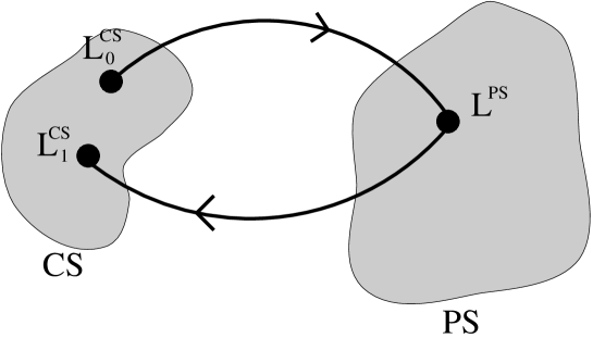
Figure 1: Start with a Lagrangian $L^{CS}_{0}$ in configuration space (CS), and perform a Legendre transform to the phase space (PS) Lagrangian $L^{PS}$. Going back to configuration space may, for constrained systems, give a new (but equivalent) Lagrangian $L^{CS}_{1}\neq L^{CS}_{0}$. And although $L^{CS}_{0}$ is not defined in the limit $T=0$, $L^{PS}$ or $L^{CS}_{1}$ may be.

In some cases (such as the point particle) this new form makes it possible to take the $T\to 0$ limit, but in general the merit of this approach is that one may take the limit at the level of constraints.

When there are no constraints the above construction will be circular and give back the original action. However, it may still be possible to make sense of the $T\to 0$ limit in the intermediate phase space description. This is illustrated in some of the applications in Section 3 below.

Again, the generic example which illustrates the method is provided by the point particle.

The point particle

From the action (24) one finds the momenta,

$$P_{\alpha}=\frac{\partial L}{\partial\dot{X}^{\alpha}}=-\frac{m\dot{X}_{\alpha}}{\sqrt{-\dot{X}^{2}}}.$$ (31)

The naive Hamiltonian vanishes since

$$H_{naive}=P_{\alpha}\dot{X}^{\alpha}-L=0.$$ (32)

This is in accordance with the diff invariance of the action integral (24) and the discussion in section 1.2

The expression for $P_{\alpha}$ is not invertible, leading to one primary constraint,

$$\theta=P^{2}+m^{2}\approx 0,$$ (33)

where $P^{2}\equiv P^{\alpha}P_{\alpha}$. There are no secondary constraints, and the total Hamiltonian is $H=\lambda(P^{2}+m^{2})$, which gives the following phase space action:

$$S^{PS}=\int d\tau\left(P_{\alpha}\dot{X}^{\alpha}-\lambda(P^{\alpha}P_{\alpha}+m^{2})\right).$$ (34)

A variation in $P_{\alpha}$ gives

$$\delta P_{\alpha}\Rightarrow\qquad\delta S^{PS}=\int d\tau(\dot{X}^{\alpha}-2\lambda P^{\alpha})\delta P_{\alpha},$$ (35)

which by use of Hamilton’s principle leads to a solution for the momentum,

$$P^{\alpha}=\frac{\dot{X}^{\alpha}}{2\lambda}.$$ (36)

Substituted back into (34) this gives a new configuration space action,

$$S^{CS}=\frac{1}{2}\int d\tau\left(\frac{1}{2\lambda}\dot{X}^{\alpha}\dot{X}_{\alpha}-2m^{2}\lambda\right).$$ (37)

A comparison with the result (25) found by method I reveals that the two methods give exactly the same result, with the identification $\chi=(-2\lambda)^{-1}$.

3 Applications

Both these methods have been applied to a variety of models before, and to get an overview and further references, the reader may consult [6]. In the subsequent sections of this article the methods are applied to Weyl-invariant strings, D-strings, and to general relativity. Many of the results are known and included as illustrations, but, e.g., the applications to the manifestly diffeomorphism invariant actions (43), (60) and (73) below, are new.

3.1 The Bosonic string

The Nambu Goto string

The Nambu-Goto form of the action for a bosonic string is [11, 12]

$$S=T\int d^{2}\xi\sqrt{-\gamma},$$ (38)

where $\xi^{a}$ parameterizes the world sheet, $\gamma\equiv\det(\gamma_{ab})$, and $\gamma_{ab}$ is the induced metric, $\gamma_{ab}\equiv G_{\alpha\beta}\frac{\partial X^{\alpha}}{\partial\xi^{a}}\frac{\partial X^{\beta}}{\partial\xi^{b}}=G_{\alpha\beta}\partial_{a}X^{\alpha}\partial_{b}X^{\beta}$, $G_{\alpha\beta}$ being the spacetime metric.

In [13, 5] it is shown that in the tensionless limit $T\to 0$ the Nambu-Goto string gives a spacetime conformally invariant theory with a degenerate metric, a so-called null string. Only the results are presented here.

The auxiliary field method gives the action

$$S=-\frac{1}{2}\int d^{2}\xi~{}\chi\gamma,$$ (39)

where $\chi$ is an auxiliary field.

The phase space method leads to a Hamiltonian which can be written

$$H=\lambda(P^{2}+T^{2}\acute{X}^{2})+\rho P_{\alpha}\acute{X}^{\alpha},$$ (40)

where $\dot{X}^{\alpha}\equiv\frac{\partial X^{\alpha}}{\partial\xi^{0}}$, and $\acute{X}^{\alpha}\equiv\frac{\partial X^{\alpha}}{\partial\xi^{1}}$, and $\lambda$ and $\rho$ are Lagrange multipliers. Integrating out the momenta from the corresponding phase space action and recombining the Lagrange multipliers into a metric yields the manifestly reparametrization invariant form (43) below. Taking the limit $T\to 0$ in (40) and repeating the procedure yields

$$S_{1} = \int d^{2}\xi~{}V^{a}V^{b}\gamma_{ab},$$ (41)

where the Lagrange multipliers have been combined into the vector density $V^{a}$ instead. If one chooses to also integrate out one of the lagrange multipiliers, the result is

$$S_{2} = \frac{1}{2}\int d^{2}\xi~{}\frac{\gamma}{V},$$ (42)

where $V$ is a scalar density. With the appropriate identification this is again (39). Interpretations of the last two actions are given e.g. in [7].

The “Polyakov form”

A Weyl-invariant form of the string action that is equivalent to the Nambu Goto action was found by Brink, Di Vecchia and Howe [14], and by Deser and Zumino [15] It was used by Polyakov to study quantum properties of strings and is usually referred to as the Polyakov action. It reads

$$S=\frac{T}{2}\int d^{2}\xi\sqrt{-g}g^{ab}\gamma_{ab},$$ (43)

where $g_{ab}$ is an auxiliary metric, and $g\equiv\det(g_{ab})$, and the Weyl invariance means that the action is invariant under rescalings $g_{ab}\to\Omega g_{ab}$ of the metric.

The auxiliary field method becomes difficult to use for this form of the action, although by making use of the Weyl-invariance one can indeed show that the resulting equations are equivalent to those of (41) and (42). This is left as an edifying exercise for the ambitious reader.

Phase space

Before applying the phase space method to the action (43) a few remarks are needed.

First, when viewed in the “center of momentum” frame where $P_{\alpha}=(E,\underline{0})$, the limit $m\to 0$ in (33), or $T\to 0$ in (40) is equivalent to neglecting the rest-mass or tension, respectively, compared to the energy $E$. (This is why the limits discussed may be labelled “high energy limits”). Formally, then, the limits may be achieved by neglecting terms proportional to $m$ or $T$ compared to those proportional to the momentum $P$.

Second, in the manifestly reparametization invariant formulation of the theory, there is no longer a clear separation into, e.g., $T$-dependent and $T$-independent terms. Therefore a new approach is needed.

In view of these remarks, the strategy to be adopted is to rescale to dimensionless fields and then ignore terms independent of $P$. This gives an unambigous way of finding the limit of large momenta.

Rescaling $X^{\alpha}\to\sqrt{T}X^{\alpha}$, the action (43) becomes

$$S=\frac{1}{2}\int d^{2}\xi\sqrt{-g}g^{ab}\gamma_{ab},$$ (44)

The momenta are:

$$P_{\alpha} \equiv \frac{\partial L}{\partial\dot{X}^{\alpha}}=\sqrt{-g}(g^{00}\dot{X}_{\alpha}+g^{10}\acute{X}_{\alpha}).$$ (45)

In addition, the momenta $\Pi^{ab}$ for the auxiliary metric $g_{ab}$ vanishes everywhere. This is consistent with the phase space derivation where the metric arose as a combination of Lagrange multipliers. It is safe to ignore its momentum constraint and time-derivative in the construction of the Hamiltonian. Unlike the cases previously discussed, (45) is nondegenerate and may be solved for $\dot{X}^{\alpha}$:

$$\dot{X}_{\alpha}=\frac{1}{g^{00}}\left(\frac{P_{\alpha}}{T\sqrt{-g}}-g^{10}\acute{X}_{\alpha}\right).$$ (46)

The fact that this is possible further means that the momenta are independent functions of $\dot{X}^{\alpha}$. Thus there are no constraints in the theory.

The Hamiltonian now follows directly. In absence of constraints the total Hamiltonian equals the naive Hamiltonian.

$$H = P_{\alpha}\dot{X}^{\alpha}-L$$

$$= P_{\alpha}\dot{X}^{\alpha}-\frac{1}{2}\sqrt{-g}(g^{00}\dot{X}^{\alpha}\dot{X}_{\alpha}+2g^{01}\dot{X}^{\alpha}\acute{X}_{\alpha}+g^{11}\acute{X}^{\alpha}\acute{X}_{\alpha})$$

$$= \frac{1}{2g^{00}\sqrt{-g}}(P^{2}+\acute{X}^{2})-\frac{g^{01}}{g^{00}}P\cdot\acute{X}.$$

Dropping the term independent of $P$ (the term $\propto\acute{X}^{2}$) and integrating out the momenta from the phase space action yields

$$S=2\int d^{2}\xi\left[{(g^{01})^{2}}\over{g^{00}}\acute{X}^{2}+2g^{01}\dot{X}\cdot\acute{X}+g^{00}\dot{X}^{2}\right].$$ (47)

The action (47) is nolonger reparametrization invariant with $g^{00}$ and $g^{01}$ transforming as components of a second rank tensor. However, making the field redefinitions

$$V^{0}\equiv\sqrt{2\over{g^{00}}}(-g)^{\frac{1}{4}}g^{01},\qquad V^{1}\equiv\sqrt{2g^{00}}(-g)^{\frac{1}{4}},$$ (48)

we recover the reparametrization invariant action (41) in terms of the vector density $V^{a}$. This illustrates how unconstrained models may be handled.

3.2 The D-string

D-branes are extended objects that arise naturally in string theory. They are defined by the property that open strings can end on them, but have their own dynamics. A D-string is another name for a D1-brane i.e. a 2-dimensional D-brane.

The fluctuations of the D-string is described by the Dirac-Born-Infeld (DBI) action, so called because of its similarities to the Dirac action for membranes and to the Born-Infeld action [16]. Disregarding the dilaton field, it is [17]

$$S=T\int d^{2}\xi~{}\sqrt{-\det(\gamma_{ab}+B_{ab}+F_{ab})},$$ (49)

where $T\equiv\frac{1}{2g\pi\alpha^{\prime}}$ is a constant, $g$ is the string coupling and $2\pi\alpha^{\prime}$ is the inverse of the fundamental string tension, and $F_{ab}=2\pi\alpha^{\prime}\partial_{[a}A_{b]}$, $A_{a}$ being an abelian gauge field. Furthermore,

$$\gamma_{ab}(\xi)\equiv\partial_{a}X^{\alpha}\partial_{b}X^{\beta}G_{\alpha\beta}(X);\qquad B_{ab}(\xi)\equiv\partial_{a}X^{\alpha}\partial_{b}X^{\beta}{\cal B}_{\alpha\beta}(X)$$ (50)

are the induced metric and antisymmetric tensor pulled back to the brane. $G_{\alpha\beta}$ is the background (symmetric) metric, and ${\cal B}_{\alpha\beta}$ is the background (antisymmetric) Kalb-Ramond field. (Hitherto $G$ has been taken to be constant and ${\cal B}$ to vanish in the discussion of strings.)

Because of the relation between $T$ and $g$ the $T\to 0$ limit may be viewed as a strong coupling limit where $g\to\infty$ and $\alpha^{\prime}$ is held fixed.

The independent fields in this action are the embedding $X^{\alpha}(\xi)$ and the gauge fields $A_{a}(\xi)$. If $A_{a}=0$ the D-string reduces to the bosonic string.

The DBI action

Defining $M_{ab}\equiv\gamma_{ab}+B_{ab}+F_{ab}$, the tensionless limit found using an auxiliary field is easily seen to be

$$S^{T=0}_{\chi}=-\frac{1}{2}\int d^{p+1}\xi~{}\chi\det(M_{ab}).$$ (51)

The equation of motion for $\chi$ is found from a variation $\delta\chi$:

$$\delta\chi\Rightarrow\quad\det(M_{ab})=0.$$ (52)

This is similar to what was found for the bosonic string. But in the present case the degeneracy does not imply that the world volume is a null surface. It merely gives a relation between the $X^{\alpha}$ and $A_{a}$ fields.

The phase space approach described in [18] gives a Hamiltonian

$$H=P^{a}\partial_{a}A_{0}+\lambda\Theta_{A}+\rho^{i}\Theta_{i}+\sigma\Theta_{B}+\tau\Theta_{C},$$ (53)

where $P^{a}$ is the canonical conjugate momentum to $A_{a}$, and $\lambda$, $\rho$, $\sigma$, and $\tau$ are Lagrange multipliers, and (with ${\cal B}_{\alpha\beta}$ set to zero)

$$\Theta_{1} \equiv \Pi_{\alpha}\partial_{1}X^{\alpha}+\frac{P^{1}}{2\pi\alpha^{\prime}}F_{11}\approx 0,$$ (54)

$$\Theta_{A} \equiv \Pi_{\alpha}\Pi^{\alpha}+\frac{P^{1}\gamma_{11}P^{1}}{(2\pi\alpha^{\prime})^{2}}+T^{2}\det(M_{11})\approx 0,$$ (55)

$$\Theta_{B} \equiv P^{0}\approx 0,$$ (56)

$$\Theta_{C} \equiv \partial_{c}P^{c}\approx 0,$$ (57)

are the constraints, with $\Pi_{\alpha}$ the conjuagate momentum to $X^{\alpha}$.

Integrating out the momenta from the phase space action and redefining fields in terms of the Lagrange multipliers gives a manifestly diffeomorphism invariant form of (49), just as for the ordinary string. The resulting action is given in (60) below.

Taking the $T\to 0$ limit in (53) and repeating the procedure results in the tensionless limit of the DBI-string:

$$S_{2}^{T=0}=\frac{1}{4}\int d^{p+1}\xi V^{a}W^{b}M_{ab},$$ (58)

where $V^{a}$ and $W^{a}$ are the new vector density fields defined from the Lagrange multipliers. Integrating out one of the Lagrange multipliers in addition to the momenta yields

$$S_{1}^{T=0} = \frac{1}{4}\int d^{p+1}\xi V\det(M_{ab}),$$ (59)

where $V$ is a scalar density. The result would essentially be the same with the background field ${\cal B}_{\alpha\beta}$ included. The second action (59) is identical to what was found in (51). The action (58) can be shown [18] to imply that the world surface of the D-string generally splits into a collection of tensile strings or, in special cases, massless particles. Thus it leads to a parton picture of D-branes in this limit.

The Weyl-invariant form

An equivalent, but Weyl-invariant form of the D-string action was constructed in [19]

$$S=\frac{T}{2}\int d^{2}\xi\sqrt{-s}s^{ab}M_{ab},$$ (60)

where $s\equiv\det(s_{ab})$ and $s_{ab}$ is an auxiliary tensor field with no symmetry assumed. Elimination of $s_{ab}$ gives the DBI action (49).

Phase space

The $T\to 0$ limit of the action (60) can only be meaningfully discussed in the phase space approach. As discussed immediately before equation (44), the starting point should be the action (60) with the fields rescaled to be dimensionless. In this case a convenient rescaling is $X^{\alpha}\to\sqrt{T}X^{\alpha}$ and $A_{a}\to 2\pi\alpha^{\prime}TA_{a}$. Instead of doing this, the discussion below shows that the Hamiltonian can be brought to the same form as that of the DBI action, equation (53). The subsequent limit $T\to 0$ will then be the same. The fields to be considered as independent variables in the action (60) are $X^{\alpha}$, $A_{a}$ and $s_{ab}$. Setting ${\cal B}_{\alpha\beta}=0$, the canonical conjugate momenta for these fields are.

$$\Pi_{\alpha} \equiv \frac{\partial L}{\partial\dot{X}^{\alpha}}=T\sqrt{-s}\left(s^{00}\dot{X}_{\alpha}+\frac{1}{2}(s^{01}+s^{10})X_{\alpha}^{\prime}\right)$$ (61)

$$P^{a} \equiv \frac{\partial L}{\partial\dot{A}_{a}}=T\sqrt{-s}\frac{1}{2}(s^{0a}-s^{a0})2\pi\alpha^{\prime}$$ (62)

$$\Sigma^{ab} \equiv \frac{\partial L}{\partial\dot{s}_{ab}}=0$$ (63)

The first equation (61) is invertible which means that an explicit expression for $\dot{X}^{\alpha}$ can be obtained:

$$\dot{X}_{\alpha}=\frac{1}{s^{00}}\left(\frac{\Pi_{\alpha}}{T\sqrt{-s}}-\frac{1}{2}(s^{01}+s^{10})X_{\alpha}^{\prime}\right)$$ (64)

The second equation (62) is obviously not invertible since the momentum $P$ is completely independent of the fields $A$. Its definition results in the following constraints

$$\Theta_{0} \equiv P^{0}\approx 0,$$ (65)

$$\Theta_{1} \equiv P^{1}-\frac{T}{2}\sqrt{-s}(s^{01}-s^{10})2\pi\alpha^{\prime}\approx 0.$$ (66)

The last equation (63) says that the conjugate momenta to $s_{ab}$ are identically zero. This reflects the fact that $s_{ab}$ are non-dynamical variables to be treated on the same footing as Lagrange multipliers (cf. the comment following (45)).

Now, derive the naive Hamiltonian. Disregarding $\Sigma^{ab}$,

$$H_{naive} = \Pi_{\alpha}\dot{X}^{\alpha}+P^{a}\dot{A}_{a}-\frac{T}{2}\sqrt{-s}s^{ab}(\gamma_{ab}+2\pi\alpha^{\prime}(\partial_{a}A_{b}-\partial_{b}A_{a})).$$

Some rearrangements yield a simpler form,

$$H_{naive} = \frac{1}{2Ts^{00}\sqrt{-s}}\left(\Pi_{\alpha}\Pi^{\alpha}+\frac{P^{1}\gamma_{11}P^{1}}{(2\pi\alpha^{\prime})^{2}}+T^{2}\gamma_{11}\right)$$ (67)

$$-\frac{s^{01}+s^{10}}{2s^{00}}\Pi_{\alpha}X^{\prime\alpha}+P^{a}\partial_{a}A_{0}.$$

The consistency condition on the primary constraint $\Theta_{0}$ gives a secondary “Gauss law” constraint

$$\Theta_{2}\equiv\partial_{a}P^{a}\approx 0,$$ (68)

while $\Theta_{1}$ gives nothing new. There are no tertiary constraints. The four component fields of $s_{ab}$ are Lagrange multipliers which can be redefined as

$$\lambda \equiv \frac{1}{2Ts^{00}\sqrt{-s}},$$ (69)

$$\rho \equiv -\frac{s^{01}+s^{10}}{2s^{00}},$$ (70)

$$\varphi \equiv \frac{T}{2}\sqrt{-s}(s^{01}-s^{10}).$$ (71)

Including the constraints, the total Hamiltonian is obtained and reads

$$H = \lambda(\Pi^{2}+\frac{P^{1}\gamma_{11}P^{1}}{(2\pi\alpha^{\prime})^{2}}+T^{2}\gamma_{11})+\rho\Pi_{\alpha}\partial_{1}X^{\alpha}+P^{a}\partial_{a}A_{0}$$ (72)

$$+\sigma_{0}P^{0}+\sigma_{1}(P^{1}+\varphi)+\tau\partial_{a}P^{a}$$

The phase space Lagrangian is $L^{PS}=\Pi_{\alpha}\partial_{0}X^{\alpha}+P^{a}\partial_{0}A_{a}-H$, and a variation of $\varphi$ gives $\sigma_{1}=0$, which means that the constraint $\Theta_{1}=P^{1}+\varphi$ in fact makes no difference. Then it is obvious that this is exactly the same Hamiltonian and phase space Lagrangian as was found from the DBI action for the D-string (53).

A rescaled version of the above expressions is achieved by putting $T=1$, and the limit $T\to 0$ is then equivalent to dropping terms that do not contain the momenta. The exact procedure follows from the discussion in [18] and results in the actions (58) and (59), as mentioned above.

The treatment of the Weyl-invariant $D$-string parallels that of the Polyakov string versus the Nambu-Goto string. This is no surprise, since the string action can be seen as a special case of the D-string action where $A_{a}={\cal B}_{\alpha\beta}=0$, and $s_{ab}$ is symmetric.

3.3 General relativity

The Hilbert action describing the dynamics of spacetime is

$$S[g]=\frac{1}{\kappa}\int d^{4}x\sqrt{-g}g^{\alpha\beta}R_{\alpha\beta},$$ (73)

where $\kappa$ is a constant, $g\equiv\det(g_{\alpha\beta})$, $g_{\alpha\beta}$ is the metric, and $R_{\alpha\beta}$ is the Ricci tensor (a function of the metric and its first and second derivatives). The limit to be studied in this case is $\kappa\to\infty$. Einstein’s constant $\kappa$ is defined as $\kappa\equiv\frac{8\pi}{c^{3}}G_{N}$, so this limit can be thought of as either a limit where Newton’s gravitational constant $G_{N}\to\infty$ or a limit where the speed of light $c\to 0$. As the speed of light approaches zero, lightcones will collapse into spacetime lines, and points in space become disconnected. So this limit leads to an ultralocal field theory.

Yet another interpretation of this limit comes from the observation (which is possible in the Hamilton formulation) that it is equal to the zero signature limit, which represents some intermediate stage between Euclidean space (signature $+1$) and Minkowski space (signature $-1$) [22].

Although the action above in appearance very much resembles the Polyakov string action (43), it is considerably more intricate to analyze. Nevertheless the limit can be found using the phase space approach in suitable coordinates.

Phase space

A fruitful approach to a Hamiltonian description of general relativity is the ADM approach [20]. The crucial step is the introduction of a new set of variables, replacing the 10 independent components of the metric $g_{\alpha\beta}$. The new variables are the lapse function $N$, the shift functions $N_{\mu}$, and the 3-dimensional induced metric (on a hypersurface $\Sigma$) $h_{\mu\nu}$, with the following relation to the four dimensional metric:

$$g_{\alpha\beta}=\left(\begin{array}[]{cc}N_{\mu}N^{\mu}-N^{2}&N_{\nu}\\ N_{\mu}^{T}&h_{\mu\nu}\end{array}\right);\qquad\begin{array}[]{l}\alpha,\beta=0,1,2,3;\\ \mu,\nu=1,2,3.\end{array}$$ (74)

Through some reformulations, and the derivations of the canonical conjugate momenta, the Hamiltonian is found to be

$$H=\tilde{N}\theta+N_{\nu}\theta^{\nu},$$ (75)

where $\tilde{N}\equiv\kappa N$, and $\theta$ and $\theta^{\nu}$ are to be considered as constraints,

$$\theta = \frac{1}{\sqrt{h}}(\pi^{\mu\nu}\pi_{\mu\nu}-\frac{1}{2}\pi^{2})-\frac{1}{\kappa^{2}}\sqrt{h}R_{\Sigma},$$ (76)

$$\theta^{\nu} = -2D_{\mu}\pi^{\mu\nu}.$$ (77)

Here, $\pi^{\mu\nu}$ is the canonical conjugate momentum to $h_{\mu\nu}$, $R_{\Sigma}$ is the Ricci scalar on the hypersurface $\Sigma$ and $D_{\mu}$ is the covariant derivative on $\Sigma$.

Taking the limit $\kappa\to\infty$ is now possible by just dropping the last term in $\theta$. (Note that if we rescale to dimensionless coordinates in (73) this again amounts to dropping terms not containing momenta.) And as mentioned above, this has the same effect as taking the zero signature limit $\varepsilon\to 0$. The signature $\varepsilon$ of the spacetime metric only influences this term, and enters in such a way that taking $\varepsilon\to 0$ removes the term proportional to $\sqrt{h}R$ [21].

This limit has in turn been shown [22] to correspond to the four-dimensional action

$$S=\int d^{4}x\Omega(x)({\cal K}^{\alpha\beta}{\cal K}_{\alpha\beta}-{\cal K}^{2});\quad\alpha,\beta=0,1,2,3.$$ (78)

The equivalence can be demonstrated by showing that this action gives the same Hamilton formulation (75) as the $\varepsilon\to 0$ limit of the general relativity action.

The independent fields in the action (78) are the positive scalar density $\Omega(x)$ and the components of a symmetric covariant tensor $\tilde{g}_{\alpha\beta}(x)$. This “metric” $\tilde{g}_{\alpha\beta}$ is degenerate, i.e. $\det(\tilde{g}_{\alpha\beta})=0$, which means that it has at most 9 independent components. Together with $\Omega$ this gives 10 independent fields, which is the same number as in the original action.

${\cal K}_{\alpha\beta}$ is the second fundamental tensor, defined as the Lie derivative in a unique direction $\vec{e}$,

$${\cal K}_{\alpha\beta}=\frac{1}{2}\pounds_{e}\tilde{g}_{\alpha\beta}=\frac{1}{2}(e^{\gamma}\tilde{g}_{\alpha\beta,\gamma}+e^{\gamma}_{,\alpha}\tilde{g}_{\gamma\beta}+e^{\gamma}_{,\beta}\tilde{g}_{\alpha\gamma}).$$ (79)

And the vector field $\vec{e}$ is defined through

$${\cal G}^{\alpha\beta}=\Omega^{2}e^{\alpha}e^{\beta};\qquad{\cal G}^{\alpha\beta}\equiv\frac{1}{3!}\varepsilon^{\alpha\gamma\delta\epsilon}\varepsilon^{\beta\zeta\eta\theta}\tilde{g}_{\gamma\zeta}\tilde{g}_{\delta\eta}\tilde{g}_{\epsilon\theta}.$$ (80)

Hence ${\cal G}^{\alpha\beta}$ is the minor of $\tilde{g}_{\alpha\beta}$. The vector $\vec{e}$ is completely determined from $\tilde{g}_{\alpha\beta}$ and $\Omega$. It satisfies $\tilde{g}_{\alpha\beta}e^{\beta}=0$ and is thus orthogonal to any other vector $v^{\alpha}$, i.e. $\tilde{g}_{\alpha\beta}e^{\alpha}v^{\beta}=0$.

Since the metric is degenerate (i.e. the determinant vanishes), there is no inverse $\tilde{g}^{\alpha\beta}$ satisfying $\tilde{g}^{\alpha\beta}\tilde{g}_{\beta\gamma}=\delta^{\alpha}_{\gamma}$. However, the class of symmetric tensors $G^{\alpha\beta}$ defined by

$$G^{\alpha\beta}\tilde{g}_{\beta\gamma}=\delta^{\alpha}_{\gamma}-\Theta_{\gamma}e^{\alpha},$$ (81)

where $\Theta_{\gamma}$ is an arbitrary vector satisfying $\Theta_{\gamma}e^{\gamma}=1$, may instead be used to raise indices which makes ${\cal K}=G^{\alpha\beta}{\cal K}_{\alpha\beta}$ and ${\cal K}^{\alpha\beta}{\cal K}_{\alpha\beta}$ well defined.

For an elaboration of the ideas presented above, the reader should consult [22].

The result of this section is that it is possible to find an interesting limit using the phase space method. This is not as straight forward as in the string cases, but by introduction of the more suitable ADM coordinates, it can be done.

The most troublesome part is the step from phase space to configuration space. This can not be easily done by integrating out momenta and redefining the Lagrange multipliers as before. Instead, the idea is to make an ansatz for a configuration space action, and then to show that it gives the right Hamiltonian.

As for the string models, it was found that the limit corresponds to a degenerate geometry. In the present case, this means a non-Riemannian space halfway between Euclidean and Minkowski space, which corresponds to a theory of gravity based, not on local Poincaré invariance, but on local Caroll invariance.

4 Conclusions

One aim of this article was to present methods for deriving tensionless limits of strings and the analogue in other models. This has been done by giving a general description as well as several explicit calculations.

An interesting result that was given in the introduction is the derivation of the naive Hamiltonian for diffeomorphism invariant theories with only tensor fields. It was demonstrated that for such models the Hamiltonian is constrained to be zero when the fields satisfy the field equations.

A second goal of the article has been to investigate the applicability of the methods. It was known from before that they work well for a number of string models. The derivations here has revealed that the methods work perfectly also if we start from the Weyl-invariant form of the bosonic string and D-string actions. These are models that already at the very beginning contain Lagrange multipliers (an auxiliary metric). The methods apply in such cases as well, which emphasizes their generality.

Applying the methods to General Relativity turned out not to be quite straight forward. However, by changing to ADM coordinates, the phase space treatment yielded expressions that could be handled.

A general remark is that in the tensionless limit, the string models provide conformally invariant theories, and that the geometries turn out to be degenerate. That the point particle action has spacetime conformal symmetry is well known. This result is directly generalizable to the other brane-actions discussed and is explicitly shown in the cited literature on the $T\to 0$ limit. The same holds for the degeneracy. A massless point particle moves on a null geodesic, a tensionless string moves on a null-surface. The induced metric is thus degenerate as is the metric in the $\kappa\to\infty$ limit of General relativity.

Acknowledgement

We thank Björn Brinne and Rikard von Unge for comments. The work of U L was supported in part by a grant from the Swedish Natural Sciences Research Council, and by “The European Superstring Theory Network”, part of the EU program for Training and Mobility of Researchers (TMR). H G S gratefully acknowleges support from the Nordic Council of Ministers in the form of a Nordplus grant.

Notation

The spacetime dimension is denoted $D$, and the world-volume dimension is denoted $d$. (For particles $d=1$, and for strings $d=2$.) To refer to components of world-volume variables, small Latin indices are used: From the beginning of the alphabet for general components, and middle alphabet letters when only spatial components are referred to, i.e. $a,b=0,\dots,d-1$; $m,n=1,\dots,d-1$.

Spacetime variables are denoted by Greek indices in the same way,$\alpha,\beta=0,\dots,D-1$; $\mu,\nu=1,\dots,D-1$.

References

- [1] P A M Dirac. Lecture notes on quantum mechanics. In Belfer graduate school of science, Monograph series. Yeshiva University, 1964.
- [2] M Henneaux and C Teitelboim. Quantization of Gauge Systems. Princeton University Press, 1992.
- [3] R Marnelius. Introduction to the quantization of general gauge theories. Acta Phys.Pol., B13:669–690, 1982.
- [4] R von Unge. Classes of classical -branes and quantization of the conformal string. Lic-thesis at Fysikum, University of Stockholm, e-print: http://vanosf.physto.se/licavh/licavh.html, 1994.
- [5] A Karlhede and U Lindström. The classical bosonic string in the zero tension limit. Class.Quant.Grav., 3:L73–75, 1986.
- [6] J Isberg, U Lindström, B Sundborg, and G Theodoridis. Classical and quantized tensionless strings. Nucl.Phys., B411:122–156, 1994.
- [7] U Lindström, B Sundborg, and G Theodoridis. The zero tension limit of the superstring. Phys.Lett., B253:319–323, 1991.
- [8] U Lindström, B Sundborg, and G Theodoridis. Phys.Lett., B258:331, 1991.
- [9] U Lindström and M Roček. Phys.Lett., B271:79, 1991.
- [10] S Hassani, U Lindström, and R von Unge. Classically equivalent actions for tensionless -branes. Class.Quant.Grav., 11:L79–85, 1994.
- [11] Y Nambu. Duality and hydrodynamics. Lectures at the Copenhagen symposium, 1970.
- [12] T Goto. Prog.Theor.Phys., 46:1560, 1971.
- [13] A Schild. Classical null strings. Phys.Rev., D16:1722–1726, 1977.
- [14] L Brink, P Di Vecchia, and P Howe. A locally supersymmetric and reparametrization invariant action for the spinning string. Phys.Lett., 65B:471–474, 1976.
- [15] S Deser and B Zumino. A complete action for the spinning string. Phys.Lett., 65B:369–373, 1976.
- [16] M Born and L Infeld. Proc.Roy.Soc., A144:425, 1934.
- [17] J Polchinski. String theory. Cambridge University Press, 1998.
- [18] U Lindström and R von Unge. A picture of D-branes at strong coupling. Phys.Lett., B403:233, 1997.
- [19] U Lindström. First order actions for gravitational systems, strings and membranes. Int.J.Mod.Phys., A3:2401–2416, 1988.
- [20] R Arnowitt, S Deser, and C W Misner. The dynamics of general relativity. In L Witten, editor, Gravitation: an introduction to current research. John Wiley & Sons, 1982.
- [21] C Teitelboim. Proper time approach to the quantization of the gravitational field. Phys.Lett., 96B:77, 1980.
- [22] M Henneaux. Zero Hamiltonian signature spacetimes. Bull.Soc.Math.Belg., 31:47, 1979.