S-Duality, Noncritical Open String

and

Noncommutative Gauge Theory  

Soo-Jong Rey^a and Rikard von Unge^b

School of Physics & Center for Theoretical Physics

Seoul National University, Seoul 151-742 Korea ^a

Department of Theoretical Physics & Astrophysics

Masaryk University, Brno CZ-61197 Czech Republic ^b

abstract

We examine several aspects of S-duality of four-dimensional noncommutative gauge theory. By making duality transformation explicit, we find that S-dual of noncommutative gauge theory is defined in terms of dual noncommutative deformation. In ‘magnetic’ noncommutative U(1) gauge theory, we show that, in addition to gauge bosons, open D-strings constitute important low-energy excitations: noncritical open D-strings. Upon S-duality, they are mapped to noncritical open F-strings. We propose that, in dual ‘electric’ noncommutative U(1) gauge theory, the latters are identified with gauge-invariant, open Wilson lines. We argue that the open Wilson lines are chiral due to underlying parity noninvariance and obey spacetime uncertainty relation. We finally argue that, at high energy-momentum limit, the ‘electric’ noncommutative gauge theory describes correctly dynamics of delocalized multiple F-strings.

1 Introduction

Following the recent understanding concerning the equivalence between non-commutative and commutative gauge theories [1], an immediate question to ask is how the theory behaves under the S-duality interchanging the strong and weak coupling regimes. Indeed, this question has been addressed in several recent works [2, 3, 4, 5, 6] (See also related works [7, 8, 9, 10, 11, 12]).

One expects an answer as simple as follows. The four-dimensional non-commutative theory describes the low-energy worldvolume dynamics of a D3-brane in the presence of a background of NS-NS two-form potential (Kalb-Ramond potential) $B_{2}$ but none others. Under the S-duality of the Type IIB string theory, the D3-brane is self-dual, while the NS-NS two-form potential $B_{2}$ is swapped with the R-R two-form potential $C_{2}$. Thus, after the S-duality, the dual theory appears to be the one describing the low-energy worldvolume dynamics of a D3-brane in the presence of a R-R two-form potential $C_{2}$, but none others. Since there is no NS-NS two-form potential present, noncommutative deformation via Seiberg-Witten map is not possible and the resulting theory ought to be a commutative theory. However, this is apparently not the answer one obtains [3, 4, 6]. Starting with a noncommutative U(1) gauge theory with coupling constant $g$ and noncommutativity tensor $\theta$ and taking the standard duality transformation, one finds that the dual theory still remains a noncommutative U(1) gauge theory, but with coupling and noncommutativity parameters

$$g_{\rm D}={1\over g}\qquad{\rm and}\qquad\theta_{\rm D}=-g^{2}\widetilde{\theta},$$ (1)

where $\widetilde{\theta}^{\mu\nu}={1\over 2}{\epsilon^{\mu\nu}}_{\alpha\beta}\theta^{\alpha\beta}$. Alternatively, as is done in [3, 4], one may utilize the gauge invariance of $(F+B_{2})$ to dial out the space-space noncommutativity and treat the theory as the standard gauge theory in a constant magnetic field. The S-duality would then turn this into a dual gauge theory, but now in a constant electric field, which is gauge equivalent to a theory with space-time noncommutativity. Actually, in the dual theory, it turns out to be impossible to take a field theory limit that the dual theory would be best described by a noncritical open string theory, whose tension is of the order of the noncommutativity scale.

The aim of this paper is to understand the S-duality via the following routes:

$$\begin{array}[]{ccc}{\rm D3-brane}&\longleftrightarrow&\widetilde{\rm D3}-{\rm brane}\\ \uparrow&&\uparrow\\ |&&|\\ |&&|\\ \downarrow&&\downarrow\\ {\rm NCYM}&\longleftrightarrow&\widetilde{\rm NCYM}\\ \end{array}$$ (8)

and, if possible, to reconcile these seemingly different results concerning the S-duality of the noncommutative gauge theory from various perspectives.

2 Naive S-Duality

In this section, we shall be studying S-duality of noncommutative U(1) gauge theory . The latter is defined by the following action:

$$S = {1\over 4g^{2}}\int\!d^{4}x\,\mbox{Tr}\Big{(}{\cal F}\star{\cal F}\Big{)},$$ (9)

where the noncommutative field strength is defined by

$${\cal F}=\bf F+i\{A_{\mu},A_{\nu}\}_{\star},\qquad\bf F_{\mu\nu}=(\partial_{\mu}A_{\nu}-\partial_{\nu}A_{\mu})$$

and Tr refers to “matrix notation” for spacetime index contractions, for instance, $\mbox{Tr}\left({\cal F}{\cal F}\right)$ means ${{\cal F}_{\mu}}^{\nu}{{\cal F}_{\nu}}^{\mu}$. Seiberg and Witten have found explicitly the map between ${\cal F}_{\mu\nu}$ and $\bf F_{\mu\nu}$ :

$${\cal F}=\bf F-\left[\bf F\theta\bf F-(A\theta\partial)\bf F\right]+\cdots.$$ (10)

The map Eq.(10) allows to expand the action Eq.(9) in powers of dimensionless combination $\theta\bf F$:

$$S=\frac{1}{4g^{2}}\int d^{4}x\,\left[-\mbox{Tr}\left(\bf F\bf F\right)+2\mbox{Tr}\left(\theta\bf F\bf F\bf F\right)-\frac{1}{2}\mbox{Tr}\left(\theta\bf F\right)\mbox{Tr}\left(\bf F\bf F\right)+\cdots\right].$$ (11)

Adopting the standard rule of duality transformation, we can promote the field strength $\bf F$ (not ${\cal F}$) into an unconstrained field by including a term $\widetilde{\bf G}\bf F$ where $\widetilde{\bf G}_{\mu\nu}=\frac{1}{2}\epsilon_{\mu\nu}^{\;\;\;\;\rho\sigma}\bf G_{\rho\sigma}$ and $\bf G_{\mu\nu}=\partial_{\mu}B_{\nu}-\partial_{\nu}B_{\mu}$. Varying with respect to $\bf B$ imposes the constraint $d{\bf F}=0$ which is solved by ${\bf F}=d{\bf A}$ and we get back the original theory. On the other hand we can now vary with respect to $\bf F$ which gives us

$$g^{2}\widetilde{\bf G}={\bf F}-(\theta{\bf F}{\bf F}+{\bf F}\theta{\bf F}+{\bf F}{\bf F}\theta)+\frac{1}{4}\mbox{Tr}\left({\bf F}{\bf F}\right)\theta+\frac{1}{2}\mbox{Tr}\left(\theta{\bf F}\right){\bf F}+\cdots$$

which can be inverted, to the lowest order in $\theta$, as

$${\bf F}=g^{2}\widetilde{\bf G}+g^{4}\theta\widetilde{\bf G}\widetilde{\bf G}+g^{4}\widetilde{\bf G}\theta\widetilde{\bf G}+g^{4}\widetilde{\bf G}\widetilde{\bf G}\theta-\frac{g^{4}}{4}\mbox{Tr}\left(\widetilde{\bf G}\widetilde{\bf G}\right)\theta-\frac{g^{4}}{2}\mbox{Tr}\left(\theta\widetilde{\bf G}\right)\widetilde{\bf G}+\cdots.$$

After the duality transformation, the action becomes

$$S=\frac{g^{2}}{4}\int\!d^{4}x\,\left[\mbox{Tr}\left(\widetilde{\bf G}\widetilde{\bf G}\right)+2g^{2}\mbox{Tr}\left(\theta\widetilde{\bf G}\widetilde{\bf G}\widetilde{\bf G}\right)-\frac{g^{2}}{2}\mbox{Tr}\left(\theta\widetilde{\bf G}\right)\mbox{Tr}\left(\widetilde{\bf G}\widetilde{\bf G}\right)+\cdots\right].$$

This can be rewritten as

$$S=\frac{1}{4g_{\rm D}^{2}}\int\!d^{4}x\,\left[-\mbox{Tr}\left(\bf G\bf G\right)+2\mbox{Tr}\left(\theta_{D}\bf G\bf G\bf G\right)-\frac{1}{2}\mbox{Tr}\left(\theta_{D}\bf G\right)\mbox{Tr}\left(\bf G\bf G\right)+\cdots\right],$$ (12)

where $g_{\rm D}$ and $\theta_{\rm D}$ are given as in Eq.(1). It is evident that the above action can be reorganized into a self-dual form

$$S=\frac{1}{4g_{\rm D}^{2}}\int\!d^{4}x\,\mbox{Tr}\Big{(}{\cal G}\widetilde{\star}{\cal G}\Big{)}$$ (13)

when expanded in powers of $\theta_{\rm D}{\bf G}$ and expressed noncommutativity via $\theta_{\rm D}$, where

$${\cal G}_{\mu\nu}=\bf G_{\mu\nu}+i\{B_{\mu},B_{\nu}\}_{\widetilde{\star}},\qquad\bf G_{\mu\nu}=\partial_{\mu}{\bf B}_{\nu}-\partial_{\nu}{\bf B}_{\mu}.$$

Thus, we find that the dual action Eq.(13) is again noncommutative U(1) gauge theory, but with dual coupling parameters Eq.(1). Note here that if we started with a theory with space-space non-commutativity, the dual theory will have space-time non-commutativity.

The foregoing analysis may be extended to the situation where R-R zero-form $C$ and two-form $C_{2}$ background is turned on. In this case, the full action takes the form:

$$S_{\rm total}=S+\int\!d^{4}x\,\left[\frac{1}{2}C\mbox{Tr}\left(\bf F\widetilde{\bf F}\right)+\mbox{Tr}\left({\bf F}\widetilde{C}_{2}\right)+\cdots\right].$$

Here, one may wonder what form of the coupling one ought to use. One could for instance imagine that the correct coupling should be given by a standard form but in terms of the noncommutative field strength, for example, $C\mbox{Tr}\left({\cal F}\star{\widetilde{\cal F}}\right)$, etc. We have checked, again to the lowest order in noncommutativity parameter, that modifying the coupling in this fashion does not change the final result we will draw.

It is obvious that the effect of the R-R two-form potential is simply to shift ${\bf G}\rightarrow{\bf G}+C_{2}$ everywhere and, for the R-R zero-form, a straightforward calculation shows that the action is self-dual (i.e. of the same form as the original one) under the duality transformation provided that we define the dual parameters and backgrounds as:

$$g_{D}^{-2} = \frac{g^{-2}}{\left(g^{-4}+C^{2}\right)}$$

$$C_{D} = -\frac{C}{\left(g^{-4}+C^{2}\right)}$$ (14)

$$\theta_{D} = C_{D}\theta-\frac{1}{g_{D}^{2}}\tilde{\theta}.$$

These are the results anticipated from Type IIB S-duality:

$${\rm S}_{\rm IIB}:\qquad\quad\left(C+{i\over g^{2}}\right) \rightarrow -\left(C+{i\over g^{2}}\right)^{-1}$$

$$\left(\theta+i\widetilde{\theta}\right) \rightarrow \left(C+{i\over g^{2}}\right)^{-1}\left(\theta+i\widetilde{\theta}\right).$$ (15)

Note that, had we started with an original theory having purely ‘electric’ or ‘magnetic’ noncommutativity, viz. $\theta$ is a tensor of rank-1, in the presence of the R-R scalar background, the dual theory would have noncommutativity tensor $\theta_{\rm D}$ of full rank.

3 Closer Look - Noncritical Open String

We have seen, in the previous section, that the naive S-dual of a noncommutative gauge theory is again a noncommutative gauge theory, but with the noncommutativity parameter $\theta_{\rm D}=-g^{2}\tilde{\theta}$. Thus, if the original theory were defined with ‘magnetic’ noncommutativity, the dual theory would have ‘electric’ noncommutativity and vice versa. We also note that, in performing the S-duality map, as we have expanded the original and the dual actions as in Eq.(11) and Eq.(12), respectively, the result would be valid only for $\theta{\bf F}\ll 1$ and $\theta_{\rm D}{\bf G}\ll 1$. The latter requires that $g\ll 1$ and, in this case, the physics in the original and the dual theories wouldn’t be different much from the standard commutative gauge theories .

What can one say for the $g\gg 1$ case, viz. the original theory is strongly coupled? In order to understand this limit, for definiteness, we will take the noncommutativity purely ‘magnetic’: $\theta=\theta_{23}$. The spectrum in this theory includes, in addition to the U(1) gauge boson, the magnetic monopole and the dyon (See [13] and references therein). They may be viewed as noncommutative deformations of the photon, the magnetic monopoles and the dyons in the standard U(1) gauge theory. In noncommutative gauge theory, the U(1) gauge boson can be visualized as an induced electric dipole.

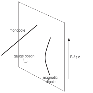
Figure 1: Cartoon view of gauge boson (open F-string dipole), Dirac magnetic monopole and magnetic dipole (open D-string dipole).

Alternatively, one may analyze the spectrum as fundamental (F-) or D-strings, respectively, ending on the D3-brane on which background magnetic field is turned on. The latter should be describable in terms of the Dirac-Born-Infeld Lagrangian ($T_{\rm F}=1/2\pi\alpha^{\prime}$):

$$L_{\rm DBI}=-{T_{\rm F}^{2}\over\lambda_{\rm st}}\sqrt{-g_{00}g_{11}}\sqrt{g_{22}g_{33}+{\bf F}_{23}^{2}/T_{\rm F}^{2}}$$

where, in the Seiberg-Witten decoupling limit, the bulk coupling parameter are related to the gauge theory parameters in Eq.(9) as

$$\lambda_{\rm st}={g^{2}\over T_{\rm F}\theta},\qquad-g_{00}=g_{11}=1,\qquad g_{22}=g_{33}=\left({1\over T_{\rm F}\theta}\right)^{2},\qquad{\bf F}_{23}=\left({1\over\theta}\right)\epsilon_{23}.$$

The magnetic monopoles are not part of the physical spectrum as, being represented by semi-infinite D-string ending on the D3-brane, they are counterpart of the Dirac magnetic monopole with an infinite self-energy. Among the physical excitations, however, are magnetic dipoles (as well as their dyonic counterparts) composed of monopole-antimonopole pair. See figure 1. Consider an open D-string (lying entirely on the D3-brane) of length $\Delta{\bf x}$. It represents a magnetic dipole carrying a dipole moment ${\bf m}=\Delta{\bf x}$ (measured in string unit) and total mass

$$M_{\rm dipole}=\left({T_{\rm F}\over\lambda_{\rm st}}\right)|\Delta{\bf x}|-{\bf m}\cdot{\bf H}.$$ (16)

where the negative sign in the second term refers to relative opposite orientation between the dipole and the background magnetic field. The last term represents the interaction energy of the magnetic dipole with the background magnetic field:

$${\bf H}=-{\partial L_{\rm DBI}\over\partial{\bf F}_{23}}={\bf H}_{\rm c}\left[1+\left({1\over T_{\rm F}\theta}\right)^{2}\right]^{-1/2},$$ (17)

where ${\bf H}_{\rm c}$ denotes the critical magnetic field strength

$${\bf H}_{\rm c}={T_{\rm F}\over\lambda_{\rm st}}.$$

In the field theory limit $T_{\rm F}\rightarrow\infty$, the magnetic dipole remain as low-energy excitaitons – they are noncritical open D-strings with an effective tension

$$T_{\rm eff}={M_{\rm dipole}\over|\Delta{\bf x}|}\quad\longrightarrow\quad{1\over 2g^{2}\theta}.$$ (18)

In Eq.(16), the negative sign in the second term refers to relative opposite orientation between the dipole and the background magnetic field. It implies that the noncritical open D-string representing the magnetic dipole ought to be chiral: open D-string with opposite orientation, which represents magnetic anti-dipole, is separated by an infinite mass gap from the magnetic dipoles. Thus, from the open D-string point of view, the field theory limit $T_{\rm F}\rightarrow\infty$ amounts to taking non-relativistic limit and allows to expand Eq.(17) in power-series of $(1/T_{\rm F}\theta)^{2}$. This also account for physical origin of the numerical factor 1/2 in Eq.(18) .

Taking the strong coupling limit, $g\gg 1$, unlike the magnetic monopoles, the magnetic dipoles are nearly tensionless, weakly interacting degrees of freedom, while the U(1) gauge bosons are tensionless, strongly interacting degrees of freedom. Performing S-duality Eq.(1) to the dual gauge theory, the two are interchanged with each other: the dual electric dipoles are nearly tensionless, weakly interacting degrees of freedom and the dual magnetic dipoles are tensionless but strongly interacting degrees of freedom. They are made out of open F- and D-strings ending on the dual D3-brane worldvolume, on which a background dual electric field ${\bf G}_{01}$ is turned on. The background dual electric field ought to be near critical, as is anticipated from S-duality and evidenced by the fact that, for fixed $\theta$, $\theta_{\rm D}=g^{2}\theta$ becomes infinitely large. Indeed, combining the S-duality transformation of gauge theory parameters Eq.(1) and of bulk coupling parameters

$$\lambda_{\rm D,st}={1\over\lambda}_{\rm st}\qquad{\rm and}\qquad g_{\rm D,\mu\nu}={1\over\lambda}_{\rm st}g_{\mu\nu},$$

we find that ${\bf F}_{23}$ is mapped to displacement field ${\bf D}=-({\partial L_{\rm DBI}/\partial{\bf G}_{01}})$ and the dual electric field ${\bf E}_{\rm D}:={\bf G}_{01}$ is given by

$${\bf E}_{\rm D}={\bf E}_{\rm c}\left[1+\left({1\over g_{\rm D}^{2}T_{\rm F}\theta_{\rm D}}\right)^{2}\right]^{-1/2}\qquad{\rm where}\qquad{\bf E}_{\rm c}=g^{4}_{\rm D}T_{\rm F}^{2}\theta_{\rm D}.$$

Likewise, magnetic dipoles are mapped into electric dipoles made out of open F-strings, whose effective tension is given by the S-dual of Eq.(18):

$$\widetilde{T}_{\rm eff}={1\over 2\theta_{\rm D}},$$ (19)

where again the factor of 1/2 ought to signify chiral nature of the open F-string. An immediate question is: are these nearly tensionless, open F-strings identifiable within the dual gauge theory?

A set of gauge invariant operators in the dual gauge theory is given by the following open Wilson lines [15]:

$$\widetilde{W}_{\bf k}[C]=\int\!d^{2}{\bf x}\,\exp_{\widetilde{\star}}\Big{[}i\int_{C}\,\dot{y}(t)\cdot{\bf B}(x+y(t))\Big{]}\,\widetilde{\star}\,e^{i{\bf k}\cdot{\bf x}}.$$ (20)

Here, $t=[0,1]$ denotes the affine parameter along the open Wilson line, $x^{\mu}$ refers to the spacetime position of the $\tau=0$ point, ${\bf x}$ to the projection of $x^{\mu}$ onto the two-dimensional noncommutative spacetime and ${\bf k}$ to the Fourier-momentum along the noncommutative spacetime. All the multiplications are defined in terms of the ‘generalized Moyal product’:

$$A(x)\,\widetilde{\star}\,B(y)\,\,:=\,\,\exp\left({i\over 2}\theta^{\mu\nu}_{\rm D}\partial_{\mu}^{x}\partial_{\nu}^{y}\right)A(x)B(y).$$

It is then straightforward to check that the Wilson line Eq.(20) is gauge invariant provided the following relation holds between the momentum ${\bf k}_{\mu}$ and the endpoint separation distance:

$${\bf k}_{\mu}=\left({1\over\theta_{\rm D}}\right)_{\mu\nu}\Delta y^{\nu}\qquad\,\,\,{\rm where}\qquad\,\,\,\Delta y\equiv y(1)-y(0).$$ (21)

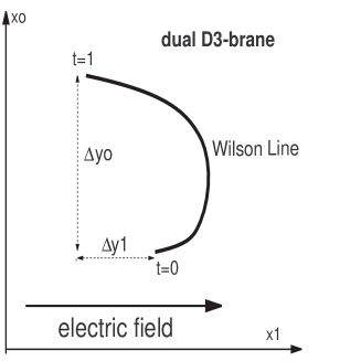
Figure 2: Characteristic shape of Wilson line.

What happens here is that, once the relation Eq.(21), the extra phase factor $e^{i{\bf k}\cdot{\bf x}}$ effectively parallel transports the gauge transformation parameter at $t=1$ back to that at $t=0$. This then ensures that the noncommutative Wilson line, despite being an open string, is gauge invariant. Being so, much as the closed Wilson loops form a complete set of gauge invariant observables in Yang-Mills theory, we can take the noncommutative Wilson lines Eq.(20) as a complete set of gauge invariant observables of the dual noncommutative U(1) gauge theory .

For small total energy or momentum, $|{\bf k}|\ll 1/\sqrt{\theta_{\rm D}}$, separation between the Wilson line endpoints is shorter than the non-commutativity scale, $|\Delta y|\ll\sqrt{\theta_{\rm D}}$. Hence, the Wilson line reduces effectively to a (Fourier-transform) of the standard closed Wilson loop. For energies smaller than the non-commutativity scale $1/{\sqrt{\theta_{\rm D}}}$, we would expect the dual theory behaves as in the standard gauge theory. This agrees with the conclusions of [3, 4, 6]. On the other hand, if $|{\bf k}|\gg 1/\sqrt{\theta_{\rm D}}$, then the separation of the Wilson line endpoints would be larger than the noncommutativity scale, $|\Delta y|\gg\sqrt{\theta_{\rm D}}$. These excitations are string-like.

Taking the zeroth component of Eq.(21), one finds

$$E_{\rm YM}\,\,:=\,\,\widetilde{T}_{\rm eff}\,\Delta y^{1},$$ (22)

where $\widetilde{T}_{\rm eff}$ coincides precisely with the effective tension Eq.(19). Thus, we are prompted to identify the Wilson line with a noncritical open F-string, whose effective tension is given by $\widetilde{T}_{\rm eff}$. Recall that, under the S-duality Eq.(1), $T_{\rm eff}=1/2g^{2}\theta$ is mapped to $\widetilde{T}_{\rm eff}=1/2\theta_{\rm D}$. Hence, the open Wilson lines in the dual gauge theory are the right candidates for the S-dual of the magnetic dipoles in the original gauge theory.

Characteristic size of the open Wilson lines is ${\cal O}(\sqrt{\theta_{\rm D}})$ and become macroscopically large in the strong coupling limit $g\gg 1$. They represent a complete set of excitations in the weakly coupled, dual gauge theory for $|{\bf k}|\geq 1/\sqrt{\theta_{\rm D}}\sim 0$. It clearly suggests that the noncommutative gauge theory captures more of the description than we had the right to expect from the naive duality argument in Section 2. It also indicates that a suitable formulation of the dual gauge theory is in terms of macroscopic open strings.

In extracting tension of the open Wilson line from Eq.(22), we were able to match it to Eq.(19) modulo a numerical factor of 2. Recall that the numerical factor of 1/2 in Eqs.(18, 19) has originated from chiral or, equivalently, non-relativistic nature of the open D- and F-strings. What then would cause the open Wilson lines of the noncommutative Yang-Mills theory chiral and eventually account for cancellation or disappearance of the factor of 2 in Eq. (22)?

We believe an answer to this question comes from the fact that ‘electric’ noncommutative Yang-Mills theory is parity-violating. For fixed $\theta_{\rm D}$, this is easily seen from non-invariance of the electric noncommutativity $[x^{0},x^{1}]=\theta_{\rm D}$ under ${\bf x}\rightarrow-{\bf x}$ . This then implies that, along the $(x^{0}-x^{1})$-directions along which ${\bf k}_{\mu}$ and $\Delta y^{\mu}$ in Eq.(21) point, the open Wilson lines ought to be chiral, stretching the two endpoints such that $\Delta y^{1}$ positive. This chirality also implies that, from Eq.(22), only positive energy Wilson lines are physical excitations but not negative energy ones. The net result is essentially the same as that of the infinite mass gap opening up in the non-relativistic limit.

There exists one more piece of evidence that the Wilson lines are indeed identifiable with a sort of macroscopic string. Utilizing $E\sim\Delta E\geq\hbar/\Delta y^{0}$, we observe that the Wilson line exhibits a version of the spacetime uncertainty relation:

$$\Delta y^{0}\Delta y^{1}\,\,\geq\,\,{1\over 2}\hbar\theta_{\rm D}.$$

As emphasized by Yoneya [17], the spacetime uncertainty relation is a distinguishing feature of any string theory with worldsheet conformal invariance.

4 Yet Another Look – Strong Noncommutativity Limit

We would like to discuss yet another piece of physics associated with the S-duality, Eq.(1). In the previous section, we have seen that, due to the dual electric field background, the open F-string is oriented predominantly along the $x^{0}-x^{1}$ directions. See Eq.(21). There, we have also argued that the open string is macroscopically stretched. According to Eq.(20), the open string is made out of the dual gauge field ${\bf B}_{\mu}$ as a sort of coherent state configuration. Thus, it ought to be possible to visualize the open string out of the dual gauge theory in the semiclassical limit. In this section, under suitable condition, we show that the dual gauge theory Eq.(13) describes worldsheet dynamics of $N_{\rm F}$ coincident macroscopic F-strings propagating in four dimensional spacetime.

Let us begin with the following elementary observation. Strongly coupled noncommutative U(1) gauge theory with a finite noncommutativity $\theta$, as is seen from Eq.(1), is dual to weakly coupled noncommutative U(1) gauge theory with an infinite noncommutativity $\theta_{\rm D}$. In dimensionless measure, this implies that

$$\theta_{\rm D}\{{\bf B}_{\mu},{\bf B}_{\nu}\}\,\,\sim\,\,\theta_{\rm D}\big{(}\partial{\bf B}\big{)}\,\,\gg\,\,1$$ (23)

and hence corresponds to high field-strength, high-energy limit . Because of the infinitely large noncommutativity, dynamics of the dual ‘electric’ U(1) gauge theory is considerably simplified. At leading order in the noncommutativity Eq.(23), the dual gauge theory action Eq.(13) is reduced as:

$$S\quad\rightarrow\quad{1\over 4g_{\rm D}^{2}}V_{\perp}\int dx^{0}dx^{1}\Big{<}\,\,\left({\cal G}_{\mu\nu}\right)^{2}_{\widetilde{\star}}\,\,\Big{>},$$

where the Lorentz indices are contracted with gauge theory metric. We have also introduced notations

$$V_{\perp}\equiv\int dx^{2}dx^{3}\qquad{\rm and}\qquad\Big{<}\,\,{\cal O}\,\,\Big{>}\equiv{1\over V_{\perp}}\int dx^{2}dx^{3}{\cal O}.$$ (24)

In the limit of infinitely many coincident noncommutative D3-branes, it is known that nonabelian generalization of the dual gauge theory Eq.(13) may be interpreted as a theory describing low-energy dynamics of (F1-D3) bound states [16, 4, 19]. It is known that, in this case, the Yang-Mills gauge coupling is not arbitrary but is determined by the F-string and the D3-brane charges $N_{\rm F},N_{\rm D3}$ [19]:

$$g_{\rm D}^{2}={V_{\perp}\over\theta_{\rm D}}\left({N_{\rm D3}\over N_{\rm F}}\right).$$

Thus, using this parameter relation and introducing new covariant operator variables

$$X^{\mu}=\theta^{\mu\nu}_{\rm D}\left(i\partial_{\nu}+{\bf B}_{\nu}\right),$$

we can re-express the dual ‘electric’ noncommutative Yang-Mills theory action as:

$$S=-{N_{\rm F}T_{\rm eff}\over 2}\int dx^{0}dx^{1}\left(-{1\over 2}\left<\,\,\left({1\over\theta_{\rm D}}\{X^{\mu},X^{\nu}\}_{\widetilde{\star}}\right)^{2}\,\,\right>+\cdots\right)$$ (25)

where again the Lorentz indices are contracted with respect to the gauge theory metric and the ellipses denote ${\cal O}(1)$ sub-leading terms. We have thus found that the resulting action Eq.(25) has precisely the same form as string worldsheet action for $N_{\rm F}$ multiple noncritical, F-strings of tension $T_{\rm eff}$, except that the action is expressed in the so-called Schild gauge [20]. The F-strings ought to be interpreted as open strings, albeit infinitely stretched, as they propagate in a spacetime governed by the gauge theory metric. Note that the worldsheet direction is along $(x^{0}-x^{1})$-directions and the strings are delocalized along $(x^{2}-x^{3})$-directions.

Actually, what we have gotten is not precisely the Schild-gauge action but a deformation quantization of it. Namely, plaquette element $\Sigma^{\mu\nu}$ of the string worldsheet is deformed into

$$\Sigma^{\mu\nu}\equiv\epsilon^{ab}\partial_{a}X^{\mu}\partial_{b}X^{\nu}=\{X^{\mu},X^{\nu}\}_{\rm PB}\qquad\rightarrow\qquad\Sigma^{\mu\nu}_{\widetilde{\star}}\equiv{1\over\theta_{\rm D}}\{X^{\mu},X^{\nu}\}_{\widetilde{\star}}.$$ (26)

We trust the deformation is correctly normalized, as $\Sigma^{\mu\nu}_{\widetilde{\star}}=\Sigma^{\mu\nu}+{\cal O}(\theta_{D})$ in small $\theta_{\rm D}$ limit.

What conclusion can one draw out of the above result? Had we considered $N_{3}$ coincident D3-branes with $N_{\rm F}$ units of center-of-mass U(1) electric flux turned on, we would have obtained the standard Nambu-Goto or Schild action of $N_{\rm F}$ F-strings. Recalling that noncommutative U(1) gauge theory is equivalent to $\rm U(\infty)$ gauge theory at high-energy regime, we may interpret that the dual ‘electric’ noncommutative gauge theory indeed describes worldsheet dynamics of $N_{\rm F}$ coincident F-strings provided the latter carry high energy-momentum and become open strings (see Eq.(21)), and are delocalized along $(x^{2}-x^{3})$-directions. The result seems consistent with what one finds from supergravity dual [4, 19].

Acknowledgement

We thank M.R. Douglas, J. Klusoň, U. Lindström and G. Moore for useful discussions. SJR thanks warm hospitality of Marsaryk University, New High-Energy Theory Center at Rutgers University, and Theory Division at CERN during completion of the work.

References

- [1] N. Seiberg and E. Witten, J. High-Energy Phys. 9909 (1999) 032, hep-th/9908142.
- [2] S.-J. Rey and R. von Unge, unpublished work (December, 1999).
- [3] N. Seiberg, L. Susskind and N. Toumbas, J. High-Energy Phys. 0006 (2000) 021, hep-th/0005040.
- [4] R. Gopakumar, J. Maldacena, S. Minwalla and A. Strominger, S-Duality and Noncommutative Gauge Theory, hep-th/0005048.
- [5] O. J. Ganor, G. Rajesh and S. Sethi, Duality and Non-Commutative Gauge Theory, hep-th/0005046.
- [6] S. J. Rey, Open String Dynamics with Nonlocality in Time, to appear, SNUST-00605.
- [7] J.L.F. Barbon and E. Rabinovici, Phys. Lett. B486 (2000) 202, hep-th/0005073.
- [8] J. Gomis and T. Mehen, Nucl. Phys. B591 (2000) 265, hep-th/0005129.
- [9] R. Gopakumar, S. Minwalla, N. Seiberg and A. Strominger, J. High-Energy Phys. 0008 (2000) 008, hep-th/0006062.
- [10] J.G. Russo and M.M. Sheikh-Jabbari, J. High-Energy Phys. 0007 (2000) 052, hep-th/00006202.
- [11] L. Alvarez-Gaume and J.L.F. Barbon , Nonlinear Vacuum Phenomena in Noncommutative QED, hep-th/0006209.
- [12] T. Kawano and T. Terashima, S-Duality from OM Theory, hep-th/0006225.
- [13] D.J. Gross and N.A. Nekrasov, J. High-Energy Phys. 0007 (2000) 034, hep-th/0005204.
- [14] I.R. Klebanov and J. Maldacena, 1+1 Dimensional NCOS and Its U(N) Gauge Theory, hep-th/0006085.
-
[15]
N. Ishibashi, S. Iso, H. Kawai and Y. Kitazawa,
Nucl. Phys. B573 (2000) 573, hep-th/9910004;
S.R. Das and S.-J. Rey, Nucl. Phys. B590(2000) 453, hep-th/0008042;
D.J. Gross, A. Hashimoto and N. Itzhaki, Observables of Noncommutative Gauge Theories, hep-th/0008075. - [16] N. Ishibashi, Nucl. Phys. B539 (1999) 107; A Relation between Commutative and Noncommutative Descriptions of D-Branes, hep-th/9909176; J.-X. Lu and S. Roy, Nucl. Phys. B579 (2000) 229.
- [17] T. Yoneya, String Theory and the Space-Time Uncertainty Principle, hep-th/0004074.
- [18] R. Gopakumar, S. Minwalla and A. Strominger, J. High-Energy Phys. 0005 (2000) 020.
-
[19]
, T. Harmark, J. High-Energy Phys. 0006 (2000) 043,
hep-th/0006023;
J.X. Lu, S. Roy and H. Singh, J. High-Energy Phys. 0009 (2000) 020, hep-th/0006193. - [20] A. Schild, Phys. Rev. D16 (1977) 1722.