NTUA-95/00

hep–th/0007079

Lattice Evidence for Gauge Field Localization on a Brane

P. Dimopoulos, K. Farakos, A. Kehagias and G. Koutsoumbas Physics Dept., National Technical Univ.,
Zografou Campus, 157 80 Athens, Greece

Abstract

We examine the problem of gauge-field localization in higher-dimensional gauge theories. In particular, we study a five-dimensional $U(1)$ by lattice techniques and we find that gauge fields can indeed be localized. Two models are considered. The first one has anisotropic couplings independent of each other and of the coordinates. It can be realized on a homogeneous but anisotropic flat Euclidean space. The second model has couplings depending on the extra transverse fifth direction. This model can be realized by a $U(1)$ gauge theory on the Randall-Sundrum background. We find that in both models a new phase exists, the layer phase, in which a massless photon is localized on the four-dimensional layers. We find that this phase is separated from the strong coupling phase by a second order phase transition.

July 2000

1 Introduction

The idea that we live in a higher-dimensional space-time is not new. The general setting is a $(4+n)$-dimensional space-time with $n$ dimensions compactified and the vacuum is of the form $M^{1,3}\!\times\!X^{n}$. $M^{1,3}$ is the four-dimensional Minkowski space-time we experience and $X^{n}$ is an internal compact space. The compactness of the internal space is crucial since the four-dimensional Planck mass $M_{Pl}$ is related to the $4+n$ dimensional Planck mass $M_{(4+n)}$ by $M_{Pl}^{2}=M_{(4+n)}^{2+n}V_{n}$ where $V_{n}$ is the volume of $X^{n}$. It is exactly this relation which allows for a large volume internal space [1],[2]. Thus, as we see, four-dimensional gravity exists as long as the volume of the internal space is finite. The latter requirement together with the smoothness of the internal space can be satisfied with a compact space $X^{n}$. Non-compact internal spaces have also been considered in the past at the cost of giving up smoothness [3],[4],[5],[6],[7]. Indeed, all such cases are suffering from naked singularities. However, there are also cases where such singularities are not that bad as for example delta-function singularities to which a physical interpretation may be given as domain walls, strings, etc. This is the case in the Randall-Sundrum (RS) model, where the singularities may be interpreted as a four-dimensional domain wall, a three-brane, embedded in a five dimensional bulk [8]. In that case, although the internal space may be non-compact, a four-dimensional graviton exists and it is localized at the three-brane. The question one would like to answer is if in this case, localization on the 3-brane exists for other fields, like gauge fields, fermions and scalars.

It is known that solitons like domain walls or strings, may support massless fields. In theories with domain walls formed by a scalar field (vortex field) for example, scalars as well as fermions with appropriate interactions in the bulk give rise to massless scalars and chiral fermions on the wall [9]–[12]. Fermions in five-dimensions in particular, with Yukawa couplings to the vortex field, deposit a single chiral fermionic zero mode on the four-dimensional wall [11]. Thus, eventually, by choosing appropriate couplings of the bulk fermions to the vortex field, it may be possible to get the Standard Model fermionic spectrum as the zero-mode sector localized on the four-dimensional wall [10]. Although scalars and fermions can easily be localized, there is no fully satisfactory localization mechanism for gauge fields. The reason is the following. Consider a $U(1)$ theory in five dimensions which couples to the vortex field. The latter forms the domain wall and also breaks the $U(1)$ theory by developing a vacuum expectation value. In addition, it is possible that the vortex field vanish at the position of the wall. (The particular way this is achieved is not important for the argument.) As a result, the $U(1)$ theory is broken everywhere except at the position of the wall leading to a massless four-dimensional photon localized on the wall. However, this localized photon, unfortunately, does not remain massless. The reason is that, due to the condensation of the vortex field, a superconducting medium is produced everywhere except at the position of the domain wall. It is clear then that no long-range electric fields can be produced along the wall as a result of the Meissner effect. Instead, the magnetic flux is confined in the wall and it is spread according to the Coulomb law. The proposals made so far for the localization of gauge fields, in fact reverse the above situation [13],[14],[2],[15]. A dual version of it is employed by replacing the superconductor by a confining medium with monopole condensation in the bulk [16]. In this case, electric and magnetic fields are interchanged leading to long-range electric fields spreading according to Coulomb law within the 4-D wall (3-brane), while magnetic fields die-off exponentially with the distance along the wall.

The RS background is a vortex in a certain sense where the 3-branes play the role of the vortex field. In such a case, we would like to know if there exist localized fields on the 3-brane. At first, the appearance of a localized four-dimensional field in the RS geometry may be seen as follows. The metric of the RS background, although it is continuous, it has discontinuous first derivatives. This leads to a delta-function singularity in the Riemann tensor and, consequently, to the Einstein equations. Expanding the action around the RS background, an attractive delta-function potential in a Schrödinger-like equation is produced for the transverse dependence of the four-dimensional graviton excitation. This delta-function attractive potential supports a unique bound state which appears as the massless four-dimensional graviton. On top of the massless graviton, there exists the continuum spectrum of Kaluza-Klein states. These states produce an extremely suppressed contribution to the effective four-dimensional theory so that the usual Newton law is produced [8].

Similar considerations also apply in the case of bulk scalars [17], fermions [18], [19] and gauge fields [18],[20]. In searching for localized four-dimensional fields, the equations of motion of the bulk fields which are coupled to the background geometry are solved . These equations have solutions which represent localized four-dimensional massless and/or massive fields for scalars and fermions. However, there are no localized solutions for gauge fields. This negative result does not exclude the possibility of gauge-field localization. It rather indicates that if localized gauge fields exist, the gauge theory should not be in a Coulomb phase in the bulk. Intuitively, one expects that a confining five-dimensional theory may give rise to a four-dimensional gauge theory in the Coulomb phase. We will examine exactly this possibility by lattice methods, since there are no other techniques available. In particular, we will consider a $U(1)$ gauge theory in the RS background and we will show that massless photons exist in four dimensions while there is confinement in the transverse fifth direction. The reason for such behaviour is that the effect of the RS-background or a general anti-de Sitter $(AdS_{5})$ background on the $U(1)$ gauge theory is to provide the gauge theory with a different gauge coupling in the fifth direction. In this case, we know, by the work of Fu and Nielsen [21] (see also [22]) that a new phase of the five-dimensional gauge theory may exists. This phase, the layered phase, is confining in the fifth direction and Coulomb within the four-dimensional layers. We claim that this layered phase is responsible for the localization of the gauge fields in four dimensions. Note that the layered phase for non-abelian gauge theories also exists in six dimensions [23]. There is a conceptual problem with the layered phase that shows up in [23]. Within the layers we have a Coulomb phase, while the strong coupling characterizes the coupling of the layers. Thus, insofar as localization is concerned, this layered phase is fine, but the space which is supposed to become the “physical” space in which we live is Coulombic, that is it does not have confinement. Thus, unfortunately, the non-Abelian pure gauge theories do not have an interesting layered phase. A possible way out could be to introduce scalar matter fields in the non-Abelian theory [24]. In this case it is conceivable that things could be arranged so that one may have layers in the Higgs phase (which represents the world we are living in) coupled strongly with one another, thus localizing gauge fields on the branes.

2 The geometry of the AdS space and the RS setup

We will recall here some well-known results for the five-dimensional $AdS_{5}$ space-time. (Generalization to other dimensions is straightforward.) $AdS_{5}$ is a five-dimensional maximally symmetric space-time with negative cosmological constant $\Lambda<0$. It can be viewed as the hyperboloid

$$-X_{-1}^{2}-X_{0}^{2}+X_{1}^{2}+\ldots+X_{4}^{2}=R^{2}\,,$$ (1)

of radius R in a six-dimensional flat space of $(-1,-1,1,1,1,1)$ signature. Topologically, the space is $S^{1}\times{\bf R}^{4}$ where the $S^{1}$ represents closed time-like curves. However, by unwraping the $S^{1}$ we obtain a space -time with no closed time-like curves and this is the space which we will normally call $AdS_{5}$. The induced metric on the hyperboloid, in appropriate coordinates, takes the form

$$ds^{2}=e^{-2r/R}\left(-dt^{2}+dx_{1}^{2}+dx_{2}^{2}+dx_{3}^{2}\right)+dr^{2}\,,~{}0\leq r<\infty.$$ (2)

In horospheric coordinates ($t,x_{1},x_{2},x_{3},u=e^{-r/R})$, the AdS metric takes the form

$$ds^{2}=R^{2}u^{2}\left(-dt^{2}+dx_{1}^{2}+dx_{2}^{2}+dx_{3}^{2}\right)+R^{2}{du^{2}\over u^{2}}\,,$$ (3)

which is the form appearing as the near-horizon limit of D3-branes.

The Riemann tensor of the $AdS_{5}$ space is

$$R_{MNPQ}=-{1\over R^{2}}\left(g_{MP}g_{NQ}-g_{MQ}g_{NP}\right)\,,~{}~{}~{}~{}M,N,...=0,...4,\,$$ (4)

shows clearly that $AdS_{5}$ is a maximally symmetric space-time with negative cosmological constant $\Lambda$ proportional to $-1/R^{2}$. Its isometry group is $SO(2,4)$ as can be seen from the embedding (1). Its boundary is the so-called compactified Minkowski space-time $\tilde{M}^{1,3}$. It is the Minkowski space-time $M^{1,3}$ at $r\to-\infty$ plus the point at $r\to\infty$. The isometry group $SO(2,4)$ acts as the conformal group on $\tilde{M}^{1,3}$ and it is clear from the form of the metric (2) (or (3)), that there is four-dimensional Poincaré symmetry. This is the group-theoretic reason for the AdS/CFT correspondence [25], namely, the twofold interpretation of the $SO(2,n)$ as a symmetry group of $AdS_{n+1}$ or as the conformal group of its boundary $\tilde{M}^{1,n-1}$. According to the AdS/CFT correspondence, the type IIB supergravity theory on $AdS_{5}\times S^{5}$ is dual to ${\cal N}=4$ SUSY $SU(N)$ YM theory at large $N$ in 4-D Minkowski space. The YM theory lives in the boundary of $AdS_{5}$ and there is a precise correspondence of bulk and boundary terms [25],[26],[27]. In this setup, gravity lives in the bulk of $AdS_{5}$ while the gauge theory lives in the boundary $M^{1,3}$.

“Boundary” gravitons may exist by appropriate modification of the metric (2). This is the programme originated in [8] and further elaborated by many others. The metric which allows for a localized “boundary” graviton is

$$ds^{2}=e^{-2kr_{c}|\phi|}\left(-dt^{2}+dx_{1}^{2}+dx_{2}^{2}+dx_{3}^{2}\right)+r_{c}^{2}d\phi^{2}\,.$$ (5)

In the above relation $r_{c}$ is a compactification scale and $k$ is related to the bulk cosmological constant. In the original model, the coordinate $\phi$ parametrizes $S^{1}/Z_{2}$ so that $-\pi\leq\phi\leq\pi$ with $\phi$ identified with $-\phi$. The embedding of the Randall-Sundrum in supergravity was given in [28]. Calculating the energy momentum tensor for the Randall-Sundrum metric (5) we find that there exist two domain walls (3-branes) at $\phi=0,\pi$ with positive and negative tension, respectively. The four-dimensional Planck mass $M_{Pl}$ is then

$$M_{Pl}^{2}={M^{3}\over k}(1-e^{-2kr_{c}\pi})$$ (6)

where $M$ is the Planck mass in five dimensions. In addition, a massive field with mass parameter $m_{0}$ confined in the 3-brane at $\phi=\pi$, appears to have a physical mass $m=m_{0}e^{-kr_{c}\pi}$. In view of this, weak scale is generated from a fundamental Planck scale if $kr_{c}\sim 12$ providing an “exponential” solution to the hierarchy problem [8].

The unphysical negative-tension brane now can be safely moved to infinity by sending the “compactification” radius $r_{c}\to\infty$ leaving a semi-infinite space. It is obvious from eq.(6), that the limit $r_{c}\to\infty$ can be taken which still results in a finite four-dimensional Planck mass. In this case, the negative-tension brane is moved to infinity and exponential hierarchy is lost. A finite $r_{c}$ clearly leads to a four-dimensional dynamics with all fields accompanying by their KK states. However, by sending $r_{c}$ to infinity, the existence of four-dimensional dynamics is not obvious [29]. Contrary, all fields are expected to live in the bulk of space-time with no localized zero modes on the 3-brane. If this was the case, the whole construction would be of no particular interest. It happens however, that bulk fields have well localized zero modes on the brane in a novel way. It should be noted however here, that non-compact compactifications, i.e., “compactifications” where the internal space is a non-compact rather a compact space appears before as well but in most of the cases they were accompanied by naked singularities [3],[4],[5], [6]. The interpretation of the latter, made their existence quite obscure [7].

3 5D $U(1)$ Gauge Fields and their Lattice Action

Following the discussion of the previous section let us consider an abelian scalar model with fermions in a five-dimensional $AdS_{5}$ background. The action of such a theory is given by

$$S=S_{gauge}+S_{scalar}+S_{fermion}\,,$$ (7)

where

$$S_{gauge}=-{1\over 4g_{5}^{2}}\int d^{5}x\sqrt{-g}F_{MN}F_{KQ}g^{MK}g^{NQ}$$

$$=\int d^{4}xdr\left(-{1\over 4g_{5}^{2}}F_{\mu\nu}F_{\kappa\lambda}\eta^{\mu\kappa}\eta^{\nu\lambda}-{1\over 2g_{5}^{2}}e^{-2r/R}F_{\mu 5}F_{\nu 5}\eta^{\mu\nu}\right)\,,$$ (8)

is the action for the $U(1)$ gauge field where $g_{5}$ is the dimensionful gauge coupling in five dimensions.

$$S_{scalar}=\int d^{5}x\sqrt{-g}\left(-D_{M}\Phi D_{N}\Phi^{*}g^{MN}-V(\Phi)\right)$$

$$=\int d^{4}xdr\left(e^{-2r/R}D_{\mu}\Phi D_{\nu}\Phi^{*}\eta^{\mu\nu}+e^{-4r/R}D_{5}\Phi D_{5}\Phi^{*}-e^{-4r/R}V(\Phi)\right)\,,$$ (9)

is the action for the scalar field with potential term and $D_{M}=\partial_{M}+iA_{M}$. Finally, the fermion action is

$$S_{fermion}=\int d^{5}x\sqrt{-g}\left(\bar{\Psi}\Gamma^{M}\hat{D}_{M}\Psi\right)$$ (10)

where $\hat{D}_{M}=D_{M}+{1\over 4}\omega_{MAB}\Gamma^{AB}$ is the spin-covariant derivative.

We will study below by lattice techniques only the gauge theory without matter fields. A similar system with a scalar field included is under consideration [24]. It is a trivial matter to analytically continue the Minkowski space action (8) to Euclidean space so that we get

$$S_{gauge}^{E}=\int d^{5}x\left({1\over 4g_{5}^{2}}F_{\mu\nu}F_{\mu\nu}+{1\over 2g_{5}^{2}}e^{-2|x_{T}|/R}F_{\mu T}F_{\mu T}\right)\,,~{}~{}~{}\mu,~{}\nu=1,...,4\,.$$ (11)

We have defined the original coordinate $r$ with $0\leq r<\infty$ as $r=x_{T}$ (T denotes the fifth-transverse direction), where now $-\infty<x_{T}<\infty$, and we have set the absolute value in the exponent. In this way, we have essentially a gauge theory on a RS background. We claim that, this form of the action captures all the essential features of a gauge theory on this background and its study will reveal non-perturbative dynamics and possible different phases of this model. In particular, we expect that the localization of the gauge theory on a four-dimensional continuum will possibly be answered in such a setup. It is obvious from the action (11) that the gauge coupling in the fifth direction is bigger (depending on $x_{T}$) from the coupling in the four-dimensional space-time.

Let us remind the reader of a couple of basic facts about the lattice formulation of a gauge field theory. The link variables take the form:

$$U_{M}(x)=\{U_{\mu}=e^{ia_{s}{\overline{A}}_{\mu}},~{}U_{T}(x)=e^{ia_{T}{\overline{A}}_{T}}\}$$ (12)

while the plaquette variables are

$$U_{\mu\nu}(x)=U_{\mu}(x)U_{\nu}(x+a_{s}{\hat{\mu}}){U_{\mu}}^{\dagger}(x+a_{s}{\hat{\nu}}){U_{\nu}}^{\dagger}(x)$$

$$U_{\mu T}(x)=U_{\mu}(x)U_{T}(x+a_{s}{\hat{\mu}}){U_{\mu}}^{\dagger}(x+a_{T}{\hat{T}}){U_{T}}^{\dagger}(x)\,,$$

where $a_{s},a_{T}$ are the lattice spacings in the 4-D space and the transverse direction, respectively and the quantities ${\overline{A}}_{\mu}$ and ${\overline{A}}_{T}$ represent the corresponding gauge potentials.

We are now going to write down a discretized version of the gauge action on a cubic five-dimensional lattice permitting different gauge couplings $\beta,\beta^{\prime}$ between the 4-D space and the transverse fifth direction. We will treat two different models in this work, so we describe them separately.

Model I:

The Wilson action for pure $U(1)$ in five dimensions with anisotropic couplings takes the form:

$$S_{gauge}^{I}=\beta\sum_{x,1\leq\mu<\nu\leq 4}(1-Re\ U_{\mu\nu}(x))+\beta^{\prime}\sum_{x,1\leq\mu\leq 4}(1-Re\ U_{\mu T}(x))\,.$$ (13)

In this model we will assume that the gauge couplings $\beta,\beta^{\prime}$ are generically independent from each other and from the fifth coordinate $x_{T}$. This guarantees that there is an unbroken four-dimensional Poincaré invariance in the continuum limit as long as $\beta$ and $\beta^{\prime}$ are different. However, this symmetry is enhanced to a five-dimensional Poincaré invariance at the special point $\beta=\beta^{\prime}$.

In the naive continuum limit $(a_{s},a_{T}\to 0)$ the lattice action for model I turns out to be:

$$S_{gauge}^{I}={\beta\over 2}\sum_{x,1\leq\mu<\nu\leq 4}F_{\mu\nu}^{2}+\frac{\beta^{\prime}}{2}\sum_{x,1\leq\mu\leq 4}F_{\mu T}^{2}+{\cal O}(a^{5})\,.$$ (14)

where $F_{\mu\nu}(x)\equiv A_{\nu}(x+a_{s}{\hat{\mu}})-A_{\nu}(x)-A_{\mu}(x+a_{s}{\hat{\nu}})+A_{\mu}(x),$ $F_{\mu T}(x)\equiv A_{T}(x+a_{s}{\hat{\mu}})-A_{T}(x)-A_{\mu}(x+a_{t}{\hat{T}})+A_{\mu}(x).$ The next step is to rewrite the action in terms of the continuum fields (denoted by a bar):

$$~{}~{}A_{\mu}=a_{s}{\overline{A}_{\mu}}~{}(\mu=1,2,3,4),~{}~{}A_{T}=a_{T}{\overline{A}_{T}}.$$

This means that the transverse-like part of the pure gauge action is rewritten in the form:

$$\frac{\beta^{\prime}a_{T}}{2a_{s}^{2}}\sum a_{s}^{4}a_{T}\sum_{\mu=1,2,3,4}({\overline{F}}_{\mu T})^{2}\rightarrow\frac{\beta^{\prime}a_{T}}{2a_{s}^{2}}\int d^{5}x\sum_{\mu=1,2,3,4}({\overline{F}}_{\mu T})^{2}.$$

On the other hand the space–like part is:

$$\frac{\beta}{2a_{T}}\sum a_{s}^{4}a_{T}\sum_{1\leq\mu<\nu\leq 4}({\overline{F}_{\mu\nu}})^{2}\rightarrow\beta\frac{a_{s}^{2}}{2a_{T}}\int d^{5}x({\overline{F}_{\mu\nu}})^{2}.$$

If we define

$$\beta\equiv\frac{a_{T}}{g_{5}^{2}},~{}~{}\beta^{\prime}\equiv\frac{a_{s}^{2}}{g_{5}^{2}a_{T}},$$ (15)

the resulting continuum action reads:

$$\frac{1}{2g_{5}^{2}}\int d^{5}x{\left[\sum_{1\leq\mu<\nu\leq 4}({\overline{F}_{\mu\nu}})^{2}+\sum_{\mu=1,2,3,4}({\overline{F}_{\mu T}})^{2}\right]}$$

The above action takes the standard form in the continuum

$$S_{gauge}^{I}=\int d^{5}x{1\over 2g_{5}^{2}}F_{MN}^{2}\,.$$ (16)

Note that $g_{5}^{2}$ has dimensions of length and is related to a characteristic scale for five dimensions.

This expression does not exhibit any anisotropy at all. However the naïveté of this approach will be manifest by the results we present below that indicate that the anisotropy may survive in the continuum limit.

Model II:

Let us now turn to a second model, which we will call model II and which can be viewed as a discretization of a gauge theory in the RS background. In this model, the gauge coupling $\beta^{\prime}$ depends on the fifth coordinate $x_{T}=n_{T}a_{T}$ and the action is

$$S_{gauge}^{II}=\beta\sum_{x,1\leq\mu<\nu\leq 4}(1-Re\ U_{\mu\nu}(x,y))+\beta\sum_{x,1\leq\mu\leq 4}e^{-|n_{T}|\lambda}(1-Re\ U_{\mu T}(x,y))\,.$$ (17)

where $\lambda=2a_{T}/R$. The naïve continuum limit of the model II is just the action (11). Clearly here $\beta,\beta^{\prime}$ are not independent, as in model I, but they are related through the equation:

$$\beta^{\prime}=\beta e^{-|n_{T}|\lambda}\,.$$ (18)

Short description of the phases:

A very important ingredient of the lattice treatment of both models is the appearance of the so called layered phase; this is a good point to explain some of its characteristics. Let us suppose that we start with large values for $\beta$ and $\beta^{\prime},$ so the model lies in a Coulomb phase in five dimensions. There is a Coulomb force between two test charges in this phase. Now consider what will happen when one keeps $\beta$ constant, but lets $\beta^{\prime}$ take smaller and smaller values. Nothing will change in the four directions that have to do with $\beta,$ so the force will still be Coulomb-like; however, the force between the test charges in the fifth direction will increase and will eventually become confining when $\beta^{\prime}$ becomes small enough. It is well known that the potential between heavy test charges is closely connected with the Wilson loops. According to the above scenario, the Wilson loops are expected to behave as follows:

1. $W_{\mu\nu}(L_{1},L_{2})\approx exp(-\sigma L_{1}L_{2})$ (strong coupling).

2. $W_{\mu\nu}(L_{1},L_{2})\approx exp(-\tau(L_{1}+L_{2}))$ (Coulomb phase, $1\leq\mu,\nu\leq 5.)$

$$\left.\begin{array}[]{l}3.\hskip 4.26773ptW_{\mu\nu}(L_{1},L_{2})\approx exp(-\tau(L_{1}+L_{2}))\\ \\ 4.\hskip 4.26773ptW_{\mu T}(L_{1},L_{2})\approx exp(-\sigma^{\prime}L_{1}L_{2})\end{array}\right\}(\mbox{layered phase},1\leq\mu,\nu\leq 4.)$$

The quantities $\sigma,~{}\tau,~{}\sigma^{\prime}$ are positive constants. Let us remark here that there is no layered phase with the roles of $\beta$ and $\beta^{\prime}$ interchanged, since the two parameters enter in a quite different way in the action. The layered phase is due to the simultaneous existence of Coulomb forces in the space-like directions and confining forces in the fifth direction. We need an initial theory having two distinct phases, if we are to see a layered structure. This is why we start with a (4+1)-D abelian theory. For a non-Abelian theory, we would need at least 5+1 dimensions.

4 Results

Before presenting the results we give some technical details of the simulation. We use a 5-hit Metropolis algorithm supplemented by an overrelaxation method, which is based on rewriting the action in the form:

$$Ccos(\phi+\theta_{\mu})$$

Defining

$$P_{1}\equiv Ccos\phi=\sum cos\chi_{s}+q\sum cos\chi_{T},$$

$$P_{2}\equiv Csin\phi=\sum sin\chi_{s}+q\sum sin\chi_{T},$$

where $\chi_{s}$ represent space-like staples, while $\chi_{T}$ the transverse-like ones. The parameter $q$ is the quotient $q\equiv\frac{\beta^{\prime}}{\beta},$ in the case of space-like $\theta_{\mu}$ and 1 otherwise. The new link is given by the standard formula of the overrelaxation method [30, 31], which in our case reads: $\theta^{\prime}_{\mu}=-\theta_{\mu}-2\phi.$ The change is always accepted. An important technical issue has been the selection of the intervals around the old values of the link variables in which the trial new values will lie. It is well known that these ranges depend on the acceptance rates; in this model we face very frequently the situation that the acceptance rates for the space-like directions are very different from the ones for the transverse direction, because the coupling constants can be very different. Thus we have to use different ranges for the space-like directions and the transverse direction, corresponding to the different acceptance rates.

4.1 Model I

Let us describe the quantities we use to spot the phase transitions and their orders. Two operators that we use heavily in this work are the following:

$${\rm Space-like~{}Plaquette:~{}~{}~{}}{\hat{P}}_{s}\equiv\frac{1}{6N^{5}}\sum_{x,1\leq\mu<\nu\leq 4}\cos F_{\mu\nu}(x)$$ (19)

$${\rm Transverse-like~{}Plaquette:~{}~{}~{}}{\hat{P}}_{T}\equiv\frac{1}{4N^{5}}\sum_{x,1\leq\mu\leq 4}\cos F_{\mu T}(x)$$ (20)

We have used the mean values $P_{s}$ and $P_{T}$ of the above quantities in performing hysteresis loops; in addition, using these operators we have derived new quantities, whose behaviours characterize the orders of the various phase transitions. The quantities used in this work are:

1. The mean value of the space-like plaquette:

   $$P_{s}\equiv<{\hat{P}}_{s}>.$$

2. The mean value of the transverse-like plaquette:

   $$P_{T}\equiv<{\hat{P}}_{T}>.$$

3. The distribution N(${\hat{P}_{s}}$) of ${\hat{P}_{s}}.$

4. The susceptibilities of ${\hat{P}_{s}},~{}{\hat{P}_{T}}:$

   $$S({\hat{P}_{s}})\equiv V(<{\hat{P}_{s}}^{2}>-<{\hat{P}_{s}}>^{2}),~{}S({\hat{P}_{T}})\equiv V(<{\hat{P}_{T}}^{2}>-<{\hat{P}_{T}}>^{2}).$$

5. The Binder cumulant of ${\hat{P}_{s}}:$

   $$C({\hat{P}_{s}})\equiv 1-\frac{<{\hat{P}_{s}}^{4}>}{3<{\hat{P}_{s}}^{2}>^{2}}.$$

The symbol $<...>$ denotes the statistical average.

We start by quoting from references [21], [22] the phase diagram of (4+1)-dimensional U(1). This is our figure 1, which contains the curves labeled by (I), corresponding to zeroth order mean field theory, and the curves (II), where the one-loop corrections to the mean field result have been taken into account. The curves have similar qualitative behaviour, but the Monte Carlo results which follow agree better with the one-loop results. Notice that the part of the phase transition line between the strong and the Coulomb phase corresponding to $\beta^{\prime}>1.0$ is outside the range of validity of the strong coupling expansion used in [21]. We observe that for small values of $\beta,~{}\beta^{\prime}$ we have the strong coupling phase (S), where all Wilson loops obey the area law, signaling confinement in all five directions. In the regime of large values of $\beta,~{}\beta^{\prime},$ that is weak coupling, we have the so-called Coulomb phase (C), with the perimeter law holding for the Wilson loops in all directions. The new phase showing up here is the layered phase (L), which appears for large values of $\beta$ (weak coupling in 4-D “space”) and small values of $\beta^{\prime}$ (strong coupling in the fifth direction). As explained previously, the 4-D space lies in the Coulomb phase, while the model confines in the fifth direction. As already explained by the authors of reference [22], the transition between the strong and the Coulomb phases is quite strong (this is why it is represented by a solid line), while the other two transitions (strong-layered and layered-Coulomb) are much weaker. We will study a representative point from each of the three transitions: these points are labeled A (at $\beta^{\prime}=1.0$), B (at $\beta^{\prime}=0.2$) and C (at $\beta=1.4$) in figure 1.

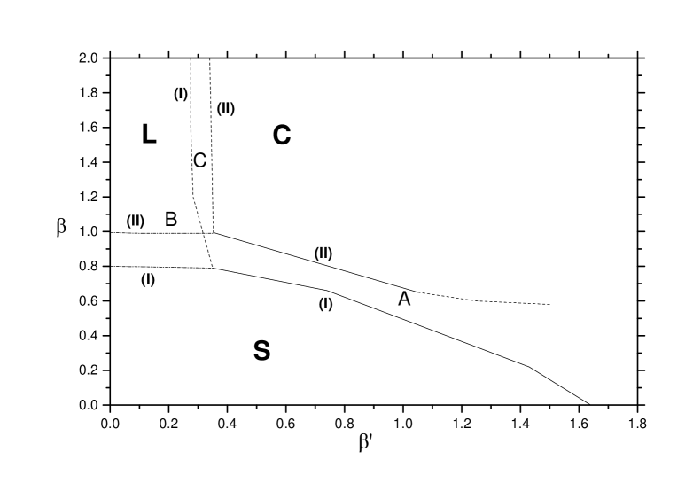
Figure 1: Phase diagram of pure U(1) gauge theory in 4+1 dimensions with anisotropic couplings. Points A, B and C will be studied in detail in the sequel.

We now proceed with a more detailed examination of point A, by performing a hysteresis loop. In figure 2 we show the cycle for the space-like plaquette: $\beta^{\prime}$ is set to 1.0, while $\beta$ runs. The lattice volume used has been $4^{5},$ the step in $\beta$ was 0.01 and 200 sweeps have been made at each point before proceeding to the next one. A big hysteresis loop appears between $\beta=0.56$ and $\beta=0.62,$ indicating a first order transition. Apart from the phase transition it is seen that the space-like plaquette is growing from a value close to zero to a value close to one. Let us just mention that the transverse-like plaquette exhibits a quite similar hysteresis loop between the same values of $\beta$ and its value varies between 0.46 and 0.73.

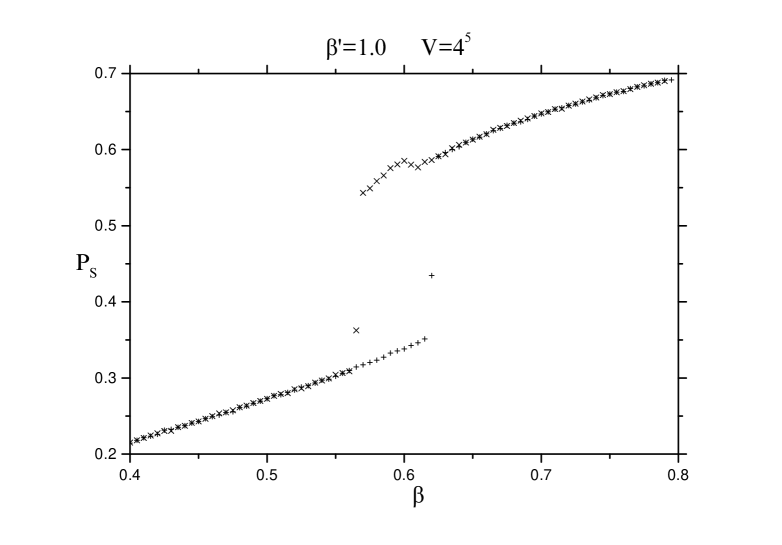
Figure 2: Hysteresis loop for point A of figure 1. The quantity measured is the space-like plaquette.

Of course, more evidence is needed to substantiate our claim that the phase transition from the strong to the Coulomb phase is of first order. This evidence is provided in figure 3, where we show a clear two-state signal in the distribution of the space-like plaquette. This is typical for the values of $\beta$ in the phase transition region.

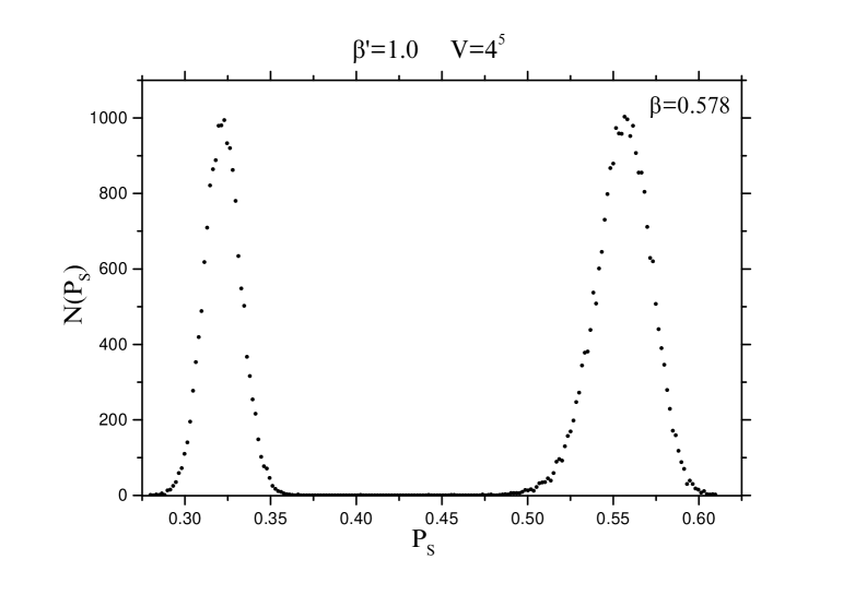
Figure 3: A two-state signal for space-like plaquette for $\beta^{\prime}=1.0$ and $V=4^{5}$ indicating a first order phase transition.

The hysteresis loop relevant for point B of figure 1 is very weak, so we went on to a more detailed study. In figure 4 we show the mean values of the space-like plaquette when $\beta^{\prime}$ is set to 0.2 and $\beta$ takes on several values. The number of thermalization iterations used at each point varied between 10000 and 20000, while the measurements have required 30000 to 50000 sweeps; only the results of one sweep out of five have been taken into account; this means that 6000-10000 measurements have contributed to the mean values. Three volumes have been used: $4^{5},~{}6^{5},~{}8^{5}.$ The curve gets steeper as the volume increases, so a reasonable guess would be that this transition (from the strong to the layered phase) is second order. We mention that the transverse-like plaquette has a small value (about 0.10) in this parameter range. This confirms the picture that gauge fields remain localized along the transverse direction, yielding a large corresponding string tension.

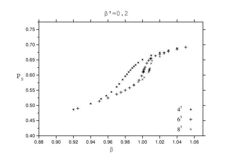
Figure 4: Mean values for the space-like plaquette at point B of figure 1.

Figure 5 contains further elaboration on point B. We have computed the susceptibility of the space-like plaquette for the three lattice volumes $4^{5},~{}6^{5},~{}8^{5}$ to find the volume dependence of the peak of the susceptibility. The number of sweeps needed are the same as the ones in figure 4. It is well known that for a first order phase transition the peak scales with the volume, while for a second order transition the peak scales with a power of the volume smaller than one. The volume ratios read: $\frac{6^{5}}{4^{5}}\simeq 7.59,~{}\frac{8^{5}}{4^{5}}=32.0.$ It is obvious that the ratios of the peaks $(\frac{1.3}{0.6}\simeq 2.16,~{}\frac{1.75}{0.6}\simeq 2.92)$ are much smaller than the corresponding volume ratios, so the transition is of second (or higher) order for the volumes that we have examined. Thus we have here the very interesting possibility of the existence of a continuum limit for this lattice theory along this phase transition line. We comment here that in the $\beta^{\prime}\to 0$ limit we recover the 4-D U(1) pure gauge model. Recent simulations [32] (see also [33]) have shown that the phase transition of the 4-D model is of second order, which matches very well with our result that the strong-layered phase transition is of second order. In particular, the 4-D U(1) phase transition may be considered as a shadow of the strong-layered phase transition. We also note here that the phase transition point ($\beta\simeq 1.0$) is very close to the prediction of the one-loop mean field result (curve (II) of figure 1) and rather far from the zero order mean field (curve (I) of figure 1). This transition has also been characterized as second order in [34] by measuring hysteresis loops for Polyakov line correlators.

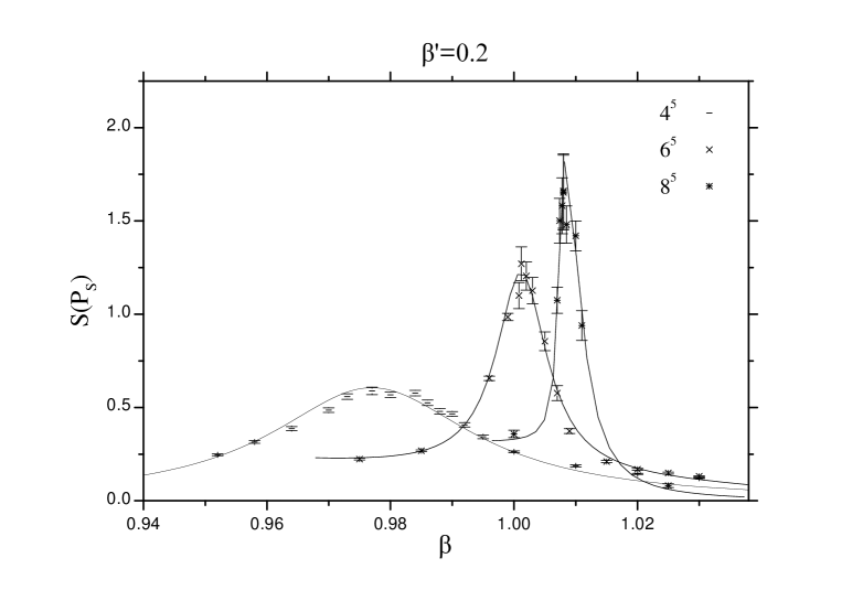
Figure 5: Volume dependence of the susceptibility of the space-like plaquette. The critical point B of figure 1 (strong-layered transition) is relevant here.

In figure 6 we show the Binder cumulant of the space-like plaquette to have an additional check on the strength of the layered-Coulomb transition. For a first order transition the cumulant has a minimum at the critical point, which retains its depth with increasing volume. A second order transition is characterized by the decrease of the depth of the dip. In our figure we observe that the minimum get shallower with increasing volume, in agreement with the estimate based on the previous figure that the phase transition is of second order.

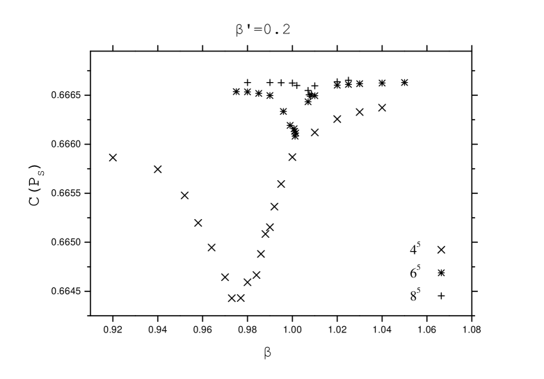
Figure 6: Volume dependence of the Binder cumulant of the space-like plaquette. Also here, as in the previous figure, the critical point B of figure 1 (strong-layered transition) is relevant.

Figure 7 contains mean values in connection with point C of figure 1, which lies on the layered-Coulomb phase transition. The technical details about the number of sweeps are the same as the ones of figure 4 above, but the sensitive quantity is the transverse-like plaquette in this case. Also in this case we used three volumes. The curve grows slightly steeper as the volume increases, but the change is very small. Another feature is that the “critical point” moves to smaller $\beta^{\prime}$ for increasing volume, contrary to the tendency in figure 4. The space-like plaquette is almost constant, varying in the range 0.79-0.80; this is due presumably to the fact that the change happening here is a transition from 4-D to 5-D Coulomb phase, which is not expected to give a great change in the $1\times 1$ plaquette behaviour.

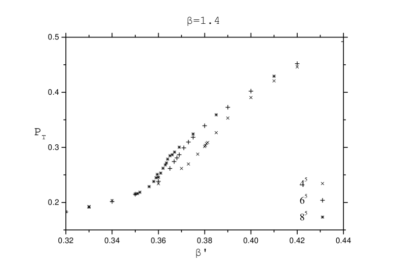
Figure 7: Mean values of the transverse-like plaquette relevant for point C of figure 1 (layered-Coulomb transition).

Since the transition in the previous figure appears very weak, it deserves further more detailed study. In figure 8 we depict the volume dependence of the susceptibility of the transverse-like plaquette. The peaks of the susceptibilities seem to saturate to a final value of about 1.8; in fact this value for the biggest volume is very close to the value 1.4 for the smallest volume, although the volume ratio is 32! It appears that the value of the peak saturates to a definite value, independent of the volume; this could be a signal that the transition is compatible with a crossover.

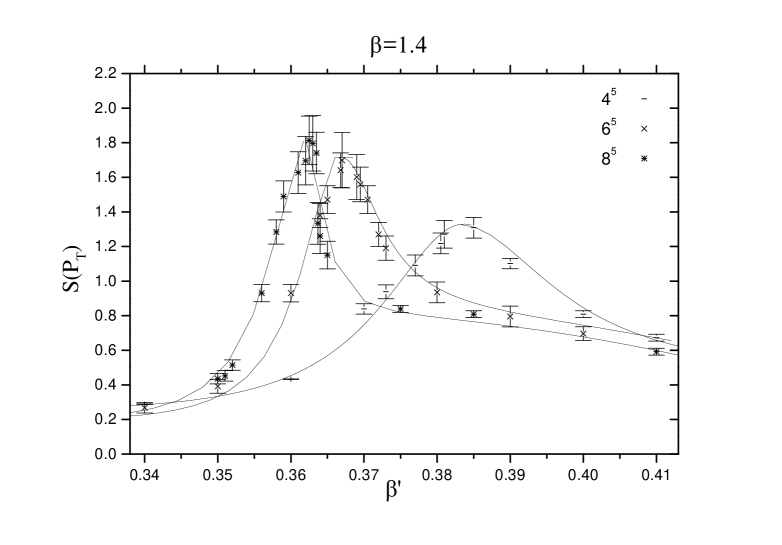
Figure 8: Volume dependence of the susceptibility of the transverse-like plaquette. The critical point C of figure 1 (layered-Coulomb transition) is relevant here.

4.2 Model II

We now pass to model II, which is a model in which $\beta$ and $\beta^{\prime}$ are not independent, as in model I, but are instead related as

$$\beta^{\prime}=\beta e^{-\lambda|n_{T}|}.$$

$\lambda$ is a positive parameter that we change by hand, while $|n_{T}|$ is the (absolute) distance of the current 4-D subspace from a fixed 4-D subspace, used as a reference layer, that is the origin of the ordinate along the transverse direction. Thus the coupling $\beta^{\prime}$ is not constant over the whole extent of the lattice, since it is meant to represent the Randall-Sundrum model.

We have already gained some experience with the behaviour of our model in the case of constant $\beta^{\prime}.$ We have seen there that the new “layered phase” makes its appearance at small values of the $\beta^{\prime}$ parameter. The physical meaning of the layered phase is that the space-like 4-D subspaces (named “layers” for convenience) decouple and behave independently. Now, we expect the same phenomenon to occur when $\beta^{\prime}$ takes small values not only over the whole lattice, but also locally, which is the case of model II. Suppose that we start with the layer which has $n_{T}=0.$ Then $\beta^{\prime}=\beta.$ If we move to layers with $|n_{T}|>0,$ $\beta^{\prime}$ will decrease and it will get its minimum value when we reach the layer with the largest distance from the reference layer. Depending on the value of the $\lambda$ parameter, this value of $\beta^{\prime}$ may be small enough that the layered phase shows up locally. The picture is that the layer with largest $|n_{T}|$ (the most distant layer) will decouple, while its first neighbours (along the transverse direction) will still be connected with the rest of the lattice. If we increase $\lambda,$ we expect that not only the most distant layer, but also the next layer will have small enough $\beta^{\prime}$ for decoupling. If the $\lambda$ parameter grows bigger and bigger we expect that more and more layers will decouple.

We have used the mean values of the space-like and the transverse-like plaquettes, but for model II their definitions are slightly different than the previous ones. The reason is that, because of the dependence of $\beta^{\prime}$ on the transverse coordinate, we should consider these mean values for each layer separately. More precisely, the two operators read:

$${\rm Space-like~{}Plaquette:~{}~{}~{}}{\hat{P}}_{s}(|n_{T}|)\equiv\frac{1}{12N^{4}}\sum_{x,1\leq\mu<\nu\leq 4}\cos F_{\mu\nu}(x)|_{fixed~{}|n_{T}|}$$ (21)

$${\rm Transverse-like~{}Plaquette:~{}~{}~{}}{\hat{P}}_{T}(|n_{T}|)\equiv\frac{1}{8N^{4}}\sum_{x,1\leq\mu\leq 4}\cos F_{\mu T}(x)|_{fixed~{}|n_{T}|}$$ (22)

We have used the mean values $P_{s}(|n_{T}|)\equiv<{\hat{P}}_{s}>|_{fixed~{}|n_{T}|}$ and $P_{t}(x_{t})\equiv<{\hat{P}}_{t}>|_{fixed~{}|n_{T}|}.$

We will study two cases of model II, corresponding to the cases of model I that have already been examined. Figure 9 contains the space-like plaquette ${\hat{P}}_{s}(|n_{T}|)$ versus $\lambda$ if $\beta^{\prime}=0.2$ (point B of figure 1) and the lattice volume is $6^{5}.$ Then $\beta=\beta^{\prime}e^{\lambda|n_{T}|}.$ For this particular lattice size, since the reference layer has $n_{T}=0,$ the two nearest neighbours have $|n_{T}|$ equal to $1$ and the next ones have $n_{T}$ equal to $2.$ We observe in the figure a decoupling transition at $\lambda$ about 0.8 for the first decoupling layer (the one with $|n_{T}|=2;$ upper curve). At this value of $\lambda$ the layers with $|n_{T}|=1$ have rather small values for $\beta,$ so they do not show any sign of decoupling. However, when $\lambda$ grows even larger, we may see the decoupling transition of these “second layers” at $\lambda\simeq 1.65.$

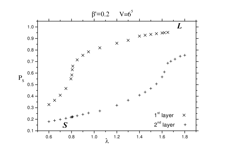
Figure 9: Space-like plaquette versus $\lambda$ for the two values $|n_{T}|=2$ (denoted by “first layer”) and $|n_{T}|=1$ (denoted by “second layer”). $\beta^{\prime}$ is set to 0.2, so we are probing the strong-layered transition. The layered phase lies in the right part of the graph and the strong phase in the left part of it.

A very interesting question is the relation of the layer decoupling phase transitions observed in figure 9 to the corresponding phase transitions of model I. To this end we use the relation between $\beta,~{}\beta^{\prime}$ and $\lambda$ and construct figure 10; this figure is similar to the previous one, the difference being that the horizontal axis is not $\lambda,$ but rather the related variable $\beta.$ In addition, we have put on this graph the results for the mean values of the space-like plaquette for model I (reproduced from figure 3) and the results coming from processing the data of figure 9. The lattice volume $6^{5}$ has been used for all data in figure 10. A striking effect takes place: all three curves lie upon one another. Thus, presumably, the phase transition of model II is nothing more than the corresponding phase transition of model I, if both are expressed in terms of $\beta$ and $\beta^{\prime}.$ In other words, if we revisit the previous figure 9, from the position of $\lambda$ for the first decoupling transition one may determine the values of $\lambda$ for the remaining decoupling transitions, since they correspond to the same value of $\beta.$ It is plausible that the decoupling phase transitions are just the “local” version of the phase transitions which appear in model I: there the parameter $\beta^{\prime}$ has the same value throughout the lattice, so all layers were decoupled from each other simultaneously when $\beta$ took a suitable value. In model II a similar phenomenon takes place locally: the layers do not decouple simultaneously but one after the other.

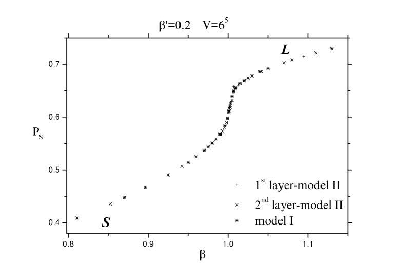
Figure 10: The data of figure 9 plotted versus $\beta.$

Figure 11 is analogous to figure 9, but corresponds to the layered-Coulomb transition (point C of figure 1) rather than the strong-layered one. As a consequence, the relevant quantity is the transverse-like plaquette $P_{T}(|n_{T}|).$ The parameter $\beta$ is set to 1.4 and $\beta^{\prime}$ is found through the relation: $\beta^{\prime}=\beta e^{-\lambda|n_{T}|}.$ This means that $\beta^{\prime}$ at each layer decrease with $\lambda,$ so the corresponding transverse-like plaquette should decrease, which is what we observe. Thus the left part of the graph corresponds roughly to the Coulomb phase, while its right part to the layered phase of figure 1. We observe similar phenomena to figure 9, that is the most distant layer decouples at $\lambda\approx 0.7,$ and the next at $\lambda\approx 1.3.$

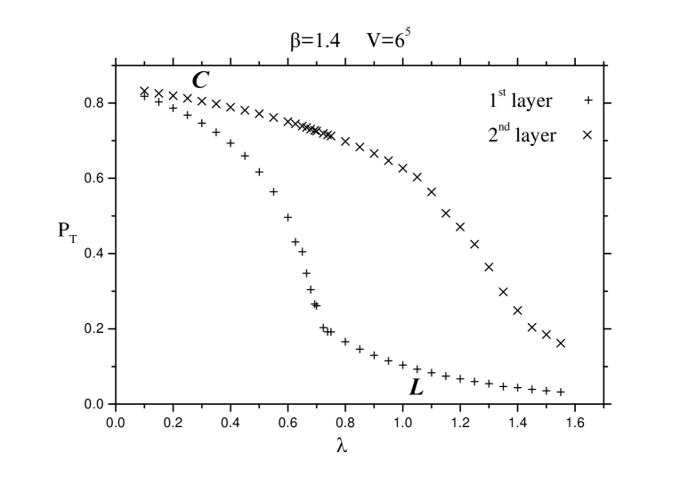
Figure 11: Space-like plaquette versus $\lambda$ for the two values $|n_{T}|=2$ (denoted by “first layer”) and $|n_{T}|=1$ (denoted by “second layer”). $\beta$ is set to 1.4, so we are probing the layered-Coulomb transition. The layered phase lies in the right part of the graph and the Coulomb phase in the left part of it.

Figure 12 is a redrawing of figure 11 in the same way as figure 10 was the redrawing of figure 9. The only difference between figures 11 and 12 is that the mean values are plotted versus $\beta^{\prime}$ rather than versus $\lambda.$ It shows once more that the phase transitions take place at the same values of $\beta^{\prime};$ moreover this value coincides with the critical point of model I. Thus, once more, we find no new phase transitions, but only a “local” version of the old ones; so there is no reason to study this phase transition in more detail, since presumably its characteristics will be the same as the ones of the “global” transition.

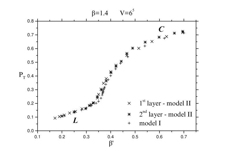
Figure 12: The data of figure 11 plotted versus $\beta.$

5 Conclusions

We have studied here the problem of gauge field localization in the case of anisotropic gauge couplings. We have considered two models, model I and model II. The former has couplings independent from each other and the coordinates, while the latter has an exponentially bigger coupling in the fifth direction. The model I may be realized in a continuum flat homogeneous and anisotropic space, while the model II may be realized in a curved $AdS$ space. Although scalars, fermions as well as gravitons may be localized on a three-brane, at least in the RS background, there is an open question for the gauge bosons. The reason is that a massless gauge field cannot be localized on a brane since it does not depend on the extra dimensions. One of course may imagine a situation in which a Higgs mechanism makes the gauge bosons massive in the bulk and massless inside the brane. However, in this case, a kind of “no-go theorem” does not allow for massless photons on the brane, due to the Meissner effect. In fact, electric fields along the brane dies off exponentially so that there is no Coulomb phase on the brane. A way out is to consider a dual picture where the bulk is in a confining phase (“confining medium” with monopole condensation). In this case the gauge theory on the brane is in a Coulomb phase with massless photons.

In our case, we have considered a five-dimensional pure $U(1)$ gauge theory in the strong phase. We have shown that there is a second order phase transition from the strong phase to a layer phase. The gauge theory along the layer is in the Coulomb phase, while it is still in the strong in the transverse direction. Thus, a four-dimensional massless photon exists on the four-dimensonal layers indicating that localization of the bulk gauge fields has been achieved. This is consistent with the no-go theorem as the gauge theory in the bulk is not in a Higgs phase. Contrary, it is in a strong phase and in a sense may be viewed as realization of the “confining medium” proposal. It should be stressed that one cannot see these effects simply by solving bulk Maxwell equations since the localization of the gauge field is a non-perturbative effect in which strong dynamics is involved. Clearly, such dynamics cannot be captured by any perturbative analysis.

Another mechanism for gauge field localization would be, for example, an $SU(2)$-Higgs model where the theory is in the strong symmetric phase in the bulk and in the Higgs phase on the brane. Moreover, such a picture may also be consistent with a supersymmetric theory in the bulk and broken supersymmetry on the brane.

However, we should keep in mind that although we know that there exists a second order phase transition between the strong and layer phases of the five-dimensional gauge theory, we have not made any detailed study of the continuum limit yet.

Acknowledgements

This work is partially supported by the TMR projects “Finite temperature phase transitions in Particle Physics”, EU contact number: FMRX-CT97-0122, RTN contract RTN-99-0160 and the $\Gamma.\Gamma.E.T$ grand $97E\Lambda/71$. Stimulating discussions with F. Karsch, C.P. Korthals-Altes, S. Nicolis and N. Tetradis are gratefully acknowledged. We also thank V. Stergiou and N. D.Tracas for helpful advice on plotting the numerical data.

References

- [1] I. Antoniadis, Phys. Lett. B 246 (1990)377.
- [2] N. Arkani-Hamed, S. Dimopoulos and G. Dvali, Phys. Lett. B 429 (1998)263, hep-th/9803315; I. Antoniadis, N. Arkani-Hamed, S. Dimopoulos and G. Dvali, Phys. Lett. B 436 (1998)257, hep-th/9804398.
- [3] M. Gell-Mann and B. Zwiebach, Phys. Lett. B141, 333 (1984);Phys. Lett. B147, 111 (1984); Nucl. Phys. B260, 569 (1985).
- [4] H. Nicolai and C. Wetterich, Phys. Lett. B150, 347 (1985).
- [5] A. G. Cohen and D. B. Kaplan, Phys. Lett. B470, 52 (1999), hep-th/9910132.
- [6] A. Kehagias and J. G. Russo, hep-th/0003281.
- [7] E. Witten, hep-ph/0002297.
- [8] L. Randall and R. Sundrum, Phys. Rev. Lett. 83, 4690 (1999), hep-th/9906064; Phys. Rev. Lett. 83, 3370 (1999), hep-ph/9905221.
- [9] M. Lüscher, Nucl. Phys. B180 317 (1981).
- [10] V. Rubakov and M. Shaposhnikov, Phys. Lett. B125 36 (1983).
- [11] C. G. Callan and J. A. Harvey,Nucl. Phys. B250, 427 (1985).
- [12] K. Jansen, Phys. Rept. 273, 1 (1996), hep-lat/9410018.
- [13] A. Barnaveli and O. Kancheli, Sov. J. Nucl. Phys. 51 (1990)573; 52 (1990)576.
- [14] G. Dvali and M. Shifman, Phys. Lett. B396, 64 (1997), hep-th/9612128.
- [15] N. Tetradis, Phys. Lett. B479, 265 (2000), hep-ph/9908209.
- [16] A. Di Giacomo, B. Lucini, L. Montesi, G. Paffuti, Phys.Rev.D61 (2000) 034503; Phys.Rev.D61 (2000) 034504 and references therein.
- [17] W. D. Goldberger and M. B. Wise, Phys. Rev. Lett. 83, 4922 (1999), hep-ph/9907447; Phys. Rev. D60, 107505 (1999), hep-ph/9907218.
- [18] H. Davoudiasl, J. L. Hewett and T. G. Rizzo, Phys. Lett. B473, 43 (2000), hep-ph/9911262.
- [19] T. Gherghetta and A. Pomarol, hep-ph/0003129.
- [20] A. Pomarol, hep-ph/9911294.
- [21] Y.K. Fu and H.B. Nielsen, Nucl. Phys. B 236 167 (1984); Nucl.Phys. B254 (1985) 127.
- [22] C.P.Korthals-Altes, S.Nicolis, J.Prades, Phys.Lett. 316B (1993) 339; A.Huselbos, C.P.Korthals-Altes, S.Nicolis, Nucl.Phys. B450 (1995) 437.
- [23] D. Berman and E. Rabinovici, Phys. Lett. B 157 292 (1985).
- [24] P. Dimopoulos, K. Farakos, C. Korthals-Altes, G. Koutsoumbas and S. Nicolis, “Phase structure of the Abelian Higgs model in 5D with anisotropic couplings”, in preparation.
- [25] J. Maldacena, Adv. Theor. Math. Phys. 2 (1998) 231, hep-th/9711200.
- [26] S.S. Gubser, I.R. Klebanov and A.M. Polyakov, Phys. Lett. B428 (1998)105, hep-th/9802109.
- [27] E. Witten, Adv. Theor. Math. Phys. 2 (1998) 253, hep-th/9802150.
- [28] A. Kehagias, Phys. Lett. B469, 123 (1999), hep-th/9906204; hep-th/9911134.
- [29] G.K. Leontaris and N.E. Mavromatos, Phys. Rev. D61, 124004 (2000), hep-th/9912230.
- [30] M.Creutz, Phys.Rev. D36 (1987) 515.
- [31] F.Brown, T.Woch, Phys.Rev.Lett. 58 (1987) 2394.
- [32] J.Jersak, C.B.Lang, T.Neuhaus, Phys.Rev.Lett. 77 (1996) 1933; Phys.Rev. D54 (1996) 6909; J.Cox, W. Franzki, J.Jersak, C.B.Lang, T.Neuhaus, P.W.Stephenson, Nucl.Phys. B499 (1997) 371.
- [33] J.Ambjorn, D.Espriu and N.Sasakura, Mod.Phys.Lett. A12(1997)2665.
- [34] A.Hulsebos, 1994 Lattice conference, Nucl.Phys. (Proc.Suppl.) 42 (1995) 618.