Noncommutative Korteweg-de-Vries equation

Abstract

We construct a deformation quantized version (ncKdV) of the KdV equation which possesses an infinite set of conserved densities. Solutions of the ncKdV are obtained from solutions of the KdV equation via a kind of Seiberg-Witten map. The ncKdV is related to a modified ncKdV equation by a noncommutative Miura transformation.

1 Introduction

Field theories on noncommutative spaces and more specifically Moyal deformed space-times, gained a lot of interest recently because of the appearance of such theories as certain limits of string, D-brane and M theory (see [1] and the references cited there). In this letter we apply deformation quantization [2] to a classical integrable model, the KdV equation. The passage from commutative to noncommutative space-time is achieved by replacing the ordinary commutative product in the space of smooth functions on $\mathbb{R}^{2}$ with coordinates $t,x$ by the noncommutative associative (Moyal) $\ast$-product [2] which is defined by

$$f\ast h={\bf m}\circ e^{\vartheta P/2}(f\otimes h)$$ (1.1)

where $\vartheta$ is a real or imaginary constant and

$${\bf m}(f\otimes h)=f\,h\,,\qquad P=\partial_{t}\otimes\partial_{x}-\partial_{x}\otimes\partial_{t}\;.$$ (1.2)

An essential ingredient of our deformation of the KdV equation is the concept of a bicomplex. This is an ${\mathbb{N}}_{0}$-graded linear space (over ${\mathbb{R}}$ or ${\mathbb{C}}$) $M=\bigoplus_{r\geq 0}M^{r}$ together with two linear maps ${\rm d},\delta\,:\,M^{r}\rightarrow M^{r+1}$ satisfying

$${\rm d}^{2}=0\,,\qquad\delta^{2}=0\,,\qquad{\rm d}\,\delta+\delta\,{\rm d}=0\;.$$ (1.3)

Associated with a bicomplex is the linear equation

$$\delta\chi=\lambda\,{\rm d}\,\chi$$ (1.4)

where $\chi\in M^{0}$. Let us assume that it admits a (non-trivial) solution as a (formal) power series $\chi=\sum_{m\geq 0}\lambda^{m}\chi^{(m)}$ in $\lambda$. The linear equation then leads to

$$\delta\chi^{(0)}=0\,,\quad\delta\chi^{(m)}={\rm d}\chi^{(m-1)}\,,\quad m=1,\ldots,\infty\;.$$ (1.5)

As a consequence, $J^{(m+1)}={\rm d}\chi^{(m)}$ ($m=0,\ldots,\infty$) are $\delta$-exact. These elements of $M^{1}$ should be regarded as generalized conserved currents (see [3, 4]).

Starting with a certain trivial bicomplex, a dressing (in the sense of [4]) which involves the $\ast$-product results in bicomplex equations which are equivalent to a deformed KdV equation. As a consequence of the underlying bicomplex structure, it shares with the classical equation the property of possessing an infinite set of conservation laws which is a characteristic property of soliton equations. The same procedure has been applied in [6, 7] to obtain “quantized” versions of other integrable models.

In section 2 we derive the ncKdV equation and demonstrate the existence of an infinite set of conservation laws. Section 3 shows how solutions of the KdV equation determine solutions of the ncKdV equation. This is similar to the Seiberg-Witten map between commutative and noncommutative gauge field theories [1]. In particular, we find that the one-soliton KdV solution is also an exact solution of the ncKdV equation. For the KdV two-soliton solution, however, there are corrections involving the deformation parameter. Several familiar classical structures generalize to the noncommutative framework. This concerns in particular the relation between the KdV and the modified KdV equation via the Miura transformation, as shown in section 4. Finally, section 5 contains some conclusions.

2 The KdV equation in noncommutative space-time

We choose the bicomplex space as $M=M^{0}\otimes\Lambda$ where $M^{0}=C^{\infty}({\mathbb{R}^{2}})$ and $\Lambda=\bigoplus_{r=0}^{2}\Lambda^{r}$ is the exterior algebra of a $2$-dimensional vector space with basis $\tau,\xi$ of $\Lambda^{1}$ (so that $\tau^{2}=\xi^{2}=\tau\,\xi+\xi\,\tau=0$). It is then sufficient to define bicomplex maps ${\rm d}$ and $\delta$ on $M^{0}$ since by linearity and ${\rm d}(f\,\tau+h\,\xi)=({\rm d}f)\,\tau+({\rm d}h)\,\xi$ (and correspondingly for $\delta$) for smooth functions $f,h$ they extend to the whole of $M$.

Let us start with the trivial bicomplex which is given by

$${\rm d}f = -f_{xx}\,\xi+(f_{t}+4\,f_{xxx})\,\tau$$ (2.1)

$$\delta f = f_{x}\,\xi-3\,f_{xx}\,\tau$$ (2.2)

where a subscript denotes partial differentiation, e.g., $f_{xx}=\partial_{x}^{2}f$ with $\partial_{x}=\partial/\partial x$. Now we apply a dressing [4] to the bicomplex map ${\rm d}$,

$${\rm D}f = {\rm d}f+\delta(\phi\ast f)-\phi\ast\delta f$$ (2.3)

$$= (-f_{xx}+u\ast f)\,\xi+(f_{t}+4\,f_{xxx}-6\,u\ast f_{x}-3\,u_{x}\ast f)\,\tau$$

where $\phi$ is a function and $u=\phi_{x}$. Here we used that the partial derivatives $\partial_{x}$ and $\partial_{t}$ are derivations with respect to the $\ast$-product. The only nontrivial bicomplex equation is now ${\rm D}^{2}=0$ which is equivalent to the noncommutative KdV (ncKdV) equation

$$u_{t}+u_{xxx}-3\,(u\ast u_{x}+u_{x}\ast u)=0\;.$$ (2.4)

The linear system $\delta\chi=\lambda\,{\rm D}\chi$ associated with the ncKdV equation reads

$$\chi_{x}=\lambda\,(u\ast\chi-\chi_{xx})\,,\qquad\chi_{xx}=-{1\over 3}\,\lambda\,(\chi_{t}+4\,\chi_{xxx}-6\,u\ast\chi_{x}-3\,u_{x}\ast\chi)\;.$$ (2.5)

Now we introduce functions $p$ and $q$ such that

$$\chi_{t}=-\lambda\,p\ast\chi\,,\qquad\chi_{x}=\lambda\,q\ast\chi$$ (2.6)

assuming that $\chi$ is $\ast$-invertible. From $\chi_{tx}=\chi_{xt}$ and (2.6) we find

$$q_{t}+p_{x}-\lambda\,(q\ast p-p\ast q)=0\;.$$ (2.7)

Using the product [8, 7] defined by

$$f\diamond h={\bf m}\circ\frac{\sinh(\vartheta P/2)}{\vartheta P/2}(f\otimes h)$$ (2.8)

this can be written in the form of a conservation law as follows,

$$w_{t}+(p+\lambda\,\vartheta\,q\diamond p_{t})_{x}=0$$ (2.9)

where

$$w=q-\lambda\,\vartheta\,q\diamond p_{x}\;.$$ (2.10)

In terms of $p$ and $q$, the equations (2.5) take the form

$$q = u-\lambda\,q_{x}-\lambda^{2}q\ast q$$ (2.11)

$$p = q_{xx}+3\,q\ast q-6\,u\ast q+\lambda\,(5\,q_{x}\ast q+q\ast q_{x})+4\,\lambda^{2}\,q\ast q\ast q$$ (2.12)

$$= q_{xx}-q\ast q-2\,u\ast q+\lambda\,(q\ast q)_{x}$$

where (2.11) has been used twice to simplify the expression for $p$. Let us expand $p$ and $q$ into power series in $\lambda$,

$$p=\sum_{m=0}^{\infty}\lambda^{m}\,p^{(m)}\,,\qquad q=\sum_{m=0}^{\infty}\lambda^{m}\,q^{(m)}\;.$$ (2.13)

Then (2.11) leads to

$$q^{(0)}=u\,,\qquad q^{(1)}=-u_{x}$$ (2.14)

and

$$q^{(m)}=-q^{(m-1)}_{x}-\sum_{k=0}^{m-2}q^{(k)}\ast q^{(m-2-k)}$$ (2.15)

for $m>1$. From (2.12) we get

$$p^{(0)}=u_{xx}-3\,u\ast u\,,\qquad p^{(1)}=-u_{xxx}+2\,u_{x}\ast u+4\,u\ast u_{x}$$ (2.16)

and

$$p^{(m)}=q^{(m)}_{xx}-2\,u\ast q^{(m)}-\sum_{k=0}^{m}q^{(k)}\ast q^{(m-k)}+\sum_{k=0}^{m-1}\left(q^{(k)}\ast q^{(m-1-k)}\right)_{x}$$ (2.17)

for $m\geq 1$. These formulas allow the recursive calculation of the functions $p^{(m)}$ and $q^{(m)}$ in terms of $u$ and its derivatives. From (2.10) with $w=\sum_{m\geq 0}w^{(m)}$ we now obtain the following expressions for the conserved densities,

$$w^{(0)} = q^{(0)}=u\,,\qquad w^{(1)}=-u_{x}-\vartheta\,u\diamond[u_{xxx}-3\,(u\ast u)_{x}]$$ (2.18)

$$w^{(m)} = q^{(m)}-\vartheta\,\sum_{k=0}^{m-1}q^{(k)}\diamond p^{(m-1-k)}_{x}\qquad(m\geq 1)\;.$$ (2.19)

3 From KdV solutions to ncKdV solutions

In this section we show that every solution of the KdV equation determines a solution of the ncKdV equation.

Let $u^{\prime}=\partial u/\partial\vartheta$. Differentiation of (2.4) with respect to $\vartheta$ leads to

$${u^{\prime}}_{t}+{u^{\prime}}_{xxx}-3\,(u^{\prime}\ast u+u\ast u^{\prime})_{x}-{3\over 2}\,[u_{t},u_{x}]_{x}=0$$ (3.1)

where

$$[f,h]=f\ast h-h\ast f\;.$$ (3.2)

Using the identity

$$3\,[u_{t},u_{x}]=[u,u_{x}]_{t}+[u,u_{x}]_{xxx}-3\,\left([u,u_{x}]_{x}\ast u+u\ast[u,u_{x}]_{x}\right)$$ (3.3)

(3.1) can be rewritten as

$$z_{t}+z_{xxx}-3\,(z\ast u+u\ast z)_{x}=0$$ (3.4)

where

$$z=u^{\prime}-{1\over 2}\,[u,u_{x}]_{x}=u^{\prime}-{1\over 2}\,[u,u_{xx}]\;.$$ (3.5)

(3.4) is linear in $z$ and homogeneous. It admits the solution $z=0$, i.e.,

$$u^{\prime}={1\over 2}\,[u,u_{xx}]\;.$$ (3.6)

Let us define

$$u_{m}=\left.{\partial^{m}u\over\partial\vartheta^{m}}\right|_{\vartheta=0}\qquad(m\geq 0)\;.$$ (3.7)

Lemma. As a consequence of (3.6) we have $u_{2m+1}=0$ for all $m\geq 0$ and, for $m>0$,

$$u_{2m} = \sum_{k=0}^{m-1}{1\over 2^{2k+1}}\,{2m-1\choose 2k+1}\,\sum_{j=0}^{m-k-1}{2(m-k-1)\choose 2j}\sum_{i=0}^{2k+1}{2k+1\choose i}$$ (3.8)

$$(-1)^{2k-i+1}\left(\partial_{t}^{i}\partial_{x}^{2k-i+1}u_{2j}\right)\left(\partial_{t}^{2k-i+1}\partial_{x}^{i+2}u_{2(m-k-j-1)}\right)\;.$$

Proof: Using (3.6) and $u\ast u_{xx}-u_{xx}\ast u=2\,{\bf m}\circ\sinh(\vartheta P/2)\,(u\otimes u_{xx})$, one finds

$${\partial^{2m+1}u\over\partial\vartheta^{2m+1}}={\partial^{2m}\over\partial\vartheta^{2m}}{\bf m}\circ\sinh(\vartheta P/2)\,(u\otimes u_{xx})$$

which implies

$$u_{2m+1}=\sum_{k=0}^{m-1}{2m\choose 2k+1}\,2^{-(2k+1)}\,{\bf m}\circ P^{2k+1}\,\left.{\partial^{2(m-k)-1}\over\partial\vartheta^{2(m-k)-1}}(u\otimes u_{xx})\right|_{\vartheta=0}\;.$$

The summands on the rhs all have a factor consisting of an odd number of derivatives with respect to $\vartheta$ acting on $u\otimes u_{xx}$ according to the product rule of differentiation. This results in a sum of terms each of which has at least one odd derivative of $u$ or $u_{xx}$ as a factor. Using $u^{\prime}|_{\vartheta=0}=0$ which follows from (3.6), our first assertion follows by induction. A similar calculation shows that, for $m>0$,

$$u_{2m}=\sum_{k=0}^{m-1}2^{-(2k+1)}\,{2m-1\choose 2k+1}\sum_{j=0}^{m-k-1}{2(m-k-1)\choose 2j}\,{\bf m}\circ P^{2k+1}\left(u_{2j}\otimes u_{2(m-k-j-1),xx}\right)$$

taking $u_{2m+1}=0$ into account. Using the definition of $P$, we obtain the formula (3.8).  

Now we have the following result: to every solution $u_{0}$ of the classical KdV equation there is a solution of the ncKdV equation at least as a formal power series in $\vartheta$,

$$u=u_{0}+{1\over 2}\,\vartheta^{2}\,u_{2}+{1\over 4!}\,\vartheta^{4}\,u_{4}+\ldots$$ (3.9)

where the functions $u_{2m}$, $m>0$, have to be defined by (3.8). Hence, (3.6) yields a transformation from the commutative KdV to the noncommutative model which is similar to the map considered by Seiberg and Witten in [1] (see section 3.1 there, in particular).

Let us consider the one-soliton solution of the classical KdV equation,

$$u_{0}(x,t)=-2\,k^{2}\,\mbox{sech}^{2}(k\,x-4\,k^{3}\,t)$$ (3.10)

where $k$ is a constant. In this case also the “even” coefficients (3.8) all vanish. For example,

$$u_{2}={1\over 2}\,(u_{0,t}\,u_{0,xxx}-u_{0,x}\,u_{0,xxt})$$ (3.11)

vanishes since $x$ and $t$ enter the one-soliton solution only through a single linear combination. One can also use an argument similar to that in [7], section 5, to verify that (3.10) is indeed an exact solution of the ncKdV equation.

A two-soliton solution of the KdV equation is

$$u_{0}(x,t)=-12\,{3+4\,\cosh(2x-8t)+\cosh(4x-64t)\over[3\,\cosh(x-28t)+\cosh(3x-36t)]^{2}}$$ (3.12)

(see [9], for example). In this case we get

$$u_{2}=331776\,{(\cosh[3\,x-36\,t]-3\,\cosh[x-28\,t])\,(\sinh[3\,x-36\,t]+\sinh[x-28\,t])^{2}\over(\cosh[3\,x-36\,t]+3\,\cosh[x-28\,t])^{5}}$$ (3.13)

with the help of Mathematica. In particular, the second order ncKdV correction to the above two-soliton KdV solution does not vanish. Plots of the two-soliton KdV solution and its ncKdV correction $u_{2}$, produced with Mathematica, are shown in Fig. 1 and Fig. 2, respectively.

For the forth order ncKdV correction to the two-soliton KdV solution we get

$$u_{4} = {3\over 2}\,(u_{2,t}\,u_{0,xxx}-u_{2,x}\,u_{0,txx}+u_{0,t}\,u_{2,xxx}-u_{0,x}\,u_{2,txx})$$ (3.14)

$$+{1\over 8}\,(u_{0,ttt}\,u_{0,xxxxx}-3\,u_{0,ttx}\,u_{0,txxxx}+3\,u_{0,txx}\,u_{0,ttxxx}-u_{0,xxx}\,u_{0,tttxx})$$

which results in a lengthy expression in terms of hyperbolic functions. This function is plotted in Fig. 3. There is a strong similarity between $u_{2}$ and $u_{4}$. The plots show that $u_{2}$ and $u_{4}$ vanish as $t\to\pm\infty$. Indeed, since an $N$-soliton solution $u_{0}$ of the KdV equation asymptotically (as $t\to\pm\infty$) separates into single solitons, the ncKdV corrections $u_{2m}$, $m>0$, tend to zero by (3.8) and the properties of a single soliton solution.

4 Noncommutative Miura transformation and noncommutative modified KdV equation

An obvious analogue of the classical Miura transformation in the noncommutative framework is

$$u=v_{x}+v\ast v\;.$$ (4.1)

With its help one finds

$$\mbox{ncKdV}(u)=(\mbox{ncmKdV}(v))_{x}+v\ast(\mbox{ncmKdV}(v))+(\mbox{ncmKdV}(v))\ast v$$ (4.2)

where $\mbox{ncKdV}(u)$ stands for the left hand side of (2.4) and

$$\mbox{ncmKdV}(v)=v_{t}+v_{xxx}-3\,(v\ast v\ast v_{x}+v_{x}\ast v\ast v)\;.$$ (4.3)

Hence, if $v$ solves the noncommutative modified KdV (ncmKdV) equation

$$\mbox{ncmKdV}(v)=0$$ (4.4)

then $u$ solves the ncKdV equation. Differentiation of the Miura transformation with respect to $\vartheta$ leads to

$$u^{\prime}=v^{\prime}_{x}+v^{\prime}\ast v+v\ast v^{\prime}+{1\over 2}\,[v_{t},v_{x}]$$ (4.5)

so that (3.5) translates to

$$v^{\prime}={1\over 2}\,\left([v\ast v,v_{xx}]-[v,v_{x}\ast v_{x}]\right)+r$$ (4.6)

where

$$z=r_{x}+r\ast v+v\ast r\;.$$ (4.7)

Differentiating (4.4) with respect to $\vartheta$, a lengthy calculation shows that the resulting equation is satisfied as a consequence of (4.6) with $r=0$. This means that we have a construction of ncmKdV solutions from mKdV solutions in complete analogy to the ncKdV case treated in the previous section.

Instead of the noncommutative Miura transformation we can consider the analogue of the Gardner transformation (cf [9])

$$u=q+\lambda\,q_{x}+\lambda^{2}\,q\ast q$$ (4.8)

which is precisely our equation (2.11). Then one finds

$$\mbox{ncKdV}(u)=\left(1+\lambda\,\partial_{x}+\lambda^{2}\,\{q,\cdot\}\right)\,\mbox{ncKdV}(q;\lambda)$$ (4.9)

where $\{f,h\}=f\ast h+h\ast f$ and

$$\mbox{ncKdV}(q;\lambda)=q_{t}+q_{xxx}-3\,(q\ast q)_{x}-3\,\lambda^{2}\,(q\ast q\ast q_{x}+q_{x}\ast q\ast q)\;.$$ (4.10)

As a consequence, $u$ satisfies the ncKdV equation if $q$ is a solution of the noncommutative generalized KdV equation

$$\mbox{ncKdV}(q;\lambda)=0\;.$$ (4.11)

Using the identity

$$3\,(q\ast q\ast q_{x}+q_{x}\ast q\ast q)=2\,(q\ast q\ast q)_{x}+[q,[q,q_{x}]]$$ (4.12)

and (2.8), the latter equation can be rewritten in the form of a conservation law as follows,

$$\tilde{w}_{t}+(q_{xx}-3\,q\ast q-2\,\lambda^{2}\,q\ast q\ast q+\lambda^{2}\vartheta\,q_{t}\diamond[q,q_{x}])_{x}=0$$ (4.13)

where

$$\tilde{w}=q-\lambda^{2}\vartheta\,q_{x}\diamond[q,q_{x}]\;.$$ (4.14)

This expression is different from the conserved density $w$ given in (2.10). However, $\tilde{w}$ and $w$ must be equal up to a total $x$-derivative.

5 Conclusions

We obtained a (Moyal) deformed version of the KdV equation which lives on a noncommutative space-time and which shares with its classical version the property of having an infinite set of conserved densities, a characteristic feature of soliton equations and (infinite-dimensional) integrable models. Indeed, the soliton structure of the KdV equation is essentially preserved under the deformation so that the ncKdV equation is a very concrete example of a “noncommutative soliton equation”. More precisely, given a solution of the KdV equation, there is a prescription how to calculate from it a corresponding solution of the ncKdV equation order by order in $\vartheta$. In particular, the one-soliton solution of the KdV equation is also an exact solution of the ncKdV equation (without $\vartheta$-corrections). For the two-soliton solution, corrections of even order in the deformation parameter $\vartheta$ arise from the ncKdV equation which lead to modifications in the strong interaction region of the solitons. In principle, such modulations could be observed in a physical system. Furthermore, it is quite surprising that the relation between the KdV and the mKdV equation via the Miura transformation, as well as the construction of conserved densities via the Gardner transformation passes over to the noncommutative equations.

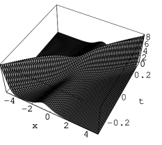
Figure 1: Plot of the two-soliton KdV solution. More precisely, the plot shows $-u_{0}$.

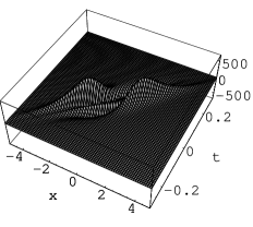
Figure 2: Plot of the second order ncKdV correction $u_{2}$ to the two-soliton KdV solution.

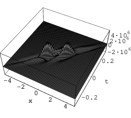
Figure 3: Plot of the forth order ncKdV correction $u_{4}$ to the two-soliton KdV solution.

References

• [1] N. Seiberg and E. Witten, String theory and noncommutative geometry, JHEP 09 (1999) 032.
• [2] F. Bayen, M. Flato, C. Fronsdal, A. Lichnerowicz and D. Sternheimer, Deformation theory and quantization I, II, Ann. Phys. 111 (1978) 61–151.
• [3] A. Dimakis and F. Müller-Hoissen, Bi-differential calculi and integrable models, J. Phys. A: Math. Gen. 33 (2000) 957–974.
• [4] A. Dimakis and F. Müller-Hoissen, Bicomplexes and integrable models, nlin.SI/0006029.
• [5] A. Dimakis and F. Müller-Hoissen, Bi-differential calculus and the KdV equation, math-ph/9908016, to appear in Rep. Math. Phys..
• [6] A. Dimakis and F. Müller-Hoissen, Bicomplexes, integrable models, and noncommutative geometry, hep-th/0006005.
• [7] A. Dimakis and F. Müller-Hoissen, A noncommutative version of the nonlinear Schrödinger equation, hep-th/0007015.
• [8] I.A.B. Strachan, A geometry of multidimensional integrable systems, J. Geom. Phys. 21 (1997) 255–278.
• [9] P.G. Drazin and R.S. Johnson, Solitons: an Introduction, Cambridge University Press, Cambridge, 1989.
• [10] S. Wolfram, The Mathematica Book, 4th ed., Cambridge University Press, Cambridge, 1999.
Refer to caption