A Note on the Weyl Anomaly
in the Holographic Renormalization Group

Masafumi Fukuma, So Matsuura and Tadakatsu Sakai

Yukawa Institute for Theoretical Physics,
Kyoto University, Kyoto 606-8502, Japan

ABSTRACT

We give a prescription for calculating the holographic Weyl anomaly in arbitrary dimension within the framework based on the Hamilton-Jacobi equation proposed by de Boer, Verlinde and Verlinde. A few sample calculations are made and shown to reproduce the results that are obtained to this time with a different method. We further discuss continuum limits, and argue that the holographic renormalization group may describe the renormalized trajectory in the parameter space. We also clarify the relationship of the present formalism to the analysis carried out by Henningson and Skenderis.

1 Introduction

The AdS/CFT correspondence [1] (for a review see Ref. [2]) states that a gravitational theory on the $(d+1)$-dimensional anti-de-Sitter space (AdS_d+1) has a dual description in terms of a conformal field theory on the $d$-dimensional boundary. One of the most significant aspects of the AdS/CFT correspondence is that it can further give us a framework to study the renormalization group (RG) structure of the boundary field theories [3][4][5][6][7][8][9][10][11]. In this scheme of the “holographic RG,” the extra radial coordinate in the bulk is regarded as parametrizing the RG flow of the dual boundary field theory, and the evolution of bulk fields along the radial direction is considered as describing the RG flow of the coupling constants in the boundary field theory.

In Ref. [12], de Boer, Verlinde and Verlinde proposed the formulation of the holographic RG based on the Hamilton-Jacobi equation. They showed, by investigating five-dimensional gravity with scalar fields, that the Callan-Symanzik equation of the four-dimensional boundary theory actually arises from the holographic RG. They also calculated the Weyl anomaly in four dimensions and found that the result agrees with those given in Ref. [13] (see Ref. [14] for a review of the Weyl anomaly). The extension of their analysis to a system including gauge fields is discussed in Ref. [15].

The first main aim of the present note is to give a prescription for calculating the Weyl anomaly in arbitrary dimension, within the framework based on the Hamilton-Jacobi equation. This prescription is actually a simple generalization of the algorithm given in Ref. [12] for the four-dimensional case. Here we carry out a few sample calculations to affirm its correctness.

Second, we give discussion on continuum limits, and show that when bare couplings are tuned such that they are on the classical trajectories passing through the corresponding renormalized couplings, both the bare and renormalized couplings satisfy an RG equation of the same functional form. This fact strongly suggests that the holographic RG may directly describe the so-called renormalized trajectory [16] in the parameter space.

Finally, we discuss the relationship among various renormalizations adopted in the literature on the holographic RG. In particular, we give a detailed analysis of the relationship between the analysis based on the Hamilton-Jacobi equation and that carried out by Henningson and Skenderis [13].

The organization of this note is as follows. In §2, we give a review of the flow equation that is obtained from the Hamilton-Jacobi equation [12]. In §3, we describe a prescription for solving the flow equation and make sample calculations of the Weyl anomaly in four and six dimensions. The results are found to agree with those given in Ref. [13]. In §4, we explore the continuum limits of the boundary field theory in the context of the holographic RG. In §5, we investigate the relationship among various renormalizations. In particular, we give a detailed discussion of the relation between the present analysis and that given in Ref. [13]. Section 6 is devoted to conclusions. The appendices are meant to make this note as self-contained as possible.

2 Hamilton-Jacobi constraint and the flow equation

In this section, we briefly review the formulation of the holographic RG based on the Hamilton-Jacobi equation [12], with the purpose of fixing our convention.

We start by recalling the Euclidean ADM decomposition that parametrizes a $(d+1)$-dimensional metric as

$$ds^{2} = \mbox{\boldmath$G$}_{M\!N}\,dX^{M}dX^{N}$$ (2.1)

$$= N(x,r)^{2}dr^{2}+G_{\mu\nu}(x,r)\Bigl{(}dx^{\mu}+\lambda^{\mu}(x,r)dr\Bigr{)}\Bigl{(}dx^{\nu}+\lambda^{\nu}(x,r)dr\Bigr{)}.$$

Here $X^{M}=(x^{\mu},r)$ with $\mu,\nu=1,2,\cdots,d$, and $N$ and $\lambda^{\mu}$ are the lapse and the shift function, respectively. The signature of the metric $G_{\mu\nu}$ is taken to be $(+\cdots+)$. As we discussed in the Introduction, the Euclidean time $r$ is identified with the RG parameter of the $d$-dimensional boundary theory, and the evolution of bulk fields in $r$ is identified with the RG flow of the coupling constants of the boundary theory. In the following discussion, we exclusively consider scalar fields as such bulk fields.

The Einstein-Hilbert action with bulk scalars $\phi^{i}(x,r)$ on a $(d+1)$-dimensional manifold $M_{d+1}$ with boundary $\Sigma_{d}=\partial M_{d+1}$ is given by

$$S_{d+1}[\mbox{\boldmath$G$}_{M\!N}(x,r),\phi^{i}(x,r)]$$

$$~{}~{}~{}~{}~{}=\int_{M_{d+1}}d^{d+1}X\sqrt{\mbox{\boldmath$G$}}\left(V(\phi)-\mbox{\boldmath$R$}+{1\over 2}\,L_{ij}(\phi)\,\mbox{\boldmath$G$}^{M\!N}\,\partial_{M}\phi^{i}\,\partial_{N}\phi^{j}\right)-2\int_{\Sigma_{d}}d^{d}x\,\sqrt{G}\,K\,,$$

(2.2)

which is expressed in the ADM parametrization as

$$S_{d+1}[G_{\mu\nu}(x,r),\phi^{i}(x,r),N(x,r),\lambda^{\mu}(x,r)]$$

$$~{}~{}~{}=\int d^{d}x\,dr\,\sqrt{G}\,\Bigl{[}\,N\left(V(\phi)-R+K_{\mu\nu}K^{\mu\nu}-K^{2}\right)$$

$$~{}~{}~{}~{}~{}+\,{1\over 2N}\,L_{ij}(\phi)\left(\left(\dot{\phi}^{i}-\lambda^{\mu}\partial_{\mu}\phi^{i}\right)\left(\dot{\phi}^{j}-\lambda^{\mu}\partial_{\mu}\phi^{j}\right)+N^{2}G^{\mu\nu}\partial_{\mu}\phi^{i}\partial_{\nu}\phi^{j}\right)\,\Bigr{]}$$

$$~{}~{}~{}\equiv\int d^{d}x\,dr\,\sqrt{G}\,{\cal L}_{d+1}[G,\phi,N,\lambda],$$ (2.3)

where $\cdot=\partial/\partial r$. Here $R$ and $\nabla_{\mu}$ are the scalar curvature and the covariant derivative with respect to $G_{\mu\nu}$, respectively, and $K_{\mu\nu}$ is the extrinsic curvature on $\Sigma_{d}$ given by

$$K_{\mu\nu}={1\over 2N}\left(\dot{G}_{\mu\nu}-\nabla_{\mu}\lambda_{\nu}-\nabla_{\nu}\lambda_{\mu}\right),\qquad K=G^{\mu\nu}\,K_{\mu\nu}.$$ (2.4)

The boundary term in Eq. (2.2) needs to be introduced to ensure that the Dirichlet boundary conditions can be imposed on the system consistently [17]. In fact, the second derivative in $r$ appearing in the first term of Eq. (2.2) can be written as a total derivative and canceled with the boundary term.

As far as classical solutions are concerned, the action (2.3) is equivalent to the following one in first-order form:

$$S_{d+1}[G_{\mu\nu},\phi^{i},\Pi^{\mu\nu},\Pi_{i},N,\lambda^{\mu}]\equiv\int d^{d}x\,dr\,\sqrt{G}\left[\,\Pi^{\mu\nu}\dot{G}_{\mu\nu}+\Pi_{i}\dot{\phi}^{i}+N{\cal H}+\lambda_{\mu}{\cal P}^{\mu}\,\right],$$

(2.5)

with

$${\cal H} \equiv {1\over d-1}\left(\Pi_{\mu}^{\mu}\right)^{2}-\Pi_{\mu\nu}^{2}-{1\over 2}\,L^{ij}(\phi)\,\Pi_{i}\,\Pi_{j}+V(\phi)-R+{1\over 2}\,L_{ij}(\phi)\,G^{\mu\nu}\,\partial_{\mu}\phi^{i}\,\partial_{\nu}\phi^{j},$$

$${\cal P}^{\mu} \equiv 2\,\nabla_{\nu}\Pi^{\mu\nu}-\Pi_{i}\,\nabla^{\mu}\phi^{i}.$$ (2.6)

In fact, the equations of motion for $\Pi^{\mu\nu}$ and $\Pi_{i}$ give the relations

$$\Pi^{\mu\nu}=K^{\mu\nu}-G^{\mu\nu}K,\qquad\Pi_{i}={1\over N}L_{ij}(\phi)\left(\dot{\phi}^{j}-\lambda^{\mu}\,\partial_{\mu}\phi^{j}\right),$$ (2.7)

and by substituting this expression into Eq. (2.5), we can obtain (2.3). Here $N$ and $\lambda^{\mu}$ simply behave as Lagrange multipliers, giving the Hamiltonian and momentum constraints:

$${1\over\sqrt{G}}\,{\delta S_{d+1}\over\delta N} = {\cal H}~{}=~{}0,$$ (2.8)

$${1\over\sqrt{G}}\,{\delta S_{d+1}\over\delta\lambda_{\mu}} = {\cal P}^{\mu}~{}=~{}0.$$ (2.9)

Note that these constraints generate reparametrizations of the form $r\rightarrow r+\delta r(x),\,x^{\mu}\rightarrow x^{\mu}+\delta x^{\mu}(x)$ for systems on an “equal time slice” $\Sigma_{d}$ ($r={\rm const}$). One can easily show that they are of the first class under the canonical Poisson brackets for $G_{\mu\nu},\Pi^{\mu\nu},\phi^{i}$ and $\Pi_{i}$. Thus, up to gauge equivalent configurations generated by ${\cal H}$ and ${\cal P}^{\mu}$, the $r$-evolution of the bulk fields is uniquely determined, being independent of the values of the Lagrange multiplier $N$ and $\lambda^{\mu}$. In the following discussion, we work in the “temporal gauge,” $N=1,~{}\lambda^{\mu}=0$.

Let $\overline{G}_{\mu\nu}(x,r;G(x),r_{0})$ and $\bar{\phi}^{i}(x,r;\phi(x),r_{0})$ be the classical solutions of the bulk action with the boundary conditions

$$\overline{G}_{\mu\nu}(x,r\!=\!r_{0})=G_{\mu\nu}(x),\qquad\bar{\phi}^{i}(x,r\!=\!r_{0})=\phi^{i}(x).$$ (2.10)

We also define $\overline{\Pi}^{\mu\nu}(x,r)$ and $\overline{\Pi}_{i}(x,r)$ to be the classical solutions of $\Pi^{\mu\nu}(x,r)$ and $\Pi_{i}(x,r)$, respectively. We then define the on-shell action that is obtained as a functional of the boundary values, $G_{\mu\nu}(x)$ and $\phi^{i}(x)$, by substituting these classical solutions into the bulk action:

$$S[G_{\mu\nu}(x),\phi(x),r_{0}]$$

$$~{}\equiv S_{d+1}\left[\overline{G}_{\mu\nu}(x,r;G(x),r_{0}),\,\bar{\phi}^{i}(x,r;\phi(x),r_{0}),\,\overline{\Pi}^{\mu\nu}(x,r),\,\overline{\Pi}_{i}(x,r),\,N(x,r),\,\lambda^{\mu}(x,r)\right]$$

$$~{}=\int d^{d}x\int_{r_{0}}dr\,\sqrt{\overline{G}}\,\,\left[\,\overline{\Pi}^{\mu\nu}\,\dot{\overline{G}}_{\mu\nu}\,+\,\overline{\Pi}_{i}\,\dot{\bar{\phi}}{}^{i}\,\right].$$ (2.11)

Here we have used the Hamiltonian and momentum constraints, $\overline{{\cal H}}=\overline{{\cal P}}_{\mu}=0$. One can see that the variation of the action (2.3) is given by

$$\delta S[G(x),\phi(x),r_{0}] = -\,\int d^{d}x\,\sqrt{\overline{G}}\,\Biggl{[}\,\left(\overline{\Pi}^{\mu\nu}(x,r_{0})\,\dot{\overline{G}}_{\mu\nu}(x,r_{0})+\overline{\Pi}_{i}(x,r_{0})\,\dot{\bar{\phi}}{}^{i}(x,r_{0})\right)\delta r_{0}$$ (2.12)

$$~{}~{}+\,\overline{\Pi}^{\mu\nu}(x,r_{0})\,\delta\overline{G}_{\mu\nu}(x,r_{0})\,+\,\overline{\Pi}_{i}(x,r_{0})\,\delta\bar{\phi}^{i}(x,r_{0})\,\Biggr{]}$$

$$= -\,\int d^{d}x\sqrt{G}\left[\,\overline{\Pi}^{\mu\nu}(x,r_{0})\,\delta G_{\mu\nu}(x)+\overline{\Pi}_{i}(x,r_{0})\,\delta\phi^{i}(x)\,\right],$$

since $\delta\overline{G}_{\mu\nu}(x,r_{0})=\delta G_{\mu\nu}(x)-\dot{\overline{G}}_{\mu\nu}(x,r_{0})\,\delta r_{0}$, etc. It thus follows that the classical conjugate momenta evaluated at $r=r_{0}$ are given by

$$\Pi^{\mu\nu}(x)\equiv\overline{\Pi}^{\mu\nu}(x,r_{0})={-1\over\sqrt{G}}\,{\delta S\over\delta G_{\mu\nu}(x)},\qquad\Pi_{i}(x)\equiv\overline{\Pi}_{i}(x,r_{0})={-1\over\sqrt{G}}\,{\delta S\over\delta\phi^{i}(x)}.$$ (2.13)

We also see that

$${\partial\over\partial r_{0}}S[G_{\mu\nu}(x),\phi^{i}(x),r_{0}]=0.$$ (2.14)

Therefore, the on-shell action $S$ is independent of the coordinate value of the boundary, $r_{0}$. Substituting (2.13) into the Hamiltonian constraint (2.8), we thus obtain the flow equation of de Boer, Verlinde and Verlinde [12],

$$\{S,S\}(x)=\sqrt{G(x)}\,{\cal L}_{d}(x),$$ (2.15)

with

$$\{S,S\}(x) \equiv {1\over\sqrt{G}}\left[\,-\,{1\over d-1}\left(G_{\mu\nu}{\delta S\over\delta G_{\mu\nu}}\right)^{2}+\left({\delta S\over\delta G_{\mu\nu}}\right)^{2}+{1\over 2}L^{ij}(\phi)\,{\delta S\over\delta\phi^{i}}\,{\delta S\over\delta\phi^{j}}\,\right],$$

$${\cal L}_{d}(x) \equiv V(\phi)-R+{1\over 2}\,L_{ij}(\phi)\,G^{\mu\nu}\partial_{\mu}\phi^{i}\partial_{\nu}\phi^{j}.$$ (2.17)

The momentum constraint (2.9) ensures the invariance of $S$ under a $d$-dimensional diffeomorphism along the fixed time slice $r=r_{0}$:

$$\int d^{d}x\,\sqrt{G}\,\left[\left(\nabla_{\mu}\epsilon_{\nu}+\nabla_{\nu}\epsilon_{\mu}\right)\frac{\delta S}{\delta G_{\mu\nu}}+\epsilon^{\mu}\,\partial_{\mu}\phi^{i}\,\frac{\delta S}{\delta\phi^{i}}\right]=0,$$ (2.18)

with $\epsilon^{\mu}(x)$ an arbitrary function.

3 Solution to the flow equation and the Weyl anomaly

In this section, we discuss a systematic prescription for solving the flow equation (2.15).

First we assume that the on-shell action takes the form

$$S[G(x),\phi(x)]=S_{\rm loc}[G(x),\phi(x)]+\Gamma[G(x),\phi(x)],$$ (3.1)

where ${S_{\rm loc}}[G,\phi]$ is part of $S[G,\phi]$ and can be expressed as a sum of local terms:

$$S_{\rm loc}[G(x),\phi(x)] = \int d^{d}x\,\sqrt{G(x)}\,{{\cal L}_{\rm loc}}(x)$$ (3.2)

$$= \int d^{d}x\,\sqrt{G(x)}\sum_{w=0,2,4,\cdots}\bigl{[}{{\cal L}_{\rm loc}}(x)\bigr{]}_{w}.$$

Here we have arranged the sum over local terms according to the weight $w$ that is defined additively from the following rule:

	weight
$G_{\mu\nu}(x),\,\phi^{i}(x),\,\Gamma[G,\phi]$	$0$
$\partial_{\mu}$	$1$
$R,\,R_{\mu\nu},\,\partial_{\mu}\phi^{i}\partial_{\nu}\phi^{j},\,\cdots$	$2$
$\delta\Gamma/\delta G_{\mu\nu}(x),\,\delta\Gamma/\delta\phi^{i}(x)$	$d$

The last line is a natural consequence of the relation $w\!\left(\Gamma[G,\phi]\right)=0$, since $\delta\Gamma=\int d^{d}x\linebreak\left(\delta\phi(x)\times\delta\Gamma/\delta\phi(x)+\cdots\right)$. Then, substituting the above equation into the flow equation (2.15) and comparing terms of the same weight, we obtain a sequence of equations that relate the off-shell bulk action (2.3) to the on-shell boundary action (3.1). They take the following form:

$$\sqrt{G}\,{\cal L}_{d} = \Bigl{[}\left\{{S_{\rm loc}},\,{S_{\rm loc}}\right\}\Bigr{]}_{0}+\Bigl{[}\left\{{S_{\rm loc}},\,{S_{\rm loc}}\right\}\Bigr{]}_{2}\,,$$ (3.3)

$$0 = \Bigl{[}\left\{{S_{\rm loc}},\,{S_{\rm loc}}\right\}\Bigr{]}_{w}\quad(w=4,6,\cdots,d-2),$$ (3.4)

$$0 = 2\Bigl{[}\left\{{S_{\rm loc}},\,\Gamma\right\}\Bigr{]}_{d}+\Bigl{[}\left\{{S_{\rm loc}},\,{S_{\rm loc}}\right\}\Bigr{]}_{d}\,,$$ (3.5)

$$0 = 2\Bigl{[}\left\{{S_{\rm loc}},\,\Gamma\right\}\Bigr{]}_{w}+\Bigl{[}\left\{{S_{\rm loc}},\,{S_{\rm loc}}\right\}\Bigr{]}_{w}\quad(w=d+2,\cdots,2d-2),$$ (3.6)

$$0 = \Bigl{[}\left\{\Gamma,\,\Gamma\right\}\Bigr{]}_{2d}+2\Bigl{[}\left\{{S_{\rm loc}},\,\Gamma\right\}\Bigr{]}_{2d}+\Bigl{[}\left\{{S_{\rm loc}},\,{S_{\rm loc}}\right\}\Bigr{]}_{2d}\,,$$ (3.7)

$$0 = 2\Bigl{[}\left\{{S_{\rm loc}},\,\Gamma\right\}\Bigr{]}_{w}+\Bigl{[}\left\{{S_{\rm loc}},\,{S_{\rm loc}}\right\}\Bigr{]}_{w}\quad(w=2d+2,\cdots).\,$$ (3.8)

Equations  (3.3) and (3.4) determine $\left[{{\cal L}_{\rm loc}}\right]_{w}~{}(w=0,2,\cdots,d-2)$, which together with Eq. (3.5) in turn determine the non-local functional $\Gamma$. Although $\left[{{\cal L}_{\rm loc}}\right]_{d}$ could enter the expression, this would not give a physically relevant effect, as we see below.

By parametrizing $[{{\cal L}_{\rm loc}}]_{0}$ and $[{{\cal L}_{\rm loc}}]_{2}$ as

$$\left[{{\cal L}_{\rm loc}}\right]_{0} = W(\phi),$$ (3.9)

$$\left[{{\cal L}_{\rm loc}}\right]_{2} = -\Phi(\phi)\,R+{1\over 2}\,M_{ij}(\phi)\,G^{\mu\nu}\,\partial_{\mu}\phi^{i}\,\partial_{\nu}\phi^{j},$$ (3.10)

one can easily solve (3.3) to obtain

$$V(\phi) = -{d\over 4(d-1)}\,W(\phi)^{2}+{1\over 2}L^{ij}(\phi)\,\partial_{i}W(\phi)\,\partial_{j}W(\phi)\,,$$ (3.11)

$$-1 = {d-2\over 2(d-1)}\,W(\phi)\,\Phi(\phi)-L^{ij}(\phi)\,\partial_{i}W(\phi)\,\partial_{j}\Phi(\phi)\,,$$ (3.12)

$${1\over 2}\,L_{ij}(\phi) = -{d-2\over 4(d-1)}\,W(\phi)\,M_{ij}(\phi)-L^{kl}(\phi)\,\partial_{k}W(\phi)\,\Gamma^{(M)}_{l;ij}(\phi)\,,$$ (3.13)

$$0 = W(\phi)\,\nabla^{2}\,\Phi(\phi)+L^{ij}(\phi)\,\partial_{i}W(\phi)\,M_{jk}(\phi)\,\nabla^{2}\phi^{k}\,.$$ (3.14)

Here $\partial_{i}=\partial/\partial\phi^{i}$, and $\Gamma^{(M)k}_{ij}(\phi)\equiv M^{kl}(\phi)\,\Gamma^{(M)}_{l;ij}(\phi)$ is the Christoffel symbol constructed from $M_{ij}(\phi)$. For pure gravity ($L_{ij}=0,M_{ij}=0$), for example, setting $V=2\Lambda=-d(d-1)/l^{2}$, we find

$$W=-\,\frac{2\,(d-1)}{l},\quad\Phi=\frac{l}{d-2}.$$ (3.15)

Here $\Lambda$ is the bulk cosmological constant, and when the metric is asymptotically AdS, the parameter $l$ is identified with the radius of the asymptotic AdS_d+1.

To solve Eq. (3.4), we need to introduce local terms of higher weight ($w\geq 4$). For example, for the pure gravity case, we need a local term $[{{\cal L}_{\rm loc}}]_{4}$ of the form

$$[{{\cal L}_{\rm loc}}]_{4}=XR^{2}+YR_{\mu\nu}R^{\mu\nu}+ZR_{\mu\nu\lambda\sigma}R^{\mu\nu\lambda\sigma},$$ (3.16)

with $X,Y$ and $Z$ being some constants to be determined. By using this, we find that

$$\frac{1}{\sqrt{G}}\Bigl{[}\left\{S_{\rm loc},S_{\rm loc}\right\}\Bigr{]}_{4}$$

$$~{}=-{W\over 2(d-1)}\left((d-4)X-{d\,l^{3}\over 4(d-1)(d-2)^{2}}\right)R^{2}$$

$$~{}~{}~{}~{}~{}-{W\over 2(d-1)}\left((d-4)Y+{l^{3}\over(d-2)^{2}}\right)R_{\mu\nu}R^{\mu\nu}~{}-{d-4\over 2(d-1)}\,WZ\,R_{\mu\nu\lambda\sigma}R^{\mu\nu\lambda\sigma}\$$

$$~{}~{}~{}~{}~{}+\left(2X+{d\over 2(d-1)}Y+{2\over d-1}Z\right)\nabla^{2}R.$$ (3.17)

Thus for $d\geq 6$, requiring $\Bigl{[}\{S_{\rm loc},S_{\rm loc}\}\Bigr{]}_{4}=0$, we have

$$X={d\,l^{3}\over 4(d-1)(d-2)^{2}(d-4)},\quad Y=-{l^{3}\over(d-2)^{2}(d-4)},\quad Z=0.$$ (3.18)

Note that the coefficient of $\nabla^{2}R$ vanishes. From Eq. (3.18), $\Bigl{[}\{{S_{\rm loc}},{S_{\rm loc}}\}\Bigr{]}_{6}$ can be calculated easily to be

$$\frac{1}{\sqrt{G}}\Bigl{[}\left\{S_{\rm loc},S_{\rm loc}\right\}\Bigr{]}_{6}$$

$$~{}~{}=\Phi\left[\,\left(-4X+\frac{d+2}{2(d-1)}Y\right)RR_{\mu\nu}R^{\mu\nu}+{d+2\over 2(d-1)}XR^{3}-4\,YR^{\mu\lambda}R^{\nu\sigma}R_{\mu\nu\lambda\sigma}\right.$$

$$~{}~{}~{}~{}\left.+(4X+2Y)R^{\mu\nu}\nabla_{\mu}\nabla_{\nu}R-2YR^{\mu\nu}\nabla^{2}R_{\mu\nu}+\left(2(d-3)X+\frac{d-2}{2}Y\right)R\,\nabla^{2}R\,\right]$$

$$~{}~{}~{}~{}+({\rm contributions~{}from}~{}[{{\cal L}_{\rm loc}}]_{6})$$

$$~{}~{}=l^{4}\left[\,-\,\frac{3d+2}{2(d-1)(d-2)^{3}(d-4)}\,RR_{\mu\nu}\,R^{\mu\nu}+{d(d+2)\over 8(d-1)^{2}(d-2)^{3}(d-4)}\,R^{3}\right.$$

$$~{}~{}~{}~{}+\,{4\over(d-2)^{3}(d-4)}\,R^{\mu\lambda}\,R^{\nu\sigma}\,R_{\mu\nu\lambda\sigma}-\,{1\over(d-1)(d-2)^{2}(d-4)}\,R^{\mu\nu}\,\nabla_{\mu}\nabla_{\nu}R$$

$$~{}~{}~{}~{}\left.+\,{2\over(d-2)^{3}(d-4)}\,R^{\mu\nu}\,\nabla^{2}R_{\mu\nu}-\,{1\over(d-1)(d-2)^{3}(d-4)}\,R\,\nabla^{2}R\,\right]$$

$$~{}~{}~{}~{}+\,({\rm contributions~{}from}~{}[{{\cal L}_{\rm loc}}]_{6}).$$ (3.19)

On the other hand, from Eq. (3.5) in the flow equation with weight $d$, we find

$$-2[\gamma]_{0}\,G_{\mu\nu}{\delta\Gamma\over\delta G_{\mu\nu}}+[\gamma B_{\mu\nu}]_{0}\,{\delta\Gamma\over\delta G_{\mu\nu}}+[\gamma B^{i}]_{0}\,{\delta\Gamma\over\delta\phi^{i}}=-\Bigl{[}\{S_{\rm loc},S_{\rm loc}\}\Bigr{]}_{d},$$ (3.20)

where

$$\gamma \equiv \frac{1}{d(d-1)}\,\frac{1}{\sqrt{G}}\,G_{\mu\nu}\,\frac{\delta{S_{\rm loc}}}{\delta G_{\mu\nu}}$$

$$= {1\over d(d-1)}\left({d\over 2}\,W-{d-2\over 2}\,R\,\Phi-(d-1)\,\nabla^{2}\Phi+{d-2\over 4}\,M_{ij}\,G^{\mu\nu}\,\partial_{\mu}\phi^{i}\,\partial_{\nu}\phi^{j}\right)\,,$$

$$\gamma B_{\mu\nu} \equiv \frac{2}{\sqrt{G}}\left(G_{\mu\lambda}G_{\nu\sigma}\,-\frac{1}{d}\,G_{\mu\nu}G_{\lambda\sigma}\right)\,\frac{\delta{S_{\rm loc}}}{\delta G_{\lambda\sigma}}\qquad\Bigl{(}G^{\mu\nu}B_{\mu\nu}=0\Bigr{)}$$ (3.22)

$$= 2\,\Phi\,R_{\mu\nu}-{2\over d}\,G_{\mu\nu}\,\Phi R+2\,\nabla_{\mu}\nabla_{\nu}\Phi-{2\over d}\,G_{\mu\nu}\,\nabla^{2}\Phi$$

$$~{}~{}~{}+{1\over d}\,G_{\mu\nu}\,M_{ij}\,\partial_{\sigma}\phi^{i}\,\partial^{\sigma}\phi^{j}-M_{ij}\,\partial_{\mu}\phi^{i}\,\partial_{\nu}\phi^{j}\,,$$

$$\gamma B^{i} \equiv \frac{1}{\sqrt{G}}\,L^{ij}(\phi)\,\frac{\delta{S_{\rm loc}}}{\delta\phi^{j}}$$ (3.23)

$$= L^{ij}\left(\partial_{j}W-\partial_{j}\Phi\,R-M_{ij}\,\nabla^{2}\phi^{k}-\Gamma^{(M)}_{j;kl}\,\partial_{\mu}\phi^{k}\,\partial^{\mu}\phi^{l}\right)\,.$$

Since $[B_{\mu\nu}]_{0}=0$, we have

$$-2G_{\mu\nu}{\delta\Gamma\over\delta G_{\mu\nu}}+\beta^{i}\,{\delta\Gamma\over\delta\phi^{i}}={-1\over[\gamma]_{0}}\,\Bigl{[}\{S_{\rm loc},S_{\rm loc}\}\Bigr{]}_{d},$$ (3.24)

with

$$[\gamma]_{0}={W(\phi)\over 2(d-1)},\qquad\beta^{i}\equiv[B^{i}]_{0}={2(d-1)\over W(\phi)}L^{ij}(\phi)\,\partial_{j}W(\phi).$$ (3.25)

As we see below, $\beta^{i}$ can be identified with the RG beta function, so that the right-hand side of (3.24) (divided by $\sqrt{G}$) expresses the Weyl anomaly ${\cal W}_{d}$ of the $d$-dimensional boundary field theory:

$${1\over[\gamma]_{0}}\,\Bigl{[}\{S_{\rm loc},S_{\rm loc}\}\Bigr{]}_{d}=2\sqrt{G}\left({\cal W}_{d}+\nabla_{\mu}{\cal J}_{d}^{\mu}\right),$$ (3.26)

or

$${\cal W}_{d}+\nabla_{\mu}{\cal J}_{d}^{\mu}=\frac{d-1}{W(\phi)\sqrt{G}}\,\Bigl{[}\left\{{S_{\rm loc}},{S_{\rm loc}}\right\}\Bigr{]}_{d},$$ (3.27)

where the total derivative term $\nabla_{\mu}{\cal J}_{d}^{\mu}$ represents the contribution from $[{{\cal L}_{\rm loc}}]_{d}$. The fact that the effect of $[{{\cal L}_{\rm loc}}]_{d}$ can always be put into the form of a total derivative can be seen directly for pure gravity in five dimensions. In fact, setting $d=4$ in Eq. (3.17), the dependence on $X,Y$ and $Z$ (coming from $[{{\cal L}_{\rm loc}}]_{4}$) totally disappears, except for the last total derivative term. This can be generally understood by observing that possible contributions from $[{{\cal L}_{\rm loc}}]_{d}$ always vanish for constant dilatations.

To illustrate how the above prescription works, we consider two simple cases.

5D dilatonic gravity:

We normalize the Lagrangian with a single scalar field as follows:

$${\cal L}_{4}=-\frac{12}{l^{2}}-R+\frac{1}{2}\,G^{\mu\nu}\,\partial_{\mu}\phi\,\partial_{\nu}\phi.$$ (3.28)

Then, assuming that all the functions $W(\phi),M(\phi)$ and $\Phi(\phi)$ are constant in $\phi$, we can solve Eqs. (3.11)–(3.13) with $V=-d(d-1)/l^{2}=-12/l^{2}$ and $L=1$, and obtain

$$W=-\frac{6}{l},\quad\Phi=\frac{l}{2},\quad M=\frac{l}{2};$$ (3.29)

that is,

$$S_{{\rm loc}}[G,\phi]=\int d^{4}x\sqrt{G}\left(-\frac{6}{l}-{l\over 2}R+{l\over 2}G^{\mu\nu}\partial_{\mu}\phi\,\partial_{\nu}\phi\right).$$ (3.30)

We can calculate $\Bigl{[}\{{S_{\rm loc}},{S_{\rm loc}}\}\Bigr{]}_{4}$ easily and find

$${\cal W}_{4} = -\frac{l}{2\sqrt{G}}\,\Bigl{[}\{{S_{\rm loc}},{S_{\rm loc}}\}\Bigr{]}_{4}$$ (3.31)

$$= l^{3}\left({1\over 24}R^{2}-{1\over 8}R_{\mu\nu}R^{\mu\nu}-{1\over 24}R\,G^{\mu\nu}\,\partial_{\mu}\phi\,\partial_{\nu}\phi\right.$$

$$\left.+{1\over 8}R^{\mu\nu}\partial_{\mu}\phi\,\partial_{\nu}\phi-{1\over 48}\left(G^{\mu\nu}\partial_{\mu}\phi\,\partial_{\nu}\phi\right)^{2}-{1\over 16}\left(\nabla^{2}\phi\right)^{2}\right).$$

This is in exact agreement with the result in Ref. [20].

7D pure gravity:

By using the value in Eq. (3.18) with $d=6$, the local part of weight up to four is given by

$$S_{\rm loc}[G]=\int d^{6}x\sqrt{G}\left(-\frac{10}{l}-{l\over 4}R+{3l^{3}\over 320}R^{2}-{l^{3}\over 32}R_{\mu\nu}R^{\mu\nu}\right).$$ (3.32)

From the flow equation of weight $w=6$, we thus find

$${\cal W}_{6} = -\frac{l}{2\sqrt{G}}\Bigl{[}\left\{{S_{\rm loc}},{S_{\rm loc}}\right\}\Bigr{]}_{6}$$ (3.33)

$$= l^{5}\left({1\over 128}\,RR_{\mu\nu}R^{\mu\nu}-{3\over 3200}\,R^{3}-{1\over 64}\,R^{\mu\lambda}R^{\nu\sigma}R_{\mu\nu\lambda\sigma}\right.$$

$$~{}~{}\left.+\,{1\over 320}\,R^{\mu\nu}\nabla_{\mu}\nabla_{\nu}R-{1\over 128}\,R^{\mu\nu}\nabla^{2}R_{\mu\nu}+{1\over 1280}\,R\,\nabla^{2}R\right),$$

which is in perfect agreement with the six-dimensional Weyl anomaly given in Ref. [13].

We conclude this section by showing that one can generalize to arbitrary dimension the argument in Ref. [12] that the scaling dimension can be calculated directly from the flow equation. First, we assume that the scalars are normalized as $L_{ij}(\phi)=\delta_{ij}$ and that the bulk scalar potential $V(\phi)$ has the expansion

$$V(\phi)=2\Lambda+{1\over 2}\sum_{i}m_{i}^{2}\,\phi_{i}^{2}+\sum_{ijk}g_{ijk}\,\phi_{i}\phi_{j}\phi_{k}+\cdots,$$ (3.34)

with $\Lambda=-d(d-1)/2l^{2}$. Then it follows from (3.11) that $W$ takes the form

$$W=-\frac{2(d-1)}{l}+{1\over 2}\sum_{i}\lambda_{i}\,\phi_{i}^{2}+\sum_{ijk}\lambda_{ijk}\,\phi_{i}\phi_{j}\phi_{k}+\cdots,$$ (3.35)

with

$$l\lambda_{i}={1\over 2}\left(-d+\sqrt{d^{2}+4\,m_{i}^{2}\,l^{2}}\right),$$ (3.36)

$$g_{ijk}=\left(\frac{d}{l}+\lambda_{i}+\lambda_{j}+\lambda_{k}\right)\lambda_{ijk}.$$ (3.37)

Furthermore, if we perturb the system finitely by fixing the sources $\phi^{i}(x)$ to be constant and fixing the form of $G_{\mu\nu}(x)$ as $\delta_{\mu\nu}/a^{2}$ with some constant $a$, then the functions $\beta^{i}$ can be regarded as the beta functions with $a$ being the cutoff length, as shown in Ref. [12] (see also Appendix C). They can be evaluated easily and are found to be

$$\beta^{i}=-\sum_{i}l\lambda_{i}\,\phi_{i}-3\sum_{jk}\lambda_{ijk}\,\phi_{j}\phi_{k}+\cdots.$$ (3.38)

Thus, equating the coefficient of the first term with $d-\Delta_{i}$, where $\Delta_{i}$ is the scaling dimension of the operator coupled to $\phi_{i}$, we thus obtain

$$\Delta_{i}=d+l\lambda_{i}={1\over 2}\left(d+\sqrt{d^{2}+4\,m_{i}^{2}\,l^{2}}\right).$$ (3.39)

This exactly reproduces the result given in Ref. [1].

4 Continuum limit

In this section, we describe a direct prescription for taking continuum limits of boundary field theories which is such that counterterms can be extracted easily.

Let $\overline{G}_{\mu\nu}(x,r;G(x),r_{0})$ and $\bar{\phi}^{i}(x,r;\phi(x),r_{0})$ be the classical trajectory of $G_{\mu\nu}(x,r)$ and $\phi^{i}(x,r)$ with the boundary condition

$$\overline{G}_{\mu\nu}(x,r\!=\!r_{0})=G_{\mu\nu}(x),\qquad\bar{\phi}^{i}(x,r\!=\!r_{0})=\phi^{i}(x).$$ (4.1)

Recall that the on-shell action is given as a functional of the boundary values $G_{\mu\nu}(x)$ and $\phi^{i}(x)$, obtained by substituting these classical solutions into the bulk action:

$$S[G_{\mu\nu}(x),\phi^{i}(x)]=\int d^{d}x\int_{r_{0}}dr\,\sqrt{\overline{G}}\,{\cal L}_{d+1}\left[\overline{G}(x,r;G,r_{0}),\bar{\phi}(x,r;\phi,r_{0})\right].$$ (4.2)

Also, recall that the fields $G_{\mu\nu}(x)$ and $\phi^{i}(x)$ are considered as the bare sources at the cutoff scale corresponding to the flow parameter $r_{0}$. Although the on-shell action is actually independent of $r_{0}$ due to the Hamilton-Jacobi constraint, we still need to tune the fields $G_{\mu\nu}(x)$ and $\phi^{i}(x)$ as functions of $r_{0}$ so that the low energy physics is fixed and described in terms of finite renormalized couplings.

In the holographic RG [12], such renormalization can be easily carried out by tuning the bare sources back along the classical trajectory in the bulk (see Fig. 1).

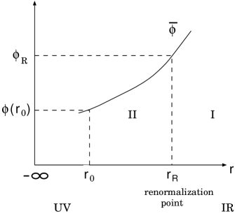
Figure 1: The evolution of the classical solutions $\bar{\phi}^{i}$ along the radial direction. The region I is defined by $r\geq r_{R}$, and the region II is defined by $r_{0}\leq r<r_{R}$.

That is, if we would like to fix the couplings at the “renormalization point” $r=r_{R}$ to be $G_{R}(x)$ and $\phi_{R}(x)$ and to require that physics does not change as the cutoff moves, we only need to take the bare sources to be

$$G_{\mu\nu}(x,r_{0})=\overline{G}_{\mu\nu}(x,r_{0};G_{R},r_{R}),\qquad\phi^{i}(x,r_{0})=\bar{\phi}^{i}(x,r_{0};\phi_{R},r_{R}).$$ (4.3)

The on-shell action with these running bare sources can be easily evaluated by using Eq. (4.3):

$$S[G_{\mu\nu}(x,r_{0}),\,\phi^{i}(x,r_{0})]\!\!\! = \!\!\!\int d^{d}x\int_{r_{0}}dr\,\sqrt{\overline{G}}\,{\cal L}_{d+1}\left[\overline{G}(x,r;G_{R},r_{R}),\bar{\phi}(x,r;\phi_{R},r_{R})\right]$$ (4.4)

$$= \!\!\!\int d^{d}x\left(\int_{r_{R}}dr+\int_{r_{0}}^{r_{R}}dr\right)\sqrt{\overline{G}}\,{\cal L}_{d+1}$$

$$= \!\!\!\ S_{R}[G_{R}(x),\phi_{R}(x)]+S_{\rm CT}\left[G_{R}(x),\phi_{R}(x);r_{0},r_{R}\right].$$

Here $S_{R}$ is given by integrating $\sqrt{\overline{G}}{\cal L}_{d+1}$ over the region I in Fig. 1, and it obeys the Hamiltonian constraint, which ensures that $S_{R}$ does not depend on $r_{R}$. On the other hand, $S_{\rm CT}$ is given by integrating $\sqrt{\overline{G}}{\cal L}_{d+1}$ over the region II. It also obeys the Hamiltonian constraint and thus does not depend on the coordinates of the boundaries of integration, $r_{R}$ and $r_{0}$, explicitly. However, in this case, their dependence implicitly enters $S_{\rm CT}$ through the condition that the boundary values at $r=r_{0}$ are on the classical trajectory through the renormalization point:

$$S_{{\rm CT}} = S\left[G_{R}(x),\phi_{R}(x);G(x,r_{0}),\phi(x,r_{0})\right]$$ (4.5)

$$= S\left[G_{R}(x),\phi_{R}(x);\overline{G}(x,r_{0};G_{R},r_{R}),\bar{\phi}(x,r_{0};\phi_{R},r_{R})\right].$$

It is thus natural to interpret $S_{\rm CT}[G_{R},\phi_{R};r_{0},r_{R}]$ as the counterterm, and the nonlocal part of $S_{R}[G_{R},\phi_{R}]$ gives the renormalized generating functional of the boundary field theory, $\Gamma_{R}[G_{R},\phi_{R}]$, written in terms of the renormalized sources.

Since, as pointed out above, $S_{R}[G_{R},\phi_{R}]$ also satisfies the Hamiltonian constraint, it will yield the same form of the flow equation, with all the bare fields replaced by the renormalized fields. This suggests that the holographic RG exactly describes the so-called renormalized trajectory [16], which is a submanifold in the parameter space, consisting of the flows driven by relevant perturbations from an RG fixed point at $r_{0}=-\infty$.

5 Relation to the analysis by Henningson and Skenderis

In this section, we comment on the relation between the analysis given above and that of Henningson and Skenderis [13], which is briefly reviewed in Appendix D. In particular, we show that ${S_{\rm loc}}$, the local part of the on-shell action, can also be calculated solely from their analysis. In the following discussion, we exclusively consider the pure gravity case. Extension to the case in which matter fields exist should be straightforward.

First, we recall that in our analysis, the bare coupling $G(x)$ at $r=r_{0}$ is tuned in such a way that it is on the classical trajectory that passes through a fixed value $G_{R}$ at some renormalization point, $r=r_{R}$ (see Eq. (4.3)):

$$G(x)\rightarrow G(x,r_{0})=\overline{G}(x,r_{0};G_{R},r_{R}).$$ (5.1)

The value $G_{R}$ is regarded as the renormalized coupling at $r=r_{R}$. On the other hand, it is also possible to choose as the renormalized coupling the coefficient of the asymptotic form of the classical solution, as is done in Ref. [13]. That is, by expanding the classical solution in the limit $r\rightarrow-\infty$,

$$\overline{G}_{\mu\nu}(x,r)=e^{-2r}\left(g^{(0)}_{\mu\nu}(x)+e^{2r}g^{(2)}_{\mu\nu}(x)+\cdots\right),$$ (5.2)

one can interpret $g_{(0)}$ as the renormalized coupling. Here $g_{(2)},g_{(4)},\cdots$ are obtained as local functions constructed from $g_{(0)}$ in such a way that $\overline{G}(x,r)$ satisfies the equation of motion. Some of them are given explicitly in Appendix D. The two renormalized couplings, $G_{R}(x)$ and $g_{(0)}(x)$, are related through the simple relation

$$G(x,r_{0}) = \overline{G}(x,r_{0};G_{R},r_{R})$$ (5.3)

$$= e^{-2r_{0}}\left(g_{(0)}(x)+e^{2r_{0}}g_{(2)}\!\left[g_{(0)}(x)\right]+e^{4r_{0}}g_{(4)}\!\left[g_{(0)}(x)\right]+\cdots\right).$$

Now we show that once the counterterm is known within the scheme of Henningson and Skenderis, we can directly calculate the local part of the on-shell action, ${S_{\rm loc}}[G]$. To show this, we first introduce the new coordinate $\rho\equiv e^{2r}$ and set $\epsilon\equiv e^{2r_{0}}$. The classical solution is thus expanded around $\rho=0$ as (see Appendix D)

$$\overline{G}(x,\rho)\!\!\! = \!\!\!\frac{1}{\rho}\,\Biggl{[}g_{(0)}(x)+\rho\,g_{(2)}\!\left[g_{(0)}(x)\right]+\cdots+\rho^{d/2}\left(g_{(d)}\!\left[g_{(0)}(x)\right]+\log\rho\,h_{(d)}\!\left[g_{(0)}(x)\right]\right)+\cdots\Biggr{]}.$$

We then require that this classical solution passes through the point $\widehat{g}(x)/\epsilon$ at $\rho=\epsilon$ (see Fig. 2) with $\widehat{g}(x)$ some fixed function:

$$\frac{1}{\epsilon}\,\widehat{g}(x)\equiv\overline{G}(x,\epsilon)=\frac{1}{\epsilon}\,\left(g_{(0)}(x)+\epsilon\,g_{(2)}\!\left[g_{(0)}(x)\right]+\cdots\right).$$ (5.5)

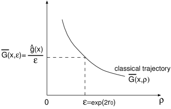
Figure 2: The classical solution $\overline{G}(x,\rho)$ with $\rho=\exp(2r)$ is chosen such that it passes through the point $\widehat{g}(x)/\epsilon$ at $\rho=\epsilon$ (i.e., $r=r_{0}$).

This can be solved recursively as

$$g_{(0)}\!\left[\widehat{g}(x),\epsilon\right]=\widehat{g}(x)+\epsilon\,b_{(2)}\!\left[\widehat{g}(x)\right]+\cdots+\epsilon^{d/2}\,\left(b_{(d)}\!\left[\widehat{g}(x)\right]+\log\epsilon\,c_{(d)}\!\left[\widehat{g}(x)\right]\right)+\cdots.$$ (5.6)

Since $G=\widehat{g}/\epsilon$ is the boundary value of the classical solution at $\rho=\epsilon$ (i.e., $r=r_{0}$), we have

$$S\left[\widehat{g}(x)/\epsilon\right]=S_{d+1}\left[\overline{G}\left(x,r;\,\widehat{g}/\epsilon,r_{0}\right)\right].$$ (5.7)

The right-hand side is identical to the on-shell action in the scheme of Henningson and Skenderis given in Appendix D, with $g_{(0)}=g_{(0)}[\widehat{g},\epsilon]$. We thus have

$$S[\widehat{g}/\epsilon]=S^{\rm HS}\left[g_{(0)}[\widehat{g},\epsilon],\epsilon\right].$$ (5.8)

We can then extract the terms that diverge in the limit $\epsilon\rightarrow 0$ as follows. We first note that $S[\widehat{g}/\epsilon]$ can be written as

$$S[\widehat{g}/\epsilon]={S_{\rm loc}}[\widehat{g}/\epsilon]+\Gamma[\widehat{g}/\epsilon].$$ (5.9)

Here ${S_{\rm loc}}[\widehat{g}/\epsilon]$ is a meromorphic function of $\epsilon$ and has the following Laurent expansion:

$$S_{\rm loc}[\widehat{g}/\epsilon]=\sum_{w=0,2,4,\cdots}\epsilon^{(w-d)/2}\int d^{d}x\sqrt{\widehat{g}}\Bigl{[}{\cal L}_{\rm loc}[\widehat{g}]\Bigr{]}_{w}.$$ (5.10)

$\Gamma[\widehat{g}/\epsilon]$, on the other hand, may lead to a logarithmically divergent term. We thus obtain the following equation for the divergent terms:

$$\sum_{w=0}^{d-2}\epsilon^{(w-d)/2}\int d^{d}x\,\sqrt{\widehat{g}}\,\Bigl{[}{\cal L}_{\rm loc}[\widehat{g}]\Bigr{]}_{w}-\log\epsilon\,\int d^{d}x\,\sqrt{\widehat{g}}\,\,\widehat{{\cal W}}_{d}\,=\,S^{\rm HS}_{\rm div}\left[g_{(0)}[\widehat{g},\epsilon],\,\epsilon\right].$$ (5.11)

The quantity $S^{\rm HS}_{\rm div}\left[g_{(0)}[\widehat{g},\epsilon],\,\epsilon\right]$, the divergent part of $S^{\rm HS}$, is calculated in Ref. [13] (see also Appendix D). By considering the structure, one can easily understand that $\widehat{{\cal W}}_{d}$ should be the Weyl anomaly written in terms of $\widehat{g}$. Equation (5.11) shows that the relevant part of ${S_{\rm loc}}$ can be calculated from the divergent term of $S^{\rm HS}$ by comparing terms of the same order in $\epsilon$.

We now give sample calculations for $d=4$ and $d=6$.

$d=4$:

Straightforward calculation gives the coefficients $b_{(2)},\cdots$ as

$$\begin{array}[]{cclcl}b_{(2)}&=&-\widehat{g}_{(2)}&&\left(\widehat{g}_{(2)}\equiv g_{(2)}[\widehat{g}]\right),\\ b_{(4)}&=&-\widehat{D}-\widehat{g}_{(4)}&&\left(\widehat{g}_{(4)}\equiv g_{(4)}[\widehat{g}]\right),\\ c_{(4)}&=&-\widehat{h}_{(4)}&&\left(\widehat{h}_{(4)}\equiv h_{(4)}[\widehat{g}]\right),\end{array}$$ (5.15)

where $\widehat{D}_{\mu\nu}$ is the covariant tensor given by

$$\widehat{D}_{\mu\nu} = {1\over 4}\left[\,\widehat{\nabla}^{\sigma}\left(\widehat{\nabla}_{\mu}\widehat{g}^{(2)}_{\nu\sigma}+\widehat{\nabla}_{\nu}\widehat{g}^{(2)}_{\mu\sigma}\right)-\widehat{\nabla}^{2}\widehat{g}^{(2)}_{\mu\nu}-\widehat{\nabla}_{\mu}\widehat{\nabla}_{\nu}{\rm tr}(\widehat{g}^{-1}\widehat{g}_{(2)})\,\right]$$

$$~{}-{1\over 12}\left[\,-\widehat{g}^{(2)}_{\lambda\sigma}\widehat{R}^{\lambda\sigma}+\widehat{\nabla}^{\lambda}\widehat{\nabla}^{\sigma}\widehat{g}^{(2)}_{\lambda\sigma}-\widehat{\nabla}^{2}{\rm tr}(\widehat{g}^{-1}\widehat{g}_{(2)})\,\right]\widehat{g}_{\mu\nu}-{1\over 12}\,\widehat{R}\,\widehat{g}^{(2)}_{\mu\nu}.$$

Substituting these values into Eq. (D.11), we obtain

$$S_{\rm div}^{\rm HS}\left[g_{(0)}[\widehat{g}(x),\epsilon],\epsilon\right]=\int d^{4}x\sqrt{\widehat{g}}\left(-{6\over\epsilon^{2}}-{1\over 2\epsilon}\widehat{R}-\log\epsilon\,\,\widehat{{\cal W}}_{4}\right).$$ (5.17)

This actually gives Eqs. (3.30) and (3.31) with $\phi=0$ and $l=1$.

$d=6$:

The coefficients are calculated to be

$$b^{(2)}_{\mu\nu} = {1\over 4}\left(\widehat{R}_{\mu\nu}-{1\over 10}\widehat{R}\widehat{g}_{\mu\nu}\right),$$

$$b^{(4)}_{\mu\nu} = {1\over 16}\widehat{R}^{\lambda\sigma}\widehat{R}_{\mu\lambda\nu\sigma}-{1\over 32}\widehat{R}_{\mu}^{\lambda}\widehat{R}_{\lambda\nu}-{1\over 80}\widehat{R}\widehat{R}_{\mu\nu}-{9\over 640}\widehat{g}_{\mu\nu}\widehat{R}^{\lambda\sigma}\widehat{R}_{\lambda\sigma}+{9\over 4^{4}5^{2}}\widehat{R}^{2}\,\widehat{g}_{\mu\nu},$$

which lead to

$$S^{\rm HS}_{\rm div}\left[g_{(0)}[\widehat{g}(x),\epsilon],\epsilon\right]\!\!\! = \!\!\!\int d^{6}x\sqrt{\widehat{g}}\left(-{10\over\epsilon^{3}}-{1\over 4\epsilon^{2}}\widehat{R}+{3\over 320\epsilon}\widehat{R}^{2}-{1\over 32\epsilon}\widehat{R}_{\mu\nu}\widehat{R}^{\mu\nu}-\log\epsilon\,\,\widehat{{\cal W}}_{6}\right).$$

This reproduces Eqs. (3.32) and (3.33) with $l=1$.

6 Conclusion

In this note, we have discussed several aspects of the holographic RG that are related to the Weyl anomaly. We found that the Hamilton-Jacobi constraint is quite useful in exploring the holographic RG, especially to calculate the Weyl anomaly and to understand the structure of divergent parts. We also discussed continuum limits of the boundary theories in the context of the holographic RG. In particular we demonstrated that counterterms can be extracted systematically if we use a special renormalization, where the bare and the renormalized couplings are on the same classical trajectories determined by the bulk theory. Finally, we discussed the relationship between the present formalism and the analysis of Henningson and Skenderis, and found an algorithm determining the local part of the on-shell action, ${S_{\rm loc}}[G(x),\phi(x)]$, from the divergent terms in their calculation.

Appendix A Variations of Curvature

In this appendix, we list the variations of the curvature tensor, Ricci tensor and Ricci scalar with respect to the metric.

Our convention is

$$R^{\mu}_{~{}\,\nu\lambda\sigma} \equiv \partial_{\lambda}\Gamma_{\sigma\nu}^{\mu}+\Gamma_{\lambda\rho}^{\mu}\Gamma_{\sigma\nu}^{\rho}-(\lambda\leftrightarrow\sigma),$$

$$R_{\mu\nu} \equiv R^{\rho}_{~{}\mu\rho\nu},\qquad R\,\equiv\,G^{\mu\nu}\,R_{\mu\nu}.$$ (A.1)

The fundamental formula is

$$\delta\Gamma^{\kappa}_{\mu\nu}=\frac{1}{2}\,G^{\kappa\lambda}\,\left(\nabla_{\mu}\,\delta G_{\nu\lambda}+\nabla_{\nu}\,\delta G_{\mu\lambda}-\nabla_{\lambda}\,\delta G_{\mu\nu}\right),$$ (A.2)

from which one can calculate the variations of curvatures:

$$\delta R^{\mu}_{~{}\,\nu\lambda\sigma} = \nabla_{\lambda}\,\delta\Gamma^{\mu}_{\sigma\nu}-\nabla_{\sigma}\,\delta\Gamma^{\mu}_{\lambda\nu},$$ (A.3)

$$\delta R_{\mu\nu\lambda\sigma} = \frac{1}{2}\Bigl{[}\nabla_{\lambda}\nabla_{\nu}\delta G_{\sigma\mu}-\nabla_{\lambda}\nabla_{\mu}\delta G_{\sigma\nu}-\nabla_{\sigma}\nabla_{\nu}\delta G_{\lambda\mu}+\nabla_{\sigma}\nabla_{\mu}\delta G_{\lambda\nu}$$ (A.4)

$$~{}~{}+\delta G_{\mu\rho}\,R^{\rho}_{~{}\nu\lambda\sigma}-\delta G_{\nu\rho}\,R^{\rho}_{~{}\mu\lambda\sigma}\Bigr{]},$$

$$\delta R_{\mu\nu} = \frac{1}{2}\left[\nabla^{\rho}\left(\nabla_{\mu}\delta G_{\nu\rho}+\nabla_{\nu}\delta G_{\mu\rho}\right)-\nabla^{2}\delta G_{\mu\nu}-\nabla_{\mu}\nabla_{\nu}\left(G^{\rho\lambda}\delta G_{\rho\lambda}\right)\right],$$

$$\delta R = -\delta G_{\mu\nu}\,R^{\mu\nu}+\nabla^{\mu}\nabla^{\nu}\delta G_{\mu\nu}-\nabla^{2}\left(G^{\mu\nu}\delta G_{\mu\nu}\right).$$ (A.6)

Here note that

$$\Bigl{[}\nabla_{\mu},\nabla_{\nu}\Bigr{]}\,\delta G_{\lambda\sigma}=-\delta G_{\rho\sigma}\,R^{\rho}_{~{}\lambda\mu\nu}-\delta G_{\lambda\rho}\,R^{\rho}_{~{}\sigma\mu\nu}.$$ (A.7)

Appendix B Variations of $S_{\rm loc}[G(x),\phi(x)]$

In this appendix, we list the variations of $S_{\rm loc}[G(x),\phi(x)]$.

Pure gravity:

If we only consider terms with weight $w\leq 4$ of the form

$$S_{\rm loc}[G]=\int d^{d}x\sqrt{G}\left(W-\Phi R+XR^{2}+YR_{\mu\nu}R^{\mu\nu}+ZR_{\mu\nu\rho\lambda}R^{\mu\nu\rho\lambda}\right),$$ (B.1)

then we have

$$\frac{1}{\sqrt{G}}\frac{\delta S_{\rm loc}}{\delta G_{\mu\nu}}\!\! = \!\!\frac{1}{2}\Bigl{(}W-\Phi R+XR^{2}+YR_{\mu\nu}R^{\mu\nu}+ZR_{\mu\nu\rho\lambda}R^{\mu\nu\rho\lambda}\Bigr{)}G^{\mu\nu}$$ (B.2)

$$+\,\Phi R^{\mu\nu}-2X\Bigl{(}RR^{\mu\nu}-\nabla^{\mu}\nabla^{\nu}R\Bigr{)}-Y\Bigl{(}2R^{\mu}_{\,~{}\rho}R^{\nu\rho}-2\nabla_{\rho}\nabla^{\left(\mu\right.}R^{\left.\nu\right)\rho}+\nabla^{2}R^{\mu\nu}\Bigr{)}$$

$$-2Z\Bigl{(}R^{\mu}_{~{}\,\rho\lambda\sigma}R^{\nu\rho\lambda\sigma}-2\nabla^{\rho}\nabla^{\lambda}R^{\left(\mu~{}~{}\nu\right)}_{~{}~{}\rho\lambda~{}}\Bigr{)}-\left(2X+\frac{1}{2}\,Y\right)G^{\mu\nu}\,\nabla^{2}R,$$

and thus

$$\frac{1}{\sqrt{G}}\,G_{\mu\nu}\,\frac{\delta S_{\rm loc}}{\delta G_{\mu\nu}} = \frac{d}{2}\,W-\frac{d-2}{2}\,\Phi\,R+\frac{d-4}{2}\left(XR^{2}+YR_{\mu\nu}R^{\mu\nu}+ZR_{\mu\nu\rho\lambda}R^{\mu\nu\rho\lambda}\right)$$ (B.3)

$$~{}-\left(2(d-1)X+\frac{d}{2}\,Y+2Z\right)\nabla^{2}R.$$

In the last expression, we have used the Bianchi identity: $\nabla^{\mu}R_{\mu\nu}=(1/2)\nabla_{\nu}R$.

Gravity coupled to scalars:

For $S_{\rm loc}[G,\phi]$ of the form

$$S_{\rm loc}[G,\phi]=\int d^{d}x\sqrt{G}\left(W(\phi)-\Phi(\phi)R+\frac{1}{2}M_{ij}(\phi)G^{\mu\nu}\partial_{\mu}\phi^{i}\partial_{\nu}\phi^{j}\right),$$ (B.4)

we have

$$\frac{1}{\sqrt{G}}\frac{\delta{S_{\rm loc}}}{\delta G_{\mu\nu}} = \frac{1}{2}\left(W-\Phi R+\frac{1}{2}\,M_{ij}\,\partial_{\rho}\phi^{i}\,\partial^{\rho}\phi^{j}\right)G^{\mu\nu}$$ (B.5)

$$+\,\Phi\,R^{\mu\nu}+G^{\mu\nu}\,\nabla^{2}\Phi-\nabla^{\mu}\nabla^{\nu}\Phi-\frac{1}{2}\,M_{ij}\,\partial^{\mu}\phi^{i}\,\partial^{\nu}\phi^{j},$$

$$\frac{1}{\sqrt{G}}\frac{\delta{S_{\rm loc}}}{\delta\phi^{i}} = \partial_{i}W-\partial_{i}\Phi\,R-M_{ij}\,\nabla^{2}\phi^{j}-\Gamma_{i;jk}^{(M)}\,\partial_{\mu}\phi^{j}\,\partial^{\mu}\phi^{k},$$ (B.6)

where $\Gamma_{jk}^{(M)i}(\phi)\equiv M^{il}(\phi)\,\Gamma_{l;jk}^{(M)}(\phi)$ is the Christoffel symbol constructed from $M_{ij}(\phi)$.

Appendix C RG Flow and the Classical Solutions in the Bulk

According to the holographic RG, the RG flow in the boundary field theory should be described by the classical solutions in the bulk. Although this is clearly explained for $d=4$ in Ref. [12], we repeat their argument for arbitrary dimensions, in order to make our discussion self-contained. To this end, we start with the classical solutions $\overline{G}_{\mu\nu}(x,r;G(x),r_{0})$ and $\bar{\phi}^{i}(x,r;\phi(x),r_{0})$ with the boundary conditions

$$\overline{G}_{\mu\nu}(x,r_{0})=G_{\mu\nu}(x)\equiv{1\over a^{2}}\,\delta_{\mu\nu},\qquad\bar{\phi}^{i}(x,r_{0})=\phi^{i}(x)\equiv\phi^{i}={\rm const.}$$ (C.1)

Since we set the fields to constant values, the system is now perturbed finitely. Furthermore, since $a$ gives the unit length of the metric $G_{\mu\nu}(x)$, this perturbation should describe the system with the cutoff length $a$, which corresponds to the time $r=r_{0}$ in the RG flow. From Eq. (2.7) and the Hamilton-Jacobi equation (2.13), we obtain

$${d\over dr}\overline{G}_{\mu\nu}(x,r;G,r_{0})\Bigg{|}_{r=r_{0}} = {1\over d-1}\,W(\phi)\,{1\over a^{2}}\,\delta_{\mu\nu},$$ (C.2)

$${d\over dr}\bar{\phi}^{i}(x,r;\phi,r_{0})\Big{|}_{r=r_{0}} = -L^{ij}(\phi)\,\partial_{j}W(\phi).$$ (C.3)

We then assume that the classical solutions take the following form for general $r$:

$$\overline{G}_{\mu\nu}(x,r;G,r_{0})={1\over a(r)^{2}}\delta_{\mu\nu},\qquad\bar{\phi}^{i}(x,r;\phi,r_{0})=\phi^{i}(a(r)),$$ (C.4)

with $a(r_{0})=a$. Note that $a(r)$ can be identified with the cutoff length at $r$. It then follows from (C.2) and (C.3) that

$$a\,{dr\over da} = -\,{2(d-1)\over W(\phi)},$$ (C.5)

$$a\,{d\over da}\,\phi^{i}(a) = {2(d-1)\over W(\phi)}\,L^{ij}(\phi)\,\partial_{j}W(\phi).$$ (C.6)

The latter agrees with the beta function in Eq. (3.25).

Appendix D Analysis of the Weyl Anomaly à la Henningson and Skenderis

It is convenient to introduce the coordinate $\rho\equiv e^{2r}$ and rewrite the metric in the following way, as in Ref. [13]:

$$ds^{2}={d\rho^{2}\over 4\rho^{2}}+{g_{\mu\nu}(x,\rho)\over\rho}\,dx^{\mu}dx^{\nu}.$$ (D.1)

The metric $g_{\mu\nu}(x,\rho)$ is related to our metric, $G_{\mu\nu}(x,r)$, as

$$G_{\mu\nu}(x,r)={g_{\mu\nu}(x,\rho)\over\rho}\qquad\left(\,\rho=e^{2r}\,\right).$$ (D.2)

Assuming the existence of an asymptotically AdS_d+1 boundary at $\rho=0$, we expand the metric as

$$g(x,\rho)=g_{(0)}(x)+\rho\,g_{(2)}(x)+\cdots+\rho^{d/2}\left(g_{(d)}(x)+\log\rho~{}h_{(d)}(x)\right)+O(\rho^{d/2+1}).$$ (D.3)

Then the equations of motion for $g_{\mu\nu}$,

$$0 = {\rm tr}(g^{-1}g^{\prime\prime})-\frac{1}{2}{\rm tr}(g^{-1}g^{\prime}g^{-1}g^{\prime}),$$ (D.4)

$$0 = \nabla^{\nu}g^{\prime}_{\mu\nu}-\partial_{\mu}{\rm tr}(g^{-1}g^{\prime}),$$ (D.5)

$$0 = -{\rm Ric}(g)+\rho\left[2g^{\prime\prime}-2g^{\prime}g^{-1}g^{\prime}+{\rm tr}(g^{-1}g^{\prime})g^{\prime}\right]-(d-2)g^{\prime}-{\rm tr}(g^{-1}g^{\prime})g,$$

can be solved iteratively for small $\rho$, giving the coefficient functions $g_{(2)},g_{(4)},\cdots$ as functions of $g_{(0)}$ [13] (see also Ref. [22]). Here $\nabla_{\mu}$ is the covariant derivative with respect to $g_{\mu\nu}$, and the prime represents $\partial/\partial\rho$. The tensors $g_{(k)}~{}(k=0,2,\cdots,d-2)$ and $h_{(d)}$ are obtained as covariant expressions with respect to $g_{(0)}$. Although ${\rm tr}\left(g_{(0)}^{-1}g_{(d)}\right)$ is an invariant scalar, $g_{(d)}$ itself cannot be expressed covariantly. The quantity ${\rm tr}\left(g_{(0)}^{-1}h_{(d)}\right)$ turns out to vanish identically. Then, substituting the classical solution into the bulk action, we can explicitly evaluate the dependence of the on-shell action on the coordinate of the boundary, $\rho\equiv\epsilon$:

$$S^{\rm HS}[g_{(0)},\epsilon]=\int d^{d}x\left[\,d\int_{\epsilon}d\rho\,\sqrt{g}\,\rho^{-d/2-1}+\left(4\rho^{-d/2+1}\sqrt{g}^{\,\prime}-2\,d\,\rho^{-d/2}\sqrt{g}\right)\Bigg{|}_{\rho=\epsilon}\right].$$ (D.7)

$d=4$:

The coefficients necessary for the calculation are (using the convention described in Appendix A)

$$g_{(2)} = -{1\over 2}\left({\rm Ric}(g_{(0)})-{1\over 6}R(g_{(0)})g_{(0)}\right),$$ (D.8)

$${\rm tr}\left[g_{(0)}^{-1}g_{(4)}\right] = {1\over 16}\left(R^{\mu\nu}(g_{(0)})R_{\mu\nu}(g_{(0)})-{2\over 9}(R(g_{(0)}))^{2}\right),$$ (D.9)

$$4h_{(4)} = 2g_{(2)}g_{(0)}^{-1}g_{(2)}+{\rm Ric}^{\prime}(g)|_{\rho=0}+{\rm tr}\left(2g_{(0)}^{-1}g_{(4)}-g_{(0)}^{-1}g_{(2)}g_{(0)}^{-1}g_{(2)}\right)g_{(0)}.$$

The on-shell action is thus evaluated as

$$S^{\rm HS}[g_{(0)},\epsilon]=\int d^{4}x\sqrt{g_{(0)}}\left(-{6\over\epsilon^{2}}+{3\over\epsilon}R(g_{(0)})-\log\epsilon\,\,{\cal W}_{4}[g_{(0)}]\right)+\Gamma^{\rm HS}_{\rm fin}[g_{(0)},\epsilon].$$

(D.11)

Here ${\cal W}_{d}[g_{(0)}]$ is the $d$-dimensional Weyl anomaly written in terms of $g_{(0)}$, and $\Gamma^{\rm HS}_{\rm fin}[g_{(0)},\epsilon]$ is the finite part in the limit $\epsilon\rightarrow 0$.

$d=6$:

The calculation is completely parallel to that for the $d=4$ case, and we find

$$g_{(2)} = -\frac{1}{4}\left({\rm Ric}(g_{(0)})-\frac{1}{10}Rg_{(0)}\right),$$ (D.12)

$${\rm tr}\left[g_{(0)}^{-1}g_{(4)}\right] = \frac{1}{64}{\rm tr}\left({\rm Ric}(g_{(0)})^{2}\right)-\frac{7}{3200}R(g_{(0)})^{2},$$ (D.13)

$${\rm tr}[g_{(0)}^{-1}g_{(2)}g_{(0)}^{-1}g_{(2)}] = \frac{1}{16}{\rm tr}\left({\rm Ric}(g_{(0)})^{2}\right)-\frac{7}{800}R(g_{(0)})^{2},$$ (D.14)

from which we calculate

$$S^{\rm HS}[g_{(0)},\epsilon]=\int d^{6}x\sqrt{g_{(0)}}\left(-{10\over\epsilon^{3}}+{1\over 4\epsilon^{2}}R+{3\over 640\epsilon}R^{2}-{1\over 64\epsilon}R_{\mu\nu}R^{\mu\nu}-\log\epsilon\,\,{\cal W}_{6}[g_{(0)}]\right)$$

$$~{}~{}~{}~{}~{}~{}~{}~{}~{}~{}~{}~{}~{}~{}~{}~{}~{}~{}~{}~{}+\Gamma^{\rm HS}_{\rm fin}[g_{(0)},\epsilon].$$ (D.15)

Since the metric appears in the bulk action only through the combination $G_{\mu\nu}(x,r)=g_{\mu\nu}(x,\rho)/\rho$, we obtain the relation

$$S^{\rm HS}[e^{2\sigma}g_{(0)},e^{2\sigma}\epsilon]=S^{\rm HS}[g_{(0)},\epsilon],$$ (D.16)

which implies that the coefficient of $\log\epsilon$ actually gives the anomaly

$$\Gamma^{\rm HS}_{R}[e^{2\sigma}g_{(0)}]-\Gamma^{\rm HS}_{R}[g_{(0)}]=2\int d^{d}x\sqrt{g_{(0)}}\,\,{\cal W}_{d}[g_{(0)}]\,\sigma~{}~{}~{}(\sigma\ll 1).$$ (D.17)

where $\Gamma^{\rm HS}_{R}[g_{(0)}]\equiv\lim_{\epsilon\rightarrow 0}\Gamma^{\rm HS}_{\rm fin}[g_{(0)},\epsilon]$. Note also that Eq. (D.16) implies that $S^{\rm HS}[g_{(0)},\epsilon]$ depends only on $g_{(0)}/\epsilon$.

References

[1]
J. Maldacena,
“The large limit of superconformal field theories and
supergravity,”
Adv. Theor. Math. Phys. 2 (1998) 231,
hep-th/9711200; S. S. Gubser, I. R. Klebanov and A. M. Polyakov,
“Gauge Theory Correlators from Non-Critical String Theory,”
Phys. Lett. B428 (1998) 105,
hep-th/9802109; E. Witten,
“Anti De Sitter Space And Holography,”
Adv. Theor. Math. Phys. 2 (1998) 253,
hep-th/9802150.
[2]
O. Aharony, S. S. Gubser, J. Maldacena, H. Ooguri and Y. Oz,
“Large N Field Theories, String Theory and Gravity,”
hep-th/9905111, and references therein.
[3]
E. T. Akhmedov,
“A remark on the AdS/CFT correspondence and the renormalization
group flow,”
Phys. Lett. B442 (1998) 152,
hep-th/9806217.
[4]
E. Alvarez and C. Gomez,
“Geometric Holography, the Renormalization Group
and the c-Theorem,”
Nucl. Phys. B541 (1999) 441,
hep-th/9807226.
[5]
D. Z. Freedman, S. S. Gubser, K. Pilch and N. P. Warner,
“Renormalization Group Flows from Holography–Supersymmetry
and a c-Theorem,”
hep-th/9904017.
[6]
L. Girardello, M. Petrini, M. Porrati and A. Zaffaroni,
“Novel Local CFT and Exact Results on Perturbations of N=4 Super
Yang Mills from AdS Dynamics,”
J. High Energy Phys. 12 (1998) 022,
hep-th/9810126.
[7]
L. Girardello, M. Petrini, M. Porrati and A. Zaffaroni
“The Supergravity Dual of N=1 Super Yang-Mills Theory,”
Nucl. Phys. B569 (2000) 451,
hep-th/9909047.
[8]
M. Porrati and A. Starinets,
“RG Fixed Points in Supergravity Duals of 4-d Field Theory and
Asymptotically AdS Spaces,”
Phys. Lett. B454 (1999) 77,
hep-th/9903085.
[9]
V. Balasubramanian and P. Kraus,
“Spacetime and the Holographic Renormalization Group,”
Phys. Rev. Lett. 83 (1999) 3605,
hep-th/9903190.
[10]
K. Skenderis and P. K. Townsend,
“Gravitational Stability and Renormalization-Group Flow,”
Phys. Lett. B468 (1999) 46,
hep-th/9909070.
[11]
O. DeWolfe, D. Z. Freedman, S. S. Gubser and A. Karch,
“Modeling the fifth dimension with scalars and gravity,”
hep-th/9909134.
[12]
J. de Boer, E. Verlinde and H. Verlinde,
“On the Holographic Renormalization Group,”
hep-th/9912012.
[13]
M. Henningson and K. Skenderis,
“The Holographic Weyl anomaly,”
J. High Energy Phys. 07 (1998) 023,
hep-th/9806087.
[14]
M. J. Duff,
“Twenty Years of the Weyl Anomaly,”
Class. Quant. Grav. 11 (1994) 1387,
hep-th/9308075.
[15]
S. Corley,
“A Note on Holographic Ward Identities,”
Phys. Lett. B484 (2000) 141,
hep-th/0004030.
[16]
K. Wilson and J. Kogut,
“The Renormalization Group and the -Expansion,”
Phys. Rep. 12 (1974) 75.
[17]
G. W. Gibbons and S. W. Hawking,
“Action Integrals and Partition Functions in Quantum Gravity,”
Phys. Rev. D15 (1977) 2752.
[18]
C. R. Graham and J. M. Lee, “Einstein Metrics with Prescribed
Conformal Infinity on the Ball,”
Adv. Math. 87 (1991) 186.
[19]
M. Green, J. Schwarz and E. Witten,
“Superstring Theory,” Cambridge University Press, New York, 1987.
[20]
S. Nojiri and S. Odintsov,
“Conformal Anomaly for Dilaton Coupled Theories from
AdS/CFT Correspondence,”
Phys. Lett. B444 (1998) 92,
hep-th/9810008; S. Nojiri, S. Odintsov and S. Ogushi,
“Conformal Anomaly from d5 Gauged Supergravity and c-function
Away from Conformity,”
hep-th/9912191;
“Finite Action in d5 Gauged Supergravity and Dilatonic Conformal
Anomaly for Dual Quantum Field Theory,”
hep-th/0001122.
[21]
V. Balasubramanian and P. Kraus,
“Spacetime and the Holographic Renormalization Group,”
Commun. Math. Phys. 208 (1999) 413, hep-th/9902121.
[22]
S. de Haro, K. Skenderis and S. Solodukhin,
“Holographic Reconstruction of Spacetime
and Renormalization in the AdS/CFT Correspondence,”
hep-th/0002230.