TSU HEPI 2000-04

1 Introduction

The main aim of this article is to demonstrate that equations of the relativistic quantum theory may have solutions which have no nonrelativstic analogue. Some of such solutions are well-known, e.g. the so-called abnormal solutions. Nakanishi wrote about the latters: ”The non-relativistic common sense does not necessarily remain valid in the relativistic quantum field theory” [1].

The main ideas of this article were published as a preprint of Tbilisi Mathematical Institute in collaboration with A. Tavkhelidze and L. Vachnadze [2].

At first the interest to the problem was initiated by the observed narrow peaks around $1.5MeV$ in the $e^{+}e^{-}$ distribution in the experiments of heavy ion collisions [3] . These resonances are known as the GSI resonances. They are situated above the $2m_{e}$ threshold and it naturally triggered interest to studies of bound states in continuum. In the papers of the Serpukhov and other groups [5] the single-photon exchange quasipotential equations in QED were studied and, relying on the numeric methods, large number of peaks were reported.

The quasipotential equation can be obtained from the Bethe-Salpeter equation after certain approximation. So it was natural to try to cope with the same problem within the framework of the ladder approximation of the Bethe-Salpeter equation itself. It was particularly interesting because there was no such observation made on the earlier stages of studies of the Bethe-Salpeter (BS) equation (for a review see [1]). However, we think that nobody has searched for bound states in the continuum there. It is worth noting that when the total mass $M>2m$ the traditional method — Wick’s rotation is, in general, inadmissible. So the problem must be considered in the Minkowski space. Structure of the ladder BS equation for this case was studied by Günter [7] and it was demonstrated that Wick’s rotation is inadmissible. In the recent years interest to the BS equations in the Minkowski space has increased [8],[9]. Below, employing standard methods, we will reduce the BS equation to the system of the one-dimensional equations and study unusual solutions in the continuous spectrum. Note that though further experiments have not confirmed existence of the GSI resonances the possibility of bound states embedded in the continuum is interesting on its own.

2 Bethe-Salpeter equation in the Ladder approximation and its reduction

We will consider the BS equation in the ladder approximation for a simple model [6],[10] of two equal mass ($m$) scalar particles exchanging massless scalar meson, the so called Wick-Cutkosky model with the interaction Lagrangian:

$$L_{int}=g_{1}\phi_{1}^{*}\phi_{2}A+g_{2}\phi_{2}^{*}\phi_{1}A.$$

Standard equation has the form (in the rest frame):

$$\psi(p)=-\frac{\lambda}{\pi^{2}i}\int d^{4}q\frac{\psi(q)}{\left[\left(p-q\right)^{2}+io\right]\left[\left(\frac{P}{2}-q\right)^{2}-m^{2}\right]\left[\left(\frac{P}{2}+q\right)^{2}-m^{2}\right]}.$$ (1)

Here $P=p_{1}+p_{2}$ is the total 4-momentum, $p=\frac{1}{2}(p_{1}-p_{2})$ and $q$ are relative 4-momenta, $\lambda=\frac{g_{1}g_{2}}{(4\pi)^{2}}$ is the product of appropriate coupling constants and has dimension of the mass squared. In the rest frame where $\vec{P}=0$ and $\vec{p}_{1}=-\vec{p}_{2}=\vec{p}$ we will use the following notation for the total energy (mass) $P_{0}=E=M=2W$.

Usually the Wick-Cutkosky model is considered as an auxiliary (fictitious) one. But in some reasonable approximation more realistic models reduce to the Wick-Cutkosky one. Indeed, in the single-photon (gluon) approximation in QED (QCD) for fermion and antifermion bound state BS amplitude we have an equation:

$$\left[m-\gamma(\frac{P}{2}+p)\right]\psi(p)\left[m+\gamma(\frac{P}{2}-p)\right]==\frac{\lambda_{F}}{\pi^{2}i}\int d^{4}q\frac{\gamma_{\mu}\psi(q)\gamma_{\mu}}{(p-q)^{2}+io}$$

where $\lambda_{F}\equiv\left(\frac{g}{4\pi}\right)^{2}$ and the Feynman gauge is used.

Usually a new function

$$\Psi(p)=\left[m-\gamma(\frac{P}{2}+p)\right]\psi(p)\left[m+\gamma(\frac{P}{2}-p)\right]$$

is introduced [1] and the decomposition into the Dirac structures is considered:

$$\Psi=\Psi^{S}-\gamma_{5}\Psi^{P}+\gamma^{\mu}\Psi^{V}_{\mu}-\gamma^{\mu}\gamma_{5}\Psi^{A}_{\mu}-\frac{1}{2}[\gamma^{\mu},\gamma^{\nu}]\Psi_{\mu\nu}^{T}$$

Further one can obtain a chain of coupled equations for Dirac structures which can be considerably simplified by taking binding energies small (i.e. for weakly coupled system). All the components of $\Psi$ that survive in that limit of small binding energies ($\Psi^{P},\ \Psi^{A}_{\mu},\ \Psi^{V}$) satisfy the same equations:

$$\Psi^{i}(p)==-\frac{4\lambda_{F}m^{2}}{\pi^{2}i}\int d^{4}q\frac{\Psi^{i}(q)}{\left[(p-q)^{2}+io\right]\left[\left(\frac{P}{2}-q\right)^{2}-m^{2}\right]\left[\left(\frac{P}{2}+q\right)^{2}-m^{2}\right]}$$

which coincides with the equations of Wick-Cutkosky model if we set $4\lambda_{F}m^{2}=\lambda$ or $\lambda\pi=m^{2}\alpha$ where $\alpha=e^{2}/4\pi$. Therefore for weekly coupled systems in single-photon (gluon) exchange approximation in QED (QCD) we have in fact to deal with the equations of Wick-Cutkosky model.

It is well known [6],[10] that in the case $W<m$ and $\lambda>0$ (which corresponds to attraction) with small $\lambda$ eq.(1) has a discrete spectrum in accordance with the Balmer series for the hydrogen atom. Now our task is to show whether this equation has any discrete solutions when $W>m$ i.e. $M>2m$.

It is convenient to transform the integral BS equation into a differential one in momentum space by using the identity:

$$\left[\frac{\partial^{2}}{\partial p_{0}^{2}}-\frac{\partial^{2}}{\partial\vec{p}^{2}}\right]\frac{1}{(p-q)^{2}+io}=-4\pi^{2}i\delta^{(4)}(p-q).$$ (2)

We obtain:

$$\left[\frac{\partial^{2}}{\partial p_{0}^{2}}-\frac{\partial^{2}}{\partial\vec{p}^{2}}\right]\Psi(p)=\frac{4\lambda_{F}\Psi(p)}{(p_{0}^{2}-\vec{p}^{2}+W^{2}-m^{2})^{2}-4p_{0}^{2}W^{2})}$$ (3)

This equation is mathematically equivalent to eq.(1) if $\Psi(p)$ satisfies the following boundary conditions [14]: $p^{2}\Psi(p)$ remains finite for large values of $p$ and $\Psi(p)$ must be finite when $p=0$.

We think that like in the Coulomb problem in our problem too it is possible to separate variables due to the hidden additional symmetry of the Coulombic interaction [13]. For earlier attempts of variable separation see [12],[13],[14].

First of all let us single out the spherical angles in a standard way:

$$\Psi(p)=\Phi(p_{0},p_{s})Y_{lm}(\theta,\phi)$$

where the spherical coordinates are defined as follows:

$$p_{1}=p_{s}\sin(\theta)\cos(\phi),\ \ \ p_{2}=p_{s}\sin(\theta)\sin(\phi),\ \ \ p_{3}=p_{s}\cos(\theta),\ \ \ p_{s}=\pm|\vec{p}|.$$

Then eq.(3) is reduced to the partial differential equation with two variables:

$$\left[\frac{\partial^{2}}{\partial p_{0}^{2}}-\frac{\partial^{2}}{\partial p_{s}^{2}}\right](p_{s}\Phi(p)=\frac{4\lambda_{F}(p_{s}\Phi(p)}{(p_{0}^{2}-p_{s}^{2}+W^{2}-m^{2})^{2}-4p_{0}^{2}W^{2})}$$ (4)

Boundary conditions for $\Phi(p_{0},p_{s})$ can be rewritten as

$$p_{s}\Phi(p_{0},p_{s})\biggr{|}_{p_{s}\to 0}\to 0\ \ \ \ \ p_{s}\Phi(p_{0},p_{s})\biggr{|}_{p_{0}\to 0}<\infty$$

$$\frac{p^{2}}{p_{s}}(p_{s}\Phi(p_{0},p_{s}))\biggr{|}_{p\to 0}<\infty$$ (5)

To investigate the energy spectrum in the region$W>m$ let us use the method of bipolar transformations [11],[13],[14]. Peculiarity of our case is that the whole $(p_{0},p_{s})$-plane can be covered only by the means of several such transformations [14]:

$${\it(1)} p_{0}=\frac{k\sinh\alpha_{1}}{\cosh\alpha_{1}+\cosh\beta_{1}},\ \ \ p_{s}=\frac{k\sinh\beta_{1}}{\cosh\alpha_{1}+\cosh\beta_{1}}$$

$${\it(2)} p_{0}=\frac{k\sinh\alpha_{2}}{\cosh\alpha_{2}-\cosh\beta_{2}},\ \ \ p_{s}=\frac{k\sinh\beta_{2}}{\cosh\alpha_{2}-\cosh\beta_{2}} |\alpha_{2}|\neq|\beta_{2}|$$

$${\it(3)} p_{0}=\frac{k\cosh\alpha_{3}}{\sinh\alpha_{3}+\sinh\beta_{3}},\ \ \ p_{s}=\frac{k\cosh\beta_{3}}{\sinh\alpha_{3}+\sinh\beta_{3}} \alpha_{3}\neq-\beta_{3}$$

$${\it(4)} p_{0}=\frac{k\cosh\alpha_{4}}{\sinh\alpha_{4}+\sinh\beta_{4}},\ \ \ p_{s}=-\frac{k\cosh\beta_{4}}{\sinh\alpha_{4}+\sinh\beta_{4}} \alpha_{4}=-\beta_{4}.$$

The hyperbolic angles in all these transformations run over the whole infinite intervals:

$$-\infty<\alpha_{i},\ \beta_{i}<\infty$$

while the parameter $k$ is determined by the condition of separabilty in eq.(3) and equals to $(W^{2}-m^{2})^{1/2}$.

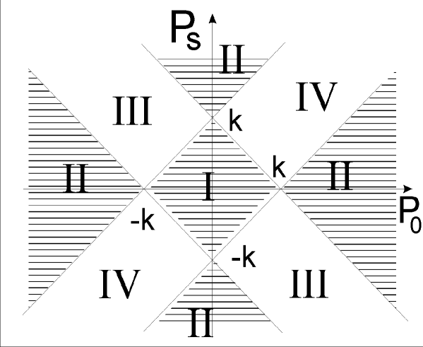
Figure 1: Regions in $p_{0},\ p_{s}$ plane corresponding to bipolar transformations (1-4)

Action of these transformations is shown in Fig.1. After performing these transformations variables in eq.(4) separate:

$$p_{s}\Phi(p_{0},p_{s})=f(\alpha_{i})g(\beta_{i})\ \ \ \ \ \ \ i=1,2,3,4$$

and we obtain the following equations for each of the functions $f$ and $g$:

(a) For transformations $(1)-(2)$ (the shaded regions in Fig.1):

$$\left[\frac{d^{2}}{d\beta^{2}}+h_{1}-\frac{l(l+1)}{\sinh^{2}\beta}\right]g(\beta)=0,$$ (6)

$$\left[\frac{d^{2}}{d\alpha^{2}}+h_{1}-\frac{\lambda/m^{2}}{a-\cosh^{2}\alpha}\right]f(\alpha)=0;$$ (7)

(b) For transformations $(3)-(4)$ (the unshaded regions in Fig.1):

$$\left[\frac{d^{2}}{d\beta^{2}}+h_{2}+\frac{l(l+1)}{\cosh^{2}\beta}\right]g(\beta)=0,$$ (8)

$$\left[\frac{d^{2}}{d\alpha^{2}}+h_{2}-\frac{\lambda/m^{2}}{a+\sinh^{2}\alpha}\right]f(\alpha)=0.$$ (9)

In these equations

$$a\equiv\frac{W^{2}}{m^{2}}>1$$

and $h_{1},h_{2}$ are the separation parameters (new quantum numbers). The fact of separability is provided by the symmetry of relativistic problem in the 4-dimensional world [12].

Equations obtained above describe one-dimensional motions in the space of hyperbolic angles. Equations for $g(\beta)$ are kinematic ones defining the values of separation parameters $h_{1,2}$. Equations for $f(\alpha)$ contain dynamical quantities $(\lambda,a)$ and hence must allow to find the energy spectrum.

Boundary conditions for $g(\beta)$ and $f(\alpha)$ follow immediately from (5) and are the same in different regions of the $(p_{0},p_{s})$-plane

$$g(0)=0 g(\pm\infty)<\infty$$ (10)

$$f(0)<\infty f(\pm\infty)=0$$ (11)

Note that the boundaries of different regions in $(p_{0},p_{s})$-plane can be approached by taking limits $\alpha,\beta\to\pm\infty$ in the relevant transformations $(1)-(4)$.

3 Solutions of the one-dimensional equations

First consider the pair (6)-(7). Eq.(6) with the boundary conditions (10) has the following solution:

$$g(\beta)=g_{l}(\beta)\sim\Biggl{\{}\sinh^{l+1}\beta{\left[\frac{1}{\sinh\beta}\frac{d}{d\beta}\right]^{l+1}\cosh(\sqrt{h_{1}}\beta),\ \ \ \ h_{1}>0}\atop{0,\qquad\qquad h_{1}<0}$$ (12)

In general, the second equation of this pair can give the relation between energy $W$ and the parameter $h_{1}$

$$W=\rho_{n}(h_{1}),\ \ \ \ \ \\ n=0,1,2\ldots$$

Despite the fact that $n$ can take discrete values, energy is not quantized because $h_{1}$ remains to be an artbitrary positive number.

Things are essentially different in the unshaded regions $(3)-(4)$. Eq.(8) has solutions with positive and negative signs of $h_{2}$. The positive $h_{2}$ are not resulted while the negative ones are quanttizes for $l>0$.

$$h_{2}=-(l-N)^{2},\ \ \ \ \ \ N<l.$$

where $N$ takes odd integer values.

Next consider eq.(9) in more detail. Expression

$$V(\alpha)=\frac{\lambda/m^{2}}{a+\sinh^{2}\alpha}$$

plays the role of ”potential”.

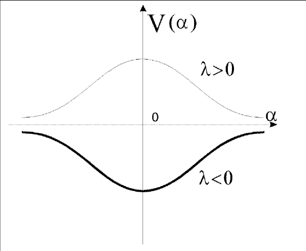
Figure 2: The “potential” $V(\alpha)$ for both signes of $\lambda$.

For positive $\lambda$ (i.e. attraction) $V(\alpha)$ is the positive definite and convex function of $\alpha$ (Fig.2). Obviously we can have only continuous spectrum in this case witth posititve $h_{2}$.

When we take $\lambda$ negative (repulsion) $V(\alpha)$ becomes negative definitte and concave function of $\alpha$ (Fig.2). Therefore in this case there appears principal possibility to have discrete eigenvalues provided the depth of $V(\alpha)$ is high enough for a given negative value of $h_{2}=-(l-N)^{2}$.

One can examine easily that continuity on the boundaries of shaded and unshaded regions imposes no new constraints on separation parameters $h_{1,2}$. So there is no discrete specttrum for positive values of $\lambda$ when $W>m$.

Now we turn back to eqs.(8)-(9) with $h_{2}<0$ and $\lambda<0$. Eq.(8) is a Heun’s differential equation [15]. Its solution with $h_{2}=(l-N)^{2}$ and $\lambda=-|\lambda|<0$ imposed by boundary and normalization conditions leads to complicated transcendential equations. To estimate qualitatively the coupling constant dependence of the energy eigenvalues one can make use of tthe following approximate expression

$$W^{2}\sim\frac{|\lambda|}{\nu(\nu+1)}\ \ \ \ \ \nu=1,2,\ldots$$

As $W^{2}>m^{2}$ it follows that

$$\frac{\lambda^{2}}{m^{2}}\geq\nu(\nu+1)=2,6,12,\ldots$$

i.e. discrete levels apeear when $|\lambda|$ exceeds some critical values. It is worth noting that for some fixed values of $\lambda^{2}/m^{2}$ there is finite number of discrete levels. For example, when

$$2<\frac{\lambda^{2}}{m^{2}}<6$$

there is only a single level. And for

$$6<\frac{\lambda^{2}}{m^{2}}<12$$

the number of levels equals $2$, etc.

If we take $|\lambda|$ in accordance with Balmer formula mentioned above in the following form $\lambda\pi=m^{2}Z^{2}\alpha$, then the above evaluation can be cast into

$$\frac{Z^{2}\alpha}{\pi}>\nu(\nu+1)$$

i.e. $Z_{min}>30$.

We want to note tthat eqs.(8)-(9) were derived earlier in [13] but with erroneous sign of $\lambda$. Hence author deduced bound states for positive values of $\lambda$.

4 Normalization condition

Let us now discuss the normalization condition for the BS amplitude, which is nonvanishing only in the unshaded regions and has the form:

$$\psi(p)\sim\frac{(\sinh\alpha+\sinh\beta)^{3}f(\alpha)g(\beta)}{(W^{2}-m^{2})^{3/2}\cosh^{3}\beta(W^{2}+m^{2}\sinh^{2}\alpha)}Y_{lm}(\theta,\phi)$$ (13)

The role of normalization is to provide the correct relation between the aplitude $\psi$ and four-point Green function. The exact form of the normalization condititon for the model under consideration looks like [1]

$$i\int d^{4}p\bar{\psi}(p)G_{0}^{-1}(p)\psi(p)=\varepsilon_{B}\lambda\frac{dS_{B}(\lambda)}{d\lambda}$$ (14)

where $S_{B}(\lambda)=4W^{2}_{B}(\lambda)$ and $\varepsilon_{B}$ is the so called norm factor determining the sign of the pole contribution in the total Green function at $S\sim S_{B}(\lambda)$

$$G\sim i\varepsilon_{B}\frac{\psi_{B}(p)\bar{\psi}_{B}(p)}{S-S_{B}}+\mbox{Reg}$$ (15)

Integration in the normalization condition (14) is carried over the unshaded region only.

The spectral representation for $\psi(p)$ and $\bar{\psi}(p)$ that we are going to use has the form [1]:

$$\psi(p_{0},\vec{p})=-\frac{1}{2\pi i}\int^{\infty}_{w_{+}(\vec{p})}dq_{0}\frac{f(q_{0},\vec{p},W)}{p_{0}-q_{0}+io}+\frac{1}{2\pi i}\int_{-\infty}^{w_{-}(\vec{p})}dq_{0}\frac{g(q_{0},\vec{p},W)}{p_{0}-q_{0}-io};$$ (16)

$$\bar{\psi}(p_{0},\vec{p})=-\frac{1}{2\pi i}\int^{\infty}_{w_{+}(\vec{p})}dq_{0}\frac{f^{*}(q_{0},\vec{p},W)}{p_{0}-q_{0}+io}+\frac{1}{2\pi i}\int_{-\infty}^{w_{-}(\vec{p})}dq_{0}\frac{g^{*}(q_{0},\vec{p},W)}{p_{0}-q_{0}-io}$$ (17)

where $w_{-}(\vec{p})=W-(\vec{p}^{2}+m^{2})^{1/2},\ \ w_{+}(\vec{p})=-w_{-}(\vec{p})$ are the enndpoints where cuts in the complex $p_{0}$-plane extend from. As long as 3-momentum $\vec{p}$ satisfies $0\leq p_{s}^{2}\leq W^{2}-m^{2}$ these two cuts overlap (Fig.3).

The spectral reprezentations (16)-(17) imply

$$\bar{\psi}(z)=-\psi^{*}(z^{*}),\ \ \ \ \ z=\Re p_{0}+i\Im p_{0}$$ (18)

There are “dangerous” regions in the normalization integral where left-hand and right-hand cuts overlap. This overlapping happens when

$$p_{0}\in{-w_{0},0} \mbox{for right-hand cut},$$

$$p_{0}\in{0,w_{0},0} \mbox{for left-hand cut}.$$

In these intervals $0\leq p_{s}^{2}\leq k^{2}=W^{2}-m^{2}$. In the $(p_{0},p_{s})$-plane “dangerous” points are located between the profiles of functions $w_{+}(\vec{p})$ and $w_{-}(\vec{p})$ for $p_{s}^{2}\leq k^{2}$. This region is drawn in Fig.4.

Note that the “dangerous” points completely lie in the region where our BS amplitude vanishes identically. Therefore, owing to this specific behaviour of the BS amplitude for bound states with $W>m$, intervals of $p_{0}$ where cuts overlap do not contribute to the normalization integral.

It seems to us that this property is very important and can show up in more interesting cases too. Specifically this fact may be employed for confining kernels, because sometimes bound states above threshold ($W>m$) do arise for such kernels. Example considered above indicates that in similar cases the $(p_{0},p_{s})$-plane may bear some structure — namely the BS amplitude may have support region in the $(p_{0},p_{s})$-plane. So effectively we can take that cuts in the spectral representation start from the origin ($p_{0}=0$) and, consequently, perform Wick rotation without any complications. This is the case when Wick rotation is admissible for dynamical reasons. As a result we obtain:

$$i^{2}\int d^{3}pdp_{4}\bar{\psi}(ip_{4},\vec{p})G_{0}^{-1}(ip_{4},\vec{p})\psi(ip_{4},\vec{p})=\varepsilon\lambda\frac{dS_{B}(\lambda)}{d\lambda}$$ (19)

Now, according to (18) and symmetry of eq.(3) under the relative time reflection $p_{0}\to-p_{0}$ we have:

$$\bar{\psi}(ip_{4},\vec{p})=\psi^{*}(-ip_{4},\vec{p})=-\Pi_{B}\psi^{*}(ip_{4},\vec{p}),$$ (20)

where $\Pi_{B}$ denotes the so-called relative-time parity (“$p_{0}$-parity”) of the bound state.

Using (20) in the normalization integral we get

$$\int d^{3}pdp_{4}\bar{\psi}(ip_{4},\vec{p})G_{0}^{-1}(ip_{4},\vec{p})\psi(ip_{4},\vec{p})=\varepsilon\lambda\frac{dS_{B}(\lambda)}{d\lambda}$$

As long as $G_{0}^{-1}(ip_{4},\vec{p})$ is positive definite in the unshaded regions the full integral above is positive definite too. Besides, from the explicit form of our solution we know that

$$\lambda\frac{dS_{B}(\lambda)}{d\lambda}=|\lambda|\frac{dS_{B}(\lambda)}{d|\lambda|}>0$$

and therefore with appropriate choice of overall multiplicative constant up to which the BS amplitude is determined the norm factor $\varepsilon_{B}$ coinsides with “$p_{0}$-parity” of the bound state

$$\varepsilon_{B}=\Pi_{B}\ .$$

In other words the states with positive (negative) “$p_{0}$-parity” have the positive (negative) norm.

States with the negative norm can be be eliminated in from the physical sector as the correspondinng “one-time” quasipotential wave functions [16] vanish identically:

$$\int^{\infty}_{-\infty}dp_{0}\psi(p_{0},\vec{p})=0\ .$$

On the other hand the positive norm states, i.e. the states with positive “$p_{0}$-parity” do survive and produce the pole contributions to the total Green function (and S-matrix) with the correct sign.

5 Conclusions

We have demonstrated that in the BS equation for the equal mass scalar particles’ repulsive ($\lambda<0$) interaction via scalar massless particle exchange there emerges an effective attraction above thershold. This attraction can lead to existence of bound states for values of the coupling $\lambda$ larger then the critical one:

$$\frac{|\lambda_{c}|}{m^{2}}>2\ .$$

In QED with the one-photon exchange this corresponds to

$$\frac{\alpha_{c}}{\pi}>2\ .$$

It is worth mentioning that attraction is present for all values of $\lambda$ as a purely relativistic effect in the kinematic region where the retardation effects can not be treated by perturbative methods.

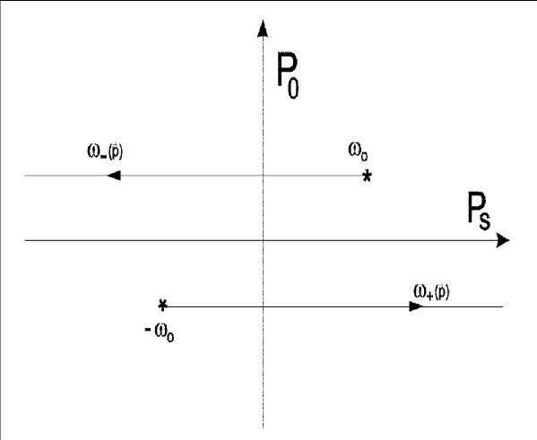
Figure 3: Complex $p_{0}$ plane. Here $\omega_{0}=[\omega_{-}(\vec{p})_{max}=W-m>0$.

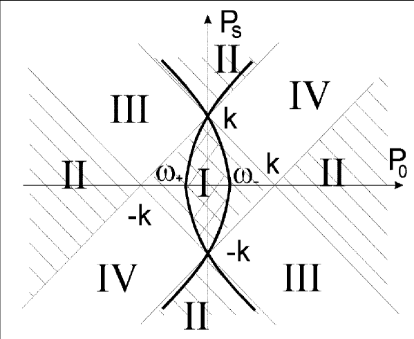
Figure 4: “Dangerous” region in the $p_{0},\ p_{s}$ plane.

References

- [1] N. Nakanishi. Suppl. of Progr. Theor. Phys. 43, (1969) 1.
- [2] A. A. Khelashvili, A. N. Tavkhelidze, L. G. Vachnadze.“Discrete eigenvalues with positive energies in Qauntum Field Theory”. Preprint TMI P-07, Tbilisi, 1991.
- [3] T. Cowan et al. Phys. Rev. Lett. 56, (1986) 444.
- [4] B. Arbuzov et al. TMF 83, (1990) 175.
- [5] J. Spence, J. Vary. Phys. Lett.B254, (1991) 1.
- [6] G. C. Wick. Phys. Rev. 96, (19554) 1124.
- [7] M. Günter. Phys. Rev. D9, (1974) 2411.
- [8] R. Kusaka, A. G. Williams. Preprint ADP-95-28/T182; hep-ph/9505208.
- [9] M. Harada, Y. Yoshida. Preprint KUNS-1304; SU-4240-592; hep-ph/9505206.
- [10] R. E. Cutkosky. Phys. Rev. 96, (1954) 1135.
- [11] H. S. Green. Nuovo Cim. 5, (1957) 866.
- [12] V. A. Fock. Zs. Physik, 98, (1958) 145.
- [13] S. N. Biswas. Nuovo Cim. 7 (1958) 577.
- [14] H. S. Green, S. N. Biswas. Phys. Rev. 171, (1968) 1511.
- [15] G. Bateman, A. Erdelyi. High Transcendental Functions, v.2 (1968).
- [16] A. A. Logunov, A. N. Tavkhelidze. Nuovo Cim. 29, (1963) 380.