BROWN-HET-1233

CU-TP-981

IAS-SNS-99/114

PUPT-1942

hep-th/0007051

Black Hole Thermodynamics from Calculations in Strongly-Coupled Gauge Theory

Daniel Kabat^1,2, Gilad Lifschytz^3,4 and David A. Lowe⁵

¹Department of Physics

Columbia University, New York, NY 10027

kabat@physics.columbia.edu

²School of Natural Sciences

Institute for Advanced Study, Princeton, NJ 08540

³Department of Physics

Princeton University, Princeton, NJ 08544

gilad@viper.princeton.edu

⁵Department of Physics

Brown University, Providence, RI 02912

lowe@het.brown.edu

We develop an approximation scheme for the quantum mechanics of $N$ D0-branes at finite temperature in the ’t Hooft large-$N$ limit. The entropy of the quantum mechanics calculated using this approximation agrees well with the Bekenstein-Hawking entropy of a ten-dimensional non-extremal black hole with 0-brane charge. This result is in accord with the duality conjectured by Itzhaki, Maldacena, Sonnenschein and Yankielowicz. Our approximation scheme provides a model for the density matrix which describes a black hole in the strongly-coupled quantum mechanics.

1 Introduction

Properties of black holes in quantum theories of gravity have intrigued physicists for many years. In recent years much progress has been made in understanding some of these properties using string theory. However because string theory is usually formulated perturbatively about a given spacetime background, it has been difficult to obtained a unified and complete description of black hole physics. In the past few years nonperturbative formulations of string theory have been proposed in terms of large $N$ gauge theories. These formulations give new hope for understanding some of these fundamental issues.

In particular, Maldacena’s conjecture gives a promising arena to answer some of these questions. Maldacena’s conjecture [1] relates string theories in anti-de Sitter backgrounds to conformal field theories in a large-$N$ limit. However there is no free lunch. In this framework, seemingly obvious questions on the string theory side are hard to formulate on the gauge theory side. Moreover, in the range of parameters where semi-classical string theory may be used to construct black hole geometries, the dual gauge theory is strongly coupled. This makes understanding black hole states very difficult.

One way of dealing with these difficulties is to perform Monte Carlo simulations of the gauge theory at strong coupling [2, 3]. In the present work we pursue a different approach, in which we begin with an ansatz for the density matrix which describes the black hole in the continuum gauge theory.

The version of Maldacena duality to be considered here relates black holes in ten dimensions with 0-brane charge to supersymmetric gauged $SU(N)$ quantum mechanics with sixteen supercharges [4]. The metric of the non-extremal black hole is

$$ds^{2} = \alpha^{\prime}\left[-h(U)dt^{2}+h^{-1}(U)dU^{2}+{c^{1/2}(g_{YM}^{2}N)^{1/2}\over U^{3/2}}d\Omega_{8}^{2}\right]$$

$$h(U) = \frac{U^{7/2}}{c^{1/2}(g_{YM}^{2}N)^{1/2}}\left(1-\frac{U_{0}^{7}}{U^{7}}\right)$$ (1)

where $c=2^{7}\pi^{9/2}\Gamma(7/2)$ and $g_{YM}$ is the Yang-Mills coupling constant. The horizon of the black hole is at $U=U_{0}$, which corresponds to a Hawking temperature

$$T=(g^{2}_{YM}N)^{-1/2}\left(U_{0}\over 11.1\right)^{5/2}\,.$$ (2)

The dual quantum mechanics is to be taken at the same finite temperature. The black hole has a free energy, which arises from its Bekenstein-Hawking entropy [5].

$$\beta F=-2.52~{}N^{2}\left({T\over(g_{YM}^{2}N)^{1/3}}\right)^{1.80}$$ (3)

Duality predicts that the quantum mechanics should have the same free energy. The supergravity description is expected to be valid when the curvature and the dilaton are small near the black hole horizon. This regime corresponds to the ’t Hooft large $N$ limit of the quantum mechanics, when the dimensionless effective coupling $g_{YM}^{2}N/T^{3}$ is large.

In this report we describe a set of approximations that can be applied to the quantum mechanics in the regime of interest. Using these techniques we calculate the finite temperature partition function of the quantum mechanics. Over a certain range of temperature our results can be well fit by a power law,

$$\beta F\approx{\rm const.}-2.0~{}N^{2}\left({T\over(g^{2}_{YM}N)^{1/3}}\right)^{1.7}\,.$$ (4)

This is in quite good agreement with the black hole prediction (3). We believe this is the first nontrivial direct test of a strong/weak coupling duality that does not rely on supersymmetric non-renormalization theorems or special properties of BPS states. Although in the present paper we are primarily interested in the thermodynamics of the quantum mechanics, our approximation scheme should also be useful for addressing questions about the spacetime structure of the black hole, perhaps along the lines of [6, 7].

The basic idea is to treat the ${\cal O}(N^{2})$ degrees of freedom of the quantum mechanics as statistically independent, using a type of mean field approximation. This assumption is motivated by the overall $N^{2}$ dependence of the free energy (3). The approximation involves constructing a trial action $S_{0}$ from the full action $S$. All quantities can then be systematically computed as an expansion in powers of $S-S_{0}$. The parameters in the trial action are fixed by solving a truncated version of the Schwinger-Dyson equations of the quantum mechanics. This procedure can be viewed as re-summing an infinite number of Feynman diagrams. Since we are interested in large-$N$ behavior, we will only resum planar diagrams. Thus, in our approximation, the overall $N^{2}$ factor in the free energy (4) and the appearance of $g_{YM}^{2}$ only in the combination $g_{YM}^{2}N$ is guaranteed. The crucial test of the approximation is to obtain the correct dependence of the thermodynamics on the effective dimensionless coupling $g_{\rm eff}^{2}=g_{YM}^{2}N/T^{3}$.

The sort of approximation that we are considering has several attractive features, which we regard as a priori reasons to believe that it captures some of the essential physics of the strongly-coupled quantum mechanics.

• As mentioned above, the approximation automatically respects ’t Hooft large-$N$ counting.

• The approximation partially respects the symmetries of the problem. More precisely, it respects all symmetries which act linearly on the fields. Thus our trial action will have ${\cal N}=2$ supersymmetry and $SO(2)\times SO(7)$ rotational symmetry (out of the underlying ${\cal N}=16$ supersymmetry and $SO(9)$ rotational symmetry).

• The approximation is non-perturbative in the Yang-Mills coupling constant, and self-consistently cures the infrared divergences present in conventional perturbation theory.

Before continuing there is one other issue we would like to comment on. The partition function of the full quantum mechanics contains an infrared divergence from the regions in moduli space when the D0-branes are far apart. This leads to a divergent contribution to the entropy with an overall coefficient ${\cal O}(N)$. From the supergravity point of view, this corresponds to a thermal gas of gravitons. This divergence may be regulated by putting the system in a finite box. The black hole entropy which is ${\cal O}(N^{2})$ can easily be made to dominate over the ${\cal O}(N)$ contribution. Our mean field approximation computes the ${\cal O}(N^{2})$ piece by design, and this infrared divergence does not make an appearance.

2 Gaussian Approximation for 0-brane Quantum Mechanics

In this section we sketch the application of the Gaussian approximation [8] to gauged $SU(N)$ supersymmetric quantum mechanic with sixteen supercharges. Further details will appear in [9].

One key requirement is that supersymmetry, although softly broken by the finite temperature of the black hole, should not be broken explicitly by the approximation. To avoid such explicit breaking we adopt an unconstrained superfield formulation, in which supersymmetry acts linearly on the fields. This ensures that we recover exact supersymmetry in the zero temperature limit. We will use an ${\cal N}=2$ superspace so that only an $SO(2)\times G_{2}$ subgroup of the $SO(9)$ R-symmetry is manifest. First let us recall the superspace and supermultiplets that we are going to use; for more details on notation see [8].

With ${\cal N}=2$ supersymmetry we have an $SO(2)$ R-symmetry, with spinor indices $\alpha,\beta=1,2$ and vector indices $i,j=1,2$. The $SO(2)_{R}$ Dirac matrices $\gamma^{i}_{\alpha\beta}$ are real, symmetric, and traceless. Given two spinors $\psi_{\alpha}$ and $\chi_{\alpha}$, besides the invariant $\psi_{\alpha}\chi_{\alpha}$, one can construct a second invariant which we denote

$$\psi^{\alpha}\chi_{\alpha}={i\over 2}\epsilon_{\alpha\beta}\psi_{\alpha}\chi_{\beta}\,.$$

${\cal N}=2$ superspace has coordinates $(t,\theta_{\alpha})$ where $\theta_{\alpha}$ is real. We denote $\theta^{2}=\theta^{\alpha}\theta_{\alpha}$, and define the supercovariant derivative

$$D_{\alpha}={\partial\over\partial\theta_{\alpha}}-i\theta_{\alpha}{\partial\over\partial t}~{}.$$ (5)

The simplest representation of supersymmetry is a real scalar superfield

$$\Phi=\phi+i\psi_{\alpha}\theta_{\alpha}+f\theta^{2}$$ (6)

containing a scalar field $\phi$, its superpartner $\psi_{\alpha}$, and an auxiliary field $f$. The gauge superfield denoted by $\Gamma_{\alpha}$ has an expansion in ‘linear’ components as

$$\Gamma_{\alpha}=\chi_{\alpha}+A_{0}\theta_{\alpha}+X^{i}\gamma^{i}_{\alpha\beta}\theta_{\beta}+d\epsilon_{\alpha\beta}\theta_{\beta}+2\epsilon_{\alpha\beta}\lambda_{\beta}\theta^{2}\,.$$ (7)

The fields $X^{i}$ are physical scalars, while $\lambda_{\alpha}$ are their superpartners, $d$ is an auxiliary boson, $\chi_{\alpha}$ are auxiliary fermions, and $A_{0}$ is the 0+1 dimensional gauge field.

To construct our action we introduce a collection of seven adjoint scalar multiplets $\Phi_{a}$ transforming in the ${\bf 7}$ of $G_{2}\subset SO(9)$. The ${\cal N}=16$ supersymmetric $SU(N)$ gauged quantum mechanics action is

$$S_{\rm sym}={1\over g^{2}_{\rm YM}}\int dtd^{2}\theta\,{\rm Tr}\left(-{1\over 4}\nabla^{\alpha}{\cal F}_{i}\nabla_{\alpha}{\cal F}_{i}-\frac{1}{2}\nabla^{\alpha}\Phi_{a}\nabla_{\alpha}\Phi_{a}-\frac{i}{3}f_{abc}\Phi_{a}[\Phi_{b},\Phi_{c}]\right)$$

where ${\cal F}_{i}$ is the field strength constructed from the gauge multiplet, $\nabla_{\alpha}=D_{\alpha}+\Gamma_{\alpha}$, and $f_{abc}$ is a suitably normalized totally antisymmetric $G_{2}$-invariant tensor.

We impose the supersymmetric gauge condition $D^{\alpha}\Gamma_{\alpha}=0$, which sets $\partial A_{0}/\partial t=0$, $d=0$ and $\lambda=\frac{1}{2}\partial\chi/\partial t$. This is a convenient gauge fixing, as this gauge condition helps make the approximation compatible with Ward identities [9]. To the SYM action we must add the corresponding ghost action (but no gauge fixing term)

$$S_{\rm ghost}={1\over g^{2}_{\rm YM}}\int dtd^{2}\theta\,{\rm Tr}\left(D^{\alpha}\bar{C}\nabla_{\alpha}C\right)$$

where the ghost superfield $C$ is a complex scalar superfield with Grassmann statistics.

We are interested in the finite temperature behavior of the quantum mechanics. As usual we compactify the Euclidean time coordinate on a circle of circumference $\beta$, which is identified with the inverse temperature. The bosonic fields have integer mode expansions, while the fermions have half integer modes; for example we write

$$X^{i}(\tau)={1\over\sqrt{\beta}}\sum_{l\in{\mathbb{Z}}}X_{l}^{i}e^{i2\pi l\tau/\beta}\,.$$

Note that in Euclidean space the zero mode of the gauge field, which we denote $A_{00}$, survives as a physical degree of freedom (fluctuations in $A_{0}$ are eliminated by our gauge condition).

Our strategy is to construct a trial action $S_{0}$, which we use as an approximation to the full action $S=S_{\rm sym}+S_{\rm ghost}$. The free energy can then be calculated as an expansion in powers of $S-S_{0}$; note that such an expansion is non-perturbative in the original Yang-Mills coupling $g^{2}_{YM}$. Throughout this paper we use the following expression for the free energy in this scheme.

$$\beta F\approx\beta F_{0}+\langle S-S_{0}\rangle_{0}-\frac{1}{2}\langle S_{III}^{2}\rangle_{{\hbox{\cmsss C}},0}$$ (8)

Here $\beta F_{0}$ is the free energy of the trial action, and $\langle\cdot\rangle_{0}$ denotes an expectation value computed using $S_{0}$. Also $S_{III}$ refers to cubic terms in the original SYM plus ghost action, and the subscript C denotes a connected correlation function. It is straightforward, though tedious, to compute higher order terms in the expansion of $\beta F$. In principle this could be used as a check on the validity of the approximation.

We make the following ansatz for the trial action:

$$S_{0}=-\frac{N}{\lambda}{\rm Tr}(U+U^{\dagger})+\sum_{l,i}\frac{1}{2\sigma_{l}^{2}}{\rm Tr}(X^{i}_{l}X^{i}_{-l})+\sum_{l,a}\frac{1}{2\Delta_{l}^{2}}{\rm Tr}(\phi^{a}_{l}\phi^{a}_{-l})+\cdots\,.$$ (9)

Here all fields (except the gauge field) appear in Gaussian form. Indeed this is the most general Gaussian action which is quadratic in the fundamental fields. This means that the trial action can respect all symmetries which act linearly on the fundamental fields.

The gauge field must be treated in a special way, owing to its periodicity properties. To do this we have introduced the timelike Wilson loop operator $U$, which can be expressed in terms of the gauge zero mode.

$$U=Pe^{i\int_{0}^{\beta}A_{0}}=e^{i\sqrt{\beta}A_{00}}$$

This makes it manifest that at finite temperature $A_{0}\sim A_{0}+2\pi/\beta$ is periodic. As a trial action for the gauge field we have adopted the unitary one plaquette model action. As $\lambda$ varies the trial action goes through a Gross-Witten phase transition at $\lambda=2$ [10].

The key step in the approximation is to find a closed set of “gap” equations for the dressed propagators $\sigma_{l}^{2},\,\Delta_{l}^{2},\,\ldots$ appearing in (9). Again, the gauge field must be treated as a special case. All other propagators are obtained by demanding stationarity of the estimate (8) for the free energy. Up to contributions from the gauge field, it can be shown this procedure correctly re-sums all one-loop self-energy corrections to the propagators.

The gap equation for $\lambda$ is obtained from the Schwinger-Dyson equation for $\langle U\rangle$ that arises from the change of variables $U\to gU$ with $g\in SU(N)$. Demanding that this equation hold with respect to the one-plaquette measure yields

$$\langle{\rm Tr}U\rangle_{0}=\frac{1}{\beta^{3/2}}{\rm Tr}\left\langle U\left(\frac{\delta S}{\delta A_{00}}-\frac{1}{2}\frac{\delta S_{III}^{2}}{\delta A_{00}}\right)\right\rangle_{C,0}~{}.$$ (10)

This equation resums one-loop corrections to the Wilson loop, in the same sense that stationarizing (8) resums one-loop corrections to the propagators. At large $N$ the terms on the right hand side factorize into a gauge field correlator times matter field correlators; the terms involving the gauge fields may be computed using the results of [10].

As (8), (10) are somewhat lengthy expressions we will not present them here. Rather we report on the solution to these equations in the next section.

3 Numerical Results

The gap equations can be solved numerically, using the methods discussed in Appendix B of [8]. The basic strategy is to start at high temperature, where the gap equations can be solved semi-analytically, then use Newton-Raphson to solve the gap equations at a sequence of successively lower temperatures. As mentioned in the introduction, $g_{YM}^{2}$ and $N$ only appear in the combination $g_{YM}^{2}N/T^{3}$. Henceforth we choose units for $T$ which effectively scales $g_{YM}^{2}N$ to $1$.

In principle the resulting Gaussian action contains a great deal of information about correlation functions in the quantum mechanics. But in this section we will just concentrate on the behavior of three basic quantities: the free energy, the Wilson loop, and the mean size of the state.

At high temperature, where the gauge theory is weakly coupled, we find that the free energy of the system is

$$\beta F=6\log\beta+{\cal O}(1)\,.$$ (11)

This result can be obtained analytically: the gap equations are dominated by the bosonic zero modes, and the free energy is dominated by $\beta F_{0}$.

In general, for a weakly-coupled theory in $0+1$ dimensions, one would expect the free energy to behave like $\log\beta$. But note that, even though the gauge theory is weakly coupled at high temperature, the perturbation series is afflicted with IR divergences. Thus, to determine the coefficient of the logarithm (which depends on the value of the dynamically generated IR cutoff) one must re-sum part of the perturbation series. This is a well-known phenomenon in finite temperature field theory [12]. In any case, we expect a priori that the Gaussian approximation gives good results in the high temperature regime.

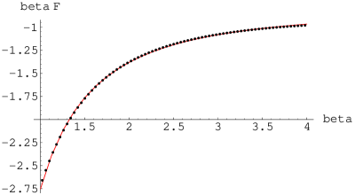
Figure 1: The solid curve is the power law fit (12) for $\beta F$. The data points are calculated from numerical solutions to the gap equations.

As the temperature is lowered the behavior of the free energy changes: at $\beta\approx 0.7$ we find that it begins to roll over and fall off as a non-trivial power of the temperature. In the range $1<\beta<4$ the numerical results for the free energy are well fit by

$$\beta F\approx-0.79-2.0~{}\beta^{-1.7}\,.$$ (12)

This fit to the numerical results is illustrated in Fig. 1. Note that supersymmetry is crucial in making such power-law behavior possible. Without supersymmetry the free energy would behave as $\beta F\approx\beta E_{0}$ in the low temperature regime $\beta>1$, where $E_{0}$ is the ground state energy of the system.

We obtained (12) by performing a Levenberg-Marquardt nonlinear least-squares fit to 75 numerical calculations of the free energy, carried out in the temperature range $1\leq\beta\leq 4$. To estimate the uncertainty in the best fit parameters we varied the window of $\beta$ over which the fit was performed (fitting over the ranges $2<\beta<4$ and $1<\beta<3$), which leads to: $-0.79\pm 0.06$, $-2.0\pm 0.1$ and $-1.7\pm 0.2$.

It is quite remarkable that the power law (12) is in excellent agreement with the semiclassical black hole prediction [4]

$$\beta F=-2.52~{}\beta^{-1.80}\,.$$ (13)

The exponents differ by 6% while the coefficients of the power-law differ by 26%. (An additive constant appears in the Gaussian approximation for the free energy. We will generally ignore this ‘ground state degeneracy’, since it seems to be an artifact of the Gaussian approximation when applied to systems with a continuous spectrum. Similar behavior was noted in [8].)

As we go to still lower temperatures, we find that the energy $\partial(\beta F)/\partial\beta$ calculated in the Gaussian approximation begins to drop below the energy of the black hole. In fact the Gaussian energy becomes negative around $\beta=5.8$. Ultimately, as $\beta\rightarrow\infty$, the Gaussian energy does asymptote to zero, as required by the ${\cal N}=2$ supersymmetry which is manifest in the approximation. But a negative energy clearly reflects some problem with the approximation.

Fortunately, we can be rather precise about exactly where the approximation is going wrong: the difficulty is with the Schwinger-Dyson gap equation we have been using to fix the value of the one-plaquette coupling $\lambda$. Although we do not know how to write down a better gap equation for $\lambda$, we can give a prescription for fixing $\lambda$, that will allow us to obtain reasonable results at much lower values of the temperature. This may be regarded either as a check on our understanding of why the approximation is breaking down, or as a way of building a model for the black hole that can be used at lower temperatures. Our prescription for fixing $\lambda$ is simply that, when $\beta>2.5$ (the midpoint of our range $1\leq\beta\leq 4$), we choose $\lambda$ so that the free energy is given by (12).

Figure 2: Energy vs. $\beta$. For $\beta>2.5$ fixing $\lambda$ by fitting $\beta F$ to a power law leads to the solid middle line, while the Schwinger-Dyson gap equation for lambda leads to the lower dashed line. The upper dot-dashed line is the semiclassical energy of the black hole.

Figure 3: Energy vs. $\beta$. Same as Fig. 2, but plotted on a $\log$–$\log$ scale.

Figure 4: The one-plaquette coupling $\lambda$ vs. $\beta$. The Gross-Witten transition occurs when $\lambda=2$. For $\beta<2.5$ we use the Schwinger-Dyson gap equation to determine $\lambda$. For $\beta>2.5$ the Schwinger-Dyson gap equation gives the dashed line, while fitting $\beta F$ to a power law gives the solid line.

The energy $E=\partial(\beta F)/\partial\beta$ calculated with this prescription is shown in Figs. 2 and 3. The behavior of $\lambda$ given by this prescription is shown in Fig. 4. Note that $\lambda$ increases monotonically with $\beta$. A Gross-Witten phase transition takes place when $\lambda=2$; this value is reached at $\beta=7.8$. Thus a phase transition takes place as the system moves into the supergravity regime [8].

By adopting the prescription of fitting $\beta F$ to a power law, we cannot say anything about the order of the phase transition. If one takes the Schwinger-Dyson result for $\lambda$ seriously, then the Gross-Witten transition occurs at $\beta=14.2$, and is second order (the second derivative of the free energy drops by $0.01$ in crossing the transition).

Our prescription for choosing $\lambda$ begins to break down around $\beta=14$, as we find that $\lambda$ rapidly diverges as $\beta$ approaches 14. By itself, this is not necessarily a problem: infinite $\lambda$ simply means that the Wilson loop is uniformly distributed over $U(N)$. But unfortunately, we do not have a good prescription for continuing past this temperature. Evidently some of the other gap equations (not just the gap equation for $\lambda$) start to break down at this point. Note that this breakdown does not occur until well into the strong coupling regime, as an inverse temperature $\beta=14$ corresponds to an effective gauge coupling $g_{\rm eff}^{2}=\beta^{3}\approx 3\times 10^{3}$.

Finally, let us comment on the average ‘size’ of the state. In our approximation the scalar fields $X^{i}(\tau)$ and $\phi^{a}(\tau)$ are Gaussian random matrices, and their eigenvalues obey a Wigner semi-circle distribution. We can define the size of the state in terms of the quantities

$$R^{2}_{\rm scalar} = {1\over N}{\rm Tr}\langle\left(X^{i}(\tau)\right)^{2}\rangle_{0}~{},$$

$$R^{2}_{\rm gauge} = {1\over N}{\rm Tr}\langle\left(\phi^{a}(\tau)\right)^{2}\rangle_{0}\,.$$ (14)

The radius of the Wigner semi-circle, given by $2\sqrt{R^{2}}$, is shown in Fig. 5. Note that the radius stays fairly constant in the region corresponding to the black hole. However, because the superfield formalism we are using does not respect the full $SO(9)$ invariance, the radius measured in the scalar multiplet directions is not the same as the radius measured in the gauge multiplet directions. At $\beta=14$ we find

$$2R_{\rm scalar}=1.81\qquad\quad 2R_{\rm gauge}=0.80\,.$$

This shows that, as expected, the trial action does not respect the underlying $SO(9)$ invariance. Nonetheless, the trial action may provide a useful approximate description of the black hole density matrix in the supergravity regime.

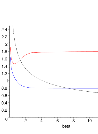
Figure 5: Range of eigenvalues (radius of the Wigner semi-circle) vs. $\beta$. The upper solid red curve is for the scalar fields in the scalar multiplets; the lower solid blue curve is for the scalar fields in the gauge multiplet. The dashed black curve is the Schwarzschild radius of the black hole. These results were calculated with $\beta F$ fit to a power law for $\beta>2.5$.

In Fig. 5 we have also plotted the Schwarzschild radius of the black hole $U_{0}/2\pi=1.76~{}\beta^{-2/5}$. Note that, as the temperature decreases, the Schwarzschild radius becomes much smaller than the radius of the eigenvalue distributions. It seems appropriate to identify the radius of the eigenvalue distributions with the size of the region $U\ll(g^{2}_{\rm YM}N)^{1/3}$ in which 10-dimensional supergravity is valid [4]. The Gaussian approximation should provide a good laboratory for studying the way in which the horizon of the black hole can be detected in the dual quantum mechanics, perhaps along the lines suggested in [6, 7].

4 Discussion

To summarize, we have presented an ansatz for a trial action which captures some of the behavior of 0-brane quantum mechanics at large $N$ and strong coupling. The parameters appearing in the trial action are chosen according to a set of gap equations which resum an infinite set of planar diagrams. The approximation automatically respects ’t Hooft large-$N$ counting, and also partially respects the supersymmetries and R-symmetries of the quantum mechanics.

Our main result is that we obtained a non-trivial power law for the free energy, which is in remarkably good agreement with the black hole prediction. The power law was obtained by fitting numerical results calculated in the range $1<\beta<4$; we would like to emphasize that in this range of temperature the approximation involves no arbitrary or adjustable parameters. We also gave a prescription for fixing the expectation value of the Wilson loop, which allowed us to extend our results to $\beta=14$. This is well into the strong coupling regime, where the supergravity description of the system should be valid.

Although our prescription for fixing the Wilson loop cannot be regarded as entirely satisfactory, it does let us build a model for the black hole density matrix in the strongly-coupled quantum mechanics. This model could be a basis for further studies of black hole properties. It would be particularly interesting to address questions of spacetime locality and causality from the gauge theory point of view, perhaps along the lines suggested in [6, 7].

Acknowledgments

DK wishes to thank Rutgers University and New York University for hospitality, and Emil Martinec and Mark Stern for valuable discussions. The work of DK is supported by the DOE under contract DE-FG02-90ER40542 and by the generosity of Martin and Helen Chooljian. GL would like to thank the Aspen Center for Physics for hospitality, and Vipul Periwal for useful discussions. The work of GL is supported by the NSF under grant PHY-98-02484. D.L. wishes to thank the Aspen Center for Physics, the Abdus Salam International Centre for Theoretical Physics and the Erwin Schroedinger Institute program in Duality, String Theory and M-Theory for hospitality during the course of this research. The research of D.L. is supported in part by DOE grant DE-FE0291ER40688-Task A.

References

- [1] J. Maldacena, The large limit of superconformal field theories and supergravity, Adv. Theor. Math. Phys. 2 (1998) 231, hep-th/9711200.
- [2] R. A. Janik and J. Wosiek, Towards the matrix model of M-theory on a lattice, hep-th/0003121.
- [3] J. Ambjorn, K. N. Anagnostopoulos, W. Bietenholz, T. Hotta and J. Nishimura, Monte Carlo studies of the IIB matrix model at large , hep-th/0005147.
- [4] N. Itzhaki, J.M. Maldacena, J. Sonnenschein and S. Yankielowicz, Supergravity and the large limit of theories with sixteen supercharges, Phys. Rev. D58 (1998) 046004, hep-th/9802042.
- [5] I. R. Klebanov and A. A. Tseytlin, Entropy of Near-Extremal Black -branes, hep-th/9604089.
- [6] D. Kabat and G. Lifschytz, Tachyons and black hole horizons in gauge theory, JHEP 9812 (1998) 002, hep-th/9806214.
- [7] D. Kabat and G. Lifschytz, Gauge theory origins of supergravity causal structure, hep-th/9902073.
- [8] D. Kabat and G. Lifschytz, Approximations for strongly-coupled supersymmetric quantum mechanics, Nucl. Phys. B571 (2000) 419, hep-th/9910001.
- [9] D. Kabat, G. Lifschytz and D.A. Lowe, to appear.
- [10] D. Gross and E. Witten, Possible third-order phase transition in the large- lattice gauge theory, Phys. Rev. D21 (1980) 446.
- [11] J. Cornwall, R. Jackiw and E. Tomboulis, Effective action for composite operators, Phys. Rev. D10 (1974) 2428.
- [12] L. Dolan and R. Jackiw, Symmetry behavior at finite temperature, Phys. Rev. D9 (1974) 3320.