226E 226F

CENTRE DE PHYSIQUE THÉORIQUE

CNRS - Luminy, Case 907

13288 Marseille Cedex 9

SPIN GROUP AND ALMOST COMMUTATIVE GEOMETRY

Thomas SCHÜCKER

Abstract

For Connes’ spectral triples, the group of automorphisms lifted to the Hilbert space is defined and used to fluctuate the metric. A few commutative examples are presented including Chamseddine and Connes’ spectral unification of gravity and electromagnetism. One almost commutative example is treated: the full standard model. Here the lifted automorphisms explain O’Raifeartaigh’s reduction $SU(2)\times U(3)/{\mathbb{Z}}_{2}.$

PACS-92: 11.15 Gauge field theories
MSC-91: 81T13 Yang-Mills and other gauge theories

july 2000
CPT-00/P.4031
hep-th/yymmxxx

1 Introduction

The standard model of electro-weak and strong forces remains the most painful humiliation of theoretical physics. It is hard to believe that its theoretical input,

• the compact, real Lie group $G=SU(2)\times U(1)\times SU(3)/({\mathbb{Z}}_{2}\times{\mathbb{Z}}_{3})$ for the gauge bosons,

• the three unitary representations ${\cal H}_{L},\ {\cal H}_{R},\ {\cal H}_{S}$ for left- and right-handed spinors and the Higgs scalars,

  $${\cal H}_{L} = \bigoplus_{1}^{3}\left[(2,{\textstyle\frac{1}{6}},3)\oplus(2,-{\textstyle\frac{1}{2}},1)\right],$$ (1)

  $${\cal H}_{R} = \bigoplus_{1}^{3}\left[(1,{\textstyle\frac{2}{3}},3)\oplus(1,-{\textstyle\frac{1}{3}},3)\oplus(1,-1,1)\right],$$ (2)

  $${\cal H}_{S} = (2,-{\textstyle\frac{1}{2}},1),$$ (3)

  where $(n_{2},y,n_{3})$ denotes the tensor product of an $n_{2}$ dimensional representation of $SU(2)$, the one dimensional representation of $U(1)$ with hypercharge $y$: $\rho(\exp(i\theta))=\exp(iy\theta)$ and an $n_{3}$ dimensional representation of $SU(3)$. For historical reasons the hypercharge is an integer multiple of ${\textstyle\frac{1}{6}}$.

• 18 real constants: 3 gauge couplings $g_{2},g_{1},g_{3}$, 2 scalar couplings $\lambda,\mu$, 13 Yukawa couplings parameterizing the fermions mass matrix,

and its complicated rules deriving from five action terms:

• the Yang-Mills action,

• the Dirac action,

• the Klein-Gordon action,

• the Higgs potential,

• the Yukawa terms,

encode a fundamental theory. Since several decades experiments continue to confirm the standard model with ever increasing accuracy. Simultaneously all theoretical attempts to lessen the humiliation, technicolour, left-right symmetric models, grand unification, supersymmetry, supergravity, superstrings,… have only added to the humiliation, all attempts except one: Connes’. Like Minkowskian geometry induces the magnetic force from the electric force, Connes’ noncommutative geometry [1] induces some very special Yang-Mills and Higgs forces from the gravitational force via particular generalized coordinate transformations [2][3][4]. At the same time, when acting on both the Dirac and Yang-Mills actions, these coordinate transformations generate the Yukawa terms, the Klein-Gordon action and the Higgs potential with its spontaneous symmetry breaking.

The standard model is in this very special class of Yang-Mills-Higgs models as long as it fulfils the following requirements:

• Only weak isospin doublets and singlets, only colour triplets and singlets occur in the fermion representations.

• At least one neutrino is massless.

• The gauge symmetry of the gauge bosons that violate parity is spontaneously broken by one complex Higgs doublet. The corresponding weak gauge bosons, $W^{\pm},\ Z$ are massive and $\rho:=m_{W}^{2}/(\cos^{2}\theta_{w}\,m_{Z}^{2})=1.$

• There is a Yang-Mills force, whose gauge group commutes with weak isospin, hypercharge and with the fermionic mass matrix, whose gauge group is unbroken and whose couplings to fermions are vectorial. Its gauge bosons, the gluons, are massless [5].

• The hypercharges are such that one of O’Raifeartaigh’s reduction [6], namely to $SU(2)\times U(1)\times SU(3)/{\mathbb{Z}}_{3}$ is possible. This requirement permits the introduction of the unimodularity condition [7], the only ad hoc feature in Connes’ formulation.

• The coupling constants are constrained by $g_{2}^{2}=g_{3}^{2}={\textstyle\frac{5}{3}}g_{1}^{2}=3\lambda.$

All these properties of the standard model are vital for its geometrical interpretation: any version of the standard model not satisfying one of these requirements cannot be derived from gravity à la Connes.

We interpret the relations among the coupling constants to hold at some energy scale $\Lambda$. At this energy scale, the noncommutativity of spacetime starts to be felt. Below this scale, spacetime can be treated as a manifold. As in grand unification we assume the big desert and evolve the relations down to $m_{Z}$ using the standard renormalisation flow. Under this evolution $\lambda$ remains perturbative and positive and yields a Higgs mass [4][8] of

$$m_{H}=182\pm 10\pm 7\ {\rm GeV}.$$ (4)

The first error comes from the uncertainty in $\Lambda=10^{13}-10^{17}$ GeV. The second is from the present experimental uncertainty in the top mass, $m_{t}=175\pm 6$ GeV.

Today a good number of reviews and books [9] is available on the applications of Connes’ noncommutative geometry to gauge theories. I recommend particularly the book by J. M. Gracia-Bondía, J. C. Várilly & H. Figueroa [10] which is to appear soon.

This paper discusses the generalization of the spin group to noncommutative geometry. It will give us new conceptual insights into Connes’ geometrical description of all forces. For gravity, the commutative case, this generalization reconciles Einstein’s and Cartan’s view points. A natural, still commutative extension unifies gravity and electromagnetism. Finally the standard model will appear as the almost simplest noncommutative extension. At the same time we will discover a further subtle property of the standard model, that is necessary in Connes’ description: O’Raifeartaigh’s second reduction, by the ${\mathbb{Z}}_{2}$. We will also get a partial answer to the old problem, what symmetries of the fermion action are to be gauged.

2 Lifting automorphisms to the Hilbert space

Following Connes [3] consider a real, even dimensional spectral triple given by:

• ${\cal A}$, a real, associative algebra with unit 1 and involution $\cdot^{*}$, ${\cal A}$ is not necessarily commutative,

• $\rho:{\cal A}\longrightarrow{\cal B}({\cal H})$, a faithful representation of ${\cal A}$ in terms of bounded operators on a complex Hilbert space ${\cal H}$,

• ${\cal D}$, a self-adjoint, unbounded operator on ${\cal H}$, (‘the Dirac operator’),

• $J$, an anti-unitary operator on ${\cal H}$, (‘the real structure’ or ‘charge conjugation’),

• $\chi$, a unitary operator on ${\cal H}$, (‘the chirality’).

The calibrating example is the commutative spectral triple of a real, even dimensional Riemannian spin-manifold discussed below. A certain number of properties of this example are promoted to the axioms of the general spectral triple: $J^{2}=-1$ in 4 dimensions while $J^{2}=1$ in 0 dimensions, $\chi^{2}=1$, $J\chi=\chi J$, ${\cal D}J=J{\cal D}$, ${\cal D}\chi=-\chi{\cal D}$, $[\rho(a),J\rho(\tilde{a})J^{-1}]=0$ for all $a,\tilde{a}\in{\cal A}$, $[{\cal D},\rho(a)]$ is bounded for all $a\in{\cal A}$, $[[{\cal D},\rho(a)],J\rho(\tilde{a})J^{-1}]=0$ for all $a,\tilde{a}\in{\cal A}$. This axiom is called first order condition because in the calibrating example it states that the genuine Dirac operator is a first order differential operator. There are three more axioms, that we do not spell out, orientability, Poincaré duality and regularity.

Let Aut(${\cal A}$) denote the group of automorphisms of ${\cal A}$ and define its lift to the Hilbert space ${\cal H}$ to be the group ${\rm Aut}_{\cal H}({\cal A})$.
Definition: ${\rm Aut}_{\cal H}({\cal A}):=\{U\in{\rm End}({\cal H}),\ UU^{*}=U^{*}U=1,\ UJ=JU,\ U\chi=\chi U,\hfil\break{}\hfil U\rho(a)U^{-1}\in\rho({\cal A})\ \forall a\in{\cal A}\}.$
The first three properties say that a lifted automorphism $U$ preserves probability, charge conjugation and chirality. The fourth, called covariance property, allows to define the projection $p:\ {\rm Aut}_{\cal H}({\cal A})\longrightarrow{\rm Aut}({\cal A})$ by

$$(p(U))(a)=\rho^{-1}(U\rho(a)U^{-1}).$$ (5)

We will see that the covariance property is related to the locality requirement of field theories.

To justify this definition we spell out the calibrating example of a commutative geometry. For concreteness let $M$, (‘spacetime’) be a compact, 4-dimensional, Riemannian spin-manifold. Its spectral triple is given by:

• ${\cal A}={\cal C}^{\infty}(M)$, the commutative algebra of complex valued functions on $M$ with complex conjugation as involution,

• ${\cal H}={\cal L}^{2}({\cal S})$ is the Hilbert space of complex, square integrable spinors $\psi$ on $M$. In four dimensions spinors have four components, $\psi(x)\in{\mathbb{C}}^{4},\ x\in M$ and we write $\psi$ as column vector. The scalar product of two spinors is defined by

  $$(\psi,\psi^{\prime})=\int_{M}\psi^{*}(x)\psi^{\prime}(x)[\det g_{\mu\nu}]^{1/2}{\rm d}^{4}x,$$ (6)

  where

  $$g_{\mu\nu}=g\left(\,\frac{{\partial}}{{\partial}x^{\mu}}\,,\,\frac{{\partial}}{{\partial}x^{\nu}}\,\right)$$ (7)

  is the matrix of the Riemannian metric $g$ with respect to the coordinates $x^{\mu}$, $\mu=0,1,2,3.$ The representation is defined by pointwise multiplication, $(\rho(a)\,\psi)(x)=a(x)\psi(x),$ $x\in M,\ \psi\in{\cal L}^{2}({\cal S})$.

• ${\cal D}={\,\hbox{$\partial\!\!\!/$}}$ is the genuine Dirac operator which we write with respect to the chiral $\gamma$ matrices,

  $$\gamma^{0}=\pmatrix{0&-1_{2}\cr-1_{2}&0},\quad\gamma^{j}={\textstyle\frac{1}{i}}\pmatrix{0&\sigma_{j}\cr-\sigma_{j}&0},$$ (8)

  (9)

  $$\sigma_{1}=\pmatrix{0&1\cr 1&0},\quad\sigma_{2}=\pmatrix{0&-i\cr i&0},\quad\sigma_{3}=\pmatrix{1&0\cr 0&-1},$$

• $J=C:=\gamma^{0}\gamma^{2}\circ\,{\rm complex\ conjugation}=\pmatrix{0&-1&0&0\cr 1&0&0&0\cr 0&0&0&1\cr 0&0&-1&0}\,\circ\,{\rm c\ c}$,

• $\chi=\gamma_{5}=\gamma^{0}\gamma^{1}\gamma^{2}\gamma^{3}=\pmatrix{-1_{2}&0\cr 0&1_{2}}.$

We have the following relations:

$$\gamma^{a}\gamma^{b}+\gamma^{b}\gamma^{a}={\delta^{a}}_{b}\,1_{4}, a,b=0,1,2,3, \gamma^{a*}=\gamma^{a},$$ (10)

$$C^{2}=-1_{4}, \gamma_{5}^{2}=1_{4}, C\gamma_{5}=\gamma_{5}C,$$ (11)

$$C\gamma^{a}=-\gamma^{a}C, \gamma_{5}\gamma^{a}=\gamma^{a}\gamma_{5}$$ (12)

$$\gamma^{ab}:={\textstyle\frac{1}{2}}[\gamma^{a},\gamma^{b}], \gamma^{0j}=i\pmatrix{-\sigma_{j}&0\cr 0&\sigma_{j}}, \gamma^{jk}=i\epsilon^{jk\ell}\pmatrix{\sigma_{\ell}&0\cr 0&\sigma_{\ell}},\quad j,k=1,2,3.$$ (13)

We recall that in the commutative case the spacetime and its metric can be reconstructed from the algebraic data of the spectral triple with its axioms. The adjective ‘spectral’ is motivated from Weyl’s theorem stating that the dimension of spacetime can be recovered from the asymptotic behavior of the ordered eigenvalues of the Dirac operator, $...\lambda_{n}\leq\lambda_{n+1}\leq...$, as they grow like $n^{1/{\rm dim}\,M}$. The metric is retrieved using Connes’ formula for the geodesic distance between two points, $x,y\in M$,

$$d(x,y)=\sup\{|a(x)-a(y)|;\ a\in{\cal C}^{\infty}(M),\ ||[{\,\hbox{$\partial\!\!\!/$}},\rho(a)]||\leq 1\}.$$ (14)

This equation suggests to take the Dirac operator as a description of the metric even in a noncommutative spectral triple.

In the commutative case, an algebra automorphism is simply a diffeomorphism, Aut(${\cal C}^{\infty}(M)$) = Diff($M$). We consider only diffeomorphisms $\varphi$ close to the identity and we interpret $\varphi$ as coordinate transformation, all our calculations will be local, $M$ standing for one chart on which the coordinate systems $x^{\mu}$ and $\tilde{x}^{\tilde{\mu}}=(\varphi(x))^{\tilde{\mu}}$ are defined. We will work out the local expression of a lift of $\varphi$ to the Hilbert space of spinors. This lift $U=L(\varphi)$ will depend on the metric and on the initial coordinate system $x^{\mu}$.

In a first step we construct a group homomorphism $\Lambda:{\rm Diff}(M)\rightarrow\,^{M}SO(4)$ onto the group of local ‘Lorentz’ transformations or ‘Lorentz’ gauge transformations, i.e. the group of differentiable functions from spacetime into $SO(4)$ with pointwise multiplication. Let ${(e^{-1}(x))^{\mu}}_{a}={(g^{-1/2}(x))^{\mu}}_{a}$ be the inverse of the square root of the positive matrix of the metric $g$ with respect to the initial coordinate system $x^{\mu}$. Then the four vector fields $e_{a}$, $a=0,1,2,3$, defined by

$$e_{a}:={(e^{-1})^{\mu}}_{a}\,\frac{{\partial}}{{\partial}x^{\mu}}\,$$ (15)

give an orthonormal frame of the tangent bundle. This frame defines a complete gauge fixing of the Lorentz gauge group ${}^{M}SO(4)$ because it is the only orthonormal frame to have symmetric coefficients ${(e^{-1})^{\mu}}_{a}$ with respect to the coordinate system $x^{\mu}$. We call this gauge the symmetric gauge for the coordinates $x^{\mu}.$ Now let us perform a local change of coordinates, $\tilde{x}=\varphi(x)$. The holonomic frame with respect to the new coordinates is related to the former holonomic one by the inverse Jacobian matrix of $\varphi$

$$\,\frac{{\partial}}{{\partial}\tilde{x}^{\tilde{\mu}}}\,=\,\frac{{\partial}x^{\mu}}{{\partial}\tilde{x}^{\tilde{\mu}}}\,\,\frac{{\partial}}{{\partial}x^{\mu}}\,={\left({\cal J}^{-1}\right)^{\mu}}_{\tilde{\mu}}\,\frac{{\partial}}{{\partial}x^{\mu}}, {\left({\cal J}^{-1}(\tilde{x})\right)^{\mu}}_{\tilde{\mu}}=\,\frac{{\partial}x^{\mu}}{{\partial}\tilde{x}^{\tilde{\mu}}}\,.$$ (16)

The matrix of the metric $g$ with respect to the new coordinates reads,

$$\tilde{g}_{\tilde{\mu}\tilde{\nu}}(\tilde{x}):=g\!\!\left.\left(\,\frac{{\partial}}{{\partial}\tilde{x}^{\tilde{\mu}}}\,,\,\frac{{\partial}}{{\partial}\tilde{x}^{\tilde{\nu}}}\,\right)\right|_{\tilde{x}}=\left({\cal J}^{-1T}(\tilde{x})g(\varphi^{-1}(\tilde{x})){\cal J}^{-1}(\tilde{x})\right)_{\tilde{\mu}\tilde{\nu}},$$ (17)

and the symmetric gauge for the new coordinates $\tilde{x}$ is the new orthonormal frame

$$\tilde{e}_{b}=\hbox{$\tilde{e}^{-1\tilde{\mu}}$}_{b}\,\frac{{\partial}}{{\partial}\tilde{x}^{\tilde{\mu}}}\,=\hbox{$\tilde{g}^{-1/2\,\tilde{\mu}}$}_{b}{{\cal J}^{-1\,\mu}}_{\tilde{\mu}}\,\frac{{\partial}}{{\partial}x^{\mu}}\,={\left({\cal J}^{-1}\sqrt{{\cal J}g^{-1}{\cal J}^{T}}\right)^{\mu}}_{b}\,\frac{{\partial}}{{\partial}x^{\mu}}\,.$$ (18)

New and old orthonormal frames are related by a Lorentz transformation $\Lambda$, $\tilde{e}_{b}={\Lambda^{-1\,a}}_{b}e_{a}$, with

$$\left.\Lambda(\varphi)\right|_{x}=\left.\sqrt{{\cal J}^{-1T}g{\cal J}^{-1}}\right|_{\varphi(x)}\left.{\cal J}\right|_{x}\left.\sqrt{g^{-1}}\right|_{x}=\sqrt{\tilde{g}}{\cal J}\sqrt{g^{-1}}.$$ (19)

The dependence of $\Lambda(\varphi)$ on the initial coordinates $x$ is natural,

$$\left.\Lambda(\varphi)\right|_{\alpha(x)}=\left.\Lambda(\alpha\varphi\alpha^{-1})\right|_{x}.$$ (20)

This natural transformation under a local diffeomorphism $\alpha$ allows to patch together local expressions of the Lorentz transformation in different overlapping charts.

If $M$ is flat and $x^{\mu}$ are ‘inertial’ coordinates, i.e. $g_{\mu\nu}={\delta^{\mu}}_{\nu}$, and $\varphi$ is a local isometry then ${\cal J}(x)\in SO(4)$ for all $x$ and $\Lambda(\varphi)={\cal J}$. In special relativity therefore the symmetric gauge ties together Lorentz transformations in spacetime with Lorentz transformations in the tangent spaces.

In general, if the coordinate transformation $\varphi$ is close to the identity so is its Lorentz transformation $\Lambda(\varphi)$ and it can be lifted to the spin group,

$$S:SO(4) \longrightarrow Spin(4)$$ (21)

$$\Lambda=\exp\omega \longmapsto \exp\left[{\textstyle\frac{1}{4}}\omega_{ab}\gamma^{ab}\right]$$ (22)

with $\omega=-\omega^{T}\,\in so(4)$ and we can write the local expression of the lift $L:{\rm Diff}(M)\rightarrow\,^{M}Spin(4)$,

$$\left(L(\varphi)\psi\right)(\tilde{x})=\left.S\left(\Lambda(\varphi)\right)\right|_{\varphi^{-1}(\tilde{x})}\psi({\varphi^{-1}(\tilde{x})}).$$ (23)

$L$ is a locally bijective group homomorphism. For any $\varphi$ close to the identity, $L(\varphi)$ is unitary, commutes with charge conjugation and chirality, satisfies the covariance property, and $p(L(\varphi))=\varphi$. Therefore we have locally

$$L({\rm Diff}(M))=\,^{M}Spin(4)\ \subset\ {\rm Aut}_{{\cal L}^{2}({\cal S})}({\cal C}^{\infty}(M)).$$ (24)

On the other hand a local calculation shows that

$${\rm Aut}_{{\cal L}^{2}({\cal S})}({\cal C}^{\infty}(M))={\rm Diff}(M)\ltimes\,^{M}Spin(4).$$ (25)

The symmetric gauge is a complete gauge fixing and is thereby responsible for above reduction, the missing piece, Diff($M$) being the set of $\alpha$’s in equation (20):

$${\rm Diff}(M)\ltimes\,^{M}SO(4)\matrix{{\rm sym.\ gauge\ fix.}\cr\longrightarrow\cr{}}{\rm Diff}(M)\ \matrix{{L}\cr\longrightarrow\cr{}}\ \,^{M}Spin(4)$$

This reduction follows Einstein’s spirit in the sense that the only arbitrary choice is the one of the initial coordinate system $x^{\mu}$ as will be illustrated in the next section.

Our computations are deliberately local. The global picture is presented by Bourguignon & Gauduchon in reference [11] of which this section is a partial, pedestrian account.

3 Einstein’s dreisatz or let the flat metric fluctuate

The aim of this section is to reformulate Einstein’s derivation of general relativity,

• Newton’s law + Riemannian geometry = Einstein’s equations,

in Connes’ language of spectral triples. As a by-product our lift $L$ will yield a self contained introduction to Dirac’s equation in a gravitational field accessible to particle physicists.

Einstein’s starting point is the trajectory $x^{\lambda}(p)$ of a free particle in the flat spacetime of special relativity. In inertial coordinates the dynamics is given by

$${\frac{{\rm d}^{2}x^{\lambda}}{{\rm d}p^{2}}}\,=0.$$ (26)

Then Einstein goes to a uniformly accelerated system $\tilde{x}^{\tilde{\mu}}$:

$${\,\frac{{\rm d}^{2}\tilde{x}^{\tilde{\lambda}}}{{\rm d}p^{2}}\,}+\hbox{$\tilde{\Gamma}^{\tilde{\lambda}}$}_{\tilde{\mu}\tilde{\nu}}(\tilde{g}){\,\frac{{\rm d}\tilde{x}^{\tilde{\mu}}}{{\rm d}p}\,}{\,\frac{{\rm d}\tilde{x}^{\tilde{\nu}}}{{\rm d}p}\,}=0,$$ (27)

where a pseudo force appears. It is coded in the Levi-Civita connection

$$\hbox{$\tilde{\Gamma}^{\tilde{\lambda}}$}_{\tilde{\mu}\tilde{\nu}}(\tilde{g})={\textstyle\frac{1}{2}}\tilde{g}^{\tilde{\lambda}\tilde{\kappa}}\left[\,\frac{{\partial}}{{\partial}\tilde{x}^{\tilde{\mu}}}\,\tilde{g}_{\tilde{\kappa}\tilde{\nu}}+\,\frac{{\partial}}{{\partial}\tilde{x}^{\tilde{\nu}}}\,\tilde{g}_{\tilde{\kappa}\tilde{\mu}}-\,\frac{{\partial}}{{\partial}\tilde{x}^{\tilde{\kappa}}}\,\tilde{g}_{\tilde{\mu}\tilde{\nu}}\right]$$ (28)

which depends on the first partial derivatives of the matrix $\tilde{g}_{\tilde{\mu}\tilde{\nu}}$ of the flat metric in the new coordinates. The flat metric is hidden in the initial, inertial coordinates. Of course this connection has vanishing curvature meaning that this connection only describes pseudo forces. In a first stroke Einstein relaxes this constraint and declares the metric to be a dynamical variable. In a second stroke Einstein looks for a suitable dynamics of the metric which he finds completely determined by the requirement that it be covariant under general coordinate transformations, that it reproduces Newton’s law with the $1/r^{2}$ variation in the non-relativistic limit (this is equivalent to looking for second order differential equations) and that its flat space limit be compatible with energy momentum conservation. This dynamics is given by the Einstein equation.

Connes’ starting point is a free Dirac particle $\psi(x)$ in the flat spacetime of special relativity. In inertial coordinates $x^{\mu}$ its dynamics is given by the Dirac equation,

$${\,\hbox{$\partial\!\!\!/$}}\psi=i{\delta^{\mu}}_{a}\gamma^{a}{\,\frac{{\partial}}{{\partial}x^{\mu}}}\,\psi=0.$$ (29)

We have written ${\delta^{\mu}}_{a}\gamma^{a}$ instead of $\gamma^{\mu}$ to stress that the $\gamma$ matrices are $x$-independent. This Dirac equation is covariant under Lorentz transformations. Indeed if $\varphi$ is a local isometry then

$$L(\varphi){\,\hbox{$\partial\!\!\!/$}}L(\varphi)^{-1}=\tilde{\,\hbox{$\partial\!\!\!/$}}=i{\delta^{\tilde{\mu}}}_{a}\gamma^{a}{\frac{{\partial}}{{\partial}\tilde{x}^{\tilde{\mu}}}}.$$ (30)

To prove this special relativistic covariance one needs the identity $S(\Lambda)\gamma^{a}S(\Lambda)^{-1}={\Lambda^{-1\,a}}_{b}\gamma^{b}$ for Lorentz transformations $\Lambda\in SO(4)$ close to the identity. Now take a general coordinate transformation $\varphi$ close to the identity. A straight-forward calculation [12] gives:

$$L(\varphi){\,\hbox{$\partial\!\!\!/$}}L(\varphi)^{-1}=\tilde{\,\hbox{$\partial\!\!\!/$}}=i\hbox{$\tilde{e}^{-1\,\tilde{\mu}}$}_{a}\gamma^{a}\left[\,\frac{{\partial}}{{\partial}\tilde{x}^{\tilde{\mu}}}\,+s(\tilde{\omega}_{\tilde{\mu}})\right],$$ (31)

where $\tilde{e}^{-1}=\sqrt{{\cal J}{\cal J}^{T}}$ is a symmetric matrix,

$$s:so(4) \longrightarrow spin(4)$$ (32)

$$\omega \longmapsto {\textstyle\frac{1}{4}}\omega_{ab}\gamma^{ab}$$ (33)

is the Lie algebra isomorphism corresponding to the lift (22) and

$$\tilde{\omega}_{\tilde{\mu}}(\tilde{x})=\left.\Lambda\right|_{\varphi^{-1}(\tilde{x})}{\partial}_{\tilde{\mu}}\left.\Lambda^{-1}\right|_{\tilde{x}}, \tilde{\partial}_{\tilde{\mu}}:=\,\frac{{\partial}}{{\partial}\tilde{x}^{\tilde{\mu}}}\,.$$ (34)

The ‘spin connection’ $\tilde{\omega}$ is identical to the Levi-Civita connection $\tilde{\Gamma}$, the only difference being that the latter is expressed with respect to the holonomic frame ${\partial}_{\tilde{\mu}}$, while the former is written with respect to the orthonormal frame $\tilde{e}_{a}=\hbox{$\tilde{e}^{-1\,\tilde{\mu}}$}_{a}{\partial}_{\tilde{\mu}}$. We recover the well known explicit expression

$$\tilde{\omega^{a}}_{b\tilde{\mu}}(\tilde{e})={\textstyle\frac{1}{2}}\left[(\tilde{\partial}_{\tilde{\beta}}\hbox{$\tilde{e}^{a}$}_{\tilde{\mu}})-(\tilde{\partial}_{\tilde{\mu}}\hbox{$\tilde{e}^{a}$}_{\tilde{\beta}})+\hbox{$\tilde{e}^{m}$}_{\tilde{\mu}}(\tilde{\partial}_{\tilde{\beta}}\hbox{$\tilde{e}^{m}$}_{\tilde{\alpha}})\hbox{$\tilde{e}^{-1\,\tilde{\alpha}}$}_{a}\right]\hbox{$\tilde{e}^{-1\,\tilde{\beta}}$}_{b}\ -\ [a\leftrightarrow b]$$ (35)

of the spin connection in terms of the first derivatives of $\hbox{$\tilde{e}^{a}$}_{\tilde{\mu}}={\sqrt{\tilde{g}}^{a}}_{\tilde{\mu}}.$ Again the spin connection has zero curvature and the first stroke relaxes this constraint. But now equation (31) has an advantage over its analogue (27). Thanks to Connes’ distance formula (14), the metric can be read explicitly in (31) from the matrix of functions $\hbox{$\tilde{e}^{-1\,\tilde{\mu}}$}_{a}$ while in (27) only the first derivatives of the metric are present. We are used to this nuance from electromagnetism where the classical particle feels the force while the quantum particle feels the potential. In Einstein’s approach the zero connection fluctuates, in Connes’ approach the flat metric fluctuates. This means that the constraint $\tilde{e}^{-1}=\sqrt{{\cal J}{\cal J}^{T}}$ is relaxed and $\tilde{e}^{-1}$ now is an arbitrary symmetric matrix depending smoothly on $\tilde{x}$.

The second stroke, the covariant dynamics for the new class of Dirac operators $\tilde{\,\hbox{$\partial\!\!\!/$}}$, is due to Chamseddine & Connes [4]. This is the celebrated spectral action. The beauty of their approach to general relativity is that it works precisely because the Dirac operator $\tilde{\,\hbox{$\partial\!\!\!/$}}$ plays two roles simultaneously, it defines the dynamics of matter and it parameterizes the set of all Riemannian metrics. For a discussion of the transformation passing from the metric to the Dirac operator I recommend the article [13] by Landi & Rovelli.

The starting point of Chamseddine & Connes is the simple remark that the spectrum of the Dirac operator is invariant under diffeomorphisms interpreted as general coordinate transformations. From $\tilde{\,\hbox{$\partial\!\!\!/$}}\chi=-\chi\tilde{\,\hbox{$\partial\!\!\!/$}}$ we know that the spectrum of $\tilde{\,\hbox{$\partial\!\!\!/$}}$ is even. We may therefore consider only the spectrum of the positive operator $\tilde{\,\hbox{$\partial\!\!\!/$}}^{2}/\Lambda^{2}$ where we have divided by a fixed arbitrary energy scale to make the spectrum dimensionless. If it was not divergent the trace ${\rm tr}\,\tilde{\,\hbox{$\partial\!\!\!/$}}^{2}/\Lambda^{2}$ would be a general relativistic action functional. To make it convergent, take a differentiable function $f:{\mathbb{R}}_{+}\rightarrow{\mathbb{R}}_{+}$ of sufficiently fast decrease such that the action

$$S_{CC}:={\rm tr}\,f(\tilde{\,\hbox{$\partial\!\!\!/$}}^{2}/\Lambda^{2})$$ (36)

converges. It is still a diffeomorphism invariant action. Using the heat kernel expansion it can be computed asymptotically:

$$S_{CC}=\int_{M}[\Lambda_{c}-{\textstyle\frac{m_{P}^{2}}{16\pi}}R+a(5\,R^{2}-8\,{\rm Ricci}^{2}-7\,{\rm Riemann}^{2})]\,\sqrt{\det g_{\mu\nu}}{\rm d}^{4}x\,+\,O(\Lambda^{-2}),$$ (37)

where the cosmological constant is $\Lambda_{c}={\textstyle\frac{f_{0}}{4\pi^{2}}}\Lambda^{4}$, the Planck mass is $m_{P}^{2}={\textstyle\frac{f_{2}}{3\pi}}\Lambda^{2}$ and $a={\textstyle\frac{f_{4}}{5760\pi^{2}}}$. The Chamseddine-Connes action is universal in the sense that the ‘cut off’ function $f$ only enters through its first three ‘moments’, $f_{0}:=\int_{0}^{\infty}uf(u){\rm d}u$, $f_{2}:=\int_{0}^{\infty}f(u){\rm d}u$ and $f_{4}=f(0)$. Thanks to the curvature square terms the Chamseddine-Connes action is positive and has minima. For instance the 4-sphere with a radius of $(11f_{4})^{1/2}(90\pi(1-(1-11/15\,f_{0}f_{4}f_{2}^{-2})^{1/2}))^{-1/2}$ times the Planck length is a ground state. This minimum breaks the diffeomorphism group spontaneously down to the isometry group $SO(5)$. The little group consists of those lifted automorphisms that commute with the Dirac operator $\tilde{\,\hbox{$\partial\!\!\!/$}}$. Let us anticipate that the spontaneous symmetry breaking of the Higgs mechanism will be a mirage of this gravitational break down. I must admit that it took me four years to understand what Connes meant by this gravitational symmetry breaking. Physically it seems to regularize the initial cosmological singularity.

We close this section with a side remark. We noticed that the matrix $\hbox{$\tilde{e}^{-1\,\tilde{\mu}}$}_{a}$ in equation (31) is symmetric. A general, not necessarily symmetric matrix $\hbox{$\hat{e}^{-1\,\tilde{\mu}}$}_{a}$ can be obtained from a general Lorentz transformation $\Lambda\in\,^{M}SO(4)$:

$$\hbox{$\tilde{e}^{-1\,\tilde{\mu}}$}_{a}{\Lambda^{a}}_{b}=\hbox{$\hat{e}^{-1\,\tilde{\mu}}$}_{b},$$ (38)

which is nothing but the polar decomposition of the matrix $\hat{e}^{-1}$.

4 The gauge dreisatz or let the metric fluctuate again

At this point we are reminded of a dreisatz very similar to the above one in Connes’ formulation:

• free Schrödinger equation + gauge invariance = Maxwell’s equations.

Indeed the free Schrödinger equation is covariant under phase transformations of the wave function, $\psi\mapsto\exp(i\theta_{V})\psi$ for real constant $\theta_{V}$. In the first stroke, we want to enlarge the $U(1)$ group of phase transformations to the gauge group ${}^{M}U(1)$. This is possible if we introduce the real gauge connections $A_{\mu}$ and replace the partial derivatives ${\partial}_{\mu}$ in the free Schrödinger equation by the covariant derivatives ${\partial}_{\mu}+(iq/\hbar)A_{\mu}$ where $q$ is the electric charge of the Schrödinger particle that loses its freedom. From now on we put $\hbar=1$. In the second stroke we want to promote the gauge connection to a dynamical variable. If we want the dynamics to be gauge covariant and to be given by second order differential equations (because of the $1/r^{2}$ variation in Coulomb’s law) then the answer is unique: the Maxwell equations.

In Connes’ formulation the group of $U(1)$ gauge transformations appears naturally, it is the group of unitaries,

$$U({\cal A}):=\left\{u\in{\cal A},\ uu^{*}=u^{*}u=1\right\},$$ (39)

of the algebra ${\cal A}={\cal C}^{\infty}(M)$. It is tempting to try and repeat the gauge dreisatz with the Dirac equation. However the representation of a unitary $u$ on the Hilbert space of spinors ${\cal H}={\cal L}^{2}({\cal S})$ does not commute with charge conjugation. The reason is clear, the 4-component spinor $\psi$ contains particles and antiparticles. If particles transform with $u$ then antiparticles must transform with $u^{*}$ because they have opposite electric charge. To disentangle particles and antiparticles, Connes doubles the fermions, ${\cal H}_{t}={\cal H}\oplus{\cal H}={\cal L}^{2}({\cal S})\otimes{\mathbb{C}}^{2}$, and defines a new spectral triple:

$${\cal A}={\cal C}^{\infty}(M)\owns a, {\cal H}_{t}={\cal L}^{2}({\cal S})\otimes{\mathbb{C}}^{2}\owns\psi_{t}=\pmatrix{\psi\cr\psi^{c}}, \rho_{t}(a)=\pmatrix{a1_{4}&0\cr 0&\bar{a}1_{4}},$$ (40)

$${\cal D}_{t}=\pmatrix{{\,\hbox{$\partial\!\!\!/$}}&0\cr 0&{\,\hbox{$\partial\!\!\!/$}}}, J_{t}=\pmatrix{0&-1&0&0\cr 1&0&0&0\cr 0&0&0&1\cr 0&0&-1&0}\otimes\pmatrix{0&1\cr 1&0}\circ\,{\rm c\ c}, \chi_{t}=\gamma_{5}\otimes\pmatrix{1&0\cr 0&1}.$$ (41)

We anticipate that $\psi^{c}$ is not a new degree of freedom but we will make $\psi^{c}$ the antiparticle of $\psi$ at the end of the day by imposing $J_{t}\psi_{t}=\psi_{t}.$ This disentangling of particles and antiparticles is close to Dirac’s spirit who reinterprets the antiparticles as holes.

Now Connes defines a second lift into the group of generalized automorphisms ${\rm Aut}_{{\cal H}_{t}}({\cal A})$,

$$\ell:U({\cal A}) \longrightarrow {\rm Aut}_{{\cal H}_{t}}({\cal A})$$ (42)

$$u_{V}=\exp(i\theta_{V}(x)) \longmapsto \ell(u_{V})=\rho_{t}(u_{V})J_{t}\rho_{t}(u_{V})J_{t}^{-1}=:U_{V}.$$ (43)

Note that $p(\ell(u_{V}))=1$ for every unitary $u_{V}$. Note also that without fermion doubling, $\ell$ alone would be already trivial, $\ell(u_{V})=1$. Let us put both lifts together,

$$(L,\ell):{\rm Aut}({\cal A})\ltimes U({\cal A}) \longrightarrow \,{}^{M}\left(Spin(4)\times U(1)_{V}\right)\ \subset\ {\rm Aut}_{{\cal H}_{t}}({\cal A})$$ (44)

$$(\varphi,u_{V}) \longmapsto \left(L(\varphi),\ell(u_{V})\right)$$

$$\left(\left(L(\varphi),\ell(u_{V})\right)\psi_{t}\right)(\tilde{x})=\left.S\left(\Lambda(\varphi)\right)\right|_{\varphi^{-1}(\tilde{x})}\otimes\pmatrix{u_{V}^{2}({\varphi^{-1}(\tilde{x})})&0\cr 0&\bar{u}_{V}^{2}({\varphi^{-1}(\tilde{x})})}\psi_{t}({\varphi^{-1}(\tilde{x})}).$$ (45)

Note the exponents two coming from fermion doubling. What fluctuations do we get now if we start again from the free Dirac operator ${\cal D}_{t}$ with ${\,\hbox{$\partial\!\!\!/$}}=i{\delta^{\mu}}_{a}\gamma^{a}{\,\frac{{\partial}}{{\partial}x^{\mu}}}$

$$\left(L(\varphi),\ell(u_{V})\right){\cal D}_{t}\left(L(\varphi),\ell(u_{V})\right)^{-1}=\tilde{\cal D}_{t}=\pmatrix{\tilde{\,\hbox{$\partial\!\!\!/$}}&0\cr 0&{C\tilde{\,\hbox{$\partial\!\!\!/$}}C^{-1}}}?$$ (46)

As before, a straight-forward calculation yields the covariant derivative:

$$\tilde{\,\hbox{$\partial\!\!\!/$}}=i\hbox{$\tilde{e}^{-1\,\tilde{\mu}}$}_{a}\gamma^{a}\left[\tilde{\partial}_{\tilde{\mu}}+s(\tilde{\omega}_{\tilde{\mu}})-2i\tilde{A}_{\tilde{\mu}}\right].$$ (47)

The Maxwell connection

$$\tilde{A}_{\tilde{\mu}}={\textstyle\frac{1}{i}}u_{V}\tilde{\partial}_{\tilde{\mu}}u_{V}^{-1}=\,\frac{{\partial}\theta_{V}}{{\partial}\tilde{x}^{\tilde{\mu}}}$$ (48)

acts on particles $\psi$ as

$$2\gamma^{\tilde{\mu}}\tilde{A}_{\tilde{\mu}}=(-i)\rho(u_{V})\left[{\,\hbox{$\partial\!\!\!/$}},\rho(u_{V})^{-1}\right]+C(-i)\rho(u_{V})\left[{\,\hbox{$\partial\!\!\!/$}},\rho(u_{V})^{-1}\right]C^{-1}.$$ (49)

Comparing with the gauge dreisatz before we see that the electric charge is quantized, it admits only two values, $q=-2$ in $\tilde{\,\hbox{$\partial\!\!\!/$}}$ and $q=+2$ in $C\tilde{\,\hbox{$\partial\!\!\!/$}}C^{-1}$. The Maxwell connection has zero field strength, of course. The first stroke relaxes the constraints of vanishing curvature and of vanishing field strength. The second stroke is again the spectral action and it unifies gravity and electrodynamics:

$$S_{CC} = {\rm tr}\,f(\tilde{\,\hbox{$\partial\!\!\!/$}}^{2}/\Lambda^{2})$$ (50)

$$= \int_{M}[\Lambda_{c}-{\textstyle\frac{m_{P}^{2}}{16\pi}}R+a(5\,R^{2}-8\,{\rm Ricci}^{2}-7\,{\rm Riemann}^{2})$$ (53)

$$\quad\quad\quad\quad\quad\quad\quad\quad\quad\quad\quad+{\textstyle\frac{1}{4g^{2}}}F_{\mu\nu}^{*}F^{\mu\nu}]\,\sqrt{\det g_{\mu\nu}}{\rm d}^{4}x\,+\,O(\Lambda^{-2}),$$

where the electric coupling constant is $g^{2}={\textstyle\frac{6\pi^{2}}{f_{4}}}$.

5 A second fermion doubling, a third fluctuation

Consider the spin cover $p:Spin(4)\rightarrow SO(4)$. Every element close to the identity upstairs (in $Spin(4)$) can be obtained by lifting an element from downstairs. This is also the case for our initial spectral triple, $p:{\rm Aut}_{{\cal H}}({\cal C}^{\infty}(M))={\rm Diff}(M)\ltimes\,^{M}Spin(4)\rightarrow{\rm Aut}({\cal C}^{\infty}(M))={\rm Diff}(M)$. After the fermion doubling however, this is no longer true. Indeed a local calculation gives

$${\rm Aut}_{{\cal H}_{t}}({\cal C}^{\infty}(M)) = {\rm Diff}(M)\ltimes\,^{M}\left(Spin(4)\times U(1)_{V}\times U(1)_{A}\right),$$ (54)

see figure.

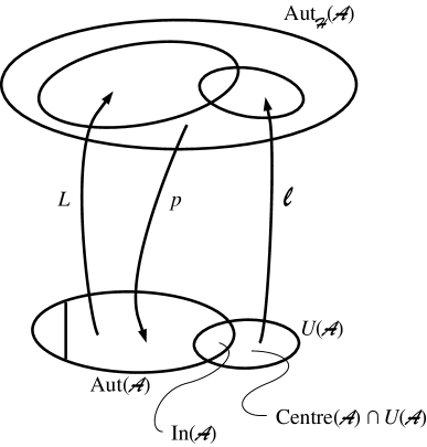
Figure 1: Lifting automorphisms and unitaries

Let us denote the elements of ${}^{M}\left(U(1)_{V}\times U(1)_{A}\right)$ by $(U_{V},U_{A})=(\exp(i\theta_{V}(x)),\exp(i\theta_{A}(x)))$. Their action on a spinor $\psi_{t}(x)$ is given by

$$R(U_{V},U_{A})=\pmatrix{\exp\left\{2i\left(\theta_{V}1_{4}+\theta_{A}\gamma_{5}\right)\right\}&0\cr 0&\exp\left\{-2i\left(\theta_{V}1_{4}+\theta_{A}\gamma_{5}\right)\right\}},$$ (55)

$$\exp\left\{\pm 2i\left(\theta_{V}1_{4}+\theta_{A}\gamma_{5}\right)\right\}=\exp\left\{\pm 2i\left(\theta_{V}-\theta_{A}\right)\right\}\,\frac{1-\gamma_{5}}{2}\,+\,\exp\left\{\pm 2i\left(\theta_{V}+\theta_{A}\right)\right\}\,\frac{1+\gamma_{5}}{2}\,.$$ (56)

While the Maxwell gauge transformation $U_{V}$ ($\cdot_{V}$ for vectorial) comes from a unitary, $R(U_{V},1)=\ell(u_{V})$, the chiral transformation $U_{A}$ ($\cdot_{A}$ for axial) is an uninvited guest. Connes writes him a letter of invitation by doubling fermions once again. He defines a new spectral triple:

$${\cal A}_{t}={\cal C}^{\infty}(M)\otimes\left({\mathbb{C}}_{L}\oplus{\mathbb{C}}_{R}\right)\owns(a_{L},a_{R}),$$ (57)

$${\cal H}_{t}={\cal L}^{2}({\cal S})\otimes{\mathbb{C}}^{4}\ \owns\psi_{t}=\pmatrix{\psi_{L}\cr\psi_{R}\cr\psi^{c}_{L}\cr\psi_{R}^{c}},\quad\rho_{t}(a_{L},a_{R})=\pmatrix{a_{L}1_{4}&0&0&0\cr 0&a_{R}1_{4}&0&0\cr 0&0&\bar{a}_{L}1_{4}&0\cr 0&0&0&\bar{a}_{R}1_{4}},$$ (58)

$${\cal D}_{t}=\pmatrix{{\,\hbox{$\partial\!\!\!/$}}&0&0&0\cr 0&{\,\hbox{$\partial\!\!\!/$}}&0&0\cr 0&0&{\,\hbox{$\partial\!\!\!/$}}&0\cr 0&0&0&{\,\hbox{$\partial\!\!\!/$}}},$$ (59)

$$J_{t}=\pmatrix{0&-1&0&0\cr 1&0&0&0\cr 0&0&0&1\cr 0&0&-1&0}\otimes\pmatrix{0&0&1&0\cr 0&0&0&1\cr 1&0&0&0\cr 0&1&0&0}\circ\,{\rm c\ c},$$ (60)

$$\chi_{t}=\gamma_{5}\otimes\pmatrix{-1&0&0&0\cr 0&1&0&0\cr 0&0&-1&0\cr 0&0&0&1}.$$ (61)

This second doubling is to disentangle left- and right-handed fermions and it is an old friend from Euclidean Lagrangian field theory with chiral fermions. Like the first doubling is does not add new degrees of freedom: at the end of the day and after passage to the Minkowskian, half of the fermions are projected out by imposing $\chi_{t}\psi_{t}=\psi_{t}.$

Real, even spectral triples are natural in the sense that the tensor product of two triples $({\cal A}_{i},{\cal H}_{i},{\cal D}_{i},J_{i},\chi_{i})$, $i=1,2$ of even dimensions $d_{1}$ and $d_{2}$ is a triple $({\cal A}_{t},{\cal H}_{t},{\cal D}_{t},J_{t},\chi_{t})$ of dimension $d_{1}+d_{2}$. This tensor product is defined by

$${\cal A}_{t}={\cal A}_{1}\otimes{\cal A}_{2},\quad{\cal H}_{t}={\cal H}_{1}\otimes{\cal H}_{2},$$ (62)

$${\cal D}_{t}={\cal D}_{1}\otimes 1_{2}\ +\ \chi_{1}\otimes{\cal D}_{2},$$ (63)

$$J_{t}=J_{1}\otimes J_{2},\quad\chi_{t}=\chi_{1}\otimes\chi_{2}.$$

The second obvious choice for the Dirac operator, ${\cal D}_{1}\otimes\chi_{2}\ +\ 1_{1}\otimes{\cal D}_{2}$, is unitarily equivalent to the first one. After this second doubling, apparently we are in presence of such a tensor product: the first triple describes 4-dimensional spacetime,

$$\left({\cal C}^{\infty}(M),{\cal L}^{2}({\cal S}),{\,\hbox{$\partial\!\!\!/$}},C,\gamma_{5}\right),$$ (64)

the second describes the 0-dimensional two-point space,

$${\cal A}_{f}={\mathbb{C}}_{L}\oplus{\mathbb{C}}_{R}\owns(a_{L},a_{R}),\quad{\cal H}_{f}={\mathbb{C}}^{4},\quad\rho_{f}(a_{L},a_{R})=\pmatrix{a_{L}&0&0&0\cr 0&a_{R}&0&0\cr 0&0&\bar{a}_{L}&0\cr 0&0&0&\bar{a}_{R}},$$ (65)

$${\cal D}_{f}=0,\quad J_{f}=\pmatrix{0&0&1&0\cr 0&0&0&1\cr 1&0&0&0\cr 0&1&0&0}\circ{\rm c\ c},\quad\chi_{f}=\pmatrix{-1&0&0&0\cr 0&1&0&0\cr 0&0&-1&0\cr 0&0&0&1}.$$ (66)

We have indicated the second triple by the subscript $\cdot_{f}$ (for finite) rather than by $\cdot_{2}$. Since the Dirac operator ${\cal D}_{f}$ vanishes the two points are separated by an infinite distance according to Connes’ distance formula (14). We want to make this distance finite. The most general finite Dirac operator commuting with $J_{f}$ and anticommuting with $\chi_{f}$ is:

$${\cal D}_{f}=\pmatrix{0&m&0&0\cr\bar{m}&0&0&0\cr 0&0&0&\bar{m}\cr 0&0&m&0}, m\in{\mathbb{C}}.$$ (67)

Now the distance between the points is $1/|m|$. On the other hand ${\cal D}_{t}={\,\hbox{$\partial\!\!\!/$}}\otimes 1_{4}\ +\ \gamma_{5}\otimes{\cal D}_{f}$ is precisely the free massive Euclidean Dirac operator.

The tensor product of the above triples describes the two-sheeted universe, with two flat sheets at constant distance. We are eager to see this free Dirac operator ${\cal D}_{t}$ fluctuate.

$$\left(L(\varphi),\ell(u_{L},u_{R})\right){\cal D}_{t}\left(L(\varphi),\ell(u_{L},u_{R})\right)^{-1}=\pmatrix{\tilde{\,\hbox{$\partial\!\!\!/$}}_{L}&\Phi\gamma_{5}&0&0\cr\bar{\Phi}\gamma_{5}&\tilde{\,\hbox{$\partial\!\!\!/$}}_{R}&0&0\cr 0&0&C\tilde{\,\hbox{$\partial\!\!\!/$}}_{L}C^{-1}&\bar{\Phi}\gamma_{5}\cr 0&0&\Phi\gamma_{5}&C\tilde{\,\hbox{$\partial\!\!\!/$}}_{R}C^{-1}},$$ (68)

with two gauge bosons

$$\tilde{A}_{L\tilde{\mu}}={\textstyle\frac{1}{i}}u_{L}\tilde{\partial}_{\tilde{\mu}}u_{L}^{-1}=\,\frac{{\partial}\theta_{L}}{{\partial}\tilde{x}^{\tilde{\mu}}},\quad\tilde{A}_{R\tilde{\mu}}={\textstyle\frac{1}{i}}u_{R}\tilde{\partial}_{\tilde{\mu}}u_{R}^{-1}=\,\frac{{\partial}\theta_{R}}{{\partial}\tilde{x}^{\tilde{\mu}}},$$ (69)

their corresponding covariant derivatives,

$$\tilde{\,\hbox{$\partial\!\!\!/$}}_{L}=i\hbox{$\tilde{e}^{-1\,\tilde{\mu}}$}_{a}\gamma^{a}\left[\tilde{\partial}_{\tilde{\mu}}+s(\tilde{\omega}_{\tilde{\mu}})-2i\tilde{A}_{L\tilde{\mu}}\right],\quad\tilde{\,\hbox{$\partial\!\!\!/$}}_{R}=i\hbox{$\tilde{e}^{-1\,\tilde{\mu}}$}_{a}\gamma^{a}\left[\tilde{\partial}_{\tilde{\mu}}+s(\tilde{\omega}_{\tilde{\mu}})-2i\tilde{A}_{R\tilde{\mu}}\right],$$ (70)

and as star guest: the Higgs boson

$$\Phi=m+u_{L}^{2}mu_{R}^{-2}.$$ (71)

Connes has generalized the exterior derivative to arbitrary spectral triples and in his sense $\Phi$ is a connection 1-form describing parallel transport between the two sheets. Its curvature vanishes. In the first stroke the metric, the two gauge bosons and the Higgs are promoted to dynamical variables with arbitrary curvature. According to Connes’ distance formula (14), this new kinematics now describes two sheets with arbitrary but identical metric and with variable separation $1/|\Phi|$. In the second stroke the spectral action produces (in addition to the familiar dynamics of metric and gauge bosons) the Klein-Gordon action for the Higgs, covariant with respect to the gauge bosons, and the quartic Higgs potential, that breaks $U(1)_{L}\times U(1)_{R}$ spontaneously down to $U(1)_{A}$. The Yukawa couplings, necessary to allow us to view the fermion mass $m$ as generated by this spontaneous symmetry breaking, stem from the fluctuation total Dirac operator ${\cal D}_{t}$, equation (68), and they have a natural interpretation as covariant derivative with respect to a transport between the two sheets. The Higgs is celebrated as star guest because he was not invited to this party, a party, that rehabilitates the entire Higgs mechanism.

Physically, the model contains two gauge bosons, a massive one with axial couplings and a massless one with vector couplings. For this reason Connes & Lott [14] called this model ‘chiral electrodynamics’. Its initial setting is that of a left-right symmetric model with left- and right-handed gauge bosons. However the Higgs sector, on which there is no handle in Connes’ setting, decides that the eigenstates of the mass matrix of the gauge bosons have vector and axial couplings. Consequently parity is not broken spontaneously. This is a general feature in noncommutative geometry [15].

At this point one remark is in order. Our initial motivation was a certain balance between automorphisms and unitaries on the one side and lifted automorphisms on the other side. Now we have a new phenomenon, there are automorphisms close to the identity that cannot be lifted, see figure. Indeed locally, Aut(${\cal A}_{t}$) = Diff($M)\times$Diff($M)\,\owns\,(\varphi_{L},\varphi_{R}).$ However only automorphisms satisfying $\varphi_{L}=\varphi_{R}$ can be lifted to the Hilbert space. This phenomenon guarantees that the massive Dirac action remains local in the sense of field theory, i.e. the Lagrangian only contains products of fields and of a finite number of their derivatives at the same spacetime point.

The finite spectral triple of the two-point space still has one short coming, it does not satisfy the first order axiom. There are two ways to fix this problem: We may minimally modify the representation such that it becomes vector-like in the antiparticle sector, e.g.,

$${\cal A}_{f}={\mathbb{C}}\oplus{\mathbb{C}}\owns(a,b),\quad\rho_{f}(a,b)=\pmatrix{a&0&0&0\cr 0&\bar{b}&0&0\cr 0&0&b&0\cr 0&0&0&b}.$$ (72)

Then after the fluctuation of the metric, the charge quantisation is less restrictive, $q=-2,0,+2$. This possibility is realized in the standard model in the lepton sector. The second possibility is to enlarge the algebra by adding a third factor, for example another ${\mathbb{C}}$, and represent it vectorially,

$${\cal A}_{f}={\mathbb{C}}\oplus{\mathbb{C}}\oplus{\mathbb{C}}\owns(a,b,c),\quad\rho_{f}(a,b,c)=\pmatrix{a&0&0&0\cr 0&b&0&0\cr 0&0&\bar{c}&0\cr 0&0&0&\bar{c}}.$$ (73)

In the standard model, $c$ will be the colour. We have noticed above that there may be automorphisms close to the identity that cannot be lifted to the Hilbert space. Now, this last spectral triple has unitaries close to the identity that are lifted to the identity. Indeed, $U({\cal A}_{f})=U(1)^{3}$, but $\ell(U({\cal A}_{f}))=U(1)^{2}$. Also note that this last spectral triple alone does not satisfy the Poincaré duality, it must be accompanied by another triple, e.g. the former one.

6 The standard model

So far our spectral triples were commutative. Connes’ geometry never uses this property and develops its full power in the noncommutative case. For instance, close to the identity, Aut$({{\mathbb{H}}})=U({{\mathbb{H}}})=SU(2)$ for the noncommutative algebra ${{\mathbb{H}}}$ of quaternions and there is no need to introduce a central extension $\ell$. From the physical point of view noncommutative triples are welcome because they offer us spontaneously broken non-Abelian Yang-Mills theories. For these applications, it is sufficient to consider only mildly noncommutative triples: tensor products of the infinite dimensional commutative triple describing 4-dimensional spacetime with a finite dimensional noncommutative triple, ‘the internal space’. We call such tensor products almost commutative spaces. Madore [16] uses the word Kaluza-Klein spaces because they have the geometrical interpretation of a direct product of a 4-dimensional manifold with a discrete point set [17] as the two sheeted universe.

Only very few Yang-Mills-Higgs models can be formulated as almost commutative geometries [18] and can thereby be viewed as fluctuations of general relativity. We cannot believe that it is pure coincidence that the intricate standard model of electro-weak and strong forces is among these very few models. The weak force breaks parity, however parity cannot be broken spontaneously in Connes’ approach [15] and must therefore be broken explicitly in the finite dimensional triple. The simplest way to do so is to choose $a_{L}$ and $a_{R}$ in algebras of different dimensions, say $\dim{\cal A}_{L}>\dim{\cal A}_{R}$. As immediate consequence parity will then be maximally broken by purely left-handed gauge bosons as in the standard model.

Here is its internal space: The algebra is chosen as to reproduce $SU(2)\times U(1)\times SU(3)$ as subgroup of $U({\cal A})$,

$${\cal A}_{f}={{\mathbb{H}}}\oplus{\mathbb{C}}\oplus M_{3}({\mathbb{C}})\,\owns\,(a,b,c).$$ (74)

The internal Hilbert space is copied from the Particle Physics Booklet [19] as given in equations (1),(2),

$${\cal H}_{L} = \left({\mathbb{C}}^{2}\otimes{\mathbb{C}}^{N}\otimes{\mathbb{C}}^{3}\right)\ \oplus\ \left({\mathbb{C}}^{2}\otimes{\mathbb{C}}^{N}\otimes{\mathbb{C}}\right),$$ (75)

$${\cal H}_{R} = \left({\mathbb{C}}^{N}\otimes{\mathbb{C}}^{3}\right)\ \oplus\ \left({\mathbb{C}}^{N}\otimes{\mathbb{C}}^{3}\right)\ \oplus\ \left({\mathbb{C}}\otimes{\mathbb{C}}^{N}\otimes{\mathbb{C}}\right).$$ (76)

In each summand, the first factor denotes weak isospin doublets or singlets, the second denotes $N$ generations, $N=3$, and the third denotes colour triplets or singlets. Let us choose the following basis of ${\cal H}_{f}={\cal H}_{L}\oplus{\cal H}_{R}\oplus{\cal H}^{c}_{L}\oplus{\cal H}^{c}_{R}={\mathbb{C}}^{90}$:

$$\pmatrix{u\cr d}_{L},\ \pmatrix{c\cr s}_{L},\ \pmatrix{t\cr b}_{L},\ \pmatrix{\nu_{e}\cr e}_{L},\ \pmatrix{\nu_{\mu}\cr\mu}_{L},\ \pmatrix{\nu_{\tau}\cr\tau}_{L};$$ (77)

(78)

$$\matrix{u_{R},\cr d_{R},}\quad\matrix{c_{R},\cr s_{R},}\quad\matrix{t_{R},\cr b_{R},}\quad e_{R},\quad\mu_{R},\quad\tau_{R};$$ (79)

(80)

$$\pmatrix{u\cr d}^{c}_{L},\ \pmatrix{c\cr s}_{L}^{c},\ \pmatrix{t\cr b}_{L}^{c},\ \pmatrix{\nu_{e}\cr e}_{L}^{c},\ \pmatrix{\nu_{\mu}\cr\mu}_{L}^{c},\ \pmatrix{\nu_{\tau}\cr\tau}_{L}^{c};$$ (81)

(82)

$$\matrix{u_{R}^{c},\cr d_{R}^{c},}\quad\matrix{c_{R}^{c},\cr s_{R}^{c},}\quad\matrix{t_{R}^{c},\cr b_{R}^{c},}\quad e_{R}^{c},\quad\mu_{R}^{c},\quad\tau_{R}^{c}.$$

It is the current eigenstate basis, the representation $\rho_{f}$ acting on ${\cal H}_{f}$ by

$$\rho_{f}(a,b,c):=\pmatrix{\rho_{L}&0&0&0\cr 0&\rho_{R}&0&0\cr 0&0&{\bar{\rho}^{c}_{L}}&0\cr 0&0&0&{\bar{\rho}^{c}_{R}}}$$ (83)

with

$$\rho_{L}(a):=\pmatrix{a\otimes 1_{N}\otimes 1_{3}&0\cr 0&a\otimes 1_{N}&},\quad\rho_{R}(b):=\pmatrix{b1_{N}\otimes 1_{3}&0&0\cr 0&\bar{b}1_{N}\otimes 1_{3}&0\cr 0&0&\bar{b}1_{N}},$$ (84)

$$\rho^{c}_{L}(b,c):=\pmatrix{1_{2}\otimes 1_{N}\otimes c&0\cr 0&\bar{b}1_{2}\otimes 1_{N}},\quad\rho^{c}_{R}(b,c):=\pmatrix{1_{N}\otimes c&0&0\cr 0&1_{N}\otimes c&0\cr 0&0&\bar{b}1_{N}}.$$ (85)

At this point we understand why only isospin doublets and singlets and colour triplets and singlets can be used in the fermionic representation: all other irreducible group representations cannot be extended to algebra representation. While the tensor product of two group representations is again a group representation, the tensor product of two algebra representations is not an algebra representation. The apparent asymmetry between particles and antiparticles – the former are subject to weak, the latter to strong interactions – disappears after application of the lift $\ell$ with

$$J_{f}=\pmatrix{0&1_{15N}\cr 1_{15N}&0}\circ\ {\rm complex\ conjugation}.$$ (86)

For the sake of completeness, we record the chirality as matrix

$$\chi_{f}=\pmatrix{-1_{8N}&0&0&0\cr 0&1_{7N}&0&0\cr 0&0&-1_{8N}&0\cr 0&0&0&1_{7N}}.$$ (87)

The internal Dirac operator

$${\cal D}_{f}=\pmatrix{0&{{\cal M}}&0&0\cr{{\cal M}}^{*}&0&0&0\cr 0&0&0&\bar{{\cal M}}\cr 0&0&\bar{{\cal M}}^{*}&0}$$ (88)

contains the fermionic mass matrix of the standard model,

$${{\cal M}}=\pmatrix{\pmatrix{1&0\cr 0&0}\otimes M_{u}\otimes 1_{3}\,+\,\pmatrix{0&0\cr 0&1}\otimes M_{d}\otimes 1_{3}&0\cr 0&\pmatrix{0\cr 1}\otimes M_{e}},$$ (89)

with

$$M_{u}:=\pmatrix{m_{u}&0&0\cr 0&m_{c}&0\cr 0&0&m_{t}}, M_{d}:=C_{KM}\pmatrix{m_{d}&0&0\cr 0&m_{s}&0\cr 0&0&m_{b}},$$ (90)

$$M_{e}:=\pmatrix{m_{e}&0&0\cr 0&m_{\mu}&0\cr 0&0&m_{\tau}}.$$ (91)

From the booklet we know that all indicated fermion masses are different from each other and that the Cabibbo-Kobayashi-Maskawa matrix $C_{KM}$ is non-degenerate in the sense that no quark is simultaneously mass and weak current eigenstate.

We note that Majorana masses are forbidden because of the axiom ${\cal D}_{f}\chi_{f}=-\chi_{f}{\cal D}_{f}.$ At least one neutrino must be without a right-handed piece in order to fulfil the Poincaré duality which for a finite dimensional spectral triple states that the intersection form

$$\cap_{ij}:={\rm tr}\,\left[\chi_{f}\,\rho_{f}(p_{i})\,J_{f}\rho_{f}(p_{j})J_{f}^{-1}\right]$$ (92)

must be non-degenerate. The $p_{j}$ are a set of minimal projectors of ${\cal A}_{f}$. The standard model has three minimal projectors,

$$p_{1}=(1_{2},0,0),\quad p_{2}=(0,1,0),\quad p_{3}=\left(0,0,\pmatrix{1&0&0\cr 0&0&0\cr 0&0&0}\right)$$ (93)

and the intersection form with three purely left-handed neutrinos,

$$\cap=-6\pmatrix{0&1&1\cr 1&-1&-1\cr 1&-1&0},$$ (94)

is non-degenerate. However if we add three right-handed neutrinos to the standard model, massive or not, then the intersection form,

$$\cap=-6\pmatrix{0&1&1\cr 1&-2&-1\cr 1&-1&0},$$ (95)

is degenerate and Poincaré duality fails.

The first order axiom, $[[{\cal D}_{f},\rho_{f}(a)],J_{f}\rho_{f}(\tilde{a})J_{f}^{-1}]=0$ for all $a,\tilde{a}\in{\cal A}_{f}$ requires a gauge group that commutes with the electro-weak interactions and with the fermionic mass matrix and whose fermion representation is vectorial [5].

The fluctuation of the free Dirac operator ${\cal D}_{t}$ gives rise to the minimal couplings to gravity and to the non-Abelian gauge bosons and to the Yukawa couplings to the Higgs boson that transforms like $(2,-{\textstyle\frac{1}{2}},1)$.

The spectral action $S_{CC}$ yields [4], in addition to the gravitational action, the entire bosonic action of the standard model including the entire Higgs sector with its spontaneous symmetry breaking. The constraints for the coupling constants, $g_{2}^{2}=g_{3}^{2}={\textstyle\frac{5}{3}}g_{1}^{2}=3\lambda$ occur because the Yang-Mills actions and the $\lambda|\Phi|^{4}$ term stem from the same heat kernel coefficient $f_{4}a_{4}$. After renormalisation through the big desert they yield a Higgs mass of 182 $\pm$ 17 GeV.

6.1 To gauge or not to gauge

It is a long standing problem of the standard model what symmetry of its fermion content do we gauge and which one do we not gauge and there is no general principle to answer this question. Not so in the noncommutative setting where this choice is not arbitrary. Indeed, the lifted automorphism group of the internal part of the standard model is

$${\rm Aut}_{{\cal H}_{f}}({\cal A}_{f})=SU(2)_{L}\times SU(3)_{c}\times U(N)_{qL}\times U(N)_{\ell L}\times U(N)_{uR}\times U(N)_{dR}\times U(N)_{eL},$$ (96)

close to the identity. Only the isospin $SU(2)_{L}$, the colour $SU(3)_{c}$ and two $U(1)$s in the five flavour $U(N)$s are invited guests, i.e. they are images under the lift $\ell$ of unitaries of the algebra ${\cal A}_{f}$. The subscripts indicate on which generation multiplet the $U(N)$s act, $qL$ for the $N=3$ left-handed quark doublets, $\ell L$ for the left-handed lepton doublets, $uR$ for the right-handed quarks of charge 2/3 and so forth. The natural question at this point is: For which of the 43 uninvited guests can we write letters of invitation by extending the internal algebra? The answer comes from the axioms of spectral triples, in particular from the first order axiom and Poincaré duality: only 10 additional symmetries can be gauged, one left-handed and 9 right-handed ones:

$${\cal A}_{f}=M_{2}({\mathbb{C}})\oplus{\mathbb{C}}\oplus M_{3}({\mathbb{C}})\oplus M_{N}({\mathbb{C}})\owns(a,b,c,d)$$ (97)

with three possible representations,

$$\rho_{R}(b,d):=\pmatrix{d\otimes 1_{3}&0&0\cr 0&\bar{d}\otimes 1_{3}&0\cr 0&0&\bar{b}1_{N}},$$ (98)

$$\rho_{R}(b,d):=\pmatrix{b1_{N}\otimes 1_{3}&0&0\cr 0&\bar{b}1_{N}\otimes 1_{3}&0\cr 0&0&\bar{d}},\quad{\rm or}\quad\rho_{R}(b,d):=\pmatrix{d\otimes 1_{3}&0&0\cr 0&\bar{d}\otimes 1_{3}&0\cr 0&0&\bar{d}},$$ (99)

$\rho_{L}$, $\rho_{L}^{c}$ and $\rho_{R}^{c}$ being as in the standard model. Only in the first of the three possibilities, the $U(N)$ is anomaly free. A phenomenological assessment of this extension of the standard model with maximally gauged flavour symmetry is under way.

6.2 O’Raifeartaigh’s reduction

We owe to O’Raifeartaigh [6] the intriguing observation that all hypercharges in the standard model conspire such that its group can be reduced to

$$G=SU(2)\times U(1)\times SU(3)/({\mathbb{Z}}_{2}\times{\mathbb{Z}}_{3}),$$ (100)

where

$${\mathbb{Z}}_{2}\times{\mathbb{Z}}_{3} = \{(\exp[-k_{2}2\pi i/2]1_{2},\exp[k_{2}2\pi i/2+k_{3}2\pi i/3],\exp[-k_{3}2\pi i/3]\,1_{3}),$$ (102)

$$\quad k_{2}=0,1,\ k_{3}=0,1,2\}$$

is the kernel of the representation of the standard model on ${\cal H}_{L}\oplus{\cal H}_{R}$ given by equations (1) and (2). The map

$$j:SU(2)\times U(1)\times SU(3) \longrightarrow SU(2)\times U(3)$$ (103)

$$(s_{2},u_{1},s_{3}) \longrightarrow (s_{2},u_{1}s_{3})$$ (104)

$$(s_{2},(\det u_{3})^{1/3},(\det u_{3})^{-1/3}u_{3}) \longleftarrow (s_{2},u_{3})$$ (105)

defines an isomorphism from $G$ to $SU(2)\times U(3)/{\mathbb{Z}}_{2}$. The latter form is useful to reduce the group of unitaries $U({\cal A}_{f})=SU(2)\times U(1)\times U(3)$ to $SU(2)\times U(3)$ by use of the unimodularity condition. We write [7] this condition as an injection

$$m:SU(2)\times U(3) \longrightarrow SU(2)\times U(1)\times U(3)=U({\cal A}_{f})$$ (106)

$$(s_{2},u_{3}) \longmapsto (s_{2},\det u_{3},u_{3}).$$ (107)

Then the group representation of the standard model on ${\cal H}_{L}\oplus{\cal H}_{R}$ is $\ell\circ m\circ j$. Imposing the unimodularity condition is equivalent to imposing vanishing gauge and mixed gravitational-gauge anomalies [20]. Still today the unimodularity condition remains a disturbing feature of the noncommutative formulation of the standard model but we must acknowledge that this condition exists at all. It exists thanks to the conspiration of the hypercharges that allows the ${\mathbb{Z}}_{3}$ reduction. Now what about the ${\mathbb{Z}}_{2}?$ Remember the charge quantisation $q=\pm 2$ in section 4. Its origin is clear. Although the algebra representation $\rho$ is faithful by definition, the group representation $\ell$ is not. Its kernel is another ${\mathbb{Z}}_{2}\subset U({\cal A})$. An immediate calculation shows that O’Raifeartaigh’s ${\mathbb{Z}}_{2}$ maps to this ${\mathbb{Z}}_{2}\subset U({\cal A})$:

$$1_{{\cal H}_{L}\oplus{\cal H}_{R}}.$$ (108)

$$\uparrow\ \ell$$ (109)

$$(\exp[-k_{2}2\pi i/2]1_{2},\exp[k_{2}6\pi i/2],\exp[k_{2}2\pi i/2]\,1_{3}) \!\!\!\!\!\!\!\!\!\!\!\!\!\!\!\!\!\!=\exp[k_{2}i\pi](1_{2},1,1_{3})$$ (110)

$$\uparrow\ m$$ (111)

$$(\exp[-k_{2}2\pi i/2]1_{2},\exp[k_{2}2\pi i/2]\,1_{3})$$ (112)

$$\uparrow\ j$$ (113)

$$(\exp[-k_{2}2\pi i/2]1_{2},\exp[k_{2}2\pi i/2+k_{3}2\pi i/3],\exp[-k_{3}2\pi i/3]\,1_{3})$$ (114)

Conversely, if the hypercharges had not conspired in favour of O’Raifeartaigh’s ${\mathbb{Z}}_{2}$ then the standard model would not fit in Connes’ geometrical frame.

7 Dreams

It is allowed to dream of a truly noncommutative spectral triple with an algebra ${\cal A}$ whose low energy ‘approximation’ $E\ll\Lambda$ is the almost commutative ${\cal A}_{t}={\cal C}^{\infty}(M)\otimes({\cal H}\oplus{\mathbb{C}}\oplus M_{3}({\mathbb{C}}))$. ‘Truly noncommutative’ means that all automorphisms are inner, Aut$({\cal A})=$  In$({\cal A})=U({\cal A})$. In this situation the two lifts $L$ and $\ell$ coincide, see figure, and the unification of gravity and Yang-Mills forces would be perfect. The opposite extreme is the commutative algebra of pure gravity, ${\cal C}^{\infty}(M)$, which has no inner automorphisms at all. The lifted automorphisms of the truly noncommutative triple would contain the spin cover of the Lorentz group only approximately at low energies and we could expect manifestations of the noncommutative nature of spacetime in the form of violations of Lorentz invariance above $10^{17}$ GeV. Amelino-Camelia has three convincing arguments [21] that the experimental observation of such violations might be possible within the next ten years. The dream continues with a generalization of the group of lifted automorphisms of the truly noncommutative triple to a Hopf algebra. And this Hopf algebra would be related to a new quantum field theory which includes gravity and which reduces to ordinary quantum field theory at low energies. The mirage of this Hopf algebra at low energies would be the one recently discovered by Connes, Moscovici and Kreimer [22].

As always, I am indebted to Raymond Stora. From him I learnt the symmetric gauge some 17 years ago. It is also a pleasure to acknowledge help and advice by Samuel Friot, Bruno Iochum, Daniel Kastler, Serge Lazzarini, Carlo Rovelli, Daniel Testard and Antony Wassermann.

References

• [1] A. Connes, Noncommutative Geometry, Academic Press (1994)
• [2] A. Connes, Noncommutative geometry and reality, J. Math. Phys. 36 (1995) 6194
• [3] A. Connes, Gravity coupled with matter and the foundation of noncommutative geometry, hep-th/9603053, Comm. Math. Phys. 155 (1996) 109
• [4] A. Chamseddine & A. Connes, The spectral action principle, hep-th/9606001, Comm. Math. Phys.186 (1997) 731
• [5] R. Asquith, Non-commutative geometry and the strong force, hep-th/9509163, Phys. Lett. B 366 (1996) 220
• [6] L. O’Raifeartaigh, Group Structure of Gauge Theories, Cambridge University Press 1986
• [7] S. Lazzarini & T. Schücker, Standard model and unimodularity condition, hep-th/9801143, in the proceedings of the Workshop on Quantum Groups, Palermo, 1997, ed.: Daniel Kastler, Nova Science, 1999
• [8] L. Carminati, B. Iochum & T. Schücker, Noncommutative Yang-Mills and noncommutative relativity: A bridge over troubled water, hep-th/9706105, Eur. Phys. J. C8 (1999) 697
• [9] J. C. Várilly & J. M. Gracia-Bondía, Connes’ noncommutative differential geometry and the standard model, J. Geom. Phys. 12 (1993) 223
D. Kastler, A detailed account of Alain Connes’ version of the standard model in non-commutative geometry, I and II, Rev. Math. Phys. 5 (1993) 477 D. Kastler, A detailed account of Alain Connes’ version of the standard model in non-commutative geometry, III, Rev. Math. Phys. 8 (1996) 103
D. Kastler & T. Schücker, A detailed account of Alain Connes’ version of the standard model in non-commutative geometry, IV, Rev. Math. Phys., 8 (1996) 205
J. Madore, An Introduction to Noncommutative Differential Geometry and its Physical Applications, Cambridge University Press (1995)
G. Landi, An Introduction to Noncommutative Spaces and their Geometry, hep-th/9701078, Springer, Heidelberg (1997)
C. P. Martín, J. M. Gracia-Bondía & J. C. Várilly, The standard model as a noncommutative geometry: the low mass regime, hep-th/9605001, Phys. Rep. 294 (1998) 363
J. C. Várilly, Introduction to noncommutative geometry, physics/9709045, to appear in the proceedings of the EMS Summer School on Noncommutative Geometry and Applications, Portugal, 1997, ed.: P. Almeida
T. Schücker, Geometries and forces, hep-th/9712095, to appear in the proceedings of the EMS Summer School on Noncommutative Geometry and Applications, Portugal, 1997, ed.: P. Almeida
D. Kastler, Noncommutative geometry and basic physics, to appear in the proceedings of the Schladming Winter School 1999, ed.: H. Grosse, Springer Heidelberg
D. Kastler, Noncommutative Geometry and fundamental physical interactions: the Lagrangian level, in the J. Math. Phys. 2000 issue: ‘Mathematical Physics: Past and Future’
• [10] J. M. Gracia-Bondía, J. C. Várilly & H. Figueroa, Elements of Noncommutative Geometry, Birkhäuser (2000)
• [11] J.-P. Bourguignon & P. Gauduchon, Spineurs, opérateurs de Dirac et variations de métriques, Comm. Math. Phys. 144 (1992) 581
• [12] Samuel Friot, Géométrie commutative: unification Maxwell-Einstein, DEA thesis, Marseille, 2000
• [13] G. Landi & C. Rovelli, Gravity from Dirac eigenvalues, gr-qc/9708041, Mod. Phys. Lett. A13 (1998) 479
• [14] A. Connes & J. Lott, The metric aspect of noncommutative geometry, in the proceedings of the 1991 Cargèse Summer Conference, eds.: J. Fröhlich et al., Plenum Press (1992)
• [15] B. Iochum & T. Schücker, A left-right symmetric model à la Connes-Lott, hep-th/9401048, Lett. Math. Phys. 32 (1994) 153
F. Girelli, Left-right symmetric models in noncommutative geometry?, to be published
• [16] J. Madore, Modification of Kaluza Klein theory, Phys. Rev. D 41 (1990) 3709
• [17]  for recent examples of discrete spaces see,
B. Iochum, T. Krajewski & P. Martinetti, Distances in finite spaces from noncommutative geometry, hep-th/9912217, to appear in J. Geom. Phys.
• [18] B. Iochum & T. Schücker, Yang-Mills-Higgs versus Connes-Lott, hep-th/9501142, Comm. Math. Phys. 178 (1996) 1
M. Paschke & A. Sitarz, Discrete spectral triples and their symmetries, q-alg/9612029, J. Math. Phys. 39 (1998) 6191
T. Krajewski, Classification of finite spectral triples, hep-th/9701081, J. Geom. Phys. 28 (1998) 1
• [19] The Particle Data Group, Particle Physics Booklet and http://pdg.lbl.gov
• [20] E. Alvarez, J. M. Gracia-Bondía & C. P. Martín, Anomaly cancellation and the gauge group of the Standard Model in Non-Commutative Geometry, hep-th/9506115, Phys. Lett. B364 (1995) 33
• [21] G. Amelino-Camelia, Are we at the dawn of quantum gravity phenomenology? Lectures given at 35th Winter School of Theoretical Physics: From Cosmology to Quantum Gravity, Polanica, Poland, 1999, gr-qc/9910089
• [22] A. Connes & H. Moscovici, Hopf Algebra, cyclic cohomology and the transverse index theorem, Comm. Math. Phys. 198 (1998) 199
D. Kreimer, On the Hopf algebra structure of perturbative quantum field theories, q-alg/9707029, Adv. Theor. Math. Phys. 2 (1998) 303
A. Connes & D. Kreimer, Renormalization in quantum field theory and the Riemann-Hilbert problem. 1. The Hopf algebra structure of graphs and the main theorem, hep-th/9912092, Comm. Math. Phys. 210 (2000) 249
A. Connes & D. Kreimer, Renormalization in quantum field theory and the Riemann-Hilbert problem. 2. the beta function, diffeomorphisms and the renormalization group, hep-th/0003188