Holography in an Early Universe with Asymmetric Inflation

Elcio Abdalla and L. Alejandro Correa-Borbonet

Instituto de Física, Universidade de São Paulo,

C.P.66.318, CEP 05315-970, São Paulo, Brazil

Abstract

We discuss the validity of the holographic principle in a $(4+n)$ dimensional universe in an asymmetric inflationary phase.

PACS number(s): 98.80.Cq 04.50.+h

Recently a new possible solution to the hierarchy problem has been proposed [1], where the fundamental Planck scale goes down to the level of the Tev region, provided that there are compact extra dimensions where gravitationals fields propagate. In such a case, the size of these extra dimensions should be in the submillimiter scale in order to conform to the phenomenological constraints. Indeed, using Gauss’s law in $(4+n)$ dimensions it is possible to relate the Planck scale in the $(4+n)$ dimensional theory($M_{*}$) with that of the $4$-dimensional theory ($M_{Pl}$) by means of the size of the $n$ compactified dimensions ($b_{0}$). It is easy to find [5]

$$M^{2}_{Pl}=(b_{0})^{n}M^{n+2}_{*}$$ (1)

Assuming the usual value $M_{Pl}\simeq 10^{19}$ GeV and $M_{*}\simeq 1$ TeV, we find $b_{0}\sim 10^{-17+\frac{30}{n}}$ cm. For $n=2$ we obtain the (reasonable) value $b_{0}\simeq 1$ mm. We would thus find deviation from Newtonian gravitation in a range within experimental search in the near future.

There are several papers discussing the theoretical and phenomenological aspects of this idea [2]. From the fundamental point of view, gravity can propagate freely around the whole set of dimensions in the submillimeter region, but the Standard Model (SM) fields get confined in the $4$-dimensional world. This is feasible if we consider that the SM fields are localized on a $3$-brane immersed in the higher-dimensional space, as in the case of D-branes occurring in type I/II string theory[3],[4]. Thus a very attractive model of early universe has been proposed [5], and the underlying cosmology that occurs for small extra dimensions can be of wide interest.

In this model the dynamics of the dimensions as described by the Einstein equations is the central question. They are divided in a (so called wall) four dimensional world, and the $n$-internal dimensions. In concrete terms, the picture proposed is that of an early inflationary era followed by a long epoch where the scale factor of the brane-universe undergoes a slow contraction while the internal dimensions continue to expand towards their stabilized value. When the contraction ends the universe goes asymptotically to the radiation dominated behaviour as described by the FRW model. Although details of the dynamics underlying the transition are not known, a reasonable alternative explanation of the dynamics leading to the Cosmological standard model may arises.

On the other hand, we have witnessed a great activity on the holographic principle [6, 7] which states that all information about physical processes in cosmology can be stored on the surface enclosing the physical universe. This idea has received strong support from another conjeture known as the AdS/CFT correspondence[8]. The conjetured equivalence between Supergravity on D-dimensional AdS space and conformal field theory on the $(D-1)$-dimensional boundary has been proven very useful to gain information about supergravity in the bulk from knowledge about its boundary. Moreover, the holographic principle has been extended to cosmology and there have been many attempts to apply different formulations of this principle to various cosmological models.

In this paper we will try to check the compatibility of the holographic principle with the cosmological model proposed by Arkani-Hamed et al [5]. Specifically the cosmological version of the holographic principle proposed by Fischler and Susskind[9] will be checked. Here we will restrict to the study of the contraction epoch with two extra dimensions, in agreement with the afore mentioned phenomenological constraints.

The evolution of the scale factors $a(t)$ corresponding to the $3$-dimensional physical (observable) space, and $b(t)$, corresponding to the internal dimensions, is described by the Einstein equations as given by[5]

$$6H^{2}_{a}+2H^{2}_{b}+12H_{a}H_{b}=\frac{V}{M^{4}_{*}b^{2}},$$ (2)

$$\frac{\ddot{b}}{b}+H^{2}_{b}+3H_{b}H_{a}=\frac{1}{M^{4}_{*}b^{2}}(\frac{V}{2}-\frac{b}{8}\frac{\partial V}{\partial b}),$$ (3)

$$\frac{\ddot{a}}{a}+2H^{2}_{a}+2H_{b}H_{a}=\frac{b}{8M^{4}_{*}b^{2}}\frac{\partial V}{\partial b}.$$ (4)

where we have introduced the Hubble parameters $H_{a}\equiv\dot{a}/a$ and $H_{b}\equiv\dot{b}/b$ for the two scale factors, the overdot denoting the derivative with respect to $t$. Here, $V$ is the stabilizing potential, which is a function of the scale factor $b$. These quantities are in the socalled string (brane) frame. The reason is that the kinematics in this frame is automatically expressed in terms of the units measured by the observers which live on the wall.

This system has been obtained from the original Einstein equations after neglecting the energy density $\rho$ and pressure $p$ (see Eq($57$) in [5]). Using the COBE data we can prove that values of $\rho$ and $p$ are much smaller than the potential $V$. This potential, in the semiclassical limit, may be viewed as an expansion in inverse powers of the scale factor $b(t)$. Simplifying, it has been taken as being a monomial form, $V=Wb^{-p}$, where $W$ is a dimensionful parameter.

These equations can be solved exactly. Defining

$$a=a_{i}e^{\alpha(t)}\;\;\;\;\;\;b=b_{i}e^{\beta(t)}$$ (5)

and going to the new time variable

$$d\tau=-e^{-3\alpha-2\beta}dt$$ (6)

the previous system, after some algebra, can be reduced to a functional constraint equation [5]

$$4\alpha+\frac{4p}{4+p}\beta=C_{1}+C_{2}\tau$$ (7)

together with a simple first order differential equation,

$$X^{\prime 2}=\frac{\Delta}{4}\omega e^{X}+\frac{3(4+p)^{2}}{32}C^{2}_{2}$$ (8)

where

$$X=6\alpha+(2-p)\beta$$ (9)

and $C_{1}$, $C_{2}$ are integration constants. The other two parameters that appear in the system are $\Delta=8-8p-p^{2}$ , $\omega=\frac{W}{M^{4}_{*}b^{2+p}_{i}}$. The prime denote the derivative with respect to $\tau$.

The solutions of the system take different form, controlled by whether $C_{2}$ vanishes or not, and by the value of $\Delta$. It is found that the solutions can be classified in four types:

$$(1)\,\Delta=0;\quad(2)\,\Delta>0,C_{2}=0;\quad(3)\,\Delta>0,C_{2}<0;\quad(4)\,\Delta<0,C_{2}<0$$ (10)

The critical value $\Delta=0$ corresponds to $p\simeq 0.899$. In this case the solution is

$$a=a_{i}(\frac{t}{t_{i}})^{k}\quad,$$ (11)

$$b=b_{i}(\frac{t}{t_{i}})^{l}\quad,$$ (12)

with $k=-0.1266$ and $l=0.69$. Such values satisfy the two algebraic equations, namely

$$3k+2l=1\quad,$$ (13)

and

$$3k^{2}+2l^{2}=1\quad,$$ (14)

implying that in this era the solution describes a Kasner universe.

Applying the F-S criteria for anisotropic universes the following entropy/area relation is obtained, with the bar quantities defined in the Einstein frame,

$$S/A=\frac{\bar{\sigma}(\bar{R}_{H,\bar{a}})^{3}(\bar{R}_{H,\bar{b}})^{2}}{[(\bar{a}\bar{R}_{H,\bar{a}})^{3}(\bar{b}\bar{R}_{H,\bar{b}})^{2}]^{4/5}}\quad,$$ (15)

where the comoving size of the horizon is

$$\bar{R}_{H,\bar{a}}(\bar{t})=\int^{\bar{t}}_{\bar{t}_{i}}\frac{d\bar{t}^{\prime}}{\bar{a}(\bar{t}^{\prime})},$$ (16)

and $\bar{\sigma}$ is the comoving entropy density.

In order to calculate the S/A relation $(\ref{eq:einsfram})$ we use the expression that relate the metric in the Einstein frame with the one in the string frame [5]

$$\bar{g}_{\mu\nu}=b^{2}g_{\mu\nu}\quad.$$ (17)

Using this map, we get

$$\bar{a}=ba\;\;\;\;\;\;\bar{b}=bb\;\;\;\;\;\;d\bar{t}=bdt\quad.$$ (18)

Therefore we have

$$\bar{R}_{H,\bar{a}}=R_{H,a}\;\;\;\;\;\;\;\bar{R}_{H,\bar{b}}=R_{H,b}\quad.$$ (19)

Now, the S/A relation can be rewritten as

$$S/A=\frac{1}{b^{4}}\frac{\sigma(R_{H,a})^{3}(R_{H,b})^{2}}{[(aR_{H,a})^{3}(bR_{H,b})^{2}]^{4/5}}\quad.$$ (20)

The authors of Ref [10] argued that when the Fischler-Susskind criteria is applied to inflationary cosmology the evolution of the universe should be considered after reheating. For the model of Arkani-Hamed et $al$ we will take the initial time $t_{i}$ as corresponding to the end of the de Sitter phase, because the model does not have the usual post-inflationary reheating of standard inflationary cosmology. We also should remember that the end of the de Sitter phase is the beginning of the contraction epoch.

Taking into account the scale factors $(\ref{eq:facta})$ and $(\ref{eq:factob})$ we get, after some manipulations,

$$S/A=\frac{\sigma}{a^{3}_{i}b^{6}_{i}}c_{1}t_{i}f(x),$$ (21)

where

$$c_{1}=\frac{1}{(1-k)^{3/5}}\frac{1}{(1-l)^{2/5}}=1,4873$$ (22)

and

$$f(x)=\frac{1}{x^{4l}}\frac{(x^{1-k}-1)^{3}(x^{1-l}-1)^{2}}{(x-x^{k})^{12/5}(x-x^{l})^{8/5}}\quad,$$ (23)

where $x=t/t_{i}$.

The shape of $f(x)$ is illustrated in figure 1. Using $(\ref{eq:kasner})$ it can be checked that the asymptotic value of $f(x)$ is zero. Therefore if the holographic bound holds when $f(x)$ has its maximum value, later on, the bound will be satisfied even better.

The solutions in the case $\Delta>0$($0\leq p<0.899$) and $C_{2}=0$ are similar but the corresponding powers are

$$v=-\frac{2p}{(2+p)(4+p)}\quad,$$ (24)

$$u=\frac{2}{2+p}\quad.$$ (25)

In this case the powers satisfy

$$3v+2u>1\quad.$$ (26)

Repeating the same procedure as the previous case we find for the entropy to area ratio the result

$$S/A=\frac{\sigma}{a^{3}_{i}b^{6}_{i}}c_{2}t_{i}g(x)\quad,$$ (27)

where for $p<0.899$

$$c_{2}=\frac{1}{(1-v)^{3/5}}\frac{1}{(1-u)^{2/5}}\quad,$$ (28)

$$g(x)=\frac{1}{x^{4u}}\frac{(x^{1-v}-1)^{3}(x^{1-u}-1)^{2}}{(x-x^{v})^{12/5}(x-x^{u})^{8/5}}\quad,$$ (29)

and for $p=0$ ,

$$c_{2}=1$$ (30)

$$g(x)=\frac{1}{x^{4}}\frac{(x-1)^{3/5}(ln(x))^{2/5}}{x^{8/5}}\quad.$$ (31)

In figure 2 the function $g(x)$ is shown for diferents values of the parameter $p$($0,0.5,0.7$). Also in this case the asymptotic value of $g(x)$ is zero. In figure 3 a comparation between the functions $f(x)$ and $g(x)$ is displayed.

In the case ($\Delta<0(p>0.899),C_{2}<0$)the Kasner solution applies asymptotically (see Ref [5]). In other words, the scale factors $a(t)$ and $b(t)$ take the form $(\ref{eq:facta}),(\ref{eq:factob})$ for large times. This implies that the ratio entropy/area will coincide with the $\Delta=0$ case in the remote future (see figure 4).

The last solution ($\Delta>0,C_{2}<0$) is similarly reduced to the case ($\Delta>0,C_{2}=0$). Then, the scale factors will have the powers $(\ref{eq:expv}),(\ref{eq:expu})$ and the entropy/area relation will be described by equation $(\ref{eq:entrorA})$ in the remote future.

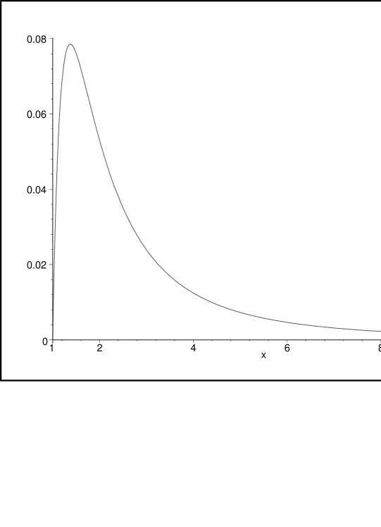
Figure 1: Function f(x) in the critical case $p=0.899.$

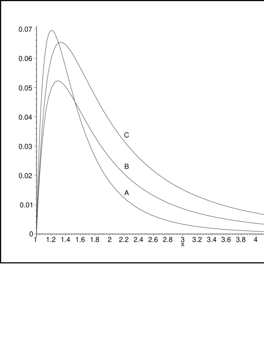
Figure 2: Function g(x) in the subcritical cases $p=0(A),0.5(B),0.7(C)$.

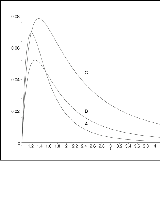
Figure 3: Comparison between the cases $p=0(A),0.5(B),0.899(C)$.

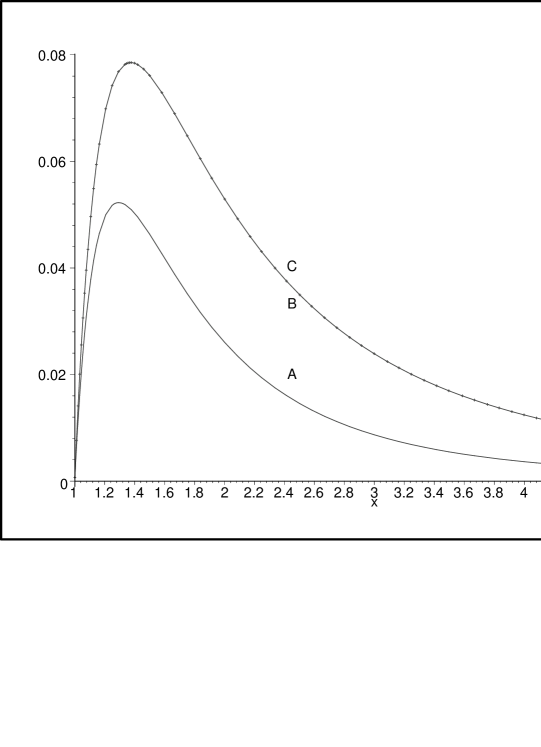
Figure 4: Comparison between the cases $p=0.5(A),0.899(B),8(C)$.

In conclusion, we have found that the holographic principle can be satisfied in the contraction epoch for the model of Arkani Hamed et $al$[5]. The entropy to area ratio has a similar asymptotic behavior for all the solutions. As this model presents some novelties for inflationary cosmology, the results that we have obtained could be useful in order to improve our understanding of the holographic principle in relation to cosmology.

ACKNOWLEDGMENT: This work was partially supported by Fundação de Amparo à Pesquisa do Estado de São Paulo (FAPESP), Conselho Nacional de Desenvolvimento Científico e Tecnológico (CNPQ) and CAPES (Ministry of Education, Brazil).

References

- [1] N. Arkani-Hamed, S. Dimopoulos and G.Dvali, Phys. Lett. B429, 263 (1998).
- [2] P. Argyres, S. Dimopoulos and J. March-Russell, Phys. Lett. B441, 96 (1998); Z. Kakushadze and S.H. Tye, Nucl. Phys. B548, 180 (1999); K. Benakli, Phy. Rev. D60, 104002 (1999); L.Randall and R. Sundrum, Nucl.Phys. B557, 79 (1999).
- [3] J. Polchinski, Phys. Rev. Lett. 75, 4724 (1995).
- [4] I. Antoniadis, N. Arkani-Hamed, S. Dimopoulos and G.Dvali, Phys. Lett. B436, 257 (1998).
- [5] N. Arkani-Hamed, S. Dimopoulos, N. Kaloper and J. March-Russell, Nucl. Phys. B567, 189 (2000).
- [6] G.’t Hooft, gr-qc/9310026.
- [7] L.Susskind, J. Math. Phys. 36, 6377 (1995).
- [8] J.M. Maldacena, Adv. Theor. Math. Phys. 2, 231 (1998); E.Witten, Adv. Theor. Math. Phys. 2, 253 (1998); S.S.Gubser, I.R. Klebanov and A. M. Polyakov, Phys. Lett. B428, 105 (1998).
- [9] W.Fischler and L. Susskind, Holography and Cosmology, hep-th/9806039.
- [10] N.Kaloper and A.Linde, Phys.Rev. D60, 103509 (1999).