[

Brane world from IIB matrices

Abstract

We have recently proposed a dynamical mechanism that may realize a flat four-dimensional space time as a brane in type IIB superstring theory. A crucial rôle is played by the phase of the chiral fermion integral associated with the IKKT Matrix Theory, which is conjectured to be a nonperturbative definition of type IIB superstring theory. We demonstrate our mechanism by studying a simplified model, in which we find that a lower-dimensional brane indeed appears dynamically. We also comment on some implications of our mechanism on model building of the brane world.

]

Introduction.—

The idea that our four-dimensional space time is realized as a brane in a non-compact higher-dimensional space time has recently attracted much attention. Through many works during the last few years, it is expected to provide natural resolutions to many long-standing problems in the Standard Model. The hierarchy problem is transmuted into a geometrical one [3], and it was further argued that the exponential dependence of the “warp” factor in the extra directions reduces the problem to a fine-tuning of order 50 [4]. The cosmological constant problem may also be resolved in such a setup [5]. It has been argued that any nonzero higher-dimensional cosmological constant is absorbed into the warp factor, and that the four-dimensional cosmological constant is automatically tuned to zero (or to a very small number). A possible obstruction to the idea (as opposed to a more conventional idea using Kaluza-Klein compactifications) is that gravity may propagate in higher dimensions and thereby contradicts the 4D Newton’s law observed in the low energy scale. However, the particular AdS-type background metric that arises naturally in such a setup allows a normalizable zero mode of the graviton bound to the brane [6]. A small correction to the 4D Newton’s law due to the continuum spectrum of massive modes is argued to be small enough to be compatible with the experimental bound. All these attractive features of the idea lead us to hope that there is a natural string-theory realization of the brane world scenario.

In Ref. [7], we have proposed a dynamical mechanism which may realize a flat four-dimensional space time as a brane in type IIB superstring theory. Obviously, such a mechanism should inevitably be of nonperturbative nature. Indeed, our mechanism was based on the IKKT version [8] of the Matrix Theory [9], namely the IIB matrix model, which is conjectured to be a nonperturbative definition of type IIB superstring theory. The model is a supersymmetric matrix model composed by ten $N\times N$ hermitian bosonic matrices and sixteen $N\times N$ hermitian fermionic matrices. The space time is represented by the eigenvalues of the bosonic matrices. The model has manifest ten-dimensional Lorentz invariance, where the bosonic and fermionic matrix elements transform as a vector and a Majorana-Weyl spinor, respectively. The integral over the fermionic matrices yields a pfaffian which is complex in general. This poses a technical difficulty known as the ‘complex action’ problem in studying the IIB matrix model by Monte Carlo simulation. Monte Carlo studies incorporating only the modulus of the pfaffian (and omitting the phase by hand) showed that the space-time becomes isotropic in ten dimensions in the large-$N$ limit [10][11]. This result suggests that the phase of the pfaffian must play a crucial rôle if a brane world naturally arises in the type IIB superstring theory. The effect of the phase is to favour configurations for which the phase becomes stationary. Such an effect has been studied within a saddle-point approximation and found to enhance lower-dimensional brane-like configurations considerably [7].

In this Letter, we demonstrate our mechanism more explicitly by studying a simplified model using Monte Carlo simulation. In this case, we find that the dominant saddle-points are given by configurations with only three-dimensional extent.

The mechanism.—

The IIB matrix model [8] is formally a zero-volume limit of $D=10$, ${\cal N}=1$, pure super Yang-Mills theory. The partition function of the IIB matrix model (and its generalizations to $D=4$ and $D=6$) can be written as

$$Z_{\rm IIB}=\int\mbox{d}A~{}\mbox{e}^{-S_{\rm b}}~{}Z_{f}[A]\ ,$$ (1)

where $S_{\rm b}=-\mbox{Tr\,}([A_{\mu},A_{\nu}]^{2})/4$, and $\Gamma[A]=-\ln Z_{f}[A]$ represents the effective action induced by integration over the fermionic matrices. The dynamical variables $A_{\mu}$ ($\mu=1,\cdots,D$) are $D$ bosonic $N\times N$ traceless hermitian matrices. Expanding $A_{\mu}$ as $A_{\mu}=\sum_{a=1}^{N^{2}-1}A_{\mu}^{a}t^{a}$ in terms of the generators $t^{a}$ $(a=1,\ldots,N^{2}-1)$ of SU($N$), the integration measure $\mbox{d}A$ is given as ${\mbox{d}}A\equiv\prod_{\mu=1}^{D}\prod_{a=1}^{N^{2}-1}dA_{\mu}^{a}$. The generators $t^{a}$ are normalized as $\mbox{Tr\,}(t^{a}t^{b})=2\delta_{ab}$.

The fermion integral $Z_{f}[A]$ is complex in general for $D=10$, $N\geq 4$ and for $D=6$, $N\geq 3$ [7][13]. We restrict ourselves to these cases in what follows. In the $D=10$ case, the fermion integral $Z_{f}[A]$ is given by the pfaffian $\mbox{Pf}\,{\cal M}$, where ${\cal M}$ is a $16(N^{2}-1)\times 16(N^{2}-1)$ complex antisymmetric matrix defined by

$${\cal M}_{a\alpha,b\beta}\equiv\mbox{Tr\,}\left(t^{a}\,(\,{\cal C}\,\Gamma_{\mu})_{\alpha\beta}[A_{\mu},t^{b}]\right)$$ (2)

regarding each of $(a\alpha)$ and $(b\beta)$ as a single index. Here, $\Gamma_{\mu}$ $(\mu=1,\ldots,10)$ are ten-dimensional Weyl-projected $16\times 16$ gamma matrices, satisfying ${\cal C}\,\Gamma_{\mu}\,{\cal C}^{\dagger}=(\Gamma_{\mu})^{\top}$ with ${\cal C}={\cal C}^{\top}$ being the unitary charge conjugation matrix. Similarly in the $D=6$ case, the fermion integral $Z_{f}[A]$ is given by the determinant $\det\,{\cal M}^{(6)}$, where ${\cal M}^{(6)}$ is a $4(N^{2}-1)\times 4(N^{2}-1)$ complex matrix defined by

$${\cal M}^{(6)}_{a\alpha,b\beta}\equiv\mbox{Tr\,}\left(t^{a}\,(\,\Gamma_{\mu}^{(6)})_{\alpha\beta}[A_{\mu},t^{b}]\right)$$ (3)

regarding each of $(a\alpha)$ and $(b\beta)$ as a single index. Here, $\Gamma_{\mu}^{(6)}$ $(\mu=1,\ldots,6)$ are six-dimensional Weyl-projected $4\times 4$ gamma matrices.

Since the fermion integral $Z_{f}[A]$ is a complex quantity for the cases under consideration, let us write it as $Z_{f}[A]=\exp(-\Gamma^{(\rm r)}-i\Gamma^{(\rm i)})$. In Ref. [7], the effect of the phase $\Gamma^{(\rm i)}$ in the path integral (1) has been studied using a saddle-point approximation, whose validity has been also discussed. The saddle-point equation for $\Gamma^{(\rm i)}$ is given by

$$\frac{\partial\,\Gamma^{(\rm i)}}{\partial A_{\mu}^{a}}=0~{}~{}~{}~{}~{}~{}~{}\forall a,\mu\ .$$ (4)

It is useful to introduce the following classification of “brane” configurations

$$\Omega_{d}=\Bigl{\{}\{A_{\mu}\}\mid\exists\,n_{\mu}^{(i)}(i=1,\cdots,D-d),\,n_{\mu}^{(i)}A_{\mu}=0\Bigr{\}}\ ,$$ (5)

where $n_{\mu}^{(i)}$ ($i=1,\cdots,D-d$) are $(D-d)$ linearly independent $D$-dimensional real vectors. Namely, $\Omega_{d}$ represents a set of configurations with less than $d$-dimensional extent. Note that $\Omega_{1}\subset\Omega_{2}\subset\cdots\subset\Omega_{D}$, where $\Omega_{D}$ is nothing but the whole configuration space of the model. In Ref. [7] we proved that all configurations in $\Omega_{D-2}$ are solutions to the saddle-point equation (4). Assuming that the configurations in $\Omega_{D-2}$ are the dominant saddle-point configurations, we still have to integrate over those configurations to determine the actual dimensionality of the space-time. In fact, the gaussian fluctuation of the phase $\Gamma^{(\rm i)}$ around the saddle-points gives a huge enhancement to the brane configurations with lower dimensionality, and this enhancement cancels exactly the entropical barrier against having such configurations. In the $D=10$ case, this provides a dynamical mechanism for the possible appearance of four-dimensional space time as a brane in ten-dimensional space time.

A simplified model.—

In order to investigate how our mechanism works, we consider a simplified model describing an integration over the saddle-point configurations. Specifically, we consider the integral

$$Z=\int\mbox{d}A~{}\mbox{e}^{-\beta F[A]-\gamma f[A]}\ ,$$ (6)

where the functions $F[A]$ and $f[A]$ are defined as

$$F[A] \equiv \sum_{\mu=1}^{D}\sum_{a=1}^{N^{2}-1}\left(\frac{\partial\,\Gamma^{(\rm i)}}{\partial A_{\mu}^{a}}\right)^{2}\ ,$$ (7)

$$f[A] \equiv \sum_{\mu=1}^{D}\sum_{a=1}^{N^{2}-1}(A_{\mu}^{a})^{2}\ .$$ (8)

Since the function $F[A]$ vanishes if and only if the configuration $\{A_{\mu}\}$ satisfies the saddle-point equation (4), the integral (6) is dominated by the saddle-point configurations in the large-$\beta$ limit. The function $f[A]$ makes the integral (6) convergent as long as the coefficient $\gamma$ is fixed to be a real positive number. In fact, the parameter $\gamma$ can be absorbed by an appropriate rescaling of $A_{\mu}^{a}$ and $\beta$. Therefore we take $\gamma=1/2$ in what follows without loss of generality. Note also that the simplified model (6) is invariant under a SO($D$) transformation $A_{\mu}\mapsto\Lambda_{\mu\nu}A_{\nu}$, where $\Lambda_{\mu\nu}\in\mbox{SO}(D)$, and a SU($N$) transformation $A_{\mu}\mapsto gA_{\mu}g^{\dagger}$, where $g\in\mbox{SU}(N)$, which are the symmetries of the original model (1).

Using the invariance of the partition function (6) under the change of variables $A_{\mu}^{a}\mapsto\lambda A_{\mu}^{a}$, one can obtain an exact relation

$$\frac{1}{2}\langle f\rangle_{\beta}-\beta\langle F\rangle_{\beta}=\frac{D}{2}(N^{2}-1)\ ,$$ (9)

where the ensemble average $\langle\,\cdot\,\rangle_{\beta}$ is defined with the partition function (6). Assuming that $\langle f\rangle_{\beta}$ goes to a constant $c$ for $\beta\rightarrow\infty$, we obtain the asymptotic behavior of $\langle F\rangle_{\beta}$ for large $\beta$ as

$$\langle F\rangle_{\beta}\sim\frac{b}{\beta}\ ,$$ (10)

where the coefficient $b$ is given as $b=c/2-D(N^{2}-1)/2$. This confirms the above claim that the integral (6) is dominated by the saddle-point configurations in the large-$\beta$ limit.

A quantity which fully characterizes the dimensionality $d$ of a given configuration can be given by the moment of inertia tensor $T$ defined by the $D\times D$ real symmetric matrix [12]

$$T_{\mu\nu}=\sum_{a=1}^{N^{2}-1}A_{\mu}^{a}A_{\nu}^{a}\,.$$ (11)

A configuration $\{A_{\mu}\}$ belongs to $\Omega_{d}$, if and only if the number of zero eigenvalues of the matrix $T$ is more than or equal to $(D-d)$. Let us denote the eigenvalues of the matrix $T$ as $\lambda_{i}$ ($i=1,\cdots,D$), where $\lambda_{1}\geq\lambda_{2}\geq\cdots\geq\lambda_{D}\geq 0$. We can determine the dimensionality of the dominant saddle-point configurations from the ensemble average of the eigenvalues $\langle\lambda_{i}\rangle_{\beta}$ in the $\beta\rightarrow\infty$ limit.

We address this issue by performing Monte Carlo simulation using a Metropolis algorithm. We create a trial configuration $\{A_{\mu}^{\prime}\}$ by replacing an element $A_{\mu}^{a}$ of the previous configuration $\{A_{\mu}\}$ with a new one generated with the probability distribution $\frac{1}{\sqrt{2\pi}}\exp[-\frac{1}{2}(A_{\mu}^{a})^{2}]$. The trial configuration is accepted with the probability $\min(1,\exp(-\beta\Delta F))$, where $\Delta F=F[A^{\prime}]-F[A]$. This procedure is repeated for all the elements of the configuration. The computational effort required for the above algorithm is of order O$(N^{8})$ per one sweep, which is much larger than that for the simulation encountered in Refs. [10, 14]. Due to this, results with high statistics are obtained only for the case of $D=6$ and $N=3$ (we have made 192,000 accepted updates for each $\beta\leq 384$ and 768,000 for $\beta=512$).

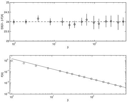
FIG. 1.: In the upper part, we plot the left hand side of eq. (9) against $\beta$ for $D=6$ and $N=3$. The dashed line represent the exact result $\frac{D}{2}(N^{2}-1)=24$. In the lower part, the function $\langle F[A]\rangle_{\beta}$ is plotted against $\beta$ in a log-log scale. The straight line represents a fit to the predicted large-$\beta$ behavior $\langle F[A]\rangle_{\beta}\sim b/\beta$.

Results.—

In the upper part of Fig. 1 we plot the left hand side of (9), which demonstrates the validity of our simulation. In the lower part of Fig. 1 we plot the average $\langle F[A]\rangle_{\beta}$ against $\beta$ in a log-log scale. The straight line represents the fit of the data for $\beta\geq 16$ to the predicted large-$\beta$ behavior (10) with $b=1.7(1)$.

Fig. 2 shows the six eigenvalues of the moment of inertia tensor $T$ as a function of $\beta$. We find that the three smallest eigenvalues $\langle\lambda_{i}\rangle_{\beta}$ ($i=4,5,6$) are monotonously decreasing with a pronounced power law behavior. Fitting the data for $\beta\geq 16$ to the power law behavior, we extract the powers $-0.040(4)$,$-0.199(2)$ and $-0.450(6)$, respectively. Similarly, the powers for $N=4$ are extracted to be $-0.11(1)$,$-0.26(2)$ and $-0.36(2)$. Thus we conclude that the dominant saddle-point configurations of the simplified model (6) has only three-dimensional extent. Preliminary results for $D=10$, $N=4$ suggest that this is the case also for $D=10$.

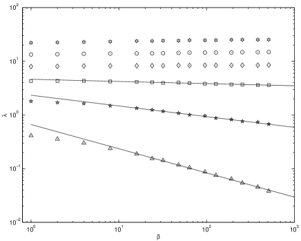
FIG. 2.: The six eigenvalues $\langle\lambda_{i}\rangle_{\beta}$ of the moment of inertia tensor $T$ are plotted against $\beta$ in a log-log scale for $D=6$ and $N=3$. The straight lines for the smallest three eigenvalues represent the fits to the power law behavior.

Discussion.—

The results presented in the previous section shows clearly that the stationarity of the phase $\Gamma^{(i)}$ indeed enhances lower-dimensional brane configurations considerably, thus demonstrating our mechanism. In particular, while the existence of saddle-point configurations other than the configurations in $\Omega_{D-2}$ is not excluded, our results suggest that such configurations, even if they exist, can safely be neglected on statistical grounds. Given this observation, the reason why we obtain the dimensionality ‘three’ from the dominant saddle-point configurations of the simplified model (6) can be understood analytically. As has been done in Ref. [7] for the IIB matrix model, we can rewrite the $\beta\rightarrow\infty$ limit of the simplified model (6) as an integral over the configurations in $\Omega_{D-2}$. The gaussian fluctuation of the phase $\Gamma^{(\rm i)}$ should be taken into account by the corresponding Hesse matrix, which is, in the present case, just the square of the one for the IIB matrix model (or its $D=6$ version). Due to this, the gaussian fluctuation enhances lower-dimensional brane configurations even more strongly than in the IIB matrix model and overwhelms the entropical barrier against having those configurations.

The fact that the lowering of the dimensionality stops at three instead of continuing further down can be understood as follows. We first note that the fermion integral $Z_{f}[A]$ vanishes for configurations in $\Omega_{2}$ [7]. Therefore, the phase $\Gamma^{(i)}$ is actually ill-defined for configurations in $\Omega_{2}$. Still, we can consider configurations with $A_{1}$, $A_{2}$ being generic and $A_{i}~{}(i=3,\cdots,D)$ being of order $\epsilon$. One can easily see that the function $F[A]$ is diverging as $\epsilon^{-2}$ for $\epsilon\rightarrow 0$. Therefore, the $\beta$ term in (6) suppresses configurations in $\Omega_{2}$ strongly. (In other words, configurations in $\Omega_{2}$ are not saddle-point configurations, although $\Omega_{2}\subset\Omega_{D-2}$.)

As is clearly shown in the present work, the enhancement occurs precisely when the space-time becomes a flat lower-dimensional hyperplane, which we consider as a very attractive feature of our mechanism. Namely, our mechanism has a built-in structure in which the brane that appears as a result of the nonperturbative string dynamics is very likely to be flat. According to our mechanism, scenarios with two separated branes (i.e. our world and the so-called ‘Planck’ brane as in Ref. [4]), their extensions to many branes [15], and scenarios with mutually intersecting branes [16] seem to be unnatural.

Let us also comment on a connection of our mechanism to the brane world scenario. In Ref. [17], the IIB matrix model is expanded around a D3-brane configuration perturbatively and four-dimensional noncommutative Yang-Mills theory has been obtained [18]. The (perturbatively stable) theory, which is obtained in this way from the IIB matrix model, has been recently identified [20] with a type IIB superstring theory in $\mbox{AdS}_{5}\times\mbox{S}^{5}$ with an infinite $B$-field background. Remarkably the metric that appears in the corresponding supergravity solution takes the form of Randall-Sundrum’s type [6], and thereby allows for a four-dimensional Newton’s law. We expect that brane configurations similar to the D3-brane configuration considered above as a background in the IIB matrix model should appear dynamically as a result of our mechanism. Thus our mechanism is rather directly related to the brane world scenario.

In the IIB matrix model, the enhancement and the entropical barrier are exactly balanced and the actual dimensionality of the brane is expected to be determined as a result of large $N$ dynamics. In this regard, we recall that the low-energy effective theory of the IIB matrix model has been shown to be described by a branched-polymer like system in Ref. [21]. There it was further argued that a typical double-tree structure that appears in the effective theory might cause a collapse of the configuration to a lower-dimensional manifold. Whether the actual dimensionality of the brane turns out to be four or not can be investigated directly by performing the integration over the saddle-point configurations as formulated in Ref. [7]. We hope that Monte Carlo techniques developed in Ref. [10] will enable us to address such an issue in near future.

REFERENCES

- [1] Electronic mail: nisimura@nbi.dk. Permanent address: Department of Physics, Nagoya University, Nagoya 464-8602, Japan.
- [2] Electronic mail: vernizzi@nbi.dk.
- [3] N. Arkani-Hamed, S. Dimopoulos and G. Dvali, Phys. Lett. B 429, 263 (1998); I. Antoniadis, N. Arkani-Hamed, S. Dimopoulos and G. Dvali, Phys. Lett. B 436 257 (1998).
- [4] L. Randall and R. Sundrum, Phys. Rev. Lett. 83, 3370 (1999) .
- [5] V.A. Rubakov and M.E. Shaposhnikov, Phys. Lett. B 125, 139 (1983); E. Verlinde and H. Verlinde, J. High Energy Phys. 0005, 034 (2000); C. Schmidhuber, hep-th/9912156, hep-th/0005248.
- [6] L. Randall and R. Sundrum, Phys. Rev. Lett. 83, 4690 (1999).
- [7] J. Nishimura and G. Vernizzi, J. High Energy Phys. 0004, 015 (2000).
- [8] N. Ishibashi, H. Kawai, Y. Kitazawa and A. Tsuchiya, Nucl. Phys. B 498, 467 (1997).
- [9] T. Banks, W. Fischler, S.H. Shenker and L. Susskind, Phys. Rev. D 55, 5112 (1997).
- [10] J. Ambjørn, K.N. Anagnostopoulos, W. Bietenholz, T. Hotta and J. Nishimura, J. High Energy Phys. 0007, 011 (2000).
- [11] The same conclusion has been obtained analytically for a ‘quenched’ model, which is defined by omitting the pfaffian completely [12].
- [12] T. Hotta, J. Nishimura and A. Tsuchiya, Nucl. Phys. B 545, 543 (1999).
- [13] In the case, the fermion integral is proved to be real positive for arbitrary , which allows a standard Monte Carlo study of the large dynamics [14].
- [14] J. Ambjørn, K.N. Anagnostopoulos, W. Bietenholz, T. Hotta and J. Nishimura, J. High Energy Phys. 0007, 013 (2000).
- [15] I. Oda, Phys. Lett. B480, 305 (2000); H. Hatanaka, M. Sakamoto, M. Tachibana and K. Takenaga, Prog. Theor. Phys. 102, 1213 (1999).
- [16] N. Arkani-Hamed, S. Dimopoulos, G. Dvali and N. Kaloper, Phys. Rev. Lett. 84, 586 (2000).
- [17] H. Aoki, N. Ishibashi, S. Iso, H. Kawai, Y. Kitazawa and T. Tada, Nucl. Phys. B 565, 176 (2000).
- [18] This equivalence has been understood at a fully nonperturbative level as a Morita equivalence of noncommutative gauge theories [19].
- [19] J. Ambjørn, Y.M. Makeenko, J. Nishimura and R.J. Szabo, J. High Energy Phys. 9911, (1999) 029; Phys. Lett. B 480, 399 (2000); J. High Energy Phys. 0005, 023 (2000).
- [20] N. Ishibashi, S. Iso, H. Kawai and Y. Kitazawa, hep-th/0004038.
- [21] H. Aoki, S. Iso, H. Kawai, Y. Kitazawa and T. Tada, Prog. Theor. Phys. 99, 713 (1998).