NYU-TH-00/06/01

OUTP-00-26P

TPI-MINN-31/00

UMN-TH-1910

hep-th/0006213

Topological Effects in Our Brane World From Extra Dimensions

G. Dvali
Department of Physics, New York University, New York, NY 10003, USA
Ian I. Kogan
Theoretical Physics, Oxford University, 1 Keble Road, Oxford OX13NP, UK
and
M. Shifman
Theoretical Physics Institute, University of Minnesota, Minneapolis, MN 55455, USA

Abstract

The theories in which our world presents a domain wall (brane) embedded in large extra dimensions predict new types of topological defects. These defects arise due to the fact that the brane on which we live spontaneously breaks isometries of the extra space giving mass to some graviphotons. In many cases the corresponding vacuum manifold has nontrivial homotopies – this gives rise to topologically stable defects in four dimensions, such as cosmic strings and monopoles that carry gravimagnetic flux. The core structure of these defects is somewhat peculiar. Due to the fact that the translation invariance in the extra direction(s) is restored in their core, they act as “windows” to the extra dimensions. We also discuss the corresponding analog of the Alice strings. Encircling such an object one would get transported onto a parallel brane.

1 Introduction.

In the conventional Kaluza-Klein approach [1] the Universe has a topology $M_{4}\otimes K$, where $M_{4}$ is our four-dimensional Minkowski space and $K$ is some compact manifold, with the volume typically set by a fundamental Planck length $l_{\rm P_{f}}=1/M_{\rm P_{f}}$. Isometries of $K$ are then seen as gauge symmetries of an effective four-dimensional theory, with the role of the gauge fields played by extra components of the graviton (the so-called graviphotons). In the theories where our world is a domain wall (brane) embedded in the extradimensional space [2, 3] the situation drastically changes. First, the domain wall allows one [4] to choose a much larger size of the extra dimensions, $R\gg l_{\rm P_{f}}$. Second, since the branes are localized in $K$, they spontaneously break all or a part of the isometries of $K$; the corresponding graviphotons get masses. In our four-dimensional world this breaking is seen as a Higgs effect, where the role of the Goldstones eaten up in the Higgs mechanism is played by the zero modes of the broken translational invariance [5, 6].

(In addition in the presence of branes and gravity, the space-time is not a direct product $M_{4}\otimes K$ strictly speaking, due to the gravitational field of the brane. However, at least for the spaces with the co-dimension $N\geq 2$, this effect is of little importance for the present purposes, and can be ignored. An example of a solution including gravity which describes a single brane on $M_{4}\otimes S_{1}$ is given in [7].)

The purpose of the present work is to study possible macroscopic topological consequences of the above picture for four-dimensional physics. Our starting point is the following four observations on which we would like to elaborate.

$\bullet$ If topology of $K$ is nontrivial and so is that of the target space ${\cal T}$ (i.e. the space of fundamental fields), there emerge topologically nontrivial mappings $K\to{\cal T}$ which are characterized by various moduli. The moduli become dynamical fields of the low-energy four-dimensional theory.

$\bullet$ The number of the moduli is equal to or larger than the number of the symmetries of the theory broken by the mapping under consideration. If the topological number of the mapping $K\to{\cal T}$ is larger than one, this gives rise to “parallel” branes and the “horizontal” proliferation of the low-energy four-dimensional fields (multiple generations). Even for the unit topological number of the mapping $K\to{\cal T}$, the number of the moduli may be significantly larger than the number of the broken isometries. This phenomenon corresponds to dynamical symmetries and their Goldstones.

$\bullet$ Topology of the moduli space is typically nontrivial too. In other words, the space of the effective low-energy four-dimensional fields is topologically nontrivial. This generates physically observable topological defects in our world.

$\bullet$ Inclusion of gravity and its interplay with nontrivial topology leads to peculiar effects.

In this work we will focus on those moduli that correspond to the spontaneously broken isometries of $K$. Let $G$ be an isometry group of $K$. A given domain wall breaks this group down to a subgroup $H$. Then $G/H$ defines a vacuum manifold; if homotopies of this manifold are nontrivial, the theory admits topologically nontrivial stable configurations. This structure has a simple geometric meaning, as seen directly from the high-dimensional Universe. Assume, for definiteness, that the brane at hand is a three-brane. Then it is a point on $K$. The space of all possible locations of the brane is $K$ itself. Now imagine that $\pi_{n}(K)\neq 0$. In other words, $K$ contains $n$-dimensional closed surfaces that can not be contracted to a point in $K$.

For $n=1$ and 2, such surfaces can be mapped on the spatial boundary of our $M_{4}$. Such configurations will be topologically nontrivial; they can not be deformed to a trivial vacuum continuously. They correspond to a constant change of the position of the brane on $K$ as we travel around a closed surface in 3+1 dimensions. For instance, at $n=1$ the configuration we will deal with is a cosmic string. Winding around such a string, the four-dimensional observer will make a full circle on $K$ along the extra dimension.

An intriguing question is what is the core structure of such defects? Usually the broken symmetries get restored (at least, partially) in the core of the topological defects. The symmetries in question are the translations in the extra space. Their restoration would mean that there is a “hole” in the domain wall – in a sense, the topological defects open a door in the extra space and can link together “parallel” brane worlds.

The organization of the paper is as follows. In Sec. 2 we discuss strings, Sec. 3 is devoted to monopoles, Sec. 4 deals with the Alice strings, in Sec. 5 we briefly discuss proliferation of moduli (some of them may be related to dynamical rather than geometrical symmetries). Finally, the graviphoton mass is considered in Appendix.

2 The Kaluza-Klein Cosmic String

In this section we consider the simplest defect of the type discussed above, the Kaluza-Klein cosmic string. Although this structure has nothing to do with the classical Kaluza-Klein set-up [1] – it exists only in the theories with the branes – we keep the name “ Kaluza-Klein,” since this string carries a magnetic flux of the graviphoton field. The magnetic flux connects the Kaluza-Klein monopoles.

The simplest possibility with nontrivial $\pi_{1}$ is to assume that $K=S_{1}$. This has the isometry group $G=U(1)$, broken by the brane down to identity. The brane position on $S_{1}$ is parametrized by one scalar modulus $y$. This position can slowly vary with $x_{\mu}$, the four-dimensional space-time point. Thus, the four-dimensional observer will perceive $y(x_{\mu})$ as a low-energy scalar field on $M_{4}$. The target space of $y$ is obviously a circle $S_{1}$. The corresponding fundamental group $\pi_{1}(S_{1})=Z$.

We will be interested in the configurations in which the brane sweeps a full circle around $K=S_{1}$ as we travel along a four-dimensional closed path at infinity. Let $0\leq y<L$ (the points $0$ and $L$ are identified), $t$ is time of $M_{4}$, while $r,\theta$ and $z$ are the spatial coordinates on $M_{4}$ ($r$ and $\theta$ are the polar coordinates). The Kaluza-Klein cosmic string oriented along the $z$ axis then corresponds to the following asymptotic configuration

$$\theta={2\pi ny\over L}$$ (1)

where $n$ is an integer, the winding number.

In the absence of gravity, such configuration has a logarithmically divergent energy at large $r$. This divergence comes from the long-range gradient energy of the Goldstone field living on the brane. At distances $\gg L$ the only relevant degree of freedom describing the brane dynamics is the Goldstone mode $\chi\equiv\sqrt{T}\,y(x_{\mu})$ of the broken translational invariance. Here $T$ is the brane tension (energy per unit three-surface). The low-energy Lagrangian obviously has the form (modulo higher derivatives)

$${\cal L}_{\rm eff}=T\,(\partial_{\mu}y(x))(\partial^{\mu}y(x))\,.$$ (2)

It is clear that the configuration (1) corresponds to the winding of the Goldstone field and results in the logarithmically divergent energy per unit length of the string,

$$E\sim L^{2}\,T\,n\,{\log}\rho\,,$$ (3)

where $\rho$ is the maximal distance in the direction perpendicular to the $z$ axis along which the string is aligned, and $L$ is the size of the fifth dimension. Such logarithmically divergent energy is typical for global cosmic strings. In the case at hand it simply indicates that in the absence of gravity the Kaluza-Klein cosmic strings would be global [10].

However, in actuality this divergence is compensated by the graviphoton field, which takes a pure gauge form at infinity,

$$A_{\theta}={n\over g}\,,$$ (4)

where $g=1/(M_{\rm P_{f}}L)$ is an effective gauge coupling. The topological defect we deal with here is of the type of a local Abrikosov-Nielsen-Olesen string [11].

We pause here to make an important remark. In the topologically trivial sector the graviphoton gets mass through the Higgs mechanism – the spontaneous breaking of U(1). Say, if the original space is five-dimensional, the graviphoton mass squared is proportional to the brane tension and inversely proportional to the four-dimensional Planck mass $M_{p}^{2}=M_{\rm P_{f}}^{3}\,L$, (details are given in Appendix)

$$M^{2}_{V}=\frac{T}{M_{p}^{2}}\,.$$ (5)

Analogous formulae can be obtained for general p-branes in the D-dimensional space-time. Although the above conclusion has been reached in an effective field theory, it is quite general and must be applicable to D-branes in string theory too – in the presence of D-branes graviphotons will become massive. In the weak coupling limit the D-brane tension is very large, it grows as $T\sim M_{\rm str}^{4}/g_{\rm str}\,$ and, at the same time, the Planck mass scales as $M_{p}^{2}\sim M_{\rm str}^{2}/g_{\rm str}^{2}\,$. Assembling these factors we obtain that the graviphoton mass scales as

$$M^{2}_{V}\sim g_{\rm str}M_{\rm str}^{2}\,.$$ (6)

The fact that this mass is proportional to $g_{\rm str}$, rather than to $g_{\rm str}^{2}$, is a pure D-brane effect; it is due to the fact that the Born-Infeld action describing the D-brane dynamics is proportional to $1/g_{\rm str}$.

Returning to the field configuration (1), (4), we observe that the magnetic flux is trapped in the core of the Kaluza-Klein string. Therefore, such strings must be able to end on the Kaluza-Klein monopoles. This leads us to the conclusion that in the brane scenarios the Kaluza-Klein monopoles are not stable; rather, they get connected by the Kaluza-Klein cosmic strings and annihilate.

Infinite isolated cosmic strings can also exist. At large distances the behavior of the Kaluza-Klein cosmic strings is similar to the conventional gauge strings in U(1) theories. The core structure of these objects is somewhat peculiar, however.

Normally the order parameter responsible for the symmetry breaking must vanish in the core where the U(1) symmetry gets restored. However, in the case at hand the order parameter is the position of the brane on $K=S_{1}$. Thus, we expect a “hole” in the brane at the location of the defect. This hole is a domain on $M_{4}$ where the translational invariance on $K$ is restored. In the case at hand this is the $z$ axis. This domain acts as a “window” in the extra dimensions.

In the case when the brane is a topological soliton of the type considered in Ref. [8] the nature of the hole is easy to visualize. Let us discuss, for instance, the theory of one fundamental field $\Phi$, with a non-simply connected target space. One can consider, for instance, a real scalar field $\Phi$ defined modulo $2\pi$ on $M_{4}\otimes S_{1}$. Assume that the potential is

$$V=\frac{1}{2}\left(\frac{C}{1+\beta\cos\Phi}\right)^{2}\,,\qquad C=\frac{2\pi}{L}\,,$$ (7)

and the constant $\beta$ is positive and slightly less than 1. This theory admits a stable soliton solution defined by the equation

$$\frac{2\pi}{L}\left(y-y_{0}+\frac{L}{2}\right)=\Phi+\beta\sin\Phi\,.$$ (8)

Here $y_{0}$ is the soliton center. The solution $\Phi(y)$ interpolates between $\Phi=0$ and $\Phi=2\pi$ as $y-y_{0}$ varies from $-L/2$ to $+L/2$. By choosing the parameter $\beta$ sufficiently close to 1, one regulates the width of the brane in the $y$ direction making it as small as it is desired. Since $\Phi$ is periodic such solitons are perfectly compatible with compactness of $K$.

Now let us make $y_{0}$ a slowly varying function of $x_{\mu}$. The cosmic string lying along the $z$ axis is formed if $y_{0}$ changes from 0 to $L$ as we wind around the $z$ axis in the perpendicular plane. If we are sufficiently far from the $z$ axis the brane soliton has the form following from Eq. (8). However, at $r\to 0$ the location of the brane on the circle $K$ is ill-defined. This means that at $r\to 0$ the fundamental field configuration continuously evolves from (8) to

$$\frac{2\pi}{L}\left(y-y_{0}+\frac{L}{2}\right)=\Phi\,.$$ (9)

The latter corresponds to the brane completely smeared over $K$, so that $y_{0}$ looses its meaning of the brane center. The width of the brane in the $K$ direction becomes $L$. The field configuration (9) has an excess of potential energy – this is standard for the core of the string. An observer approaching the cosmic string will leave our brane and fill $K$ entirely.

The whole construction can be viewed as a circular “staircase” – split our three-dimensional space in a sequence of two-dimensional planes attached to the given string; passing from one plane to another we simultaneously shift in the fifth direction, as shown in Fig. 1. In fact, the picture is somewhat more contrived, since the slices $y=0$ and $y=2\pi R\equiv L$ must be identified, but this is impossible to show in the figure.

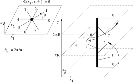
Figure 1: $K=$U(1) Kaluza-Klein string as a “staircase.” Our three-dimensional space is represented as an ensemble of planes attached to the string which lies along the $z$ axis (see a slice on the left). As we move from one plane to another we simultaneously shift in the fifth direction. A full winding corresponds to the shift from $y=0$ to $y=2\pi R\equiv L$.

If originally there were several branes on $K$ (this would correspond to higher windings of $\Phi(y)$) at $r\to 0$ the proper field configuration must evolve to

$$\frac{2\pi\nu}{L}\left(y-y_{0}+\frac{L}{2}\right)=\Phi\,,$$ (10)

where $\nu$ is the winding number. Near the position of the cosmic string all $\nu$ branes fuse together. The construction with several “parallel” branes may be promising from a phenomenological standpoint [9].

3 The Monopoles

Let us now pass to the discussion of nontrivial $\pi_{2}(K)$. We will show that the brane can create certain topologically stable configurations which look as monopoles in four dimensions. Again, we will focus on the simplest manifold with nontrivial $\pi_{2}$, the two-sphere $K=S_{2}$. The brane breaks the isometries of $K$. The symmetry breaking pattern on $K$ is SU(2) $\to$ U(1). Correspondingly, the position of the brane on $S_{2}$ can be characterized by two angular coordinates $0<\theta_{K}<\pi$ and $0<\phi_{K}<2\pi$. In the low-energy four-dimensional theory $\theta_{K}(x_{\mu})$ and $\phi_{K}(x_{\mu})$ become the Goldstone fields. To parametrize $M_{4}$, instead of $t,r,\theta,z$ of Sec. 2 we now introduce the spherical coordinates $r,\theta,\phi$. Since the brane can fluctuate and move on $S_{2}$, the angles $\theta_{K}$ and $\phi_{K}$ are slowly varying functions of $r,\theta,\phi$ and our Minkowski time $t$. The topologically stable monopole configuration is given by the following mapping:

$$\theta_{K}=\theta,~{}~{}~{}{\rm and}~{}~{}~{}\phi_{K}=\phi\,,$$ (11)

at $r$ sufficiently far from the monopole core, plus the appropriate configuration of the graviphoton fields. The general structure is the same as that of the ’t Hooft-Polyakov monopoles [12] in the Georgi-Glasow model. This configuration carries a topological charge since it corresponds to the mapping $(S_{2})_{K}\rightarrow(S_{2})_{M_{4}}$, where the second sphere is the spatial boundary of the spatial part of $M_{4}$.

At $r$ approaching zero the symmetry must be restored, and the “former” brane must delocalize on $K$ much in the same way as in the cosmic string example (Sec. 2). Thus, the core of the monopole presents an exit into $K=S_{2}$. If there are several “parallel” branes, the monopole core will connect all of them. In a sense, this is even a more interesting object than the string of Sec. 2 since it is fully localized on $M_{4}$. The mass of such monopole is expected to be of order

$$M_{\rm monopole}\sim(\sqrt{T}R^{2})\,M_{\rm P_{f}}\,,$$ (12)

where $R$ is the radius of $S_{2}$. The monopole mass can be much lighter than the fundamental Planck scale, since in our scenario the product $\sqrt{T}R^{2}$ depends on dynamical details of the underlying theory, and can well be small. Finding this monopole would be an exciting endeavor since one could channel signals to/from other branes through its core.

4 The Alice Strings from the Branes

In this section we will deal with $K=S_{2}$, but nontrivial $\pi_{1}$, rather than $\pi_{2}$.

In the example of Sec. 3, the brane was represented by a point on $K=S_{2}$. What happens if the brane is represented by two or more rigidly connected points? For instance, assume the brane to be described by two identical points in the opposite poles of the two-sphere. After one of the isometries of $S_{2}$ is broken, the surviving symmetry then is $U(1)\times Z_{2}$, since one can interchange the poles without affecting the expectation value of the brane position moduli on $K$. Strictly speaking, the surviving symmetry is not the direct product, however, since $Z_{2}$ flips the sign of the $U(1)$ generator. This sign-flipping results in the existence of Alice strings [13] in the four-dimensional space $M_{4}$.

To see that this is indeed the case, let the surviving U(1) generator be $\tau_{3}$ (the third Pauli matrix). Then $Z_{2}$ can be represented as

$$U_{Z_{2}}=\exp\{-(i/2)\,\pi\,\tau_{2}\}\,,$$

so that $U_{Z_{2}}^{-1}\,\tau_{3}U_{Z_{2}}=-\tau_{3}$. The vacuum manifold contains unshrinkable paths which start at identity and end at $U_{Z_{2}}$. This can be parametrized by a group transformation

$$U_{\vartheta}=\exp\{-(i/2)\,\vartheta\,\tau_{2}\}\,,\quad\vartheta\in[0,\pi]\,.$$ (13)

The Alice string configuration is obtained by identifying $\vartheta$ with the angle $\theta/2$ in $M_{4}$ introduced in Sec. 2. In other words, as one winds once around the $z$ axis in $M_{4}$ (far away from the axis) the position moduli on $K$ drift from the north to the south pole (which are identified). This configuration is obviously topologically stable.

In this way the opposite points on $K$ interchange places when one travels once around the string (far away from the string axis). If such observer completes his/her journey and comes back to the point of departure, he/she will find U(1) charges to be conjugated. Indeed, assume the travel was adiabatic. The wave function of any state will track observer’s position so that the wave function will acquire the gauge factor

$$\psi(\theta)=\left(U_{\vartheta}\right)^{q}\psi(0)\,,$$ (14)

where $q$ is the U(1) charge of the state under consideration measured in the units of the fundamental charge. One can measure the U(1) charge at the beginning and the end of the journey by acting by $\tau_{3}$ on states $|\psi(0)\rangle$ and $|\psi(2\pi)\rangle$, respectively, assuming the travel to be adiabatic. However,

$$|\psi(\theta=2\pi)\rangle=\left(U_{Z_{2}}\right)^{q}\,|\psi(0)\rangle\,.$$

For all odd $q$

$$\tau_{3}|\psi(\theta=2\pi)\rangle=(-1)\,|\psi(\theta=2\pi)\rangle\,,$$

while for even $q$

$$\tau_{3}|\psi(\theta=2\pi)\rangle=(+1)\,|\psi(\theta=0)\rangle\,.$$

For instance, if we transport a fermion in the fundamental representation of the original SU(2) around the string, its U(1) charge will flip the sign. This is a typical behavior for the Alice strings.

In the present case the emerging Alice string has a clear-cut geometric interpretation. The conserved U(1) is nothing but the rotation of $S_{2}$ around the axis connecting the north and south poles. Traveling around the string (i.e. winding around the $z$ axis in $M_{4}$) interchanges the north/south poles and thus, the angular momentum of any state. One can visualize this as a loop made of a Möbius strip.

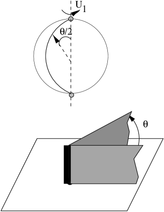
Figure 2: $S^{2}$ with two branes at antipodal points. The Alice string is given by the large semicircle connecting these two points. The (3+1)-dimensional space is distributed all over the semicircle in such a way that a plane attached to the Alice string at angle $\theta$ is connected to the point on the semicircle parametrized by the angle $\vartheta=\theta/2$. Making a full $2\pi$ rotation of the plane we one moves from the north to the south pole on $S^{2}$ and by this changes the sign of the U(1) generator.

In a similar manner one can get strings which interchange two gauge groups (or possibly more than two). Let us consider, for example, the case when the original gauge symmetry $G$ (related to the isometries of $K$) is broken down to a subgroup $H\times H$. We want to have a $Z_{2}$ subgroup of $G$ which does not commute with $H\times H$ in order to generate a $Z_{2}$ string such that after making a full turn we exchange two $H$’s. This will have a very spectacular effect – if such a string passes between a source and a detector measuring the flux of charged particles (charged with respect to one of the gauge groups only), the detector will see only a half of the beam. The reason that half of the particles will be transformed into particles charged with respect to a second group and our detector will not see them. What half will undergo the transition depends on the history of how the detector and the source were prepared.

How to make such a string? Take the manifold $G/(H\times H)$. By definition there is a point $A$ on this manifold which is stable under $H\times H$ – so if we put a brane at this point the $H\times H$ subgroup of $G$ remains unbroken. Consider $G$ as an ensemble of $2n\times 2n$ matrices and $H$ as $n\times n$. Take now the group element

$$T=\left(\begin{array}[]{cc}0&I\\ I&0\\ \end{array}\right)$$ (17)

where $I$ is the $n\times n$ identity matrix. One can see that $T^{2}=1$ while $T$ interchanges two $H$ subgroups. The antipodal point $B$ is constructed by acting by $e^{i\pi T}$ on $A$. We then consider the coset $G/(H\times H)$ with the branes placed at both points $A$ and $B$. Besides the unbroken symmetry $H\times H$ the group $Z_{2}$ is also unbroken – it interchanges $A$ and $B$ (with one brane this symmetry would be broken). Moreover, this $Z_{2}$ does not commute with $H\times H$. The Alice string is obtained by splitting our space in planes and attaching them along the line $e^{i\theta T/2}A$ for $\theta$ between $0$ and $2\pi$. In principle, one may try to consider $Z_{N}$ strings by invoking $H\times..\times H$ symmetry with $N$ copies of $H$ and the coset $G/(H\times..\times H)$.

(Let us parenthetically note that there may occur obstructions to construction of the Alice strings, see e.g. [14]. Classification of all possible Alice strings within the brane scenarios is an interesting question.)

5 Proliferation of Moduli

The effective theories considered so far were those of the geometric moduli related to the isometries of $K$. The number of moduli can be much larger, however, since in the given fundamental theory responsible for the brane formation symmetries may be dynamical. The nontrivial topology of the moduli space can be much more contrived than that of $K$. Here we will discuss a simple example of this phenomenon.

Assume that $K=S_{2}$ and the underlying theory is the nonlinear O(3) sigma-model, with the fundamental field $\vec{n}$ where $\vec{n}^{2}=1$. The combined action, including gravity, is

$$S=M_{\rm P_{f}}^{4}\int d^{4}xd^{2}y\sqrt{G}R^{(6)}+\int d^{4}xd^{2}y\sqrt{G}\left[\frac{1}{2}G^{MN}\partial_{M}\vec{n}\partial_{N}\vec{n}\right]+...$$ (18)

where $M_{\rm P_{f}}$ and $R^{(6)}$ are the six-dimensional fundamental Planck mass and the scalar curvature, respectively, the dots stand for the possible fermion terms if the theory is supersymmetric, and finally $M,N=0,1,2,3,4,5$.

Now we consider classical solutions of the equations of motions with nontrivial topology, depending on $x_{4}$ and $x_{5}$ where $x_{4,5}$ parametrize $S_{2}$. These are nothing but the Polyakov-Belavin instantons [15].

Using the standard stereographic projection

$$W=\frac{n_{1}+in_{2}}{1+n_{3}}$$ (19)

one can introduce a complex field $W$ depending on a complex variable $z$ ($S_{2}$ is the Kähler manifold allowing for the complex structure)

$$W(z)=\prod_{i=1}^{K}\frac{z-b_{i}}{z-a_{i}}$$ (20)

where $z$ is the complex coordinate on $CP^{1}$, and $K$ is the winding number. Moreover, $b_{i}$ and $a_{i}$ are complex numbers, $2K$ altogether, representing the moduli parameters of the soliton.

Now we can make them coordinate-dependent,

$$W(z,x^{\mu})=\prod_{i=1}^{K}\frac{z-b_{i}(x)}{z-a_{i}(x)}\,.$$ (21)

The action can be written as (note that $\partial_{z}\bar{W}=0$)

$$\int d^{4}x\frac{dzd\bar{z}}{(1+|z|^{2})^{2}}\sqrt{g}\left[\frac{|\partial_{z}W|^{2}}{(1+|W|^{2})^{2}}+G^{\mu\nu}\frac{\partial_{\mu}W\partial_{\nu}\bar{W}}{(1+|W|^{2})^{2}}+G^{\mu z}\frac{\partial_{z}W\partial_{\mu}\bar{W}}{(1+|W|^{2})^{2}}+\mbox{ c.c.}\right].$$ (22)

We see that

$$\partial_{z}W=W\sum_{i=1}^{K}\left[\frac{1}{z-b_{i}}-\frac{1}{z-a_{i}}\right]\,,$$

$$\partial_{\mu}W=W\sum_{i=1}^{K}\left[\frac{\partial_{\mu}a_{i}}{z-a_{i}}-\frac{\partial_{\mu}b_{i}}{z-b_{i}}\right].$$ (23)

Substituting this in the action we get an effective Lagrangian describing dynamics of the collective coordinates (moduli) $a_{i}(x)$ and $b_{i}(x)$,

$$S[a,b] = \int d^{4}x\sqrt{g}G^{\mu\nu}\left[F^{ij}(a,b)\partial_{\mu}a_{i}\partial_{\nu}\bar{a}_{j}\right.$$ (24)

$$+ \left.B^{ij}(a,b)(\partial_{\mu}a_{i}\partial_{\nu}\bar{b}_{j}+\partial_{\mu}b_{i}\partial_{\nu}\bar{a}_{j})+H^{ij}(a,b)\partial_{\mu}b_{i}\partial_{\nu}\bar{b}_{j}\right]\,,$$

where $F^{ij},B^{ij},H^{ij}$ represent a metric on the $2K$-dimensional moduli space. We do not know the explicit form of the metric on the multi-instanton moduli space (i.e. at $K>1$). It is known, however, that this moduli space is a Kähler manifold.

In case of $S_{2}$ we have three graviphotons – the gauge symmetry is SU(2) – but we have an arbitrary number of the Goldstone modes provided $K$ can be chosen at will. If $K=1$, the Goldstone action for the moduli $a$ and $b$ can be easily found. We can introduce two new collective coordinates: $X=a-b$ (the size of the instanton and U(1) orientation) and $Y=(a+b)/2$ (the position of the center).

We will work in the approximation when $a$ and $b$ are small in which case we explore only a small patch on $S_{2}$ which is an open region of the plane. The action of the SU(2) generators in this limit is nothing but a U(1) rotation (which will be our unbroken symmetry) and two translations (the non-Abelian nature of the SU(2) is not seen in this approximation).

The action (24) in this case can be written as a sum of two independent actions, for the $X$ field

$$S_{X}\sim\int d^{4}x\ln|X|^{2}|\partial_{\mu}X|^{2}\,,$$ (25)

and for the $Y$ field

$$S_{Y}\sim\int d^{4}x|\partial_{\mu}Y|^{2}\,.$$ (26)

After the inclusion of the graviphotons the action for the $Y$ fields becomes

$$(\partial_{\mu}Y+A_{\mu}^{+})(\partial^{\mu}\bar{Y}+A^{\mu-})\,.$$

We arrive at the Georgi-Glashow model SU(2) $\rightarrow$ U(1). Let us note that the modulus $X$ does not mix with the graviphoton, only $Y$ does. This is because it is $Y$ that is transformed by two broken symmetries of SU(2).

For $K>1$ we have more massless particles. In the supersymmetric case we have not only bosonic zero modes, but fermionic as well. The latter are chiral, so we can create several generations of the chiral matter. This example shows that having a topological defect within a brane world scenario may not only open a window to extra dimensions but can also create a large number of light fields. To this end, the topological defect at hand must have a large enough topological charge, i.e. a large dimension of its moduli space.

6 Conclusions

In the theories where our world is trapped on the brane(s) embedded in large compact extra dimensions the Kaluza-Klein scenarios get drastically modified. Since the brane break isometries of the extra space $K$, the graviphotons become massive via an analog of the Higgs mechanism. In addition, a nontrivial topology of the compact space $K$ gets entangled with the topology of our world, giving rise to strings (in case of nontrivial $\pi_{1}$) and monopoles (nontrivial $\pi_{2}$) of a special geometric nature (we call them Kaluza-Klein defects, although they can appear only in the presence of branes). In the core of the Kaluza-Klein defects the full symmetry of $K$ gets restored, so that their cores represent a natural channel of exit into $K$. If there are several “parallel” branes, they may get connected through the core of the monopole or the axis of the strings. We have considered two types of strings – the Abrikosov-Nielsen-Olesen string and the Alice string.

A large number of additional moduli may (and usually do) naturally emerge, which have a dynamical rather than geometric origin. This results in the proliferation of matter trapped on the branes. The number of moduli is proportional to the topological number of the mapping which need not necessarily be unity. The topology of the moduli space is typically more contrived than that of $K$. Implications of this observation for the topological defects observable in our world are yet to be studied.

The original motivation [2] for introducing brane worlds was the desire to localize matter in a “ transverse” space of a small volume embedded in a noncompact space of the infinite volume. The latter was then replaced by a compact space of a large size [4, 5], where the branes were supposed to accomplish the same mission of localization. At present the importance of this aspect of the brane scenarios – localization – fades away, as, on the one hand, people start to realize that other aspects of the brane scenarios may be potentially instrumental, and on the other hand, extra spaces of exceedingly smaller sizes are emerging in various theories (e.g. [16]). Other goals which might be achieved in the brane world scenarios are taking over; they are: (i) supersymmetry breaking and separation of chiralities (i.e. making our matter chiral starting from a nonchiral set) [3]; (ii) hierarchies in the SUSY breaking parameters and mass parameters [9]; (iii) generation of a mass term for the graviphotons [5, 6]; (iv) proliferation of matter – i.e. the “parallel” matter generations. The topological defects of the special type, discussed in this paper, is one more new aspect.

Acknowledgments

We are grateful to A. Tseytlin for a useful discussion and to Albert Schwarz for useful communications. The work of G.D. was supported in part by David and Lucille Packard Foundation Fellowship for Science and Engineering. The work of M.S. was supported by DOE grant DE-FG02-94ER408. The work of I.K. was supported in part by PPARC rolling grant PPA/G/O/1998/00567 and the EC TMR grant FMRX-CT-96-0090

Appendix: Branes Make Graviphotons Massive

The brane-Higgs effect has been already discussed in [5, 6]. Here we present it for completeness and also give a detailed derivation of the graviphoton mass. Let us start from the simplest situation: consider a domain wall in the five-dimensional space $M^{4}\times S_{1}$ with four noncompact coordinates $x_{0},x_{1},x_{2},x_{3}$ and one compact (fifth) coordinate $x_{4}=y$. Imagine that the domain wall is made of a scalar field $\Phi$; the combined action including gravity is

$$S=M_{\rm P_{f}}^{3}\int d^{4}xdy\sqrt{G}R^{(5)}+\int d^{4}xdy\sqrt{G}\left[\frac{1}{2}G^{MN}\partial_{M}\Phi\partial_{N}\Phi+V(\Phi)\right]$$ (A.1)

where $M_{\rm P_{f}}$ and $R^{(5)}$ are the five-dimensional Planck mass and the scalar curvature, respectively, and $M,N=0,1,2,3,4$. The Greek letters $\mu,\nu=0,1,2,3$ are reserved for the four-dimensional indices. The signature is $(-,+,+,+,+)$. The explicit form of the potential $V(\Phi)$ is not important here – the only thing we have to know is that the target space has a nontrivial topology and there are topologically stable classical solutions. For example one can consider the potential (7). Let us forget about gravity for a moment. The domain wall $\Phi_{0}(y)$ in the fifth direction is given by the solution of the classical equations

$$\frac{d^{2}\Phi_{0}}{dy^{2}}-V^{\prime}(\Phi_{0})=0\,,$$ (A.2)

with the first integral

$$\frac{1}{2}\left(\frac{d\Phi_{0}}{dy}\right)^{2}-V(\Phi_{0})=0\,,$$ (A.3)

which gives us the tension (energy density in $M^{4}$) of the domain wall

$$T=\int dy\left[\frac{1}{2}\left(\frac{d\Phi_{0}}{dy}\right)^{2}+V(\Phi_{0})\right]=\int dy\left(\frac{d\Phi_{0}}{dy}\right)^{2}\,.$$ (A.4)

The solution of the classical equation (A.2) depends on one parameter – the position of the domain wall along the fifth direction $\Phi_{0}=\Phi_{0}(y-\phi R)$, where $\phi\in[0,2\pi)$ and $R$ is the radius of $S_{1}$. If we consider now the spectrum of small fluctuations of the scalar field, the parameter $\phi$ will become the collective coordinate in the expansion around the domain wall background,

$$\Phi(x,y)=\Phi_{0}(y-R\phi(x))+\sum_{n\neq 0}\phi_{n}(x)v_{n}(y)\,.$$ (A.5)

Here only non-zero modes $v_{n}(y)$ orthogonal to the zero mode $v_{0}(y)=(d\Phi_{0}/dy)$ are included in the sum. It is easy to see that $\phi(x)$ is a Goldstone field – independently of the form of the potential this field will be massless at the quantum level. The reason is simple – the Goldstone theorem guarantees that there is a massless field if a global continuous symmetry is broken. In our case we deal with a “translational” global U(1) symmetry

$$\phi\rightarrow\phi+\epsilon\,,$$ (A.6)

where the angle $\phi$ is related to the fifth coordinate $y$ as $y=R\phi$. This symmetry is broken by the solution $\Phi_{0}(y-R\phi(x))$. Correspondingly, the zero mode $\phi(x)$ represents the Goldstone boson with the action

$$S[\phi] = \frac{1}{2}\int d^{4}xdy\partial_{\mu}\Phi_{0}\partial^{\mu}\Phi_{0}=\frac{R^{2}}{2}\int d^{4}xdy\left(\frac{d\Phi_{0}}{dy}\right)^{2}\partial_{\mu}\phi\partial^{\mu}\phi$$ (A.7)

$$= \frac{f_{\phi}^{2}}{2}\int d^{4}x\partial_{\mu}\phi\partial^{\mu}\phi\,,$$

where the Goldstone coupling constant $f_{\phi}^{2}$ is defined as

$$f_{\phi}^{2}=R^{2}\int dy(\Phi_{0}^{\prime})^{2}=TR^{2}\,.$$ (A.8)

If one has a multisoliton solution (for example, a system of the BPS saturated domain walls or D-branes) one has several Goldstone bosons corresponding to independent positions of these solitons.

Let us now take gravity into account. Using the standard Kaluza-Klein decomposition of the metric (let us note that we use the angle $\phi$ as the fifth coordinate now)

$$ds^{2}=g_{\mu\nu}dx^{\mu}dx^{\nu}+R^{2}(d\phi+A_{\mu}dx^{\mu})^{2}$$ (A.9)

one gets the metric tensors $G_{MN}$ and $G^{MN}$,

$$G_{MN}=\left(\begin{array}[]{cc}g_{\mu\nu}+R^{2}A_{\mu}A_{\nu}&R^{2}A_{\mu}\\ R^{2}A_{\nu}&R^{2}\\ \end{array}\right),\qquad G^{MN}=\left(\begin{array}[]{cc}g^{\mu\nu}&-A^{\mu}\\ -A^{\nu}&R^{-2}+A_{\mu}A^{\mu}\\ \end{array}\right).$$ (A.14)

It easy to see that now the global U(1) becomes local – it becomes a special diffeomorphism

$$\phi\rightarrow\phi+\epsilon(x),\qquad x_{\mu}\rightarrow x_{\mu}\,,$$ (A.15)

so that only the component $G_{\mu 4}=R^{2}A_{\mu}$ is changed under this transformation. One can see that this is the case from the expression for the general diffeomorphism

$$x^{M}\rightarrow x^{M}+\epsilon^{M},~{}~{}~{}~{}G_{MN}\rightarrow G_{MN}+\partial_{M}\epsilon_{N}+\partial_{N}\epsilon_{M}\,,$$ (A.16)

or, even easier, from (A.9) which immediately gives the gauge transformation of the vector field $A_{\mu}\rightarrow A_{\mu}-\partial_{\mu}\epsilon$. In this paper we are not interested in the $g_{\mu\nu}$ part of the metric. Even though in the presence of a brane it may be nontrivial and $y$ dependent it will not affect the properties of the classical solution for the scalar field itself (because we assume that the scalar field depends only on the fifth coordinate and, therefore, it does not matter how the four-dimensional metric depends on $y$).

In the absence of the brane one can get the four-dimensional action by substituting (A.14) into (A.1). Assuming that the fields do not depend on $y$ one gets the four-dimensional Einstein-Hilbert plus Maxwell action (we can call it the Kaluza-Klein action)

$$S_{KK}=M_{p}^{2}\int d^{4}x\sqrt{g}R^{(4)}-\frac{1}{4e^{2}}\int d^{4}x\sqrt{g}F_{\mu\nu}F^{\mu\nu}$$ (A.17)

where the Planck mass $M_{p}^{2}=2\pi RM_{\rm P_{f}}^{3}$ and the U(1) coupling constant is $1/e^{2}=M_{p}^{2}R^{2}=2\pi(M_{\rm P_{f}}R)^{3}$.

If we take into account the scalar action, there will be three terms,

$$\frac{1}{2}G^{44}\partial_{y}\Phi_{0}\partial_{y}\Phi_{0}+G^{4\mu}\partial_{y}\Phi_{0}\partial_{\mu}\Phi_{0}+\frac{1}{2}G^{\mu\nu}\partial_{\mu}\Phi_{0}\partial_{\nu}\Phi_{0}\,.$$ (A.18)

After taking into account that

$$\partial_{\mu}\Phi_{0}=-\partial_{y}\Phi_{0}R\partial_{\mu}\phi$$ (A.19)

and integrating over the fifth direction taking into account (A.4) one gets a generalization of (A.7), so that instead of $\partial_{\mu}\phi$ we have $\partial_{\mu}\phi+A_{\mu}$ and the combined action

$$S=-\frac{1}{4e^{2}}\int d^{4}x\sqrt{g}F_{\mu\nu}F^{\mu\nu}+\frac{1}{2}f_{\phi}^{2}\int d^{4}x\sqrt{g}(\partial_{\mu}\phi+A_{\mu})(\partial^{\mu}\phi+A^{\mu})\,.$$ (A.20)

The latter tells us that graviphoton becomes a massive vector particle with the mass

$$M^{2}_{V}=f_{\phi}^{2}e^{2}=\frac{T}{M_{p}^{2}}\,.$$ (A.21)

References

- [1] For a review see Modern Kaluza–Klein Theories, Ed. T. Appelquist, A. Chodos, and P.G.O. Freund (Benjamin/Cummings, 1985).
- [2] V. A. Rubakov and M. E. Shaposhnikov, Phys. Lett. B125, 136 (1983).
- [3] G. Dvali and M. Shifman, Nucl. Phys. B504, 127 (1997) [hep-th/9611213].
- [4] N. Arkani-Hamed, S. Dimopoulos and G. Dvali, Phys. Lett. B429, 263 (1998) [hep-ph/9803315]; I. Antoniadis, N. Arkani-Hamed, S. Dimopoulos and G. Dvali, Phys. Lett. B436, 257 (1998) [hep-ph/9804398].
- [5] N. Arkani-Hamed, S. Dimopoulos and G. Dvali, Phys. Rev. D59, 086004 (1999), hep-ph/9807344
- [6] G. Dvali and M. Shifman, in L.B. Okun Festschrift, Eds. V. Telegdi and K. Winter, Phys. Rept. 320 (1999) 107 [hep-th/9904021].
- [7] P. Kanti, I. I. Kogan, K. A. Olive, and M. Pospelov, Phys. Rev. D61, 106004 (2000) [hep-ph/9912266].
- [8] X. Hou, A. Losev and M. Shifman, Phys. Rev. D61, 085005 (2000) [hep-th/9910071].
- [9] G. Dvali and M. Shifman, Phys. Lett. B475, 295 (2000) [hep-ph/0001072].
- [10] A.Vilenkin and A.E. Everett, Phys. Rev. Lett. 48, 1867 (1982).
-
[11]
A.A. Abrikosov,
Sov. Phys. JETP 5, 1174 (1957)
[Reprinted in Solitons and Particles,
Eds. C. Rebbi and G. Soliani (World Scientific, Singapore, 1984), p. 356];
H.B. Nielsen and P. Olesen, Nucl. Phys. B61, 45 (1973) [Reprinted in Solitons and Particles, Eds. C. Rebbi and G. Soliani (World Scientific, Singapore, 1984), p. 365]. -
[12]
G. ’t Hooft,
Nucl. Phys. B79, 276 (1974);
A.M. Polyakov, JETP Lett. 20, 194 (1974). - [13] A.S. Schwarz, Nucl. Phys. B208, 141 (1982); A.S. Schwarz and Y.S. Tyupkin, Nucl. Phys. B209, 427 (1982).
- [14] B. McInnes, J. Phys. A31, 3607 (1998).
- [15] A. M. Polyakov and A. A. Belavin, JETP Lett. 22, 245 (1975).
- [16] Z. Chacko and A. E. Nelson, hep-th/9912186.