IFUNAM-FT00-02 hep-th/0006200

Low scale supergravity inflation with R-symmetry

G. Germán^a, A. de la Macorra^b, M. Mondragón^b
(a)Centro de Ciencias Físicas, Universidad Nacional Autónoma de México,
Apartado Postal 48-3, 62251 Cuernavaca, Morelos, México
^(b)Instituto de Física, Universidad Nacional Autónoma de México,
Apdo. Postal 20-364, 01000 México D.F. México

Abstract

We study a supergravity model of inflation with R-symmetry and a single scalar field, the inflaton, slowly rolling away from the origin. The scales of inflation can be as low as the supersymmetry breaking scale of $10^{10}$ GeV or even the electroweak scale of $10^{3}$ GeV which could be relevant in the context of theories with submillimiter dimensions. Exact analytical solutions are presented and a comparison with related models is given.

1 Introduction

Recently a model has been studied [1] where new inflation [2] is driven by a slow-rolling inflaton field, characterised by a quadratic potential, and incorporating radiative corrections within the context of supergravity. The so called $\eta$-problem is dealt with by radiative corrections to the inflaton mass $m_{\phi}^{2}$ which reduce its value from the Planck scale. A light inflaton field is confined at the origin by thermal effects naturally generating the initial conditions for a (last) stage of new inflation. Low powers of the inflaton dominate the potential during the era of observable inflation thus generating ‘quadratic’ inflation. The nice features of this model are that inflation can occur at the scale of supersymmetry breaking thus without having to invoke a new scale for inflation. Also the possibility of having electroweak scale inflation is realized without any extra difficulty. To implement this model a superpotential of the hybrid type containing two fields was used [1].

Here, we would like to explore the possibility of obtaining similar results in a more economical model with a single scalar field. For this an $R$-invariant superpotential is proposed in such a way that we can maintain the most important conclusions discussed previously in [1]. In particular the $R$-symmetry of the superpotential restricts the powers that the inflaton can have. This forbids certain models which occur in [1] but still maintaining others with low scales of inflation.

Analytical solutions can be worked out and a full description of the various quantities of interest during the inflationary era is given. In particular we find models which allow scales as low as the supersymmetry breaking scale of $10^{10}$ GeV or even the electroweak scale of $10^{3}$ GeV which could be relevant in the context of theories with submillimiter dimensions [3]. We also find that the reheat temperature is not sufficiently high in general thus some other more efficient mechanism should be at work to attain higher reheat temperatures.

2 A Model for Low Scale Inflation

The model we propose to study is given by the following superpotential

$$W(\phi)=\Delta^{2}\phi(1-\frac{\kappa}{p+1}\frac{\phi^{p}}{\Delta^{q}}),$$ (1)

and the Kähler potential

$$K(\phi,\phi^{*})=\phi\phi^{*}+\frac{\mu}{4}(\phi\phi^{*})^{2}+...,$$ (2)

where p, q are integer numbers and $\mu$ is a constant parameter with a value fixed by the inflationary constraints. The quantities $\kappa$, $\mu$, and $\Delta$ have dimensions of $M^{q-p}$, $M^{-2}$, and ${M}$ respectively. From now on we will take $M\equiv M_{\rm P}/\sqrt{8\pi}=1$. The inflaton superfield $\phi$ and $\Delta$ have R-charges given by

$$R\phi(\theta)=\frac{2}{n},\qquad R\Delta^{2}=2-\frac{2}{n}.$$ (3)

That is the superfield $\phi(\theta)$ transforms

$$\phi(\theta)\to\phi^{{}^{\prime}}(\theta^{{}^{\prime}})={\rm e}^{i\frac{2}{n}\alpha}\phi(e^{-i\alpha}\theta),$$ (4)

where $n$ is a positive integer.

The form of Eqs.(1)-(4) has been studied before by Izawa and Yanagida [4] where they consider a natural inflationary model in broken supergravity based on an R-symmetry. The new ingredient in our superpotential is the appearance of the scale of inflation $\Delta$ in the higher dimension non-renormalizable terms. As has been discussed at lenght in [1], [5] these higher order terms might arise as a result of integrating out heavy fields in the theory thus generating a mass scale $M^{{}^{\prime}}$ in the denominator much less than the Planck scale. The scale $M^{{}^{\prime}}$ can be associated with any of the scales in the theory in particular with the inflationary scale simply by writing $M^{\prime p}=\Delta^{q}M^{p-q}$ (see Section 5). This avoids the introduction of yet another scale in the model and allows the interesting possibility of identifying the scale of inflation $\Delta$ with that of supersymmetry breaking or even with the electroweak scale, of interest for theories with large extra dimensions [3]. As has been shown before [1] the factor $1/\Delta^{q}$ in the higher order terms allows, in quadratic inflation, practically any scale of inflation.

The scale $\Delta$ can be though as due to the presence of a composite superfield which condenses when the (gaugino) interaction becomes strong at the scale $\Delta$, breaking the $U(1)_{R}$ or $Z_{n}$ symmetry of the model. This R-symmetry specifies the superpotential and imposes the following relation between p and q

$$p=\frac{q}{2}(n-1).$$ (5)

It is the presence of the scale $\Delta$ through the factor $\Delta^{-q}$ in Eq.(1) which allows to have low scale inflation as shown below. Also, the $\mu$-parameter appearing in the Kähler potential Eq.(2) enters in the mass term for the inflaton $m_{\phi}^{2}\sim\mu\Delta^{4}$. No other contributions to $m_{\phi}^{2}$ occur in the tree level potential [6]. To show this let us consider the supergravity potential [7]

$$V=\exp\left(K\right)\left[F^{A\dagger}(K_{A}^{B})^{-1}F_{B}-3|W|^{2}\right]+{\rm D-terms},$$ (6)

where

$$F_{A}\equiv\frac{\partial W}{\partial\Phi^{A}}+\left(\frac{\partial K}{\partial\Phi^{A}}\right)W,\qquad\left(K_{A}^{B}\right)^{-1}\equiv\left(\frac{\partial^{2}K}{\partial\Phi^{A}\partial\Phi_{B}^{\dagger}}\right)^{-1}.$$ (7)

For small field values we can expand $V$ so that

$$V\approx\Delta^{4}(1-\mu\phi^{2}+\mu^{{}^{\prime}}\phi^{4}-2\kappa\frac{\phi^{p}}{\Delta^{q}}+\kappa^{2}\frac{\phi^{2p}}{\Delta^{2q}}+...),$$ (8)

where $\mu^{{}^{\prime}}=2-\frac{7}{4}\mu+\mu^{2}.$ Since $\Delta\ll 1$ the $\phi^{4}$ term is much less than $\phi^{p}/\Delta^{q}$ for $p=4$. For $p>4$, $\phi^{4}\ll\phi^{p}/\Delta^{q}$ whenever $\phi\gg\Delta^{\frac{q}{p-4}}$ which is always the case in the examples of interest we study below. When $\phi$ is much less than one, higher order terms in $\phi$ are negligible, and have been omitted in Eq.(8). In this case we can work with the simpler expression

$$\frac{V}{\Delta^{4}}=\left(1-\kappa\frac{\phi^{p}}{\Delta^{q}}\right)^{2}-\mu\phi^{2},$$ (9)

which is practically indistinguishable from the full supergravity potential Eq.(6) all the way to the global minimum.

3 Analytical Solutions

Here we obtain closed form expressions for the relevant quantities involved in the inflationary era. We are assuming that the radiative corrections to the inflaton mass $\sim\ln\phi$ are already included in the parameter $\mu$ and we take $\mu$ fixed by its value at $\phi_{{\rm H}}$ (where the subscript ${\rm H}$ denotes the epoch at which a fluctuation of wavenumber $k$ crosses the Hubble radius $H^{-1}$ during inflation). This is not a great sin since the $\ln\phi$ corrections change very slowly from $\phi_{{\rm H}}$ to the end of inflation at $\phi_{e}$ and it turns out to be a very good approximation [5] to consider $\mu$ as a constant. The advantage of doing this is that we can obtain [5] closed form solutions. The parameter $\mu$ can take positive or negative values. In particular when $\mu<0$ there is a maximum at

$$\phi_{max}\approx\left(\frac{-\mu\Delta^{q}}{\kappa p}\right)^{\frac{1}{p-2}},$$ (10)

when $\mu\to 0,\phi_{max}\to 0$ as it should. In this case the $-\mu\phi^{2}$-term dominates $V(\phi)$ in the interval $0\leq\phi\leq\phi_{max}$. Inflation for $\phi>\phi_{max}$ requires the participation of both $-\mu\phi^{2}$ and $-2\kappa\phi^{p}/\Delta^{q}$ with the last term dominating during inflation. Thus we cannot talk about ”quadratic” inflation when $\mu<0$, this can only occur for positive $\mu$. The following expressions, however, are valid for any $\mu$.

1) The end of inflation. In the models under consideration inflation is generated while $\phi$ rolls to larger values. The end of inflation occurs at $\phi=\phi_{e}$ when the slow roll conditions [8] are violated. The slow-roll conditions are upper limits on the normalised slope and curvature of the potential:

$$\epsilon\equiv\frac{1}{2}\left(\frac{V^{\prime}}{V}\right)^{2}\ll\gamma,\qquad|\eta|\equiv\left|\frac{V^{\prime\prime}}{V}\right|\ll\gamma.$$ (11)

The potential determines the Hubble parameter during inflation as $H_{\rm inf}\equiv\dot{a}/a\simeq\sqrt{V/3M^{2}}$. Inflation ends (i.e. $\ddot{a}$, the acceleration of the cosmological scale factor, changes sign from positive to negative) when $\epsilon$ and/or $|\eta|$ become of ${\cal O}(\gamma)$. This occurs at $V^{\prime\prime}(\phi)\approx-\gamma$, where $\gamma={\cal O}(1).$ Thus we have

$$\phi_{e}\approx\left(\frac{(\gamma-2\mu)\Delta^{q}}{2\kappa p(p-1)}\right)^{\frac{1}{p-2}}.$$ (12)

2) Scalar density perturbations. The adiabatic scalar density perturbation generated through quantum fluctuations of the inflaton is [8]

$$\delta^{2}_{\rm H}(k)=\frac{1}{150\pi^{2}}\frac{V_{\rm H}}{\epsilon_{\rm H}}\ ,$$ (13)

where the subscript ${\rm H}$ denotes the epoch at which a fluctuation of wavenumber $k$ crosses the Hubble radius $H^{-1}$ during inflation, i.e. when $aH=k$. (We normalise $a=1$ at the present epoch, when the Hubble expansion rate is $H_{0}\equiv 100h$ km s^-1Mpc^-1, with $h\sim 0.5-0.8$). The COBE observations [9] of anisotropy in the cosmic microwave background on large angular-scales require [8]

$$\delta_{\rm COBE}\simeq 1.9\times 10^{-5},$$ (14)

on the scale of the observable universe ($k_{\rm COBE}^{-1}\sim\,H_{0}^{-1}\sim 3000h^{-1}$ Mpc). In addition, the COBE data fix the spectral index, $n_{\rm H}(k)\equiv 1+{\rm d}\delta_{\rm H}^{2}(k)/{\rm d}\ln\,k=1-6\epsilon_{\rm H}+2\eta_{\rm H}$, on this scale:

$$n_{\rm COBE}=1.2\pm 0.3.$$ (15)

Solving Eq. (13) we find

$$\phi_{{\rm H}}^{p-1}+\frac{\mu\Delta^{q}}{\kappa p}\phi_{{\rm H}}-\frac{\Delta^{q+2}}{2\kappa pA_{{\rm H}}}=0,$$ (16)

where $A_{{\rm H}}\equiv\sqrt{75}\pi\delta_{{\rm H}}.$ This equation determines $\Delta$ once $\phi_{{\rm H}}$ is determined.

3) Number of e-folds. The number of e-folds from $\phi_{{\rm H}}$ to the end of inflation at $\phi_{e}$ is

$$N_{{\rm H}} \equiv -\int_{{\phi}_{{\rm H}}}^{{\phi}_{\rm e}}\frac{V({\phi})}{V^{\prime}({\phi})}{\rm d}{\phi}\approx\int\limits_{\phi_{H}}^{\phi_{e}}d\phi\frac{1}{2\mu\phi+2\kappa p\phi^{p-1}/\Delta^{q}}$$ (17)

$$= -\frac{1}{2\mu(p-2)}\ln\left(\frac{1+\frac{\mu\Delta^{q}}{\kappa p\phi_{e}^{p-2}}}{1+\frac{\mu\Delta^{q}}{\kappa p\phi_{{\rm H}}^{p-2}}}\right).$$

Solving for $\phi_{{\rm H}}$ gives

$$\phi_{{\rm H}}=\left(\frac{-\mu\Delta^{q}}{\kappa p(1-(1+\frac{2\mu(p-1)}{\gamma-2\mu})e^{2\mu(p-2)N_{{\rm H}}})}\right)^{\frac{1}{p-2}}\equiv B\Delta^{\frac{q}{p-2}}.$$ (18)

Finally substituting in Eq.(16) and simplifying we obtain the required solution for $\Delta$

$$\Delta=\left(2\kappa pA_{{\rm H}}(B^{p-1}+\frac{\mu B}{\kappa p})\right)^{\frac{p-2}{2(p-2)-q}}.$$ (19)

4) Spectral Index. We now readily obtain a form for the spectral index

$$n_{{\rm H}} \approx 1+2V^{\prime\prime}(\phi_{{\rm H}})$$ (20)

$$\approx 1-4\mu-4\kappa p(p-1)B^{p-2}.$$

5) Reheat temperature. One obvious effect of lowering the scale of the inflationary potential is the lowering of the reheat temperature. At the end of inflation the oscillations of the inflaton field would make it decay thus reheating the universe. The couplings of the inflaton to some other bosonic $\chi$ or fermionic $\psi$ MSSM fields occur due to terms $-\frac{1}{2}g^{2}\phi^{2}\chi^{2}$ or $-h\bar{\psi}\psi\phi$, respectively. These couplings induce decay rates of the form [10]

$$\Gamma(\phi\to\chi\chi)=\frac{g^{4}\phi_{0}^{2}}{8\pi m_{\phi}},\qquad\Gamma(\phi\to\bar{\psi}\psi)=\frac{h^{2}m_{\phi}}{8\pi}$$ (21)

where $\phi_{0}$ is the value of $\phi$ at the minimum of the potential

$$\phi_{0}\approx\left(\frac{\Delta^{q}}{\kappa}\right)^{\frac{1}{p}},$$ (22)

and $m_{\phi}$ is the inflaton mass given by

$$m_{\phi}\approx\sqrt{2}p\kappa^{\frac{1}{p}}\Delta^{2-\frac{q}{p}}.$$ (23)

A maximum value for the decay is obtained when $m_{\chi,\psi}\approx m_{\phi}$. In this case we find

$$\Gamma\approx\frac{m_{\phi}^{3}}{8\pi\phi_{0}^{2}}$$ (24)

The reheat temperature at the beginning of the radiation-dominated era is thus [11]

$$T_{rh}\approx\left(\frac{90}{\pi^{2}g_{*}}\right)^{\frac{1}{4}}min\left(\sqrt{H(\phi_{e})},\sqrt{\Gamma}\right)\approx\left(\frac{30}{\pi^{2}g_{*}}\right)^{\frac{1}{4}}min\left(\Delta,\left(\frac{3}{8\pi^{2}}\right)^{\frac{1}{4}}p^{\frac{3}{2}}\kappa^{\frac{5}{2p}}\Delta^{3-\frac{5q}{2p}}\right)$$ (25)

where $g_{*}$ is the number of relativistic degrees of freedom which for the MSSM equal $915/4$.

6) Quantum fluctuations. The value $\phi_{{\rm H}}$ at the beginning of the last $N_{{\rm H}}$ e-folds of inflation should exceed the quantum fluctuations of the inflaton $\delta\phi\approx\frac{H}{2\pi}\approx\frac{\Delta^{2}}{2\pi\sqrt{3}}$. From Eqs.(18) and (19) we can impose the following condition

$$\frac{\delta\phi}{\phi_{{\rm H}}}\approx\frac{\Delta^{\frac{2(p-2)-q}{p-2}}}{2\pi\sqrt{3}B}\approx(\mu+\kappa pB^{p-2})\times 10^{-4}\ll 1.$$ (26)

Typically $B\leq 10^{-2}$ and the condition Eq.(26) is easily verified by the models we are interested in.

4 Numerical Results

The number $N_{{\rm H}}$ of $e$-folds of the present horizon is given by [12]

$$N_{{\rm H}}\approx 67+\frac{1}{3}\ln H+\frac{1}{3}\ln T_{rh}\approx 67+\frac{1}{3}\ln\left(\left(\frac{10}{3\pi^{2}g_{*}}\right)^{\frac{1}{4}}min\left(\Delta^{3},\left(\frac{3}{8\pi^{2}}\right)^{\frac{1}{4}}p^{\frac{3}{2}}\kappa^{\frac{5}{2p}}\Delta^{5-\frac{5q}{2p}}\right)\right).$$ (27)

Solving this equation consistently with Eq.(19) we can obtain a representative set of values for the various quantities of interest during inflation. A sample is given in Table 1.

p	q	${\bf\kappa}$	${\bf\mu}$	${\bf\phi_{H}}$	${\bf\phi_{e}}$	${\bf n_{H}}$	${\bf N_{H}}$	${\bf\Delta(GeV)}$	${\bf T_{rh}(GeV)}$
4	2	1	0.024	1.4 10-9	3.7 10-8	0.90	48	4.6 1011	4.9 106
5	5	1	0.024	1.1 10-31	7.0 10-31	0.90	25	4.2	1.4
5	5	1.8 10-3	0.024	6.7 10-27	5.4 10-26	0.90	31	103	340
8	8	2.4 10-3	0.024	6.7 10-13	8.1 10-12	0.90	47	1010	3.4 109

Table 1: A sample set of values for quadratic inflation for the model defined by the superpotential $W(\phi)=\Delta^{2}\phi(1-\frac{\kappa}{p+1}\frac{\phi^{p}}{\Delta^{q}})$ and the Kähler potential $K(\phi,\phi^{*})=\phi\phi^{*}+\frac{\mu}{4}(\phi\phi^{*})^{2}+...$. The quantities $\kappa,~{}\mu$ (with dimensions of $M^{q-p}$ and $M^{-2}$ respectively), and $\phi$ are normalised by the Planck mass.

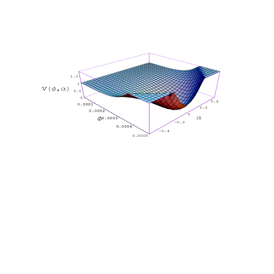
Figure 1: (a) The inflationary potential (in units of $V_{0}\equiv\Delta^{4}$) Eq.(6), is shown as a function of the magnitud of $\phi$, denoted again by $\phi$, and its phase $\alpha$ for the case $(p,q)=(4,2)$, $\mu=0.024$ and ${\kappa}=1$. We notice that $\alpha=0$ is a stable direction of the potential. The height of the potential corresponds to a scale of $4.6{\times}10^{11}$ GeV.
(b) Notice that $<\phi_{0}>\sim 10^{-4}\ll 1$, thus Eq.(9) remains a good approximation for the whole potential.

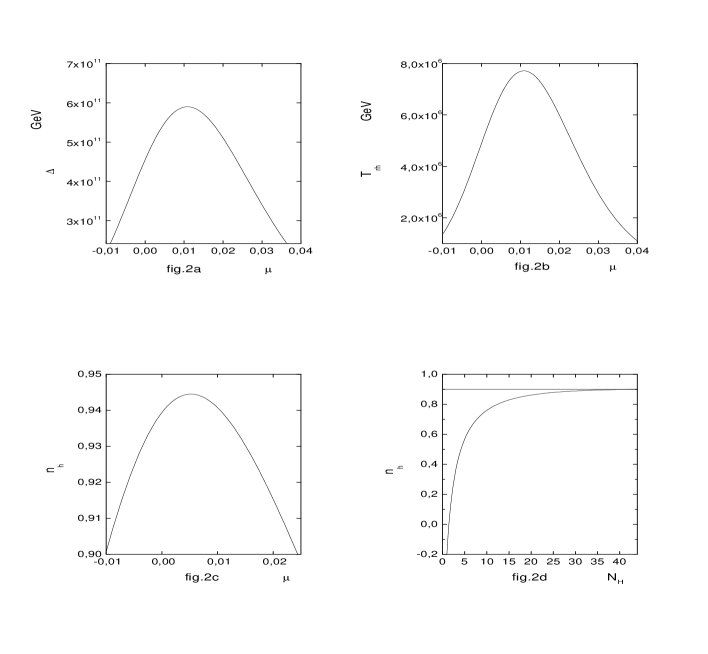
Figure 2: The scale of inflation $\Delta$ given by Eq.(19) is shown in Fig. 2a as a function of $\mu$ for the case $(p,q)=(4,2)$, $N_{{\rm H}}=48$ and $\kappa=1$. Similar behaviour occurs for the other $(p,q)$ cases although with different maximum values. Fig. 2b: The reheat temperature $T_{rh}$ given by Eq.(25) is shown as a function of $\mu$ for the case $(p,q)=(4,2)$, $N_{{\rm H}}=48$ and $\kappa=1$. Fig. 2c: The spectral index Eq.(20) is shown as a function of $\mu$ for the case $(p,q)=(4,2)$, $N_{{\rm H}}=48$ and $\kappa=1$. Note that there is a maximum value which $n_{{\rm H}}$ can have. The same behaviour occurs for the other $(p,q)$ cases although with different maximum values. Fig. 2d: The spectral index Eq.(20) is shown as a function of the number $N_{{\rm H}}$ of e-folds of inflation from the end of inflation as the origin, where it takes a value $-1$. This figure corresponds to the case $(p,q)=(4,2)$, $\mu=0.024$ and $\kappa=1$.The horizontal line correspond to $n_{{\rm H}}=0.9$. Similar shapes are found in the other $(p,q)$ cases.

We now plot in $Fig.1$ the inflaton potential $V(\phi,\alpha)$ as a function of $\phi$ and the phase $\alpha$. In $Figs.2a,2b$, and $2c$ we plot the scale of inflation $\Delta$, the reheating temperature $T_{rh}$, and the spectral index $n_{{\rm H}}$ as functions of the parameter $\mu$, respectively. Finally $Fig.2d$ shows the behaviour of the spectral index as a function of the number $N_{{\rm H}}$ of e-folds of inflation from the end of inflation. All of these figures are for the case $(p,q)=(4,2)$. Similar behaviour is found in the other $(p,q)$ cases.

5 Comparison with related work

In the models studied in [1] and further elaborated in [5] quadratic inflation is implemented through a hybrid mechanism with the participation of two fields. A linear term in a field $Y$ follows if $Y$ carries non-zero $R$-symmetry charge under an unbroken $R$-symmetry. The inflaton $\phi$ is a singlet under the $R$-symmetry but carries a charge under a discrete $Z_{p}$ symmetry. Then the superpotential has the form

$$W=\left(\Delta^{2}-\frac{\phi^{p}}{M^{\prime p-2}}-\frac{\phi^{2p}}{M^{\prime 2p-2}}-\dots\right)Y.$$ (28)

This gives rise to the potential

$$V=\left(\Delta^{2}-\frac{\phi^{p}}{M^{\prime p-2}}-\frac{\phi^{2p}}{M^{\prime 2p-2}}-\dots\right)^{2},$$ (29)

displaying the possibilities of ending inflation. There are also terms involving $Y$ which are dropped as they do not contribute to the vacuum energy since $Y$ does not acquire a vacuum expectation value. The scale $M^{\prime}$ denotes new physics below the Planck scale and we can write $M^{\prime p-2}=\Delta^{q}M^{p-q-2}$ to take into account the possibility that the scale associated with the higher dimension operators may be below the Planck scale.

In the present model there is only a single scalar field with a superpotential determined by the $R$-symmetry as shown in Section 2. As a consequence of this symmetry some $(p,q)$ models which occur in [1], [5] (for example $(p,q)=(4,3)$) are not allowed here. It is therefore interesting that most of the results and conclusions of [1] are still maintained.

Other studies of quadratic inflation have concentrated on the case where radiative corrections make the potential develop a maximum near the origin, from which the inflaton rolls either away from the origin or towards it [13], and inflation ends through a hybrid mechanism.

There is also related work [4] with a superpotential (in our notation)

$$W(\phi)=\Delta^{2}\phi-\frac{\kappa}{n}\phi^{n},$$ (30)

and the Kähler potential

$$K(\phi,\phi^{*})=\phi\phi^{*}+\frac{\mu}{4}(\phi\phi^{*})^{2}+...,$$ (31)

where $\phi$ and $\Delta$ have R-charges as in Eq.(3). However the fact that the factor $\Delta^{-q}$ appearing in our Eq.(1) is not present in Eq.(30) above eliminates the possibility of having low scales for inflation (in [4] the lowest scale allowed is ${\cal O}(10^{12}GeV)).$

6 Conclusions

We have studied a model of inflation where low inflationary scales are allowed without having to introduce unnatural values for the parameters involved. The model is defined in terms of a single scalar field, the inflaton, and the term driving (new) inflation is quadratic in $\phi$. The end of inflation due to higher order non-renormalisable terms. Radiative corrections to the inflaton mass reduce $m_{\phi}^{2}$ from its natural value at the Planck scale. For a light inflaton thermal initial conditions can naturally place the inflaton at the origin, initiating a (last) stage of new inflation. A quadratic parameterisation of the inflationary potential allows low values for the inflationary scale $\Delta$. One can have $\Delta\sim 10^{10}~{}{\rm GeV}$, the supersymmetry breaking scale in the hidden sector or the electroweak scale $\Delta\sim 10^{3}~{}{\rm GeV}$ which could be relevant in the context of theories with submillimeter dimensions. The well justified assumption that the inflaton mass parameter $m_{\phi}^{2}\sim\mu\Delta^{4}$ remains practically constant during inflation allows analytical closed form expressions for all the relevant quantities.

7 Acknowledgements

G.G. would like to thank G.G. Ross and S. Sarkar for useful discussions. This work was supported by the projects PAPIIT IN110200, and Conacyt 32415-E.

References

- [1] G. Germán, G.G. Ross and S. Sarkar, Phys. Lett. 469B (1999) 46.
- [2] A.D. Linde, Phys. Lett. 108B (1982) 389; A. Albrecht and P.J. Steinhardt, Phys. Rev. Lett. 48 (1982) 1220.
- [3] N. Arkani-Hamed, S. Dimopoulos, G. Dvali, Phys. Lett. 429B (1998) 263; I. Antoniadis, N. Arkani-Hamed, S. Dimopoulos, G. Dvali, Phys. Lett. 436B (1998) 257; N. Arkani-Hamed, S. Dimopoulos, J. March-Russell, hep-th/9809124.
- [4] K.I. Izawa, and T. Yanagida, Phys. Lett. B393 (1997) 331.
- [5] G. Germán, G.G. Ross and S. Sarkar, in preparation.
- [6] K. Kumekawa, T. Moroi, and T. Yanagida, Prog. Theor. Phys. 92 (1994) 437.
- [7] D. Bailin and A. Love, Supersymmetric Gauge Field Theory and String Theory (Adam Hilger, 1994).
- [8] For a review and extensive references, see, D.H. Lyth and A. Riotto, Phys. Rep. 314 (1999) 1.
- [9] C.L. Bennett et al (COBE collab.), Astrophys. J. 464 (1996) L1.
- [10] A.D. Linde, Particle Physics and Inflationary Cosmology (Harwood Academic Press, 1990).
- [11] P.J. Steinhardt, M.S. Turner, Phys. Rev. D29 (1984) 2162.
- [12] For a review, see, A.R. Liddle and D.H. Lyth, Phys. Rep. 231 (1993) 1.
- [13] E.D. Stewart, Phys. Lett. B391 (1997) 34, Phys. Rev. D56 (1997) 2019; L. Covi, D.H. Lyth and L. Roszkowski, Phys. Rev. D60 (1999) 023509; L. Covi and D.H. Lyth, Phys. Rev. D60 (1999) 063515; L. Covi, Phys. Rev. D60 (1999) 023513.