PUPT-1936

hep-th/0006119

Phase structure of non-commutative
scalar field theories

S. S. Gubser and S. L. Sondhi

Joseph Henry Laboratories, Princeton University, Princeton, NJ 08544

Abstract

We investigate the phase structure of non-commutative scalar field theories and find evidence for ordered phases which break translation invariance. A self-consistent one-loop analysis indicates that the transition into these ordered phases is first order. The phase structure and the existence of scaling limits provides an alternative to the structure of counter-terms in determining the renormalizability of non-commutative field theories. On the basis of the existence of a critical point in the closely related planar theory, we argue that there are renormalizable interacting non-commutative scalar field theories in dimensions two and above. We exhibit this renormalization explicitly in the large $N$ limit of a non-commutative $O(N)$ vector model.

June 2000

1 Introduction

Non-commutative field theories have recently received a great deal of attention [1, 2, 3, 4, 5, 6, 7, 8], stemming in part from the fact that they arise as low-energy descriptions of string backgrounds with anti-symmetric tensor fields [4]. Renormalizability of non-commutative theories remains an open question. Standard approaches to demonstrating perturbative renormalizability (see for instance [5]) encounter difficulties because of infrared singularities. These singularities are not associated with any massless propagating fields in the theory, but instead arise through loop effects. They can have dramatic physical consequences: for instance, in a theory whose classical action is that of a massive scalar with cubic interactions, the $\phi=0$ vacuum becomes not just globally unstable (on account of an effective potential which is unbounded below), but locally unstable, as if the scalar had become tachyonic [6].

The main interest in this paper will be in scalar theories with $\phi^{4}$ interactions. For the most part we will restrict attention to Euclidean signature and to even dimensions. Following [6], we will briefly review in Section 3.2 how non-planar one-loop graphs lead to a singularity in the one particle irreducible (1PI) two-point function: $\Gamma^{(2)}(p)\to\infty$ as $p\to 0$. What this amounts to physically is long-range frustration: $\langle\phi(x)\phi(0)\rangle$ oscillates in sign for large $x$. A natural expectation, given such a correlator, is that the usual Ising-type phase transition, to an ordered phase with $\langle\phi\rangle\neq 0$, will be modified to a transition to a phase where $\langle\phi\rangle$ varies spatially. This is indeed what we will find in Section 4: more particularly, we will find a fluctuation-driven first order transition to a stripe phase, where only one momentum mode of the scalar field condenses. In Section 4.6 we will consider more complicated ordered phases, where more than one momentum mode condenses. In the perturbative regime of Section 4, it turns out that stripe phases are favored; however, it appears that as couplings are increased, the system alternates between preferring the condensation of one or several momentum modes.

The overall picture we will find for the phase diagram is a first order line terminating on one end at a Lifshitz point, where first order behavior merges back into the second order transition of the Ising model; and terminating on the other end at a critical point which arises in a planar version of the commutative theory. We review in Section 2 the relationship between phase structure and renormalizability, and argue via scaling that the existence of the critical point in the planar theory should imply the renormalizability of the non-commutative theory.

The main method we use to establish the existence of phase transitions is a self-consistent Hartree treatment of one-loop graphs. This same method is our primary tool in demonstrating the validity of the scaling arguments that guarantee renormalizability. Thus, these arguments are airtight only for the large $N$ limit of a non-commutative $O(N)$ vector model, where the self-consistent one-loop Hartree treatment becomes exact. More sophisticated methods are called for to decide the validity of scaling relations in more general non-commutative field theories. As explained in Section 5, it is possible to arrange the quartic couplings in the $O(N)$ theory so that there are no divergences at all at leading order in $N$, independent of the dimension. Our renormalizability arguments apply, however, for arbitrary quartic couplings in the $O(N)$ theory.

Other authors [13, 14, 15] have discussed finite temperature effects in non-commutative field theories, using the Matsubara formalism with periodic Euclidean time. The aim of this paper is rather different: we work with non-commutative field theories on uncompactified flat space, and varying “temperature” is regarded as equivalent to changing the bare mass.

We conclude in Section 7 with a discussion of the relevance of our results to string theory and to quantum hall systems.

2 Phase Structure and Renormalizability

We begin with an extremely brief recapitulation of the Wilsonian connection between the phase structure of a (cutoff) field theory and that of taking its continuum limit—which is the problem of renormalizability. As we are interested in this paper in the renormalization of scalar fields, we will recall the lore on commuting scalar fields.

Figure 1: The phase diagram for the Ising scalar field theory, (1), in $d>1$.

In the Wilsonian approach, we study the Euclidean field theory governed by the action

$$S=\int d^{d}x\left[{1\over 2}(\partial\phi)^{2}+{1\over 2}m^{2}\phi^{2}+{g^{2}\over 4}\phi^{4}\right]$$ (1)

as a statistical mechanics problem—i.e. we introduce a momentum cutoff $\Lambda$ and measure all dimensionful quantities in its units. This leaves us with a problem with one degree of freedom per dimensionless volume ($\Lambda^{-d}$ in physical units) and dimensionless couplings $m^{2}/\Lambda^{2}$ and $g^{2}/\Lambda^{4-d}$, commonly labelled $r$ and $u$ in the statistical mechanics/condensed matter literature (see for instance [16]). We next search for lines of continuous phase transitions, or critical surfaces, in the $r,u$ plane; the critical surface in this problem (which is in the universality class of the Ising model) is sketched in Figure 1. On this surface, the correlation length, in dimensionless units, $\xi$ (the “lattice” correlation length, literally so if the cutoff is implemented via discretization) diverges which is the sine qua non of taking a continuum limit. Having located a critical surface, three continuum limits are possible at each point on it—a massless limit obtained by sitting exactly on the critical surface, and two massive limits in which $r(\Lambda)$ and $u(\Lambda)$ are chosen to approach the critical surface from either phase as the cutoff is taken to infinity while keeping $\Lambda/\xi(r,u)=M_{R}$ fixed and equal to a renormalized mass. That such limits can be taken, requires scaling in the statistical mechanics. Also, the phenomenon of universality will imply that some domain of a critical surface will exhibit the same long distance correlations and hence give rise to the same continuum limit.

Figure 2: Renormalization group flows for the Ising scalar field theory in (a) $d=4$ and (b) $d<4$.

In the above description we have used the language of phase structure. A more powerful account is that of renormalization group (RG) flows which we have sketched in $d=4$ (Figure 2a) and $d<4$ (Figure 2b). In the RG description we are interested in fixed points of infinite correlation length. In $d=4$ we see that all critical theories flow into the gaussian fixed point $(r,u)=(0,0)$ whence the (strict) continuum limit is trivial, while in $d<4$ the non-trivial Wilson-Fisher fixed point leads to an interacting continuum limit. This information is not available from a phase diagram alone. The fixed point analysis also implies scaling and hence guarantees a continuum limit.

We belabor this point because in the balance of the paper, we will deal in phase diagrams and not RG flows. We will find critical points and will argue that these guarantee the existence of continuum limits (renormalizability) of non-commuting scalar theories. In a specific large $N$ theory, we will be able to show this explicitly, and we do not doubt that the claim is correct. Nevertheless, it does not have the full generality of an RG analysis and it would be nice to carry out such an analysis, even perturbatively as done for the commutative $\phi^{4}$ theory in $d=4$ by Polchinski [17].

3 One Loop Action for Non-Commutative Scalars

3.1 Generalities

Our starting point is the non-commutative scalar field theory specified by the action

$$S=\int d^{d}x\left[{1\over 2}(\partial\phi)^{2}+{1\over 2}m^{2}\phi^{2}+{g^{2}\over 4}\phi^{\star 4}\right]$$ (2)

where $\phi^{\star 4}=\phi\star\phi\star\phi\star\phi$ and the star product is defined as usual by

$$(f\star g)(x)=\left.e^{{i\over 2}\Theta^{\mu\nu}\partial_{x^{\mu}}\partial_{y^{\nu}}}f(x)g(y)\right|_{y=x}\,.$$ (3)

The anti-symmetric matrix $\Theta^{\mu\nu}$, whose relation to the star product can be most simply expressed through

$$[x^{\mu},x^{\nu}]_{\star}\equiv x^{\mu}\star x^{\nu}-x^{\nu}\star x^{\mu}=i\Theta^{\mu\nu}\,,$$ (4)

will for most of this paper be assumed to be of the form

$$\Theta^{\mu\nu}=\theta\pmatrix{0&1\cr-1&0}\otimes{\bf 1}_{d/2}$$ (5)

for even dimensions $d$. We will comment in Section 4.5 on the more complicated cases where $\Theta^{\mu\nu}$ has unequal eigenvalues or $d$ is odd.

A useful extension of (3) is

$$(f_{1}\star f_{2}\star\ldots\star f_{\ell})(x)=\left.e^{{i\over 2}\sum_{i<j}\Theta^{\mu\nu}\partial_{x_{i}^{\mu}}\partial_{x_{j}^{\nu}}}f_{1}(x_{1})f_{2}(x_{2})\cdots f_{\ell}(x_{\ell})\right|_{x_{i}=x}\,.$$ (6)

The result (6) is easiest to obtain via Fourier analysis, using the basic result

$$e^{ip_{1}\cdot x}\star e^{ip_{2}\cdot x}=e^{-{i\over 2}p_{1}\wedge p_{2}}e^{i(p_{1}+p_{2})\cdot x}\,,$$ (7)

where by definition $p\wedge q=\Theta^{\mu\nu}p_{\mu}p_{\nu}$. (Condensed matter readers should note that this is the lowest Landau level algebra of density operators [18]).

Like matrix multiplication, the star product is non-commutative. However, a product of exponentials $e^{ip_{k}\cdot x}$, can be reordered cyclically if the $p_{k}$ sum to zero. As a result it is necessary to specify the cyclic order of vertices in writing down Feynman rules, just as in large $N$ theories. It is well known [1] that planar amplitudes of the field theory (2) are independent of $\Theta^{\mu\nu}$ (and hence are the same as in the commutative theory where $\Theta^{\mu\nu}=0$), up to an overall phase. The effects of non-planar diagrams were first studied systematically in [6].

We will also consider two variants of (2), namely complex scalars, where

$$S=\int d^{d}x\,\left[\partial\phi\partial\phi^{*}+m^{2}\phi\phi^{*}+g^{2}\phi\star\phi^{*}\star\phi\star\phi^{*}+g^{\prime 2}\phi\star\phi\star\phi^{*}\star\phi^{*}\right]\,,$$ (8)

and the non-commutative $O(N)$ vector model,

$$S=\int d^{d}x\,\left[{1\over 2}(\partial\phi_{i})^{2}+{1\over 2}m^{2}\phi_{i}^{2}+{g^{2}\over 4}\phi_{i}\star\phi_{i}\star\phi_{j}\star\phi_{j}+{g^{\prime 2}\over 4}\delta^{ik}\delta^{jl}\phi_{i}\star\phi_{j}\star\phi_{k}\star\phi_{l}\right]$$ (9)

The field theory (8) has been studied previously [19].

3.2 One loop diagrams

In this section we review the results of [6] which will be relevant for our calculations. The one loop corrections to the propagator of the scalar field $\phi$ split into planar and non-planar parts:

$${\Sigma_{\rm planar}(p)}$$

(10)

Using the Schwinger parametrization

$${1\over k^{2}+m^{2}}=\int_{0}^{\infty}d\alpha\,e^{-\alpha(k^{2}+m^{2})}\,,$$ (11)

one easily extracts

$${I_{2}(p)}$$

(12)

where, following [6], we have introduced an ultraviolet regulator $\Lambda$ and defined a symmetric product

$$p\circ q=-p_{\mu}\Theta^{\mu\nu}\Theta_{\nu}{}^{\lambda}q_{\lambda}\,.$$ (13)

$K_{\nu}(x)$ denotes a modified Bessel function.

The end result is a corrected propagator of the following form:

$$\Gamma^{(2)}(p)=p^{2}+m^{2}+2g^{2}I_{2}(0)+g^{2}I_{2}(p)\,.$$ (14)

The parallel results for the complex scalar and the $O(N)$ vector model are

complex scalar: $${{}\Gamma^{(2)}(p)=p^{2}+m^{2}+(2g^{2}+g^{\prime 2})I_{2}(0)+g^{\prime 2}I_{2}(p)}$$

model:

(15)

where for the $O(N)$ model we have only evaluated the graphs which contribute at leading order in large $N$. The salient property of $\Gamma^{(2)}(p)$ for our subsequent discussion is that it grows for small $p$. If we think of absorbing the planar one-loop contribution to $\Gamma^{(2)}(p)$ into the definition of mass (for instance, define a renormalized mass through $M^{2}=m^{2}+2g^{2}I_{2}(p^{2})$ for the real scalar theory), and then removing the cutoff while holding $M^{2}$ fixed, then $\Gamma^{(2)}(p)$ is finite for finite $p$ but goes to $+\infty$ as $p\to 0$. This means that the low-momentum modes are extremely stiff; thus they seem likely never to participate in a phase transition. If there is a phase transition, it should involve the momentum modes where $\Gamma^{(2)}(p)$ is smallest, since these are the ones most likely to be destabilized as $M^{2}$ becomes negative. The details of how this happens turn out to be somewhat intricate, and the next section is devoted to sorting them out.

4 Phase Structure for Non-commutative scalars

4.1 Generalities

The non-commutative action (2) is characterized by three dimensionless parameters: $m^{2}/\Lambda^{2}$, $g^{2}/\Lambda^{4-d}$ and $\theta\Lambda^{2}$. Accordingly we need to establish a phase diagram in a three dimensional space. In what follows we will typically work at a fixed dimensionless coupling and take two dimensional cuts through parameter space instead. The resulting phase diagram is sketched in Figure 3, and the rest of this section is devoted to the arguments that give rise to it.

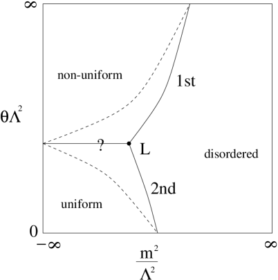
Figure 3: The phase diagram for the non-commutative $\phi^{4}$ theory at fixed $g^{2}$, in $d=4$. The solid lines show transitions for the case of a single real scalar. The point marked L is a Lifshitz point. The transition between uniform and non-uniform ordered phases is not accessible, in $d=4$, via the techniques used in this paper. Instead, the dashed lines represent the transitions that arise in a self-consistent one-loop analysis.

4.2 The Planar Limit: $\theta\Lambda^{2}=\infty$

It has been noted previously that the large $\theta$ limit picks out planar diagrams [1]. In the context of a cutoff field theory, this statement can be made precise.

Consider the theory at $m^{2}/\Lambda^{2}>0$ so that all diagrams are infrared finite in addition to being ultraviolet finite on account of the cutoff. The perturbative expansion for the free energy $F=-\log Z$ is the sum of all connected vacuum diagrams (no external legs). Of these, the planar graphs involve no phase factors stemming from the non-commutativity while the non-planar graphs involve at least one. In the limit $\theta\Lambda^{2}\rightarrow\infty$ the latter vanish on account of the infinitely rapid oscillations of the integrand. Consequently, the high temperature expansion of $F$ in the maximally non-commuting scalar theory is identical to that of the planar theory, defined as the sum over planar diagrams alone.

This statement can be extended to selected classes of fields. The perturbative expansion for the free energy in a field is,

$${-F[J]}$$

(16)

where $G_{c}(p_{1},....,p_{n})$, inclusive of the momentum conserving delta function, is the connected $n$-point Green function in momentum space. On account of the vanishing of the non-planar graphs alluded to earlier,

$$\lim_{\theta\Lambda^{2}\rightarrow\infty}e^{{i\over 2}\sum_{i<j}p_{i}\wedge p_{j}}G_{c}(p_{1},....,p_{n};\theta\Lambda^{2})=G_{c}^{\rm planar}(p_{1},....,p_{n})$$ (17)

for each $n$. For fields that are modulated only in one direction, the momenta $p_{1}$ through $p_{n}$ are parallel whence the explicit phase factor for planar diagrams vanishes. Hence in the limit $\theta\Lambda^{2}\rightarrow\infty$, $F[J]$ is still given as a sum of planar diagrams alone. Note that for more complicated field configurations, the equivalence is no longer true.

Thus far we have made statements in the high temperature phase. The planar theory, inheriting the Ising symmetry ($\phi\to-\phi$) of the full theory, will exhibit a twofold degenerate broken symmetry phase. This will be reached on traversing a continuous phase transition at a critical $m_{c}^{2}/\Lambda^{2}<0$ which will be mean field in $d>4$, mean field corrected by logarithms in $d=4$, but likely in a different universality class from the standard Ising transition in $d<4$ (see below). An immediate deduction from the equivalence of the infinite $\theta\Lambda^{2}$ and planar theories in a field is that we may analytically continue their common free energy into the low temperature phase (bypassing the critical point), thereby establishing the equivalence of their low temperature thermodynamics as well. Altogether, we may conclude that the infinite $\theta\Lambda^{2}$ theory has a critical point at the same $m_{c}^{2}/\Lambda^{2}$ as the planar theory, which is exactly the same transition. This critical point will play a central role in achieving a continuum limit for the noncommutative theory.

Finally we should note the well known result that the planar theory is also the $N\rightarrow\infty$ limit of a hermitian matrix model with an appropriately generalized version of (1) as its action. Via this route, there are exact results on the phase transition in $d=1$ [20] that show that the transition is different from that of the Ising model, and an approximate RG treatment that has yielded exponents in $2<d<4$ as well [21, 22]. There does not appear to be a treatment of the broken symmetry phase in this formulation of the problem—at issue is how the Ising symmetry of the planar theory is embedded in what appears prima facie to be a much larger symmetry group in the matrix model.

4.3 First Order Transition at Large $\theta\Lambda^{2}$

Having established that there is a critical point at $\theta\Lambda^{2}=\infty$, we will now show that this terminates a line of fluctuation driven first order transitions at large $\theta\Lambda^{2}$. That this should happen, is a fairly general expectation from the work of Brazovskii [23] when combined with the observation [6] that the one loop $\Gamma^{(2)}(p)$ has a minimum at non-zero $p$ at large $\theta\Lambda^{2}$ (the latter condition is implicit in their analysis), and we will review this physics below. Following Brazovskii, we will employ the self-consistent Hartree approximation. This approximation is sensible in $d\geq 4$, but does not capture the planar theory transition in $d=2$. Consequently, we will not treat that case in detail, although our later arguments on renormalizability will apply there as well.

We will present two separate arguments for the first order transition. The first will involve an asymptotic construction of the solution to the self-consistent problem—this will follow the original analysis as closely as possible but with complications that we detail below. This will also require that we take a double limit in which $\theta\Lambda^{2}$ is taken large but $g^{2}$ is taken to zero—i.e. we will be working in the vicinity of the massless Gaussian theory. The second will be a more indirect argument which will be carried out at fixed $g^{2}$ and will consist of showing that the free energy of two solutions must cross in a certain region of parameter space.

4.3.1 Take I

We turn to the direct construction. To keep the discussion simple, we will continue to assume even Euclidean dimension $d$, and $\Theta^{\mu\nu}$ with maximal rank and eigenvalues $\pm\theta$. We will also omit inessential factors of order unity.

A self-consistent treatment of the one-loop correction to the propagator leads to

$$\Gamma^{(2)}(p)=p^{2}+m^{2}+2g^{2}\int{d^{d}k\over(2\pi)^{d}}{1+{1\over 2}e^{ik\wedge p}\over\Gamma^{(2)}(k)}$$ (18)

Having $\Theta^{\mu\nu}$ of maximal rank, with eigenvalues $\pm\theta$, leads to a considerable simplification: $\Gamma^{(2)}(p)$ is a function only of $p^{2}$. This can be shown inductively, order by order in $g^{2}$. Suppose that $\Gamma^{(2)}(p)$ is $SO(d-1)$ to $\ell$-th order in $g^{2}$. The $(\ell+1)$-st order expression for $\Gamma^{(2)}(p)$ is then invariant on $SO(d-1)$ transformations of $p_{\mu}\Theta^{\mu\nu}$, and so can only be a function of $p\circ p=\theta^{2}p^{2}$. Equation (18) can thus be re-expressed as

$$\Gamma^{(2)}(p)=p^{2}+M^{2}+g^{2}\int_{0}^{\infty}k^{d-1}dk{J_{(d-2)/2}(\theta kp)\over(\theta kp)^{(d-2)/2}}{1\over\Gamma^{(2)}(k)}\,.$$ (19)

Here $m^{2}$ is the bare mass, and

$$M^{2}=m^{2}+2g^{2}\int{d^{d}k\over(2\pi)^{d}}{1\over\Gamma^{(2)}(k)}$$ (20)

is the mass corrected by the planar graph, Figure 4a. The non-commutativity does not affect the large $p$ behavior, $\Gamma^{(2)}(p)\sim p^{2}$. Thus the integral in (20) must be regulated, for instance with an explicit cutoff as in Section 3.2. No other ultraviolet divergences will arise in the following computations, so we may in effect take the cutoff to infinity and treat $M^{2}$ as the finite quantity which we dial to produce a transition. This leads to an argument for renormalizability, as we shall explain in Section 6.

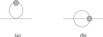
Figure 4: 1PI graphs with dressed propagators.

The last term in (18) has a contribution from large momenta $k$ which goes as $1/p^{d-2}$ as $p\to 0$. This prevents condensation of very low-momentum modes of $\phi$. Thus, if there is a phase transition at all, the ordered state must break translation invariance.

From now on, let us restrict attention to $d=4$. At the end of this section we will remark on the extension to other dimensions. Proceeding naively, we could solve (19) to the first non-trivial order in $g$ by replacing $\Gamma^{(2)}(k)$ on the right hand side by $k^{2}+M^{2}$. Then as $M^{2}$ is decreased below $-c_{1}{g\over\theta}$, for some (easily computable) constant $c_{1}$ of order unity, $\Gamma^{(2)}(p)$ becomes negative near $p=p_{c}\sim\sqrt{g/\theta}$, signalling a second order phase transition to an ordered state where some momentum modes of $\phi$ condense. Our aim in the rest of this subsection is to show that this naive result is altered in a self-consistent analysis to a rather more interesting conclusion: there is a first order transition to a stripe pattern at $M^{2}=-c_{1}{g\over\theta}-c_{2}{g^{7/3}\over\theta}$, where $c_{2}$ is another constant of order unity.

First observe that (19) makes the second order transition impossible. If we were to suppose that $\Gamma^{(2)}(p_{c})=0$ for some $M^{2}$ and some $p_{c}$, then the integral in (19) diverges. The possibility of a first order transition was first realized by Brazovskii [23], given a suitable effective Lagrangian, with a minimum in the inverse propagator at non-zero $p_{c}$. In [23], such an effective Lagrangian was simply assumed, and a one-loop fluctuation analysis with this starting point was shown to lead to a first order transition. This same method was further developed in [24]. In our case, the basic Lagrangian does not have an appropriate inverse propagator with a minimum at nonzero $p_{c}$—as we have seen, this only arises in the 1PI effective action after a one-loop analysis. One cannot feed $\Gamma^{(2)}(p)$ directly into a Brazovskiian analysis: all fluctuations are supposed to be incorporated into $\Gamma^{(2)}(p)$ already. However, we shall see that a self-consistent treatment based on (19) reproduces the essential features of [23], and does support the conclusion that a first order transition takes place.

Although $\Gamma^{(2)}(p)$ can never vanish, it should be possible to make its minimum as small as we please by decreasing $M^{2}$ sufficiently. We then have the approximate forms

$${\Gamma^{(2)}(p)} {{}\approx p^{2}} p {\Gamma^{(2)}(p)} {{}\approx\xi_{0}^{2}(p^{2}-p_{c}^{2})^{2}+r} p\approx p_{c} {\Gamma^{(2)}(p)} {{}\approx{g^{2}\over(\theta p)^{2}}} p$$ for large for for small . (21)

Two regions of the integral in (19) will then make significant contributions: the large $p$ region and the $p\approx p_{c}$ region. The full integral can be approximated as a sum of the contributions from these regions. The parameters $p_{c}$ and $\xi_{0}$ can then be determined self-consistently: for $p\approx p_{c}$,

$${\Gamma^{(2)}(p)}$$

(22)

The last line of (22) follows from matching the previous line to the approximate form $\Gamma^{(2)}(p)\approx\xi_{0}^{2}(p^{2}-p_{c}^{2})^{2}$. We have again suppressed inessential factors of order unity in (22), and we have assumed $g\ll 1$, so that $\theta p_{c}^{2}\ll 1$. This latter inequality will be essential to our further analysis. It turns out to be difficult to get the factors of order unity right, because $\xi_{0}$ is only on the order of $1/p_{c}$: the breadth of the minimum of $\Gamma^{(2)}(p)$, in the approximation scheme we have used, is comparable to its distance from the origin.

So far we have done all calculations as expansions around the disordered phase, where $\langle\phi\rangle=0$. The putative ordered phase is a stripe pattern: $\langle\phi\rangle=\phi_{0}=A\cos p_{c}x$. (Strictly speaking, we do not expect an exact $\cos p_{c}x$ dependence, only a function of $x$ with period $2\pi/p_{c}$. But because the momentum modes near $p_{c}$ make the dominant contribution, neglecting higher harmonics should not change the qualitative picture. One should in principle consider sums of the form $\cos p_{c}x+\cos p_{c}y$, as well as more complicated superpositions; however, as we shall see in Section 4.6, the simple stripe solution is favored at small coupling). Writing $\phi=\phi_{0}+\eta$ and expanding in fluctuations of $\eta$, one obtains

$${{\cal L}}$$

(23)

We will treat perturbatively all terms with factors of both $\eta$ and $\phi_{0}$. This is justified if $A$ is small, which is not completely obvious given that the transition is first order. But for small $g$, $A$ is small very close to the phase transition—at least, this is an assumption which can easily be verified at the end of the computation.

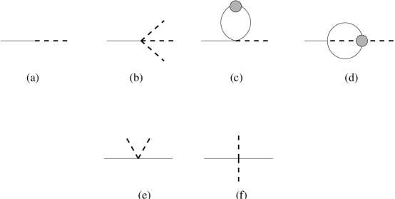
Figure 5: Additional 1PI graphs for the ordered phase. Dashed external lines indicate insertions of the background field $\phi_{0}$.

Classically, one would demand that the terms in (23) linear in $\eta$ should vanish: this corresponds to summing the graphs in Figure 5a and 5b. At the one-loop level, the graphs in Figure 5c and 5d also contribute, and the end result is

$$h\equiv{1\over 2}{d\Phi\over dA}=\Gamma^{(2)}(p_{c})A-{g^{2}\over 2}A^{3}\,,$$ (24)

where $\Phi$ is the free energy per unit volume. Adding the graphs in Figures 5e and 5f to the self-consistent one-loop graphs that contributed to (18), one finds only a slight modification of the propagator in the disordered phase: To (18) one must simply add the terms $g^{2}A^{2}(1+{1\over 2}\cos p\wedge p_{c})$. The first of these terms comes from the graph in Figure 5e, while the second is from the graph in Figure 5f. For momenta $p$ on the order of $p_{c}$, the argument of the cosine is small (again assuming $\theta p_{c}^{2}$ is small), so for such momenta we may alter (22) to

$${\Gamma^{(2)}(p)}$$

(25)

To summarize the situation so far: a self-consistent analysis of the graphs in Figures 4 and 5 led to an expression for the minimum, $r=\Gamma^{(2)}(p_{c})$, of the 1PI propagator $\Gamma^{(2)}(p)$; and an expression for the tadpole for the magnitude $A$ of the condensate. These expressions are

$$r=\tau+g^{2}A^{2}+{\alpha\over\sqrt{r}}\qquad{1\over 2}{\partial\Phi\over\partial A}=A\left(r-{g^{2}\over 2}A^{2}\right)\,,$$ (26)

where we have defined

$$\tau=2p_{c}^{2}+M^{2}\qquad\alpha={g^{7/2}\over\theta^{3/2}}\qquad p_{c}=\sqrt{g\over\theta}\,.$$ (27)

The various factors of order unity which we have neglected can be absorbed by rescaling $g$, $p_{c}$, and $\alpha$. None of these rescalings affects the conclusion that there is a first order transition. However, the rest of the analysis is somewhat delicate, and we must from now on be meticulous about factors. The calculation we are about to sketch appeared in [23] with some slight errors, which were corrected in [25], modulo a typo in the sign of the last term in their (2.13).

A stable phase must have a vanishing tadpole. This happens either when $A=0$ (the disordered phase) or when $r-{g^{2}\over 2}A^{2}=0$ (the ordered phase). The respective values of $r$, as well as the value of $A$ in the ordered phase, can be determined from

$${r_{o}+{\alpha\over\sqrt{r_{o}}}+\tau=0\qquad r_{d}-{\alpha\over\sqrt{r_{d}}}-\tau=0} {A_{o}={1\over g}\sqrt{r_{o}-{\alpha\over\sqrt{r_{o}}}-\tau}\,.}$$ (28)

Note that the ordered phase only exists for $\tau<-3(\alpha/2)^{2/3}\approx-1.89\alpha^{2/3}$. In this range, there are two solutions for $r_{o}$ (both positive): let us call these $r_{o1}$ and $r_{o2}$. The free energy difference is conveniently calculated as

$${\Delta\Phi}$$

(29)

This equation applies equally to the two solutions for $r_{o}$. By subtracting (29) with $r_{o}=r_{o1}$ from the same equation with $r_{o}=r_{o2}$, one can verify that the larger solution for $r_{o}$ leads to the lower free energy. One can also show, directly from (29), that the disordered phase is favored for $-2.03\alpha^{2/3}<\tau<-1.89\alpha^{2/3}$, and the ordered phase is favored for $\tau<-2.03\alpha^{2/3}$.

In terms of the original variables, and again in $d=4$, the phase transition to an ordered phase occurs when $M^{2}=-c_{1}{g\over\theta}-c_{2}{g^{7/3}\over\theta}$, for some constants $c_{1}$ and $c_{2}$ of order unity. It is straightforward to show that $c_{1}=1/\pi$ and $\theta p_{c}^{2}=g/2\pi$. But to obtain an accurate value for $c_{2}$ requires numerics. The $g^{7/3}$ correction is a measure of the extent to which the system avoids the second order behavior expected from a naive one-loop analysis. Higher loop corrections are expected to shift the critical value of $M^{2}\theta$ by $O(g^{3})$.

4.3.2 Take II

We now consider a second route to establishing a first order transition at large $\theta\Lambda^{2}$ which exploits the intimate connection between the phases of the noncommutative theory and their limits in the planar theory. The basic idea is this: As shown earlier, one cannot have a continuous transition once the disordered phase propagator has a minimum away from zero which is the case once $\theta\Lambda^{2}$ is reduced from infinity. While this allows the high temperature solution to exist below the critical temperature of the planar theory, there must be a second solution that grows out of the ordered solution of the planar theory but is now modulated at a very long wavelength. If we take $\theta\Lambda^{2}$ sufficiently large at fixed $m^{2}<m_{c}^{2}$, the ordered solution will win for it is the correct solution at $\theta\Lambda^{2}=\infty$. Hence there must be a first order line emanating from the planar theory critical point.

To construct a proof on these lines it would appear that we could get away by comparing free energies exactly at $\theta\Lambda^{2}=\infty$ for continuity would give us a range of $\theta\Lambda^{2}$ over which the ordering would still hold. This almost works—while there is no problem with the ordered solution, which connects to the ordered solution of the planar theory, the delicate point is that the $\theta\Lambda^{2}\rightarrow\infty$ limit of the disordered solution is not itself a solution of the planar theory self-consistency equation. Consequently we need to take the limit carefully, which can be done, modulo a weak and entirely plausible assumption, without actually solving the equations. (For the simpler Brazovskii problem, a similar strategy is entirely successful. This is detailed in the Appendix.)

To begin, let us consider the limiting ordered free energy. This is the free energy of the planar theory,

$$F_{\rm ord}=({m^{2}\over 2}\phi_{o}^{2}+{g^{2}\over 4}\phi_{o}^{4})-{(m^{2}+g^{2}\phi_{o}^{2})^{2}\over 8g^{2}}+{1\over 2}\int{d^{d}k\over(2\pi)^{d}}\log[k^{2}+g^{2}\phi_{o}^{2}]$$ (30)

where $\phi_{o}=\langle\phi\rangle$ and is determined by $m^{2}$ via,

$$m^{2}+4g^{2}\phi_{o}^{2}+8g^{2}\int{d^{d}k\over(2\pi)^{d}}{1\over k^{2}+g^{2}\phi_{o}^{2}}=0\,.$$ (31)

In writing this compact form, we have used the relation $\Sigma=-m^{2}+4g^{2}\phi_{o}^{2}$ valid for the fluctuation propagator in the ordered phase.

We next turn to the disordered phase self-consistency equation, now written in terms of the self energy:

$$\Sigma(p)=2g^{2}\int{d^{d}k\over(2\pi)^{d}}{1+{1\over 2}e^{ik\wedge p}\over k^{2}+m^{2}+\Sigma(k)}\ .$$ (32)

We will assume that the integrals are regulated in the ultraviolet, but the the precise choice of regulator will not be crucial. Consider the following assertions:
(i) At any $\Lambda$ and $\theta\Lambda^{2}$, $\Sigma(0)={3\over 2}\Sigma(\infty)$. This follows from the rapid oscillation of the phase factor as $p\rightarrow\infty$. At increasingly large $\theta\Lambda^{2}$, this fall in $\Sigma(p)$ will happen increasingly rapidly. Hence if we examine $\Gamma^{(2)}(p)=p^{2}+m^{2}+\Sigma(p)$ it must develop a minimum away from $p=0$. As already noted this minimum will prevent a continuous transition.

(ii) For stability, $\Gamma^{(2)}(p)=k^{2}+m^{2}+\Sigma(p)>0$.

(iii) It follows that $\Sigma(\infty)$ and $\Sigma(0)$ are positive.

(iv) The combination $m^{2}+\Sigma(p)$ must change sign between zero and infinity whenever $m^{2}<m_{c}^{2}$ and $\theta\Lambda^{2}$ is sufficiently large. The proof is by contradiction. At $p=0$ it is positive by (ii). Were it to remain bounded away from zero we could bound

$${1\over k^{2}+m^{2}+\Sigma(k)}<{1\over k^{2}}$$ (33)

and deduce that $\Sigma(\infty)<-m_{c}^{2}$ and thence that $\Sigma(\infty)+m^{2}<m^{2}-m_{c}^{2}<0$ which contradicts the hypothesis.

(v) The minimum value of $m^{2}+\Sigma(p)$ must vanish as $\theta\Lambda^{2}\rightarrow\infty$. This follows from (i) and (ii). The minimum value will be achieved (or arbitrarily closely approximated in the case of purely monotone decreasing $\Sigma(p)$) ever closer to $p=0$ in this limit. To avoid violating (ii), it must vanish.

Thus far we have not made any assumptions. Now we need to make a mild assumption to proceed further.

(vi) We assume that $m^{2}+\Sigma(\infty)$ vanishes in the large $\theta\Lambda^{2}$ limit as well. If $\Sigma(p)$ is monotone decreasing, this follows from (v). Otherwise is is strongly indicated by continuity from higher temperatures. For $m^{2}>m_{c}^{2}$ the limit is a positive constant, being the renormalized mass of the planar theory, which vanishes at $m^{2}=m_{c}^{2}$. It seems highly unlikely that at any fixed $\theta\Lambda^{2}\neq\infty$ the large momentum behavior will be non-monotone as a function of temperature whence the conclusion. In sum, we assume that $\Sigma(p)$ goes pointwise to $-m^{2}$. Note that this is not a solution of the limit of (32).

(vii) The remaining task is to evaluate the free energy in this limit. The free energy of the disordered solution is given by,

$$F_{\rm dis}=-{1\over 4}\int{d^{d}k\over(2\pi)^{d}}{\Sigma(k)\over k^{2}+m^{2}+\Sigma(k)}+{1\over 2}\int{d^{d}k\over(2\pi)^{d}}\log[k^{2}+m^{2}+\Sigma(k)]\ .$$ (34)

As the limit of the disordered solution is not itself a solution, we have to be a bit careful about evaluating $F_{\rm dis}$ as $\theta\Lambda^{2}\rightarrow\infty$. Setting $\Sigma(p)+m^{2}=0$ in the logarithm is unproblematic. The remaining integral can be evaluated by breaking it up as

$$\int{d^{d}k\over(2\pi)^{d}}{m^{2}+\Sigma(k)\over k^{2}+m^{2}+\Sigma(k)}-\int{d^{d}k\over(2\pi)^{d}}{m^{2}\over k^{2}+m^{2}+\Sigma(k)}$$ (35)

wherein the first term vanishes at large $\theta\Lambda^{2}$ and the second can be evaluated via the self-consistency equation. Finally,

$$\lim_{\theta\Lambda^{2}\rightarrow\infty}F_{\rm dis}=-{(m^{2})^{2}\over 8g^{2}}+{1\over 2}\int{d^{d}k\over(2\pi)^{d}}\log[k^{2}]\ .$$ (36)

It is not hard to see that this is higher than the free energy of the ordered solution for $m^{2}<m_{c}^{2}$ by expanding the former to leading order in $\phi_{o}^{2}$, which is what we set out to prove.

4.4 Small $\theta\Lambda^{2}$: Ising Transition and Lifshitz Point

We now turn to the opposite limit, namely that in which $\theta\Lambda^{2}$ is sufficiently small—we will quantify that below. The analysis in this limit is straightforward. Exactly at $\theta\Lambda^{2}=0$ we recover the commuting theory which has the standard Ising critical point. At small, non-zero values of $\theta\Lambda^{2}$ we can expand the exponential phase factor in the quartic vertex in powers of $\sum_{i<j}p_{i}\wedge p_{j}$. The leading term is the quartic interaction of the commuting theory, and the additional terms are clearly irrelevant at its critical fixed point in $d\geq 4$. This statement is true below $d=4$ as well in the $\epsilon$ expansion, for the additional terms possess a momentum structure that is not generated by the interactions already present at the Wilson-Fisher fixed point.

This RG statement can be understood more prosaically from the one-loop computation reviewed in Section 3. On examining the minimum in $\Gamma^{(2)}(k)$ we find that it continues to be at $k=0$ at small $\theta\Lambda^{2}$ whence the phase transition would still be into the uniform Ising symmetry breaking state. As a bonus, we discover that there is a critical value $(\theta\Lambda^{2})_{c}\sim 1/g$ at which the minimum starts to move away from $k=0$ and that initially it grows as the square root of the deviation in $\theta\Lambda^{2}$. While these precise claims will be modified in an actual theory of this region (which the straight one loop computation is not, being as it is only valid for $m^{2}/\Lambda^{2}>0$), the general feature that the Ising transition to a uniform phase will give way to a first order transition (expected by continuity with what happens at large $\theta\Lambda^{2}$) to a modulated phase at a Lifshitz point should be correct. Unfortunately, our self consistent treatment is incapable of producing a Lifshitz point at a finite temperature ($m^{2}/\Lambda^{2}>-\infty$) in $d=4$ (which is the lower critical dimension in this approximation) and so the Ising transition and the first order line meet only at $m^{2}/\Lambda^{2}=-\infty$. Further investigation of this region is clearly desirable.

4.5 Odd dimensions

The phase transition we have described is dimension-sensitive. In $d=2$, there can be no long-range order: the stripe phase is unstable to infrared fluctuations. In $d=3$, with only $\theta^{12}\neq 0$, the story is slightly more complicated, since $\Gamma^{(2)}(p)$ is no longer a function only of $p^{2}$. The momentum modes for which $\Gamma^{(2)}(p)$ is a minimum lie on a ring in the $p_{1}$–$p_{2}$ plane. One may nevertheless argue as before that a second order phase transition is impossible: the integral equation for $\Gamma^{(2)}(p)$ implies that it is smooth; but then if $\Gamma^{(2)}(p)$ is to have a zero along the ring, it must be a quadratic zero, and such a zero renders the integral infinite for all momenta. A weakly first order transition to a stripe phase is the expected behavior (weak because only logarithmic divergences make the transition first order). The main point that must be checked is that the stripe phase is not destroyed by infrared fluctuations. This we will do in section 4.6.

Suppose we add one more commuting dimension: that is, we work in $d=4$ but with only $\Theta^{12}$ and $\Theta^{21}$ nonzero. $\Gamma^{(2)}(p)$ should again have a minimum for $p$ on a ring in the $p_{1}$–$p_{2}$ plane. Since this ring is now codimension three, it is possible for $\Gamma^{(2)}(p)$ to go smoothly to zero in the self-consistent Hartree treatment. So a second order transition becomes possible. What happens with a generic $\Theta^{\mu\nu}$ is less obvious, but again a second order transition seems possible. One might be able to rule out a second order transition on the basis of an instability in the one-loop corrected quartic interactions. It would be interesting to work out this case in more detail.

4.6 Ordering beyond Stripes

Our analysis of the ordering in non-commutative scalar theories has thus far been restricted to stripe phases. Following Brazovskii, we would expect these to be the correct solution in the self-consistent Hartree approximation at weak coupling. However this ignores two orthogonal possibilities. The first is the option of going between the stripe phase and the disordered phase by analogs of the smectic and nematic phases in liquid crystal physics. This is conceivable on symmetry grounds but as it is beyond the reach of our techniques, we are unable to say anything definite on this score other than to note that the destruction of long range stripe order in $d=2$ (see below) would imply that any ordered phase would necessarily be more symmetric.

The second possibility is that, at lower temperatures, the stripe phase might give way to one in which two (or more) different momentum modes of $\phi$ might condense, leading to a pattern of squares or rhombi. An interesting question here is whether the noncommutativity can influence the state selection in an interesting way. The purpose of this section is to argue that stripes are indeed preferred over rhombi for small $\theta p_{c}^{2}$, but that rhombi (or more complicated patterns) become favored as $\theta p_{c}^{2}$ is increased. Since $\theta p_{c}^{2}$ is small when the coupling $g^{2}$ is small, the more interesting ordered phases can only arise at strong coupling. We will also remark on the first order phase transition to a triangular crystal that arises when a $\phi^{3}$ interaction is present. The analysis will be very rough in that we will use a model lagrangian that will incorporate the soft modes and nonlinearities in the problem at the tree level instead of attempting a full fluctuation analysis. However, the conclusion that stripes give way to more complicated patterns as $\theta p_{c}^{2}$ is increased should be robust, since it relies simply on the phases that emerge from the star product.

As a preliminary, and to introduce our model, let us demonstrate that long range order for a stripe phase is impossible in two dimensions. This is a well-established result [27], so we will be brief. In the case of even dimension $d$, and assuming $\theta^{\mu\nu}$ has all eigenvalues equal to $\pm\theta$, non-commutativity contributes to the analysis only by generating a minimum in the propagator for non-zero momentum $p_{c}$. Thus we can work with an effective action of the Brazovskiian form [23]:

$$S_{\rm eff}=\int d^{d}x\,\left({1\over 2}\kappa_{1}\left[(\partial^{2}+p_{c}^{2})\phi\right]^{2}+{1\over 2}\kappa_{2}\phi^{2}+{1\over 4}\kappa_{4}\phi^{4}\right)\,.$$ (37)

A variant for complex scalars is

$$S_{\rm eff}=\int d^{d}x\,\left(\kappa_{1}|(\partial^{2}+p_{c}^{2})\phi|^{2}+\kappa_{2}|\phi|^{2}+{1\over 2}\kappa_{4}|\phi|^{4}\right)\,.$$ (38)

It is assumed that $\kappa_{1}>0$ and $\kappa_{4}>0$. When $\kappa_{2}<0$, there is pattern formation. The complex case is simpler, since the classical minima of (38) are plane waves, $\phi=Ae^{ip\cdot x}$, with $|A|=\sqrt{-\kappa_{2}/\kappa_{4}}$ and $|p|=p_{c}$. We will focus on the complex case at the outset, and return to real scalars, and to $\phi^{3}$ interactions, near the end of this section.

The precise claim about absence of long-range order in the model (38) is that at any finite temperature, in $d\leq 3$, long-range order is destroyed by infrared fluctuations. To see this, suppose $\phi=A(x)e^{ip_{c}x^{1}}$ where $A(x)$ is assumed to be slowly varying. Plugging this ansatz into (38), one finds

$$S_{\rm eff}=\int d^{d}x\,\left(\kappa_{1}|(2ip_{c}\partial_{x^{1}}+\partial_{x^{\perp}}^{2})A|^{2}+\kappa_{2}|A|^{2}+{1\over 2}\kappa_{4}|A|^{4}\right)\,.$$ (39)

The massless modes are those where $A=\sqrt{-\kappa_{2}/\kappa_{4}}e^{i\theta(x)}$. We will use $x^{\perp}$ to indicate the directions perpendicular to the unit vector $\hat{x}^{1}$. To quadratic order in $\theta$, (39) reduces to

$$S_{\rm eff}=\int d^{d}x\,\left(\left|{\kappa_{1}\kappa_{2}\over\kappa_{4}}\right|\left[4p_{c}^{2}(\partial_{1}\theta)^{2}+(\partial_{\perp}^{2}\theta)^{2}\right]-{1\over 2}{\kappa_{2}^{2}\over\kappa_{4}}\right)\,.$$ (40)

Because the action is fourth-order in derivatives, Coleman-Mermin-Wagner arguments are stronger than usual: an estimate of the fluctuations gives

$$\langle\theta^{2}\rangle\propto\int{d^{d}q\over 4p_{c}^{2}q_{1}^{2}+q_{\perp}^{4}}\,,$$ (41)

which is infrared divergent for $d\leq 3$.

The above argument is not substantially modified in $d=2$ by non-commutativity because the infrared divergence in (41) refers to physics at far larger length scales than the scale of non-commutativity or of frustration. However, in $d=3$, the premise of the model is wrong: non-commutativity can only exist for two of the three coordinates, say $x^{1}$ and $x^{2}$. If a stripe phase forms in the $x^{2}$ direction, the dispersion relation (up to dimensionful constants) is $\omega(q)\sim q_{1}^{4}+q_{2}^{2}+q_{3}^{2}$. The integral $\int d^{3}q/\omega(q)$ is now finite in the infrared, so the stripe phase is indeed stable, and our remarks at the end of Section 4.3.1 were justified.

Let us now proceed to the comparison of energetics for stripes/rolls and rhombi, in a non-commutative version of the Brazovskii model,

$${S_{\rm eff}}$$

(42)

with $\kappa_{1}>0$, $\kappa_{2}<0$, and $\kappa_{4}+\kappa_{4^{\prime}}>0$. For simplicity, we will assume that $\phi$ is modulated at most in two directions, $x^{1}$ and $x^{2}$, which are rotated onto one another by the action of $\theta^{\mu\nu}$. More complicated situations can be imagined since we must assume $d>2$ for the analysis to proceed at all; however, most of the interesting physics should refer to dimensions paired together by $\theta^{\mu\nu}$.

Clearly, there are still roll solutions, $\phi=Ae^{ip\cdot x}$, to the equations of motion. Rhombi would arise from an ansatz $\phi=A_{1}e^{ip_{1}\cdot x}+A_{2}e^{ip_{2}\cdot x}$ with $|p_{1}|=|p_{2}|=p_{c}$, but with $p_{1}$ and $p_{2}$ linearly independent. This ansatz is not a solution to the equation of motion, but if we can show that it has a lower energy than the roll solution, it is reasonable evidence that rhombic patterns form. Plugging the trial function into (42), we obtain

$${\langle|\phi|^{2}\rangle}$$

(43)

where $\langle U\rangle$ indicates that $U$ is to be averaged over space.

Clearly, rolls are favored over rhombi when $\kappa_{4^{\prime}}>|\kappa_{4}|$. In order for rhombi to be favored over rolls without making $\kappa_{4}+\kappa_{4^{\prime}}<0$ (which would destabilize the theory altogether), we need $\kappa_{4}>\kappa_{4^{\prime}}$ and $p_{1}\wedge p_{2}$ in the vicinity of $\pi$. Because

$$p_{1}\wedge p_{2}=\theta p_{c}^{2}\sin\mathop{\rm angle}\nolimits(p_{1},p_{2})\,,$$ (44)

we need $\theta p_{c}^{2}\sim\theta\lambda$ to be finite.

Suppose we indeed arrange values of the $\kappa_{i}$ where rhombi are favored over rolls. The simplest case is $\kappa_{4}>0$ but $\kappa_{4^{\prime}}=0$. The curious fact is that a square lattice appears almost never to be the preferred pattern: if $\theta p_{c}^{2}<\pi/2$, rolls are preferred; whereas if $\theta p_{c}^{2}>\pi/2$, then among the trial wave-functions studied so far the one with the lowest energy has $\mathop{\rm angle}\nolimits(p_{1},p_{2})=\sin^{-1}(2\theta p_{c}^{2}/\pi)$. We have not found actual solutions to the equations of motion with the point symmetries of a rhombic lattice. Because of the $\phi^{4}$ terms, any such solution would necessarily be a combination of infinitely many plane waves with wave-vectors on the reciprocal lattice. It is straightforward though tedious work to optimize a variational ansatz which is the sum of finitely many plane waves. However there is not much point in going through the exercise because the form of (38) is only intended to capture the behavior of momenta close to $|p|=p_{c}$.

Finally, let us turn to the case of a real scalar. We will continue to use the approach of a trial wave-function composed of plane waves with all momenta on the ring $|p|=p_{c}$. Plugging the ansatz

$$\phi=A_{1}e^{ip_{1}\cdot x}+A_{2}e^{ip_{2}\cdot x}+{\rm c.c.}\,,$$ (45)

into the effective action

$${S_{\rm eff}}$$

(46)

with $\kappa_{1}>0$, $\kappa_{2}<0$, and $\kappa_{4}>0$, one obtains the following:

$${\langle\phi^{2}\rangle}$$

(47)

The sign on the last term can be negative, and the conclusion is that on the space of trial wave-functions that we have examined, rhombi are preferred over stripes if $p_{1}\wedge p_{2}>2\pi/3$ is finite. This last inequality is possible when $\theta p_{c}^{2}>2\pi/3$. In a similar way, one can consider the condensation of three momentum modes and show that for $\theta p_{c}^{2}$ in a neighborhood of $2\pi/\sqrt{3}$, a hexagonal pattern is preferred over both rhombi and stripes. Again, although these trial wave-functions are not solutions to the equations of motion, it is reasonable to expect solutions with the same symmetries to exist and to compete with one another in a similar way. We have considered condensing momentum modes which all lie in a single plane on which $\theta_{\mu\nu}=\theta\epsilon_{\mu\nu}$. In $d=4$ and higher, there are more complicated possibilities where momentum modes condense in many directions. We will not attempt to classify all the possible ordered phases.

One can also consider adding a cubic term to (46):

$${S_{\rm eff}}$$

(48)

As explained in [6], a $\phi^{\star 3}$ interaction contributes a term $-I_{2}(p)$ to $\Gamma^{(2)}(p)$; thus if the cubic interaction is strong as compared to the quartic interaction, $\Gamma^{(2)}(p)$ is monotonic, and there is no reason to think that there are spatially non-uniform phases at all. For the purposes of this discussion, let us assume then that the cubic interaction is weak but nonzero.

Given that the leading nonlinearity is cubic, the natural expectation in two dimensions would be that commutative versions of (48) exhibit a first order transition to hexagonal crystals as $\kappa_{2}$ is lowered. This persists in the presence of non-commutativity, as the following computation shows. The ansatz for $\phi$ is

$$\phi=A_{1}e^{ip_{1}\cdot x}+A_{2}e^{ip_{2}\cdot x}+A_{3}e^{-i(p_{1}+p_{2})\cdot x}+{\rm c.c.}\,,$$ (49)

with $|p_{1}|=|p_{2}|=|p_{1}+p_{2}|=p_{c}$. In two dimensions, the only way that this can be arranged is for $p_{1}$, $p_{2}$, and $-p_{1}-p_{2}$ to point to the vertices of an equilateral triangle centered on the origin. The relevant spatial averages are

$${\langle\phi^{2}\rangle}$$

(50)

As long as the cubic term is present, a first order transition to a hexagonal lattice is the expected behavior. To be more precise, the expectation is that with $\kappa_{2}$ sufficiently small but positive, there is a minimum where $\langle{\cal L}_{\rm eff}\rangle$ is negative, and where all three $A_{i}$ are nonzero. To see that this must be so, set $A_{i}=An_{i}$ with $\sum_{i}n_{i}^{2}=1$. Then

$${\langle{\cal L}_{\rm eff}\rangle}$$

(51)

One may easily show that $\tilde{\kappa}_{4}>0$, so there is no runaway behavior. It is straightforward to show that $\langle{\cal L}_{\rm eff}\rangle$ attains negative values precisely if $\sqrt{\tilde{\kappa}_{2}\tilde{\kappa}_{4}}<2|\tilde{\kappa}_{3}|$. This is the desired result: even assuming a small cubic interaction, the first order transition at finite positive $\kappa_{2}$ swamps the would-be second order behavior at $\kappa_{2}=0$. The only exception is when $\cos{p_{1}\wedge p_{2}\over 2}=0$: at this point, the cubic term vanishes. A solution with $|A_{1}|=|A_{2}|=|A_{3}|$ is still preferred, but the phase of $A_{1}A_{2}A_{3}$ is a flat direction. On general Landau-Ginzburg theory grounds one might expect a second order point at $\cos{p_{1}\wedge p_{2}\over 2}=0$ separating the two first order lines corresponding, respectively, to phase locking of the three plane waves with $A_{1}A_{2}A_{3}$ positive or negative; however it seems likely that fluctuations again drive the transition first order. In higher dimensions the story is again more complicated. The usual expectation is a lattice with the maximal number of equilateral triangles; in the presence of non-commutativity these lattices are likely to have deformations and preferred orientations. We leave an investigation of the possibilities for future work.

5 The non-commutative $O(N)$ vector model

Naively, there are two reasons to think that quantum field theories defined on non-commutative spaces are under better control perturbatively than their commutative counterparts. First, non-planar loop diagrams include an oscillatory factor in the integrand which generically cures ultraviolet divergences [6]. Second, compactifying the non-commutative position space also entails a compactification in momentum space [28]: this is one of several manifestations of the interplay between ultraviolet and infrared effects. But there are also reasons to think that such quantum field theories are not under good perturbative control. First and perhaps most seriously, it has not been shown that the special form of the tree level lagrangian (polynomial in derivatives and fields, but with all ordinary products replaced by star products) is preserved by quantum corrections beyond one loop. Second, planar divergences are just as bad as for commutative field theories.

The latter two difficulties can be resolved for special quantum field theories. Consider the $O(N)$ vector model:

$$S=\int d^{d}x\,\left[{1\over 2}(\partial\phi_{i})^{2}+{1\over 2}m^{2}\phi_{i}^{2}+{g^{2}\over 4}\phi_{i}\star\phi_{i}\star\phi_{j}\star\phi_{j}+{g^{\prime 2}\over 4}\delta^{ik}\delta^{jl}\phi_{i}\star\phi_{j}\star\phi_{k}\star\phi_{l}\right]\,,$$ (52)

which, in the large $N$ limit, is dominated by bubble graphs in its disordered phase. If $g^{2}=0$, the loop integrals in these graphs converge even without an ultraviolet cutoff, due to the oscillatory factor in the loop integrands. Thus there are no counterterms in the large $N$ limit: the theory is perfectly finite. At subleading orders in $N$, counterterms do arise, and all the usual questions arise regarding whether the special form of the lagrangian is preserved in the quantum theory. However it can perhaps be regarded as progress toward deciding the issue of perturbative renormalizability that these difficulties can be suppressed by $1/N$ in an appropriate ’t Hooftian limit.

Returning to the bubble sum for (52) with $g^{2}=0$, this can be reduced to an integral equation—the 1PI two-point function is given implicitly by

$$\Gamma^{(2)}(p)=p^{2}+m^{2}+\int{d^{d}k\over(2\pi)^{d}}{g^{\prime 2}Ne^{ip\wedge k}\over\Gamma^{(2)}(k)}\,.$$ (53)

In other words, the self-consistent Hartree approximation in the disordered phase is exact at large $N$. The existence of an ordered phase, following our earlier caveat, remains an open question.

It may be that (52) with $g^{2}=0$ is a special case of a more general strategy for generating quantum field theories with improved convergence properties in a special limit—the main ingredient being two conflicting notions of planarity, one from the index structure of the fields, and one from the star product. However, we are not guaranteed to obtain a finite quantum field theory (even in special limits) through this trick, as there may be graphs which are planar in both senses. For example, the lagrangian

$${\cal L}={1\over 2}\mathop{\rm tr}\nolimits(\partial\Phi)^{2}+{1\over 2}m^{2}\mathop{\rm tr}\nolimits\Phi^{2}+{g^{\prime 2}\over 4}\delta^{i_{2}k_{1}}\delta^{k_{2}j_{1}}\delta^{j_{2}l_{1}}\delta^{l_{2}i_{1}}\Phi_{i_{1}i_{2}}\star\Phi_{j_{1}j_{2}}\star\Phi_{k_{1}k_{2}}\star\Phi_{l_{1}l_{2}}\,,$$ (54)

where $\Phi$ is an $N\times N$ hermitian matrix, specifies a quantum field theory with two conflicting notions of planarity; but there are still certain planar diagrams diverge, for instance the one-loop correction to the quartic interaction vertex. This divergence requires a counterterm of the form $\mathop{\rm tr}\nolimits(\Phi\star\Phi\star\Phi\star\Phi)$, so we learn that the special form of the lagrangian (54) is not preserved by quantum corrections.

6 Continuum limits

We turn now the question of taking a continuum limit, i.e. the question of renormalizability. We will examine this in the disordered phase of the theory within our self-consistent Hartree approach. Formally, we will consider the renormalization of the infinite $N$ theory, (52), with $g^{2}N$ and $g^{\prime 2}N$ finite. In this approximation, the only non-trivial correlation function that enters the theory is $\Gamma^{(2)}(p)$ but on account of the noncommutativity it has significant momentum dependence that makes the procedure somewhat more complicated than it might seem at first sight. Nevertheless, the claim is that there are non-trivial continuum limits, and therefore interacting renormalizable field theories, in any even dimension. It was conjectured in [6] that non-commutative $\phi^{4}$ theory should be renormalizable in $d=4$, despite the infrared divergences. The results of this section do not amount to a demonstration of this claim, because we persist in working at infinite $N$; however we hope that an extension to finite $N$ may be possible. We should note though, that our Wilsonian attempt to renormalize by means of the planar theory critical point is closely connected to the the planar subtraction algorithm suggested in [6].

As a warmup recall the problem of the commuting, infinite $N$, $O(N)$ vector model. Here,

$$\Gamma^{(2)}(p)=p^{2}+m^{2}+\Sigma$$ (55)

where

$$\Sigma={g^{2}\over 2}\int^{\Lambda}{d^{d}k\over(2\pi)^{d}}{1\over k^{2}+m^{2}+\Sigma}\ ,$$ (56)

where we have indicated the regulation of the integral explicitly. In $2<d<4$, this theory has a critical point $m^{2}=m_{c}^{2}(\Lambda)$ at which the renormalized mass $m^{2}+\Sigma$ vanishes. Explicitly,

$$m_{c}^{2}=-{g^{2}\over 2}\int^{\Lambda}{d^{d}k\over(2\pi)^{d}}{1\over k^{2}}\ ,$$ (57)

but that is not central.

From the existence of the critical point it follows that we may choose $m^{2}(\Lambda)$ in order that $m^{2}(\Lambda)+\Sigma(g^{2},\Lambda)=M^{2}$ is held fixed, whereupon we may take $\Lambda$ to infinity and obtain a renormalized propagator $\Gamma_{R}^{(2)}(p)=p^{2}+M^{2}$. In this example the end product of this mass renormalization is trivial, but the underlying lattice problem is not. A non-trivial correlation length exponent $\nu$ is hidden in the relation between the bare mass and the renormalized mass.

Turning now to the noncommuting infinite $N$ theory, we can divide $\Sigma(p)$ into the parts coming from the planar and non-planar diagrams and rewrite the self consistency equation in two parts:

$$M^{2}=m^{2}+2g^{2}N\int^{\Lambda}{d^{d}k\over(2\pi)^{d}}{1\over k^{2}+M^{2}+\Sigma_{\rm np}(k)}$$ (58)

and

$$\Sigma_{\rm np}(p)=g^{\prime 2}N\int^{\Lambda}{d^{d}k\over(2\pi)^{d}}{e^{ik\wedge p}\over k^{2}+M^{2}+\Sigma_{\rm np}(k)}\ .$$ (59)

Note that $M^{2}-m^{2}\equiv\Sigma(\infty)$ introduced earlier.

Now, the planar theory has a critical point at $m^{2}=m_{c}^{2}$ and $\theta\Lambda^{2}=\infty$ where $M^{2}$ vanishes. Keeping a fixed dimensionful $\theta$ then sends $\theta\Lambda^{2}$ to infinity automatically, while the critical point enables us to choose $m^{2}(\Lambda;\theta)$ such that $M^{2}$ is held fixed as $\Lambda\rightarrow\infty$.

In this limit we are able to remove the cutoff from (59) as well which still defines a finite $\Sigma_{\rm np}(p)$ and thereby a finite renormalized two point function $\Gamma_{R}^{(2)}(p)=p^{2}+M^{2}+\Sigma_{\rm np}(p)$. Note that by dimensional analysis $\Sigma_{\rm np}$ has the scaling form $\Sigma_{\rm np}=M^{2}f(p/M,\theta M^{2})$. Note also, that $\Sigma_{\rm np}\sim{1\over(\theta p)^{d-2}}$ is divergent in the infrared.

In this fashion we see that the existence of the planar theory critical point does allow a continuum limit to be taken at $N=\infty$. There is one more limiting theory in this case, the massless purely planar theory obtained by sitting exactly at the critical point. (If the $N=\infty$ theory has a broken symmetry phase then a third continuum limit would be feasible from within that phase.) We expect that the planar limit does not change much between $N=\infty$ and $N=1$ in $d\geq 4$. That suggests that more progress could be made in establishing renormalizability via an $1/N$ expansion—the same logic underlies the comparable demonstration for commutative scalar theories. However, we have not examined this question in any detail.

Note also the interesting feature that the continuum limit is nontrivial in the infrared while the ultraviolet behavior is free. The latter is consistent with the triviality of commuting scalar theories in $d\geq 4$ although in this case it cannot be distinguished from the vanishing of the anomalous dimension of the scalar field at $N=\infty$. At any rate, the point is that the continuum limit will be nontrivial even above $d=4$ (say in $d=6$) for finite noncommutativity is, in a sense, a relevant perturbation at the planar theory fixed point. This is in contrast to the situation in the commuting case where only the free massive theory is possible.

Finally, we should note that a different set of continuum limits is possible near the Lifshitz point in the $N=1$ theory. These would entail keeping $\theta\Lambda^{2}$ finite as $\Lambda\rightarrow\infty$ and hence a vanishing $\theta$. We have not studied these, but our large $N$ approach could be extended above $d=4$ should interest in these theories be warranted.

7 Concluding Remarks

The purpose of this paper has been to investigate unusual phase structure in the simplest interacting non-commutative field theory, namely $\phi^{4}$ theory. We expect the existence of stripe phases to be quite common in non-commutative theories, the reason being that $\Gamma^{(2)}(p)$ typically has singular behavior as $p\to 0$ when the cutoff is removed. If $\Gamma^{(2)}(p)\to-\infty$ as $p\to 0$, the theory is sick in the sense that for no value of bare masses have we found a stable vacuum. If $\Gamma^{(2)}(p)\to+\infty$, then some version of the arguments of Section 4 should establish a first order transition to a stripe phase.

It is natural to ask, what manifestation might this transition find in string theory? At present, we have no definite answer; but let us remark on one obvious venue where such a transition might be expected to arise. D-branes in bosonic string theory can, in a rough approximation, be thought of as classical lumps of an open string tachyon field $T$ (see for example [29]). The potential for the tachyon field is cubic, so non-commutativity (in the form of a $B_{\mu\nu}$-field) merely destabilizes the $T=0$ vacuum further. Unstable D-branes in type II superstrings, however, have a quartic potential for the tachyon field, and it is possible that a stripe phase will arise for sufficiently large $B_{\mu\nu}$. If a stripe phase indeed exists, it would be quite a peculiar string background, not readily comprehensible in classical terms. Classically speaking, the stripe phase would amount to an alternating arrangement of stable D-branes and their anti-branes, parallel to one another. Such an arrangement seems obviously unstable toward the branes and anti-branes collapsing into one another. There are however some caveats: first, in working with the non-commutative field theory as an approximation to the string dynamics, we are by assumption working in a limit where the closed string interactions are suppressed. So the collapse of branes into anti-branes could have a much longer time scale than the transition to a stripe phase from a $T=0$ phase. Second, working directly with a field theory is suspect because the cutoff ($1/\sqrt{\alpha^{\prime}}$) is on the same order as the tachyon mass. A full string theory computation, with finite $\alpha^{\prime}$, seems to be the only wholly reliable approach.

We should note that our description of stripe phases may not incorporate an important piece of the physics of unstable D-branes: namely that the open string degrees of freedom are believed to be confined when the tachyon field has condensed. The mechanism for this confinement is not yet wholly clear (see [30, 31] for two interesting proposals), but it could play a role in the stability of various phases.

A relatively well-understood aspect of unstable D-branes in a strong background $B_{\mu\nu}$ field is condensation into a semiclassical configuration known as the non-commutative soliton [7]. It has been argued [8] that this configuration represents the collapse of a bosonic Dp-brane into a D(p-2)-brane; see also [32] for closely related work. The role of these objects in our quantum considerations is not entirely clear. For one thing, the stable solitons/instantons at infinite $\theta$ found in [7] by leaving out the gradient term in the action, have exactly zero action in our case which makes it imperative to keep the gradient term in the analysis. Should such an improved computation be feasible, we would still suspect that in the large $N$ limit these objects will be unstable to unwinding via other directions in field space and hence do not play a role.

In the $N=1$ case, the solitons/instantons could exist. As instantons we would have to consider whether they invalidate our conclusions on the nature of the ordered phases. This seems unlikely, at least at weak coupling where the wavelength of our stripe phases is much larger, by a factor of $1/\sqrt{g}$, than the size of the instantons in the classical analysis. More generally, they are local distortions of the condensate, but do not (unlike, say vortices in an XY model) affect the ordering at large distances. Hence we expect that they will renormalize the properties of the ordered phases but not lead to any singular effects.

In contrast, actual solitons in a quantum theory in odd dimensions would rely on the existence of an ordered phase. In the classical analysis, this is assumed to be a uniform condensate but as we have seen this is no longer the case in the quantum theory. Again, at weak coupling, it is plausible that the solitons are essentially undistorted on account of their size, but their dynamics would clearly be affected by motion in an inhomogeneous background.

It is perhaps worth recalling some features of quantum Hall physics that may find a formulation as noncommutative field theories. The first is the physics of the $\nu=1/2$ state which has an elegant microscopic interpretation in terms of dipoles with evident parallels to the discussion of Bigatti and Susskind [3]. We note that stripe phases do occur in quantum Hall systems at half filling (in high Landau levels) [34, 35] but hasten to add that any connection between them, the dipolar $\nu=1/2$ theory and our noncommutative results is purely speculative at this point.

An equally speculative connection is to a widely studied model of the integer quantum Hall effect, namely Pruisken’s non-linear sigma model. It has several incarnations, but the simplest has a lagrangian of the form

$${\cal L}={1\over 4}\sigma_{xx}^{(0)}\mathop{\rm tr}\nolimits(\partial T)^{2}+{1\over 8}\sigma_{xy}^{(0)}\mathop{\rm tr}\nolimits\left(T[\partial_{x}T,\partial_{y}T]\right)\,,$$ (60)

where $T$ takes values in the coset $U(2N)/(U(N)\times U(N))$. The second term is topological. The model arises from a replica treatment of disorder in a theory of non-interacting electrons in a magnetic field. In the end, physical quantities must be computed in a $N\to 0$ limit. In the original formulation, the RG flow in the $(\sigma_{xy},\sigma_{xx})$ plane was argued to have fixed points at $\sigma_{xx}=0$ and $\sigma_{xy}\in{\bf Z}$ and at $\sigma_{xx}=1/2$ and $\sigma_{xy}\in{\bf Z}+1/2$. The first set of fixed points represent the quantum Hall plateaux, and the second set control the critical behavior of transitions between plateaux. The behavior $\sigma_{xx}\to 0$ in the infrared is the analog of confinement in this model, and the special fixed points at non-zero $\sigma_{xx}$ are believed to arise from instanton effects, similar to ’t Hooft’s treatment of deconfinement in QCD at $\theta=\pi$.

It is suggestive that precisely the $U(2N)/(U(N)\times U(N))$ coset arises as the vacuum manifold in the condensation of unstable D-branes in type II string theory. However it is difficult to see how the topological term $\mathop{\rm tr}\nolimits\left(T[\partial_{x}T,\partial_{y}T]\right)$ can arise in the string effective action. This term is the leading order term in a derivative expansion of $\mathop{\rm tr}\nolimits\left(T^{\star 3}-T^{3}\right)$; however, from a type II string theory point of view, neither the mixing of star products with ordinary products inside a single trace, nor the cubic form of this potential, is expected. Nevertheless, strictly from a field theory point of view, it would be interesting to ask whether replacing the topological term with $\mathop{\rm tr}\nolimits\left(T^{\star 3}-T^{3}\right)$ preserves the universality class. We hope to return to these issues in the future.

Appendix: The Brazovskii Transition by Non-Brazovskiian Means

Here we will give a version of the argument used in Section 4.3.2 for the transition studied originally by Brazovskii [23]. The relevant action is (37), which we rewrite as

$${S_{\rm eff}}$$

(61)

The traditional route to showing that there is a first order transition is a weak coupling analysis. Here we will work at fixed coupling but instead take $p_{c}$ to be the “small parameter”. For this to work we will need that the theory at $p_{c}=0$ possess a continuous transition to a broken symmetry phase, else nothing is gained. In the self-consistent Hartree approximation of Brazovskii for the high temperature phase,

$$\Sigma={g^{2}\over 2}\int{d^{d}k\over(2\pi)^{d}}{1\over\kappa(k^{2}-p_{c}^{2})^{2}+m^{2}+\Sigma}$$ (62)

this requires that we take $d>4$. In these dimensions, the critical point of the uniform ($p_{c}=0$) theory is at $m_{c}^{2}=-{g^{2}\over 2}\int{d^{d}k\over(2\pi)^{d}}{1\over\kappa k^{4}}$.

Now consider $p_{c}>0$ at fixed $g^{2}$. By the standard argument sketched in Section 4.3.1, there is always a disordered solution at any $m^{2}/\Lambda^{2}>-\infty$, with a free energy (written in terms of self-consistent parameters)

$$F=-{\Sigma^{2}\over 2g^{2}}+{1\over 2}\int{d^{d}k\over(2\pi)^{d}}\log[\kappa(k^{2}-p_{c}^{2})^{2}+m^{2}+\Sigma]\ ,$$ (63)

whence a continuous transition out of the high temperature phase is impossible.

Next, we follow the disordered solution as we take $p_{c}$ to zero. For $m^{2}>m_{c}^{2}$ the solution smoothly connects to the disordered solution of the uniform theory with $\Sigma+m^{2}>0$. But for $m^{2}<m_{c}^{2}$ this is not possible as there is only an ordered solution. So in the vicinity of the $p_{c}=0$ line we must have two solutions, where the second evolves out of the broken symmetry solution of the uniform theory as $p_{c}$ is tuned away from zero.

The remaining task is to show that for $m^{2}<m_{c}^{2}$ there is always a value of $p_{c}$ below which the ordered solution wins—this then shows, as in the example of the noncommutative theory in Section 4, that there is a first order line in the $m^{2},p_{c}$ plane (see Figure 6). For this again it suffices to make the comparison in the limit $p_{c}\rightarrow 0$ on the grounds that free energies are continuous.

Figure 6: A first order line ending at a second order point.

The disordered solution is readily shown to require that $m^{2}+\Sigma\rightarrow 0$ as $p_{c}\rightarrow 0$ whenever $m^{2}<m_{c}^{2}$. Hence its free energy has the limit,

$$F=-{(m^{2})^{2}\over 2g^{2}}+{1\over 2}\int{d^{d}k\over(2\pi)^{d}}\log[\kappa k^{4}]\ .$$ (64)

The free energy of the ordered solution at $p_{c}=0$ is

$$F=({m^{2}\over 2}\phi_{o}^{2}+{g^{2}\over 4!}\phi_{o}^{4})-{(m^{2}+{g^{2}\over 6}\phi_{o}^{2})^{2}\over 2g^{2}}+{1\over 2}\int{d^{d}k\over(2\pi)^{d}}\log[\kappa k^{4}+{g^{2}\over 3}\phi_{o}^{2}]$$ (65)

where the parameters satisfy,

$$m^{2}+{g^{2}\over 6}\phi_{o}^{2}+{g^{2}\over 2}\int{d^{d}k\over(2\pi)^{d}}{1\over\kappa k^{4}+{g^{2}\over 3}\phi_{o}^{2}}=0$$ (66)

and

$$\Sigma={g^{2}\over 3}\phi_{o}^{2}\ .$$ (67)

An explicit comparison, easily done perturbatively in $\phi_{o}^{2}$, shows that the ordered solution has lower energy, which is what we set out to show.

References

- [1] T. Filk, “Divergencies in a field theory on quantum space,” Phys. Lett. B376 (1996) 53.
- [2] A. Connes, M. R. Douglas, and A. Schwarz, “Noncommutative geometry and matrix theory: Compactification on tori,” JHEP 02 (1998) 003, hep-th/9711162.
- [3] D. Bigatti and L. Susskind, “Magnetic fields, branes and noncommutative geometry,” hep-th/9908056.
- [4] N. Seiberg and E. Witten, “String theory and noncommutative geometry,” JHEP 09 (1999) 032, hep-th/9908142.
- [5] I. Chepelev and R. Roiban, “Renormalization of quantum field theories on noncommutative R**d. I: Scalars,” hep-th/9911098.
- [6] S. Minwalla, M. V. Raamsdonk, and N. Seiberg, “Noncommutative perturbative dynamics,” hep-th/9912072.
- [7] R. Gopakumar, S. Minwalla, and A. Strominger, “Noncommutative solitons,” JHEP 05 (2000) 020, hep-th/0003160.
- [8] J. A. Harvey, P. Kraus, F. Larsen, and E. J. Martinec, “D-branes and strings as non-commutative solitons,” hep-th/0005031.
- [9] H. O. Girotti, M. Gomes, V. O. Rivelles, and A. J. da Silva, “A consistent noncommutative field theory: The Wess-Zumino model,” hep-th/0005272.
- [10] B. A. Campbell and K. Kaminsky, “Noncommutative field theory and spontaneous symmetry breaking,” Nucl. Phys. B581 (2000) 240–256, hep-th/0003137.
- [11] M. A. Moore, T. J. Newman, A. J. Bray, and S.-K. Chin Phys. Rev. B58 (1998) 936.
- [12] L. Golubovic, “Phase transitions and the ordered state in models with a continuous set of energy minima in large- limit,” Phys. Rev. B27 (1983) 4488–4490.
- [13] W. Fischler et. al., “Evidence for winding states in noncommutative quantum field theory,” JHEP 05 (2000) 024, hep-th/0002067.
- [14] W. Fischler et. al., “The interplay between theta and T,” JHEP 06 (2000) 032, hep-th/0003216.
- [15] G. Arcioni, J. L. F. Barbon, J. Gomis, and M. A. Vazquez-Mozo, “On the stringy nature of winding modes in noncommutative thermal field theories,” hep-th/0004080.
- [16] P. M. Chaikin and T. C. Lubensky, Principles of Condensed Matter Physics. Cambridge University Press, Cambridge, 1995.
- [17] J. Polchinski, “Renormalization and effective lagrangians,” Nucl. Phys. B231 (1984) 269–295.
- [18] S. M. Girvin, A. H. MacDonald, and P. M. Platzman, “Magneto-roton theory of collective excitations in the fractional quantum Hall effect,” Phys. Rev. B33 (1986) 2481.
- [19] I. Y. Aref’eva, D. M. Belov, and A. S. Koshelev, “A note on UV/IR for noncommutative complex scalar field,” hep-th/0001215.
- [20] D. J. Gross and N. Miljkovic, “A nonperturbative solution of d=1 string theory,” Phys. Lett. B238 (1990) 217.
- [21] S. Nishigaki, “Wilsonian approximated renormalization group for matrix and vector models in ,” Phys. Lett. B376 (1996) 73–81, hep-th/9601043.
- [22] G. Ferretti, unpublished.
- [23] S. A. Brazovkii, “Phase transition of an isotropic system to a nonuniform state,” Zh. Eksp. Teor. Fiz 68 (1975) 175–185.
- [24] P. C. Hohenberg and J. B. Swift, “Metastability in fluctuation-driven first-order transitions: Nucleation of lamellar phases,” Phys. Rev. E52 (1995) 1828.
- [25] J. B. Swift and P. C. Hohenberg, “Hydrodynamic fluctuations at the convective instability,” Phys. Rev. A15 (1977) 319.
- [26] F. S. Bates, J. H. Rosedale, G. H. Frederickson, and C. J. Glinka, “Fluctuation-induced first-order transition of an isotropic system to a periodic state,” Phys. Rev. Lett. 61 (1988) 2229–2232.
- [27] L. D. Landau and E. M. Lifshitz, Statistical Physics. Pergamon Press, Oxford, 1969.
- [28] J. Ambjorn, Y. M. Makeenko, J. Nishimura, and R. J. Szabo, “Nonperturbative dynamics of noncommutative gauge theory,” hep-th/0002158.
- [29] J. A. Harvey and P. Kraus, “D-branes as unstable lumps in bosonic open string field theory,” JHEP 04 (2000) 012, hep-th/0002117.
- [30] P. Yi, “Membranes from five-branes and fundamental strings from Dp branes,” Nucl. Phys. B550 (1999) 214, hep-th/9901159.
- [31] A. Sen, “Supersymmetric world-volume action for non-BPS D-branes,” JHEP 10 (1999) 008, hep-th/9909062.
- [32] K. Dasgupta, S. Mukhi, and G. Rajesh, “Noncommutative tachyons,” JHEP 06 (2000) 022, hep-th/0005006.
- [33] N. Read, “Lowest Landau level theory of the quantum Hall effect: The Fermi liquid - like state,” Phys. Rev. B58 (1998) 16262, cond-mat/9804294.
- [34] A. A. Koulakov, M. M. Fogler, and B. I. Shklovskii, “Charge density wave in two-dimensional electron liquid in weak magnetic field,” Phys. Rev. Lett. 76 (1996) 499, cond-mat/9508017.
- [35] R. Moessner and J. T. Chalker, “Exact results for interacting electrons in high Landau levels,” Phys. Rev. B54 (1996) 5006, cond-mat/9606177.
- [36] M. R. Zirnbauer, “Conformal field theory of the integer quantum Hall plateau transition,” hep-th/9905054.