Distribution of the k-th smallest Dirac operator eigenvalue

Abstract

Based on the exact relationship to Random Matrix Theory, we derive the probability distribution of the $k$-th smallest Dirac operator eigenvalue in the microscopic finite-volume scaling regime of QCD and related gauge theories.

While index theorems have for long been known to relate the number of exact zero modes of the Dirac operator to gauge field topology, it is only during the 1990’s that it has been realized how much further one can push such exact predictions. When the gauge theory in question is in a phase with spontaneously broken chiral symmetry, Goldstone’s Theorem allows for much more detailed statements, beyond the zero modes. The bridge between the Dirac operator spectrum and the Goldstone degrees of freedom is the effective partition function of the associated chiral Lagrangian [1, 2]. The infinite-volume chiral condensate will be denoted by $\Sigma$. By considering the theory at finite four-volume $V$, one can choose a microscopic scaling regime in which this volume is sent to infinity at a rate correlated with the chiral limit $m\rightarrow 0$ such that $\mu\equiv\Sigma Vm$ is kept fixed. Then exact statements can be made for an infinite sequence of Dirac operator eigenvalues that accumulate towards the origin. This realization was first made on the basis of a universal Random Matrix Theory reformulation of the problem [3, 4, 5, 6], but it has since then also been established directly at the level of the effective Lagrangian [7, 8].

Conventionally, the exact analytical statements that can be made about this infrared region of the Dirac operator spectrum in finite-volume gauge theories have been phrased in terms of the microscopic spectral $n$-point functions, and in particular the microscopic spectral density $\rho_{S}(\zeta;\{\mu\})$ itself (here $\zeta\equiv\Sigma V\lambda$ is the microscopically rescaled Dirac operator eigenvalue $\lambda$) [3, 4, 9, 10, 11, 12, 13, 14, 15, 16, 17, 18]. Also the exact distribution of just the lowest Dirac operator eigenvalue has been derived on the basis of the relationship to Random Matrix Theory [10, 19, 20, 21, 22, 23, 15, 16]. In fact also the distribution of the second-smallest eigenvalue in what corresponds to the massless limit of $SU(N_{c}\geq 3)$ gauge theories with fermions in the fundamental representation can be extracted from the work of Forrester and Hughes [21]. In this paper, we push these computations one step further and provide analytical expressions for both the joint probability distribution of the first $k$ eigenvalues and the distribution of the $k$-th eigenvalue. We do so for the chiral unitary ($\beta=2$), orthogonal ($\beta=1$, corresponding to $SU(2)$ gauge theories with fundamental fermions), and symplectic ensembles ($\beta=4$, corresponding to $SU(N_{c}\geq 2)$ gauge theories with adjoint fermions). We will treat the most general case of massive fermions, and (with one exception noted below) a sector of arbitrary topological charge $\nu$. In the microscopic scaling limit this can be done to arbitrarily high order $k$ as long as the volume $V$ is taken large enough. This gives us an infinite sequence of distributions of Dirac operator eigenvalues that all, on the macroscopic scale, build up the spectral density at the origin $\rho(0)$. We stress that there is much more information in these individual eigenvalue distributions than in the summed-over microscopic spectral density $\rho_{S}(\zeta;\{\mu\})$ itself. In particular, from the point of view of lattice gauge theory simulations it is far more convenient to be able to perform comparisons with individual eigenvalue distributions than with just the average eigenvalue density.

There are by now detailed analytical predictions for the microscopic spectral densities of the Dirac operator for all three universality classes. These microscopic spectral densities show a typical oscillatory structure, which clearly is closely connected to the individual eigenvalue peaks at the microscopic scale where units are given by the average eigenvalue spacing. We thus expect that the distribution of the $k$-th smallest Dirac operator eigenvalue corresponds closely to the $k$-th peak in the microscopic eigenvalue density, a feature that indeed had already been noticed in the case of just the smallest eigenvalue [23]. In particular, we expect that the $k$-th eigenvalue distribution as computed in the framework of Random Matrix Theory is universal, which indeed turns out to be the case (see below). Of course, as one further additional check, the sequential summing-up of the individual eigenvalue distributions should simply build up the full microscopic eigenvalue densities, which are now known in closed analytical form.

The chiral Random Matrix Theory ensembles are defined by [3, 4, 5]:

$${Z}^{(\beta)}_{\nu}(m_{1},\ldots,m_{N_{f}})=\int dW{\rm e}^{-\beta\,{\rm tr}\,v(W^{\dagger}W)}\prod_{i=1}^{N_{f}}\det\left(\begin{array}[]{cc}m_{i}&W\\ -W^{\dagger}&m_{i}\end{array}\right),$$ (1)

where the integrals are over complex, real, and quaternion real $(N+\nu)\times N$ matrices $W$ for $\beta=2,1,4$, respectively. These chiral random matrix ensembles provide exactly equivalent descriptions of the effective field theory partition functions in the microscopic finite-volume scaling regime [3, 5]. Moreover, all microscopic spectral properties of the Dirac operator coincide exactly with the corresponding microscopically rescaled Random Matrix Theory eigenvalues [8]. This means that either formulation can be used to derive identical results, and in the case of the individual distributions of the smallest Dirac operator eigenvalues it is presently more simple to use the Random Matrix Theory formulation. Since the results turn out to be universal, $i.e.$ independent of the detailed form of the Random Matrix Theory potential $v(W^{\dagger}W)$ [24, 25, 26], it suffices for us to concentrate on Gaussian ensembles with $v(x)=x$. This choice leads to Wigner’s semi-circle law $\rho(\lambda)=(2/\pi)\sqrt{2N-\lambda^{2}}$.

The partition functions (1) of such chiral Gaussian ensembles corresponding to $N_{f}$ massive flavors and topological charge $\nu$ can then be written in terms of eigenvalues $\{x_{i}\}$ of the positive-definite Wishart matrices $W^{\dagger}W$,

$$Z^{(\beta)}_{\nu}(m_{1},\ldots,m_{N_{f}})=\Bigl{(}\prod_{i=1}^{N_{f}}m_{i}\Bigr{)}^{\nu}\int_{0}^{\infty}\!\!\!\cdots\int_{0}^{\infty}\prod_{i=1}^{N}\Bigl{(}dx_{i}\,x_{i}^{\beta(\nu+1)/2-1}{\rm e}^{-\beta x_{i}}\prod_{j=1}^{N_{f}}(x_{i}+m_{j}^{2})\Bigr{)}\prod_{i>j}^{N}|x_{i}-x_{j}|^{\beta}~{},$$ (2)

up to an overall irrelevant factor which is independent of the $m$’s. Because everything will be symmetric under $\nu\rightarrow-\nu$, we for convenience take $\nu$ to be non-negative. In the following, we impose the one single technical restriction that for $\beta=1$ the topological charge $\nu$ be odd.

The unnormalized joint probability distributions for $N$ eigenvalues $\{0\leq x_{1}\leq\cdots\leq x_{N}\}$ in the above Random Matrix Theory ensembles take the form

$$\rho^{(\beta)}_{N}(x_{1},\ldots,x_{N};\{m^{2}\})=\prod_{i=1}^{N}\Bigl{(}x_{i}^{\beta(\nu+1)/2-1}{\rm e}^{-\beta x_{i}}\prod_{j=1}^{N_{f}}(x_{i}+m^{2}_{j})\Bigr{)}\prod_{i>j}^{N}|x_{i}-x_{j}|^{\beta}~{}.$$ (3)

The joint probability distribution of the $k$ smallest eigenvalues $\{0\leq x_{1}\leq\cdots\leq x_{k-1}\leq x_{k}\}$ can be written as (the order of $x_{1},\ldots,x_{k-1}$ can be relaxed):

$${\Omega}^{(\beta)}_{N,k}(x_{1},\ldots,x_{k-1},x_{k};\{m^{2}\})\equiv\frac{1}{\Xi^{(\beta)}_{N}(\{m^{2}\})}\frac{1}{(N-k)!}\int_{x_{k}}^{\infty}dx_{k+1}\cdots\int_{x_{k}}^{\infty}dx_{N}\,\rho^{(\beta)}_{N}(x_{1},\ldots,x_{N};\{m^{2}\})$$ (4)

$$=\frac{1}{\Xi_{N}^{(\beta)}(\{m^{2}\})}\prod_{i=1}^{k}\Bigl{(}x_{i}^{\beta(\nu+1)/2-1}{\rm e}^{-\beta x_{i}}\prod_{j=1}^{N_{f}}(x_{i}+m^{2}_{j})\Bigr{)}\prod_{i>j}^{k}|x_{i}-x_{j}|^{\beta}$$ (5)

$$\times\frac{1}{(N-k)!}\int_{x_{k}}^{\infty}dx_{k+1}\cdots\int_{x_{k}}^{\infty}dx_{N}\,\prod_{i=k+1}^{N}\Bigl{(}x_{i}^{\beta(\nu+1)/2-1}{\rm e}^{-\beta x_{i}}\prod_{j=1}^{N_{f}}(x_{i}+m^{2}_{j})\prod_{j=1}^{k}(x_{i}-x_{j})^{\beta}\Bigr{)}\prod_{i>j\geq k+1}^{N}|x_{i}-x_{j}|^{\beta}~{},$$ (6)

where $\Xi^{(\beta)}_{N}$ stands for the normalizing integral

$$\Xi^{(\beta)}_{N}(\{m^{2}\})=\frac{1}{N!}\int_{0}^{\infty}\!dx_{1}\cdots\int_{0}^{\infty}\!dx_{N}\,\rho^{(\beta)}_{N}(x_{1},\ldots,x_{N};\{m^{2}\})~{}.$$ (7)

We now shift $x_{i}\rightarrow x_{i}+x_{k}$ in the integrand of (6):

$${\Omega}^{(\beta)}_{N,k}(x_{1},\ldots,x_{k-1},x_{k};\{m^{2}\})~{}=~{}\frac{e^{-(N-k)\beta x_{k}}}{\Xi_{N}^{(\beta)}(\{m^{2}\})}\frac{1}{(N-k)!}\prod_{i=1}^{k}\Bigl{(}x_{i}^{\beta(\nu+1)/2-1}{\rm e}^{-\beta x_{i}}\prod_{j=1}^{N_{f}}(x_{i}+m^{2}_{j})\Bigr{)}\prod_{i>j}^{k}|x_{i}-x_{j}|^{\beta}$$ (8)

$$\times\int_{0}^{\infty}\prod_{i=k+1}^{N}\Bigl{(}dx_{i}\,{\rm e}^{-\beta x_{i}}x_{i}^{\beta}(x_{i}+x_{k})^{\beta(\nu+1)/2-1}\prod_{j=1}^{N_{f}}(x_{i}+m^{2}_{j}+x_{k})\prod_{j=1}^{k-1}(x_{i}+x_{k}-x_{j})^{\beta}\Bigr{)}\prod_{i>j\geq k+1}^{N}|x_{i}-x_{j}|^{\beta}~{}.$$ (9)

To get the probability distributions of the Dirac operator eigenvalues we must change the picture back to chiral Gaussian ensembles, and take the microscopic limit

$$\begin{array}[]{l}x_{i}\rightarrow 0\\ m^{2}_{j}\rightarrow 0\end{array},\ \ N\rightarrow\infty,\ \ \mbox{with the rescaled variables}~{}\ \ \begin{array}[]{ll}\zeta_{i}=\pi\rho(0)\sqrt{x_{i}}&=\sqrt{8N\,x_{i}}\\ \mu_{j}=\pi\rho(0)m_{j}&=\sqrt{8N}m_{j}\end{array}~{}~{}~{}{\rm kept~{}fixed}.$$ (10)

In this large-$N$ limit the difference between partition functions based on $N-k$ and $N$ eigenvalues becomes insignificant. Moreover, one notices that the new terms in the integrand of (9) can be interpreted as arising from new additional fermion species, with the partition function now being evaluated in a fixed topological sector of effective charge $\nu=1+2/\beta$. Taking into account the definition (2), we then get, with ${\cal Z}^{(\beta)}_{\nu}(\{\mu\})$ denoting the partition functions in the microscopic limit,

$$\omega_{k}^{(\beta)}(\zeta_{1},\ldots,\zeta_{k};\{\mu\})~{}=~{}\lim_{N\rightarrow\infty}\Bigl{(}\prod_{i=1}^{k}\frac{|\zeta_{i}|}{8N}\Bigr{)}{\Omega}_{N,k}^{(\beta)}(\frac{\zeta_{1}^{2}}{8N},\ldots,\frac{\zeta_{k}^{2}}{8N};\{\frac{\mu^{2}}{8N}\})$$ (11)

$$={\rm const.}\,{\rm e}^{-\beta\zeta_{k}^{2}/8}\zeta_{k}^{\beta\frac{\nu+1}{2}-\nu-1+\frac{2}{\beta}}\prod_{j=1}^{N_{f}}(\mu_{j}^{2}+\zeta_{k}^{2})^{\frac{1}{2}-\frac{1}{\beta}}\prod_{i=1}^{k-1}\Bigl{(}\zeta_{i}^{\beta(\nu+1)-1}(\zeta_{k}^{2}-\zeta_{i}^{2})^{\frac{\beta}{2}-1}\prod_{j=1}^{N_{f}}(\zeta_{i}^{2}+\mu_{j}^{2})\Bigr{)}\prod_{i>j}^{k-1}(\zeta_{i}^{2}-\zeta_{j}^{2})^{\beta}\prod_{j=1}^{N_{f}}\mu_{j}^{\nu}$$ (12)

$$\times\frac{{\cal Z}^{(\beta)}_{1+2/\beta}(\sqrt{\mu_{1}^{2}+\zeta_{k}^{2}},\ldots,\sqrt{\mu_{N_{f}}^{2}+\zeta_{k}^{2}},\overbrace{\sqrt{\zeta_{k}^{2}-\zeta_{1}^{2}},\ldots,\sqrt{\zeta_{k}^{2}-\zeta_{1}^{2}}}^{\beta},\ldots,\overbrace{\sqrt{\zeta_{k}^{2}-\zeta_{k-1}^{2}},\ldots,\sqrt{\zeta_{k}^{2}-\zeta_{k-1}^{2}}}^{\beta},\overbrace{\zeta_{k},\ldots,\zeta_{k}}^{\beta(\nu+1)/2-1})}{{\cal Z}^{(\beta)}_{\nu}(\mu_{1},\ldots,\mu_{N_{f}})}~{}.$$ (13)

This is the main result of our paper. It shows that the joint probability distribution of the first $k$ eigenvalues is given, apart from the relatively simple prefactor, by a ratio of finite-volume partition functions. The new partition function that enters in the numerator of Eq.(13) has the $N_{f}$ original fermion masses shifted according to $\mu_{i}\rightarrow\sqrt{\mu_{i}^{2}+\zeta_{k}^{2}}$, contains $\beta(k-1)$ new fermions of masses $\sqrt{\zeta_{k}^{2}-\zeta_{1}^{2}},\ldots,\sqrt{\zeta_{k}^{2}-\zeta_{k-1}^{2}}$ (each mass $\beta$-fold degenerate), $\beta(\nu+1)/2-1$ additional degenerate fermion species of common mass $\zeta_{k}$, and this whole partition function is evaluated in a sector of fixed topological charge $\nu=1+2/\beta$. While this topological index is fractional for $\beta=4$, there is no difficulty with the evaluation of the pertinent partition function. (Indeed, it can alternatively be viewed as a partition function in a sector of topological charge $\nu=0$ and 3 additional massless fermions.) This expression entirely in terms of the effective field theory partition functions strongly suggests that it should be possible to derive these analytical expressions starting directly from the effective field theory, perhaps partially quenched as in Ref.[8]. The proportionality constant in Eq.(13) depends on the normalization conventions of the involved partition functions. We fix this numerical factor uniquely by the requirement that the total probability of finding any given eigenvalue is normalized to unity.

Correlation functions of the rescaled eigenvalues $\{\zeta_{k_{1}},\ldots,\zeta_{k_{p-1}},\zeta_{k}\}$ are obtained from $\omega^{(\beta)}_{k}(\zeta_{1},\ldots,\zeta_{k};\{\mu\})$ by integrating out the remaining eigenvalues in a cell $0\leq\zeta_{1}\leq\cdots\leq\zeta_{k}$. In particular, the distribution of the $k$-th smallest eigenvalue $\zeta$, ${p}^{(\beta)}_{k}(\zeta;\{\mu\})$, is given by

$${p}^{(\beta)}_{k}(\zeta;\{\mu\})=\int_{0}^{\zeta}d\zeta_{1}\int_{\zeta_{1}}^{\zeta}d\zeta_{2}\cdots\int_{\zeta_{k-2}}^{\zeta}d\zeta_{k-1}\,\omega^{(\beta)}_{k}(\zeta_{1},\ldots,\zeta_{k-1},\zeta;\{\mu\})~{}.$$ (14)

We note that this gives a very simple representation of the probability distribution of the $k$-th smallest Dirac operator eigenvalue. In particular, already for the most elementary case of just the lowest Dirac operator eigenvalue in the $\beta=2$ universality class we obtain a very simple expression for an arbitrary topological sector $\nu$. In the normalization convention of, $e.g.$, [7],

$$p_{1}^{(2)}(\zeta,\{\mu\})=\frac{\zeta}{2}{\rm e}^{-\zeta^{2}/4}\Bigl{(}\prod_{j=1}^{N_{f}}\mu_{j}\Bigr{)}^{\nu}\frac{{\cal Z}_{2}(\sqrt{\mu_{1}^{2}+\zeta^{2}},\ldots,\sqrt{\mu_{N_{f}}^{2}+\zeta^{2}},\overbrace{\zeta,\ldots,\zeta}^{\nu})}{{\cal Z}_{\nu}(\mu_{1},\ldots,\mu_{N_{f}})}~{},$$ (15)

  

a more compact and convenient expression than the one provided in Ref.[23]. For example, in the quenched case of $N_{f}=0$ it yields the simple relation

$$p_{1}^{(2)}(\zeta)=\frac{\zeta}{2}{\rm e}^{-\zeta^{2}/4}\det[I_{2+i-j}(\zeta)]~{},$$ (16)

where the determinant is over a matrix of size $\nu\times\nu$. It is worth pointing out that also the corresponding quenched distributions for $\beta=1$ become exceedingly simple:

$$p_{1}^{(1)}(\zeta)={\rm const.}\,\zeta^{(3-\nu)/2}{\rm e}^{-\zeta^{2}/8}\,{\mbox{\rm Pf}}\,[(i-j)I_{i+j+3}(\zeta)]~{},$$ (17)

where the indices $i$ and $j$ run between $-\nu/2+1$ and $\nu/2-1$, and the Pfaffian is thus taken over a matrix of size $(\nu-1)\times(\nu-1)$ [2]. For example, for $\nu=1$ this formula gives

$$p_{1}^{(1)}(\zeta)=\frac{\zeta}{4}{\rm e}^{-\zeta^{2}/8}~{},$$ (18)

for $\nu=3$ we obtain

$$p_{1}^{(1)}(\zeta)=\frac{1}{2}{\rm e}^{-\zeta^{2}/8}I_{3}(\zeta)~{},$$ (19)

while for $\nu=5$ it gives

$$p_{1}^{(1)}(\zeta)=\frac{1}{\zeta}{\rm e}^{-\zeta^{2}/8}\left(3I_{3}(\zeta)^{2}-4I_{2}(\zeta)I_{4}(\zeta)+I_{1}(\zeta)I_{5}(\zeta)\right)~{},$$ (20)

all of these being correctly normalized.

By now, the effective finite-volume partition functions are known in analytically closed forms for $\beta=2$ [28] and $\beta=1$ [16]. They are also known for a general even number of pairwise degenerate fermions for $\beta=4$ [16] (this is a technical restriction that we expect to be lifted eventually). We shall here for convenience provide the precise detailed expressions for all these known cases. In exhibiting explicit forms of $\omega_{k}^{(\beta)}(\zeta_{1},\ldots,\zeta_{k};\{\mu\})$ by substituting these expressions, we choose to set $\nu=2/\beta-1$ in Eq.(2) and introduce additional $\beta(\nu+1)/2-1$ massless flavors instead. The number of flavors in this alternative picture, $N_{f}+\beta(\nu+1)/2-1$, will be denoted by $n$. For the $\beta=4$ case, we thus consider here only the case with an odd number of massless flavors, so that the ‘effective’ number of massless flavors is even, $n\equiv 2a$. We then get

  

$$\omega_{k}^{(2)}(\zeta_{1},\ldots,\zeta_{k};\mu_{1},\ldots,\mu_{n}) = {\rm const.}\,{\rm e}^{-\zeta_{k}^{2}/4}\prod_{i=1}^{k}|\zeta_{i}|\frac{\prod_{j=1}^{k-1}(\zeta_{k}^{2}-\zeta^{2}_{j})^{2}\prod_{l=1}^{n}(\zeta_{k}^{2}+\mu^{2}_{l})}{\prod_{i>j}^{k-1}(\zeta_{i}^{2}-\zeta^{2}_{j})^{2}\prod_{j=1}^{k-1}\prod_{l=1}^{n}(\zeta_{j}^{2}+\mu_{l}^{2})}\,\frac{\det[B^{(2)}]}{\det[A^{(2)}]}~{},$$ (22)

$$\omega_{k}^{(1)}(\zeta_{1},\ldots,\zeta_{k};\mu_{1},\ldots,\mu_{n}) = {\rm const.}\,{\rm e}^{-\zeta_{k}^{2}/8}\prod_{i=1}^{k}|\zeta_{i}|\prod_{j=1}^{k-1}(\zeta_{k}^{2}-\zeta^{2}_{j})\prod_{l=1}^{n}(\zeta_{k}^{2}+\mu^{2}_{l})\,\frac{{\rm Pf}\,[B^{(1)}]}{{\rm Pf}\,[A^{(1)}]}~{},$$ (23)

$$\omega_{k}^{(4)}(\zeta_{1},\ldots,\zeta_{k};\mu_{1},\mu_{1},\ldots,\mu_{a},\mu_{a}) = {\rm const.}\,{\rm e}^{-\zeta_{k}^{2}/2}\prod_{i=1}^{k}|\zeta_{i}|\prod_{j=1}^{k-1}(\zeta_{k}^{2}-\zeta^{2}_{j})^{4}\prod_{l=1}^{a}(\zeta_{k}^{2}+\mu^{2}_{l})^{2}\,\frac{{\rm Pf}\,[B^{(4)}]}{{\rm Pf}\,[A^{(4)}]}~{},$$ (24)

where the matrices $A^{(\beta)}$ and $B^{(\beta)}$ are given by ($\tilde{\zeta}_{i}\equiv\sqrt{\zeta_{k}^{2}-\zeta_{i}^{2}})$, $\tilde{\mu}_{i}\equiv\sqrt{\zeta_{k}^{2}+\mu_{i}^{2}}$)

$$A^{(2)} = \left[\mu_{i}^{j-1}I_{j-1}(\mu_{i})\right]_{i,j=1,\ldots,n}~{},$$ (26)

$$B^{(2)} = \left[\Bigl{[}\tilde{\mu}_{i}^{j-3}I_{j-3}(\tilde{\mu}_{i})\Bigr{]}_{i=1,\ldots,n\atop j=1,\ldots,n+2k-2}\left[\tilde{\zeta}_{i}^{j-3}I_{j-3}(\tilde{\zeta}_{i})\right]_{i=1,\ldots,k-1\atop j=1,\ldots,n+2k-2}\left[\tilde{\zeta}_{i}^{j-4}I_{j-4}(\tilde{\zeta}_{i})\right]_{i=1,\ldots,k-1\atop j=1,\ldots,n+2k-2}\right]~{},$$ (27)

$$A^{(1)} = \left\{\begin{array}[]{ll}\left[{D}_{0}(\mu_{i},\mu_{j})\right]_{i,j=1,\ldots,n}&\ \ \ \ (n:\mbox{even})~{},\\ \left[\begin{array}[]{ll}\left[{D}_{0}(\mu_{i},\mu_{j})\right]_{i,j=1,\ldots,n}&\left[{R}_{0}(\mu_{j})\right]_{j=1,\ldots,n}\\ \left[-{R}_{0}(\mu_{i})\right]_{i=1,\ldots,n}&0\end{array}\right]&\ \ \ \ (n:\mbox{odd})~{},\end{array}\right.$$ (32)

$$B^{(1)} = \left\{\begin{array}[]{ll}\left[\begin{array}[]{ll}\Bigl{[}{D}_{1}(\tilde{\mu}_{i},\tilde{\mu}_{j})\Bigr{]}_{i,j=1,\ldots,n}&\left[{D}_{1}(\tilde{\zeta}_{i},\tilde{\mu}_{j})\right]_{i=1,..,k-1\atop j=1,\ldots,n}\\ \left[{D}_{1}(\tilde{\mu}_{i},\tilde{\zeta}_{j})\right]_{i=1,\ldots,n\atop j=1,\ldots,k-1}&\left[{D}_{1}(\tilde{\zeta}_{i},\tilde{\zeta}_{j})\right]_{i,j=1,\ldots,k-1}\end{array}\right]&\ \ \ \ (n+k:\mbox{odd})~{},\\ \left[\begin{array}[]{lll}\Bigl{[}{D}_{1}(\tilde{\mu}_{i},\tilde{\mu}_{j})\Bigr{]}_{i,j=1,\ldots,n}&\left[{D}_{1}(\tilde{\zeta}_{i},\tilde{\mu}_{j})\right]_{i=1,..,k-1\atop j=1,\ldots,n}&\Bigl{[}{R}_{1}(\tilde{\mu}_{j})\Bigr{]}_{j=1,\ldots,n}\\ \left[{D}_{1}(\tilde{\mu}_{i},\tilde{\zeta}_{j})\right]_{i=1,\ldots,n\atop j=1,\ldots,k-1}&\left[{D}_{1}(\tilde{\zeta}_{i},\tilde{\zeta}_{j})\right]_{i,j=1,\ldots,k-1}&\left[{R}_{1}(\tilde{\zeta}_{j})\right]_{j=1,\ldots,k-1}\\ \Bigl{[}-{R}_{1}(\tilde{\mu}_{i})\Bigr{]}_{i=1,\ldots,n}&\left[-{R}_{1}(\tilde{\zeta}_{i})\right]_{i=1,\ldots,k-1}&0\end{array}\right]&\ \ \ \ (n+k:\mbox{even})~{},\end{array}\right.$$ (41)

$${D}_{\alpha}(\zeta,\zeta^{\prime})=\int_{0}^{1}dt\,t^{2}\left(\frac{I_{2\alpha}(t\zeta)}{\zeta^{2\alpha}}\frac{I_{2\alpha+1}(t\zeta^{\prime})}{\zeta^{\prime}{}^{2\alpha+1}}-\frac{I_{2\alpha+1}(t\zeta)}{\zeta^{2\alpha+1}}\frac{I_{2\alpha}(t\zeta^{\prime})}{\zeta^{\prime}{}^{2\alpha}}\right),\ \ \ {R}_{\alpha}(\zeta)=\frac{I_{2\alpha+1}(\zeta)}{\zeta^{2\alpha+1}}~{},$$

$$A^{(4)} = \left\{\begin{array}[]{ll}\left[{I}_{0}(\mu_{i},\mu_{j})\right]_{i,j=1,\ldots,a}&\ \ \ \ (a:\mbox{even})~{},\\ \left[\begin{array}[]{ll}\left[{I}_{0}(\mu_{i},\mu_{j})\right]_{i,j=1,\ldots,a}&\left[{Q}_{0}(\mu_{j})\right]_{j=1,\ldots,a}\\ \left[-{Q}_{0}(\mu_{i})\right]_{i=1,\ldots,a}&0\end{array}\right]&\ \ \ \ (a:\mbox{odd})~{},\end{array}\right.$$ (46)

$$B^{(4)} = \left\{\begin{array}[]{ll}\!\left[\begin{array}[]{lll}\Bigl{[}{I}_{4}(\tilde{\mu}_{i},\tilde{\mu}_{j})\Bigr{]}_{i,j=1,\ldots,a}&\left[{I}_{4}(\tilde{\zeta}_{i},\tilde{\mu}_{j})\right]_{i=1,..,k-1\atop j=1,\ldots,a}&\left[{S}_{4}(\tilde{\zeta}_{i},\tilde{\mu}_{j})\right]_{i=1,..,k-1\atop j=1,\ldots,a}\\ \left[{I}_{4}(\tilde{\mu}_{i},\tilde{\zeta}_{j})\right]_{i=1,\ldots,a\atop j=1,\ldots,k-1}&\left[{I}_{4}(\tilde{\zeta}_{i},\tilde{\zeta}_{j})\right]_{i,j=1,\ldots,k-1}&\left[{S}_{4}(\tilde{\zeta}_{i},\tilde{\zeta}_{j})\right]_{i,j=1,..,k-1}\\ \left[-{S}_{4}(\tilde{\mu}_{i},\tilde{\zeta}_{j})\right]_{i=1,\ldots,a\atop j=1,\ldots,k-1}&\left[-{S}_{4}(\tilde{\zeta}_{i},\tilde{\zeta}_{j})\right]_{i,j=1,\ldots,k-1}&\left[{\overline{D}}_{4}(\tilde{\zeta}_{i},\tilde{\zeta}_{j})\right]_{i,j=1,..,k-1}\end{array}\right]&\!\!\!(a:\mbox{even}),\\ \!\left[\begin{array}[]{llll}\Bigl{[}{I}_{4}(\tilde{\mu}_{i},\tilde{\mu}_{j})\Bigr{]}_{i,j=1,\ldots,a}&\Bigl{[}-{Q}_{4}(\tilde{\mu}_{i})\Bigr{]}_{i=1,\ldots,a}&\left[{I}_{4}(\tilde{\zeta}_{i},\tilde{\mu}_{j})\right]_{i=1,..,k-1\atop j=1,\ldots,a}&\left[{S}_{4}(\tilde{\zeta}_{i},\tilde{\mu}_{j})\right]_{i=1,..,k-1\atop j=1,\ldots,a}\\ \Bigl{[}{Q}_{4}(\tilde{\mu}_{j})\Bigr{]}_{j=1,\ldots,a}&0&\left[{Q}_{4}(\tilde{\zeta}_{j})\right]_{j=1,\ldots,k-1}&\left[{O}_{4}(\tilde{\zeta}_{j})\right]_{j=1,\ldots,k-1}\\ \left[{I}_{4}(\tilde{\mu}_{i},\tilde{\zeta}_{j})\right]_{i=1,\ldots,a\atop j=1,\ldots,k-1}&\left[-{Q}_{4}(\tilde{\zeta}_{i})\right]_{i=1,\ldots,k-1}&\left[{I}_{4}(\tilde{\zeta}_{i},\tilde{\zeta}_{j})\right]_{i,j=1,\ldots,k-1}&\left[{S}_{4}(\tilde{\zeta}_{i},\tilde{\zeta}_{j})\right]_{i,j=1,..,k-1}\\ \left[-{S}_{4}(\tilde{\mu}_{i},\tilde{\zeta}_{j})\right]_{i=1,\ldots,a\atop j=1,\ldots,k-1}&\left[-{O}_{4}(\tilde{\zeta}_{i})\right]_{i=1,\ldots,k-1}&\left[-{S}_{4}(\tilde{\zeta}_{i},\tilde{\zeta}_{j})\right]_{i,j=1,\ldots,k-1}&\left[{\overline{D}}_{4}(\tilde{\zeta}_{i},\tilde{\zeta}_{j})\right]_{i,j=1,..,k-1}\end{array}\right]&\!\!\!(a:\mbox{odd}),\end{array}\right.$$ (60)

$${I}_{\alpha}(\zeta,\zeta^{\prime})=\int_{0}^{1}dt\,t\int_{0}^{1}du\left(\frac{I_{\alpha-1}(2t\zeta)}{\zeta^{\alpha-1}}\frac{I_{\alpha-1}(2tu\zeta^{\prime})}{\zeta^{\prime}{}^{\alpha-1}}-\frac{I_{\alpha-1}(2tu\zeta)}{\zeta^{\alpha-1}}\frac{I_{\alpha-1}(2t\zeta^{\prime})}{\zeta^{\prime}{}^{\alpha-1}}\right),\ \ \ {Q}_{\alpha}(\zeta)=\int_{0}^{1}dt\frac{I_{\alpha-1}(2t\zeta)}{\zeta^{\alpha-1}}~{},$$

$${S}_{\alpha}(\zeta,\zeta^{\prime})=\int_{0}^{1}dt\,t^{2}\int_{0}^{1}du\left(\frac{I_{\alpha-1}(2t\zeta)}{\zeta^{\alpha-1}}u\frac{I_{\alpha}(2tu\zeta^{\prime})}{\zeta^{\prime}{}^{\alpha}}-\frac{I_{\alpha-1}(2tu\zeta)}{\zeta^{\alpha-1}}\frac{I_{\alpha}(2t\zeta^{\prime})}{\zeta^{\prime}{}^{\alpha}}\right),\ \ \ {O}_{\alpha}(\zeta)=\int_{0}^{1}dt\,t\frac{I_{\alpha}(2t\zeta)}{\zeta^{\alpha}}~{},$$

$$\overline{D}_{\alpha}(\zeta,\zeta^{\prime})=\int_{0}^{1}dt\,t^{3}\int_{0}^{1}du\,u\left(\frac{I_{\alpha}(2t\zeta)}{\zeta^{\alpha}}\frac{I_{\alpha}(2tu\zeta^{\prime})}{\zeta^{\prime}{}^{\alpha}}-\frac{I_{\alpha}(2tu\zeta)}{\zeta^{\alpha}}\frac{I_{\alpha}(2t\zeta^{\prime})}{\zeta^{\prime}{}^{\alpha}}\right)~{}.$$

  

In all cases the normalization constants are fixed uniquely by the requirement that the probabilities sum up to unity.

By construction, the individual distributions ${p}^{(\beta)}_{k}(\zeta;\{\mu\})$ sum up to the microscopic spectral density $\rho^{(\beta)}_{S}(\zeta;\{\mu\})$:

$$\rho^{(\beta)}_{S}(\zeta;\{\mu\})=\sum_{k=1}^{\infty}{p}^{(\beta)}_{k}(\zeta;\{\mu\})~{}.$$ (61)

To illustrate this, we plot in Fig.1 ${p}^{(2)}_{k}(\zeta)$ for $k=1,\ldots,4$, their sum, and $\rho^{(2)}_{S}(\zeta)=|\zeta|\Bigl{(}J_{0}^{2}(\zeta)+J_{1}^{2}(\zeta)\Bigr{)}/2$ for the quenched ($N_{f}=0$) chiral unitary ensemble with $\nu=0$. One clearly sees how the microscopical spectral density gradually builds up from the individual eigenvalue distributions.

We finally turn to the issue of universality. It was proven in Refs.[26, 27] that the diagonal elements of the quaternion kernels $K^{(1,4)}(\zeta,\zeta^{\prime};\{\mu\})$ for the orthogonal and symplectic ensembles can be constructed from the scalar kernel $K^{(2)}(\zeta,\zeta^{\prime};\{\mu\})$ of a unitary ensemble with a related weight function. As the scalar kernel in the microscopic limit (10) is insensitive to the details of the potential $v(x)$ either in the absence [24, 25] or in the presence of finite and non-zero masses $\mu$ [14], so are the corresponding quaternion kernels. Furthermore, ${p}^{(\beta)}_{k}(\zeta;\{\mu\})$ can be expressed in terms of the Fredholm determinant of $K^{(\beta)}(\zeta,\zeta^{\prime};\{\mu\})$ [29, 30]:

$${p}^{(\beta)}_{k}(\zeta;\{\mu\})=\frac{(-1)^{k}}{(k-1)!}\frac{\partial}{\partial\zeta}\left.\Bigl{(}\frac{\partial}{\partial t}\Bigr{)}^{k-1}\det(1-t\,\hat{K}_{\zeta}^{(\beta)})\right|_{t=1}~{}.$$ (62)

Here $\hat{K}_{\zeta}^{(\beta)}$ stand for the integral operators with convoluting kernels $K^{(\beta)}(\varsigma,\varsigma^{\prime};\{\mu\})$ over an interval $0\leq\varsigma,\varsigma^{\prime}\leq\zeta$. The universality of the probability distribution ${p}^{(\beta)}_{k}(\zeta;\{\mu\})$ is hence guaranteed. It is nevertheless instructive to see how this manifests itself in our explicit computation. For a generic Random Matrix Theory potential the exponential factor ${\rm e}^{-\beta(N-k)x_{k}}$ which is produced by the shift $x_{i}\rightarrow x_{i}+x_{k}$ is simply replaced by $\exp\bigl{(}-({\beta}/{8})\bigl{(}\pi\rho(0)\bigr{)}^{2}x_{k}\bigl{(}1+{\cal O}(1/N)\bigr{)}\bigr{)}$, and thus yields an identical factor ${\rm e}^{-\beta\zeta_{k}^{2}/8}$ in the microscopic limit (10) [23]. Based on the universality theorems in Refs.[24, 26] one readily establishes that also the remaining ratio of partition functions, and in particular the full expression (13), is universal.

PHD would like to thank the Institute for Nuclear Theory at the University of Washington for its hospitality and DOE for partial support during the completion of this work. We thank R. Niclasen for help with the figure preparation. The work of PHD was supported in part by EU TMR Grant no. ERBFMRXCT97-0122 and the work of SMN was supported in part by JSPS, and by Grant-in-Aid no. 411044 from the Ministry of Education, Science, and Culture, Japan.

  

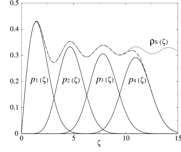
FIG. 1.: Microscopic spectral density $\rho_{S}(\zeta)$ (thin line), $k$-th smallest eigenvalue distribution $p_{k}(\zeta)$, $k=1,2,3,4$ (solid lines), and their sum $\sum_{k=1}^{4}p_{k}(\zeta)$ (broken line) for the quenched chiral unitary ensemble ($\beta=2,N_{f}=\nu=0$).

REFERENCES

- [1] H. Leutwyler and A. Smilga, Phys. Rev. D46, 5607 (1992).
- [2] A. Smilga and J.J.M. Verbaarschot, Phys. Rev. D51, 829 (1995).
- [3] E.V. Shuryak and J.J.M. Verbaarschot, Nucl. Phys. A560, 306 (1993).
-
[4]
J.J.M. Verbaarschot and I. Zahed,
Phys. Rev. Lett. 70, 3852 (1993);
J.J.M. Verbaarschot, Nucl. Phys. B426 (1994) 559; Phys. Rev. Lett. 72, 2531 (1994). - [5] M.A. Halasz and J.J.M. Verbaarschot, Phys. Rev. D52, 2563 (1995).
- [6] For an exhaustive list of references, see: J.J.M. Verbaarschot and T. Wettig, hep-ph/0003017.
-
[7]
P.H. Damgaard, Phys. Lett. B424, 322 (1998).
G. Akemann and P.H. Damgaard, Nucl. Phys. B528, 411 (1998); Phys. Lett. B432, 390 (1998); hep-th/9910190. -
[8]
J.C. Osborn, D. Toublan and J.J.M. Verbaarschot,
Nucl. Phys.
B540, 317 (1999);
P.H. Damgaard, J.C. Osborn, D. Toublan and J.J.M. Verbaarschot, Nucl. Phys. B547, 305 (1999);
D. Toublan and J.J.M. Verbaarschot, Nucl. Phys. B560, 259 (1999). - [9] T. Nagao and K. Slevin, J. Math. Phys. 34, 2075 (1993).
- [10] P.J. Forrester, Nucl. Phys. B402, 709 (1993).
- [11] P.J. Forrester, J. Math. Phys. 35, 2539 (1994).
- [12] A.V. Andreev, B.D. Simons, and N. Taniguchi, Nucl. Phys. B432, 487 (1994).
- [13] T. Nagao and P.J. Forrester, Nucl. Phys. B435, 401 (1995).
- [14] P.H. Damgaard and S.M. Nishigaki, Nucl. Phys. B518, 495 (1998).
- [15] T. Wilke, T. Guhr, and T. Wettig, Phys. Rev. D57, 6486 (1998).
- [16] T. Nagao and S.M. Nishigaki, hep-th/0001137, Phys. Rev. D62 (2000) in press.
- [17] G. Akemann and E. Kanzieper, hep-th/0001188.
- [18] T. Nagao and S.M. Nishigaki, hep-th/0003009, Phys. Rev. D62 (2000) in press.
- [19] K. Slevin and T. Nagao, Phys. Rev. Lett. 70, 635 (1993).
- [20] C.A. Tracy and H. Widom, Commun. Math. Phys. 161, 289 (1994).
- [21] P.J. Forrester and T.D. Hughes, J. Math. Phys. 35, 6736 (1994).
- [22] T. Nagao and P.J. Forrester, Nucl. Phys. B509, 561 (1998).
- [23] S.M. Nishigaki, P.H. Damgaard, and T. Wettig, Phys. Rev. D58, 087704 (1998).
-
[24]
S. Nishigaki, Phys. Lett. B387, 139 (1996);
G. Akemann, P.H. Damgaard, U. Magnea, and S. Nishigaki, Nucl. Phys. B487, 721 (1997). - [25] E. Kanzieper and V. Freilikher, Philos. Mag. B77, 1161 (1998).
-
[26]
M.K. Şener and J.J.M. Verbaarschot, Phys. Rev. Lett. 81,
248 (1998).
B. Klein and J.J.M. Verbaarschot, hep-th/0004119. - [27] H. Widom, J. Stat. Phys. 94, 347 (1999).
-
[28]
R. Brower, P. Rossi, and C.-I. Tan, Nucl. Phys. B190,
699 (1981).
A.D. Jackson, M.K. Şener, and J.J.M. Verbaarschot, Phys. Lett. B387, 355 (1996). - [29] M.L. Mehta, Random Matrices, 2nd Ed. (Academic, San Diego, 1991).
- [30] C.A. Tracy and H. Widom, Springer Lecture Note in Physics 424, 103 (1993).