hep-th/0006099

MZ-TH/00-25

Rotation Symmetry Breaking Condensate
in a Scalar Theory

O. Lauscher

M. Reuter

Institut für Physik, Universität Mainz
Staudingerweg 7, 55099 Mainz, Germany

C. Wetterich

Institut für Theoretische Physik, Universität Heidelberg
Philosophenweg 16, 69120 Heidelberg, Germany

Motivated by an analogy with the conformal factor problem in gravitational theories of the $R+R^{2}$-type we investigate a $d$-dimensional Euclidean field theory containing a complex scalar field with a quartic self interaction and with a nonstandard inverse propagator of the form $-p^{2}+p^{4}$. Nonconstant spin-wave configurations minimize the classical action and spontaneously break the rotation symmetry to a lower-dimensional one. In classical statistical physics this corresponds to a spontaneous formation of layers. Within the effective average action approach we determine the renormalization group flow of the dressed inverse propagator and of a family of generalized effective potentials for nonzero-momentum modes. Already in the leading order of the semiclassical expansion we find strong “instability induced” renormalization effects which are due to the fact that the naive vacuum (vanishing field) is unstable towards the condensation of modes with a nonzero momentum. We argue that the (quantum) ground state of our scalar model indeed leads to spontaneous breaking of rotation symmetry.

I Introduction

It is a common feature of several Euclidean field theories of physical interest that spatially inhomogeneous, i.e. nonconstant field configurations have a lower value of the action functional than homogeneous ones. This means that, at least semiclassically, the inhomogeneous configurations are likely to dominate the functional integral and thus to determine the quantum vacuum state $\left|0\right>$. In this case we expect that the essential features of the true vacuum state can be understood by an expansion in the quantum fluctuations about a set of configurations with a position-dependent, non-translational invariant value of the field variable. In the quantum vacuum this “condensation” of spatially inhomogeneous modes contributes to certain expectation values $\left<0\right|{\cal O}\left|0\right>\neq 0$ where ${\cal O}$ is a scalar operator constructed from the derivatives of the fundamental fields in such a way that it is sensitive to the nonvanishing kinetic energy of the contributing configurations. (For instance, in a scalar model, ${\cal O}=\partial_{\mu}\phi\,\partial^{\mu}\phi$.) We shall generically refer to such contributions as “kinetic condensates”. They are to be distinguished from the familiar translational invariant “potential condensates” characterizing the conventional Higgs mechanism which is triggered by a nonzero but constant scalar field expectation value.

In this context one should distinguish two different physical situations. If the degenerate minimum of the effective action corresponds to configurations which are not invariant under some global symmetry like translations or rotations such a symmetry is spontaneously broken and only the remaining unbroken symmetry can be used for a classification of the spectrum of excitations. This spectrum will typically contain massless “Goldstone-excitations”. In this case one typically has an order parameter whose expectation value breaks the symmetry, in addition to the invariant kinetic operators mentioned above. In the second case the dominant configurations break a local symmetry. Then it is well known that there is no true spontaneous symmetry breaking and no nonzero expectation value of a noninvariant order operator exists. Also the “Goldstone-excitations” are absent from the physical spectrum. Nevertheless, we have learned from the Higgs-mechanism in the electroweak standard model that a language in terms of “spontaneous symmetry breaking” can be very useful. This spontaneous symmetry breaking manifests itself in nonperturbative contributions to invariant operators for “kinetic condensates”.

A typical example of a kinetic condensate is the gluon condensate in QCD. While the classical Yang-Mills action $1/4\int d^{4}xF_{\mu\nu}^{a}F_{\mu\nu}^{a}$ is minimized by $F_{\mu\nu}=0$, already the one-loop effective action assumes its minimum for $F_{\mu\nu}\neq 0$. The Savvidy vacuum [1] tries to model the true ground state as a covariantly constant color magnetic field. The effective action of this state is indeed lower than that for $F_{\mu\nu}=0$. It is known, however, that the Savvidy vacuum is unstable in the infrared (IR), and it has been speculated that the dominant configurations may be spatially inhomogeneous (perhaps domain-like) in order to provide an IR cutoff at a scale set by $\Lambda^{-1}_{\rm QCD}$. Those nontrivial properties of the QCD vacuum are parametrized by $\left<0\right|F_{\mu\nu}^{a}F_{\mu\nu}^{a}\left|0\right>$ and similar condensates of more complicated gauge- and Lorentz-invariant operators.

Another important example is Euclidean gravity based upon the Einstein-Hilbert action [2]

$$S_{\rm EH}\left[g_{\mu\nu}\right]=-\frac{1}{16\pi G}\int d^{4}x\,\sqrt{g}\,R$$ (1)

which is not positive definite. In fact, decomposing the metric as $g_{\mu\nu}=\exp(2\phi)\bar{g}_{\mu\nu}$ where $\bar{g}_{\mu\nu}$ is a fixed reference metric, we obtain

$$S_{\rm EH}\left[g_{\mu\nu}\right]=-\frac{1}{16\pi G}\int d^{4}x\,\sqrt{\bar{g}}\,e^{2\phi}\,\left[\bar{R}+6\,\bar{g}^{\mu\nu}\,\bar{D}_{\mu}\phi\,\bar{D}_{\nu}\phi\right]\,.$$ (2)

This shows that $S_{\rm EH}$ can become arbitrarily negative if the conformal factor $\phi(x)$ varies rapidly enough so that $(\bar{D}_{\mu}\phi)^{2}$ is large. Leaving aside for a moment the well known problems in setting up a consistent theory of quantum gravity, it is tempting to speculate that the theory cures this instability caused by the unboundedness of $S_{\rm EH}$ in a dynamical way. Nonconstant $\phi$-modes could condense in such a way that the resulting quantum vacuum state is stable and constitutes the absolute minimum of some yet unknown effective action functional. The expectation value of the metric in this state should be close to the metric for flat space (which is not the minimum of $S_{\rm EH}$!). Also, operators like $(\bar{D}_{\mu}\phi)^{2}$, appropriately covariantized, should acquire nonzero expectation values. This would indicate that the true vacuum arises from a “dynamical stabilization” of the bare theory due to the condensation of nonconstant $\phi$-modes.

A further model in which the existence of a variant of the “kinetic condensate” has been speculated about is Liouville field theory [3], [4]. The expectation value of its operatorial equation of motion reads

$$\left<0\left|\Box\phi\right|0\right>+\frac{m^{2}}{\beta}\,\left<0\left|e^{\beta\phi}\right|0\right>=0\,.$$ (3)

Provided it is possible to make the operator $\exp(\beta\phi)$ well defined and that the regularized operator is still positive definite, $\rm eq.\,(\ref{i0})$ implies that $\left<0\left|\Box\phi\right|0\right>$ is nonzero and, as a consequence, that the vacuum $\left|0\right>$ is not translational invariant.

In the examples mentioned above the determination of the vacuum state is a formidable task which has not been mastered yet. In the present paper we shall therefore study the formation of a “kinetic condensate” within the framework of a scalar toy model. On the one hand, this model is simple enough to be treated analytically, on the other hand it is found to have the feature of a “dynamical stabilization” which we hope to occur in QCD and in quantum gravity.

The model is formulated in $d$ Euclidean dimensions. It contains a massless complex scalar field $\chi$ with a conventional $\lambda|\chi|^{4}$-self interaction but with a higher-derivative kinetic term:

$$S\left[\chi\right]=\int d^{d}x\,\left\{\chi^{*}\,\Omega(-\Box)\,\chi+\frac{\lambda}{2}\,|\chi|^{4}\right\}$$ (4)

The kinetic operator $\Omega$ is taken to be

$$\Omega(-\Box)=\Box+\frac{\Box^{2}}{2M^{2}}\;,\;\;\Box=\partial_{\mu}\partial_{\mu}\;,$$ (5)

so that in momentum space

$$\Omega(p^{2})=-p^{2}+\frac{(p^{2})^{2}}{2M^{2}}$$ (6)

where $M$ is a constant with the dimension of a mass. On a Euclidean spacetime where $p^{2}\equiv p_{\mu}p_{\mu}\geq 0$, the kinetic operator is positive for $p^{2}>2M^{2}$ but negative for momenta between $p^{2}=0$ and $p^{2}=2M^{2}$. It has a minimum at $p^{2}=M^{2}$ where it assumes the value $-M^{2}/2$, see FIG. 1. The action (4) has a global U(1)-invariance under phase rotations $\chi\rightarrow\chi\,\exp(i\varphi)$ with a constant $\varphi$, and it is invariant under the Euclidean Poincaré group ISO($d$) of rigid spacetime translations and rotations.

We will see that in this model the rotation symmetry is spontaneously broken whereas a modified translation symmetry is preserved. As a classical statistical system in $d=3$ dimensions or the (zero temperature) ground state of a quantum statistical system ($d=4$) this models the spontaneous formation of two-dimensional layers which break the rotation symmetry. An effective translation symmetry rotates the phase factor of the complex field $\phi$ by $2\pi$ as one translates from one layer to the next. In two dimensions it corresponds to the spontaneous generation of line-like structures. We emphasize that the microscopic action has rotation and translation symmetry, in contrast to lattice models. Our model therefore describes situations where already a tiny perturbation of these symmetries results in nontrivial geometric structures.

The model shares some essential features with the conformal sector of a gravitational model of the type $S[g_{\mu\nu}]=\int d^{d}x\,\sqrt{g}\{\alpha\,R+\beta\,R^{2}\}$, for instance. (Here “$R^{2}$” stands for any invariant quadratic in the Riemann tensor.) The Euclidean classical action of this model is bounded below, in contrast to the Einstein-Hilbert action. It is therefore a good starting point for the definition of a Euclidean functional integral if the problems of UV regularization can be mastered. The Einstein-Hilbert term $\sqrt{g}R$ leads to a negative contribution to the kinetic term of the conformal factor of the metric, which dominates at small momenta, while the $R^{2}$-term gives rise to a positive contribution dominating at large momenta. The instability at small and the stability at large momenta is modelled by the ansatz (6) with $M$ playing the role of the Planck mass.

The “wrong sign” $p^{2}$-term in (6) induces an instability of the naive vacuum with $\chi=0$ towards the formation of a spatially inhomogeneous ground state because the system tends to lower its Euclidean action by making the kinetic action $\int_{p}\Omega(p^{2})|\tilde{\chi}(p)|^{2}$ as negative as possible. Thus we expect that the vacuum of this model is dominated by nonconstant field configurations whose typical momenta are of the order of the scale $M$. We shall see that this is actually the case.

The true vacuum configuration $\left<\chi(x)\right>$ of any theory can be found from its (standard) effective action $\Gamma[\phi]$ by solving the “dressed” field equation $\delta\Gamma/\delta\phi=0$. In this paper we consider $\Gamma$ as the zero-cutoff limit of the effective average action $\Gamma_{k}[\phi]$, a type of coarse grained free energy with a variable infrared (IR) cutoff at the mass scale $k$ [5]. It satisfies an exact renormalization group equation, and it interpolates between the classical action $S=\Gamma_{k\rightarrow\infty}$ and the standard effective action $\Gamma=\Gamma_{k\rightarrow 0}$. For our model we shall determine the renormalization group trajectory $k\rightarrow\Gamma_{k}$ in the leading order of the semiclassical expansion which, as we shall argue, provides a qualitatively correct picture already.

The functional $\Gamma_{k}[\phi]$ has the same U(1) and ISO($d$) symmetry as the classical action. In particular, the bilinear term of $\Gamma\equiv\Gamma_{0}$ has the same structure as the one in $S$ but $\Omega(p^{2})$ is replaced by the dressed inverse propagator $\Omega_{\rm eff}(p^{2})$. In FIG. 1 we have plotted our result for $\Omega_{\rm eff}$. Quite remarkably, due to the renormalization effects, the kinetic term has become positive semidefinite even for a vanishing “background field” $\phi$. For all modes with $p^{2}\neq M^{2}$ it “costs” energy (action) to excite them. By including renormalization effects these modes have been stabilized in a dynamical way. On the other hand, modes with $p^{2}=M^{2}$ can be excited “for free”. This indicates that those modes might be unstable towards the formation of a condensate.

FIG. 1.: Classical inverse propagator $\Omega$ and quantum inverse propagator $\Omega_{\rm eff}$ (for zero background field) as functions of ${\rm p}\equiv|p|$.

We shall analyze this phenomenon in terms of a family of generalized momentum dependent effective potentials $U_{k}(A;p^{2})$ which are obtained by evaluating $\Gamma_{k}[\phi]$ for plane-wave arguments $\phi=A\,\exp(ip_{\mu}x_{\mu}+i\beta)$. It turns out that for $k\rightarrow 0$ and $p^{2}\neq M^{2}$ all $U_{k}$’s have their minimum at $A=0$ so that the corresponding modes do not acquire a vacuum expectation value. For $p^{2}=M^{2}$ the situation is different: in the limit $k\rightarrow 0$ the potential $U_{k}(A;M^{2})$ develops a flat bottom which signals a nonzero expectation value, i.e. a condensation of the plane-wave modes with momenta $p_{\mu}=Mn_{\mu}$. Here $n_{\mu}$ is an arbitrary unit vector. Indeed, for small but nonzero $k$ the absolute minimum of $\Gamma_{k}$ occurs (within our approximation) for $A\neq 0$ in the mode $p^{2}=M^{2}$.

In leading order we find the following expectation value of the fundamental field:

$$\left<\chi(x)\right>=\frac{M}{\sqrt{2\lambda}}\,\exp\left(iMn_{\mu}x_{\mu}+i\alpha\right)$$ (7)

It is characterized by the phase $\alpha$ and the vector $n_{\mu}$. This means that the above expectation value leads to a spontaneous breaking of both the U(1) and the ISO($d$) symmetry. For the translations in the directions $n_{\mu}$ only a remaining symmetry corresponding to combined transformations of the form

$$x^{\prime}_{\mu} = x_{\mu}+\frac{\xi}{M}\,n_{\mu}$$ (8)

$$\alpha^{\prime} = \alpha-\xi$$ (9)

is left unbroken, where $\xi$ represents a real, constant parameter. For such combined transformations the symmetry breaking from the spacetime translations is compensated by an appropriate phase rotation so that $Mn_{\mu}x_{\mu}+\alpha=Mn_{\mu}x_{\mu}^{\prime}+\alpha^{\prime}$. The case $\xi=2\pi m$, $m$ integer, is special in the sense that no compensating phase rotation is needed to achieve invariance. Therefore we obtain a symmetry with respect to discrete spacetime translations given by

$$x^{\prime}_{\mu} = x_{\mu}+\frac{2\pi m}{M}\,n_{\mu}\,.$$ (10)

As was already mentioned above the spontaneous breaking of the ISO($d$) symmetry to this discrete symmetry is analogous to the spontaneous formation of layers in statistical systems where the transformation (10) describes a translation from one layer to another. We emphasize that the layer structure involves the internal degrees of freedom whereas U(1) invariant operators have translationally invariant expectation values due to the combined effective translation symmetry.

By analyzing the spectrum of small fluctuations about the vacuum configuration (7) we find that all those fluctuations are stable. This dynamical stabilization of an apparent tree-level instability is formally analogous to what happens in the familiar situation of an ordinary kinetic term “$+p^{2}$” along with a symmetry breaking potential $V=-\mu^{2}|\chi|^{2}+(\lambda/2)|\chi|^{4}$. In this case the naive vacuum $\chi=0$ is unstable because of the negative mass term, and shifting the field by a constant is sufficient to reach the true vacuum. In our model the analogous “shift to the new vacuum” is more involved since the field variable is shifted by an explicitly $x_{\mu}$-dependent field.

The various candidates for the “vacuum field configuration” can be distinguished by their contribution to the expectation value of $\partial_{\mu}\chi^{*}\partial_{\mu}\chi$. Clearly $\left<\partial_{\mu}\chi^{*}\partial_{\mu}\chi\right>=0$ for the perturbative vacuum, while we find for the ground state (7)

$$\left<\partial_{\mu}\chi^{*}\partial_{\mu}\chi\right>=\frac{M^{4}}{2\lambda}\,.$$ (11)

This is a translational invariant “kinetic condensate” quite analogous to the gluon condensate in QCD. The condensate (11) is nonanalytic in the coupling $\lambda$, i.e. it could not be seen in any finite order of perturbation theory.

The remaining sections of this paper are organized as follows. In section II we discuss the classical vacua, i.e. the degenerate absolute minimum of the functional $S[\chi]$, and we determine the spectrum of small fluctuations about those field configurations. In sections III and IV we review some aspects of the average action approach, and we discuss the phenomenon of “classical renormalization”. It is well known that in theories where standard perturbation theory about the trivial vacuum $\chi=0$ is applicable the lowest order (i.e., classical) approximation of the loop expansion yields $\Gamma=S$ and, more generally, $\Gamma_{k}=S$. We shall see that for unstable theories such as the one investigated here $\Gamma$ does not equal $S$ plus terms induced by loops. There are nontrivial renormalization effects even at the classical level. The reason is that in this case the loop expansion must be performed about the true minimum of the classical action rather than the false vacuum configuration $\chi=0$. Within the loop expansion this type of classical renormalization [6] is refered to as “instability induced” [7] as opposed to the familiar “fluctuation induced” renormalization coming from the loops. In order to understand the full quantum theory at a qualitative level it is often sufficient to take the classical renormalization of the effective action into account. It encodes the physics related to the shift to the true vacuum.

The average action $\Gamma_{k}$ is defined in terms of a functional integral which contains a modified classical action $S_{k}^{J}$ containing the IR-cutoff and source terms. The semiclassical expansion will be applied to this integral. Therefore we need to know the absolute minimum $\chi_{\rm min}(x;J,k)$ of this functional. In section V we derive a sufficient condition for a configuration to be the global minimum of $S_{k}^{J}$. This is used in section VI in order to establish that for vanishing sources the minimum is constituted by spin waves of the type (7). For $J\neq 0$ the situation is more complicated and the corresponding discussion can be found in appendix A.

In section VII we compute the bilinear term of $\Gamma_{k}$ and derive the renormalization group flow of the dressed inverse propagator $\Sigma_{k}(p^{2})$ for vanishing background field. In particular, at the end point $k=0$, we obtain the full quantum inverse propagator $\Omega_{\rm eff}(p^{2})$. In section VIII we identify regions in field space with no classical renormalization, i.e. configurations $\phi$ for which $\Gamma_{k}[\phi]=S[\phi]$ is indeed true in lowest order. Then, in section IX, we combine all pieces of information available in order to draw a global picture of the effective average action $\Gamma_{k}$. We introduce the momentum dependent potentials $U_{k}(A;p^{2})$ and use them to discuss the structure of the true vacuum. Some calculational details are given in the appendices B, C and D. The conclusions are given in section X.

II Spin waves and their fluctuation spectrum

For every Euclidean field theory the field configuration $\chi_{\rm min}$ with the smallest possible value of the action $S$ is of special importance. For a massless $|\chi|^{4}$-theory with an ordinary kinetic term $\Omega=+p^{2}$ this configuration is $\chi_{\rm min}(x)=0$ which puts to zero the potential and the kinetic energy separately. In our case the situation is less trivial because $\Omega(p^{2})$ can assume negative values and hence it is able to compensate for positive contributions coming from the potential. In fact, we shall prove later on in a more general context that the absolute minimum of the action (4) is achieved for the “spin” wave configurations

$$\chi_{\rm min}(x)=\frac{M}{\sqrt{2\lambda}}\,\exp\left(iMn_{\mu}x_{\mu}+i\alpha\right)\,.$$ (12)

Here $n_{\mu}$ is an arbitrary unit vector (a point on $S^{d-1}$) and $\alpha$ is a free phase. Thus the global minimum is degenerate and the corresponding “vacuum manifold” is $S^{1}\times S^{d-1}$. Different points of this manifold correspond to different classical ground states of the theory. If we pick one of those ground states, characterized by a fixed pair $(n,\alpha)$, this amounts to a spontaneous breaking of the ISO($d$) symmetry of spacetime rotations and translations as well as of the U(1) group of global phase transformations.

The classical $(n,\alpha)$-vacua are characterized by a nonzero expectation value of the operator $\partial_{\mu}\chi^{*}\,\partial_{\mu}\chi$, for instance. The spin wave solution (12) yields

$$\left<\partial_{\mu}\chi^{*}\,\partial_{\mu}\chi\right>\equiv\partial_{\mu}\chi_{\rm min}^{*}\,\partial_{\mu}\chi_{\rm min}=\frac{M^{4}}{2\lambda}\,.$$ (13)

In order to further illustrate the physics of this kind of spontaneous symmetry breaking let us look at the spectrum of small fluctuations $\delta\chi$ (particle excitations) about the ground state. Inserting $\chi=\chi_{\rm min}+\delta\chi$ into (4) yields

$$S\left[\chi_{\rm min}+\delta\chi\right]=S\left[\chi_{\rm min}\right]+S_{\rm fluct}\left[\chi_{\rm min},\delta\chi\right]+{\cal O}\left(\delta\chi^{3}\right)$$ (14)

with

$$S_{\rm fluct}\left[\chi_{\rm min},\delta\chi\right]=\frac{1}{2}\int d^{d}x\,\left(\delta\chi^{*},\delta\chi\right)\,\hat{S}^{(2)}[\chi_{\rm min}]\,\left(\begin{array}[]{c}\delta\chi\\ \delta\chi^{*}\end{array}\right)$$ (17)

where $\hat{S}^{(2)}$ is the $2\times 2$ matrix differential operator corresponding to the second functional derivatives of $S$ with respect to $\chi$ and $\chi^{*}$. In appendix B we diagonalize this operator by a linear transformation from $(\delta\chi,\delta\chi^{*})$ to new, real fields $\Phi_{1}$ and $\Phi_{2}$. In terms of the new fields $S_{\rm fluct}$ reads, in momentum representation,

$$S_{\rm fluct}\left[\chi_{\rm min},\delta\chi\right]=\frac{1}{2}\int\frac{d^{d}p}{(2\pi)^{d}}\,\left\{\Phi_{1}(-p)\,{\cal K}_{1}\left(p^{2},\theta\right)\,\Phi_{1}(p)+\Phi_{2}(-p)\,{\cal K}_{2}\left(p^{2},\theta\right)\,\Phi_{2}(p)\right\}$$ (18)

where $\theta$ is the angle between $n_{\mu}$ and $p_{\mu}$. The kinetic terms ${\cal K}_{1/2}$ are given by

$${\cal K}_{1}\left(p^{2},\theta\right) = M^{2}+4\cos^{2}\theta\,p^{2}+\frac{p^{4}}{M^{2}}-\sqrt{M^{4}+16\frac{\cos^{2}\theta}{M^{2}}\,p^{6}}=4\cos^{2}\theta\,p^{2}+{\cal O}(p^{4})$$ (19)

$${\cal K}_{2}\left(p^{2},\theta\right) = M^{2}+4\cos^{2}\theta\,p^{2}+\frac{p^{4}}{M^{2}}+\sqrt{M^{4}+16\frac{\cos^{2}\theta}{M^{2}}\,p^{6}}$$ (20)

$$= 2M^{2}+4\cos^{2}\theta\,p^{2}+{\cal O}(p^{4})=4\cos^{2}\theta\left(\frac{M^{2}}{2\cos^{2}\theta}+p^{2}\right)+{\cal O}(p^{4})\,.$$ (21)

In FIG. 2 we plot ${\cal K}_{1}$ and ${\cal K}_{2}$ for $\theta=0$ and $\theta=\pi/2$ which amounts to excitations propagating parallel and perpendicular to the vacuum direction $n_{\mu}$, respectively. For other values of $\theta$ the behaviour is qualitatively similar.

The mode $\Phi_{1}$ is a massless excitation with an inverse propagator ${\cal K}_{1}$ which vanishes at $p=0$ for any $\theta$. It represents the Goldstone boson of the spontaneously broken global U(1) symmetry. The spontaneous breaking of the SO($d$) rotation symmetry manifests itself in the $\theta$-dependence of the propagator. In particular, one should note that momenta orthogonal to $Q_{0\mu}=Mn_{\mu}$ (i.e. $\cos\theta=0$) correspond to the “Goldstone direction” with ${\cal K}_{1}=p^{4}/M^{2}$. The mode $\Phi_{2}$ is massive for all values of $\theta$. Its direction-dependent mass is given by $M/(\sqrt{2}\cos\theta)$. It is the analogue of the “Higgs” or “radial” mode in the more familiar case of a spontaneous symmetry breaking by a Mexican-hat potential.

(a)

(b)

FIG. 2.: ${\cal K}_{1}$ (lower curve) and ${\cal K}_{2}$ in units of $M^{2}$ as functions of $|p|/M$ plotted for (a) $\theta=0$ and (b) $\theta=\pi/2$.

III The effective average action

Before embarking on the detailed analysis of the theory let us briefly comment on the method we are going to employ. In order to find the true vacuum state we need nonperturbative information about the (conventional) effective action $\Gamma[\phi]$ where $\phi$ is the vacuum expectation value of $\chi$. As we mentioned in the introduction we regard $\Gamma$ as the physical limit of the effective average action $\Gamma_{k}[\phi]$ which was introduced in refs. [5]. The functional $\Gamma_{k}$ results from the classical action $S$ by integrating out only the field modes with momenta larger than the infrared cutoff $k$. Changing $k$ corresponds to a Wilson type renormalization. The conventional effective action $\Gamma$ is recovered in the limit $k\rightarrow 0$. In the space of all actions, the renormalization group trajectory $\Gamma_{k}$, $k\in[0,\infty)$, interpolates between the classical action $S=\Gamma_{k\rightarrow\infty}$ and the standard effective action $\Gamma=\Gamma_{k\rightarrow 0}$. It can be obtained by solving an exact functional renormalization group equation.

The infrared cutoff is implemented by modifying the path integral for the generating functional of the connected Green’s functions according to

$$\exp\left\{W_{k}\left[J\right]\right\} = \int{\cal D}\chi\,\exp\bigg{\{}-S\left[\chi\right]-\int d^{d}x\,\chi^{*}(x)\,{\cal R}_{k}\left(-\Box\right)\,\chi(x)$$ (23)

$$+\int d^{d}x\,\left\{\chi^{*}(x)\,J(x)+J^{*}(x)\,\chi(x)\right\}\bigg{\}}\,.$$

Here ${\cal R}_{k}(p^{2})$ is a to some extent arbitrary positive function which interpolates smoothly between ${\cal R}_{k}(p^{2})\rightarrow k^{2}$ for $p^{2}\rightarrow 0$ and ${\cal R}_{k}(p^{2})\rightarrow 0$ for $p^{2}\rightarrow\infty$. It suppresses the contribution of the small-momentum modes by a mass term $\propto k^{2}$ which acts as the IR cutoff. In practical computations ${\cal R}_{k}(p^{2})=p^{2}\left[\exp\left(p^{2}/k^{2}\right)-1\right]^{-1}$ has been used often. In cases where this does not lead to UV divergences the condition ${\cal R}_{k}(p^{2})\rightarrow 0$ for $p^{2}\rightarrow\infty$ can be relaxed and one may also use a constant cutoff function ${\cal R}_{k}=k^{2}$ which amounts to a momentum independent mass term. For the purposes of our present investigation this simple cutoff will be sufficient.

The Legendre transform of $W_{k}$ reads

$$\widetilde{\Gamma}_{k}\left[\phi\right]=\int d^{d}x\,\left\{\phi^{*}\,J+J^{*}\,\phi\right\}-W_{k}\left[J\right]$$ (24)

where the functional $J=J(\phi)$ is obtained by inverting the relations

$$\phi(x)=\frac{\delta W_{k}}{\delta J^{*}(x)}\;,\;\;\phi^{*}(x)=\frac{\delta W_{k}}{\delta J(x)}$$ (25)

which define the $k$-dependent average field $\phi=\left<\chi\right>$. The effective average action is obtained from (24) by subtracting the cutoff term at the level of the average fields:

$$\Gamma_{k}\left[\phi\right]=\widetilde{\Gamma}_{k}\left[\phi\right]-\int d^{d}x\,\phi^{*}\,{\cal R}_{k}\left(-\Box\right)\,\phi$$ (26)

It can be represented by an implicit functional integral

$$\exp\left\{-\Gamma_{k}\left[\phi\right]\right\} = \int{\cal D}\sigma\,\exp\Bigg{\{}-S[\phi+\sigma]-\int d^{d}x\,\sigma^{*}\,{\cal R}_{k}\,\sigma$$ (28)

$$+\int d^{d}x\,\left(\sigma^{*}\,\frac{\delta\Gamma_{k}}{\delta\phi^{*}}[\phi]+\sigma\,\frac{\delta\Gamma_{k}}{\delta\phi}[\phi]\right)\Bigg{\}}\,.$$

Here we introduced the shifted field

$$\sigma\equiv\chi-\phi\,.$$ (29)

It has been shown [5] that the functional defined in this way has the interpolating properties stated above, and that it satisfies an exact renormalization group equation. In the present paper we shall not use this flow equation but rather calculate $\Gamma_{k}$ directly from the above definition. We shall evaluate the path integral (28) or (23) by means of a saddle point approximation. It will turn out that the global minimum of the Euclidean action can be found analytically. By expanding about this minimum and properly taking its degeneracies into account we will be able to deduce the essential features of the true vacuum already from the lowest order of the saddle point approximation. In the following we shall disregard loop effects. Because of the nontrivial vacuum structure of the theory, already the “tree-level” approximation yields nontrivial renormalization effects.

For configurations $\phi_{\rm sw}$ close to the spin wave solution (7) the saddle point approximation for the effective average action obeys for all $k$

$$\Gamma_{k}\left[\phi_{\rm sw}\right]=S\left[\phi_{\rm sw}\right]\,.$$ (30)

This follows directly from (28) by an expansion of $\phi_{\rm sw}$ around (7) and an expansion in powers of $\sigma$. The terms linear in $\sigma$ cancel and the term quadratic in $\sigma$ is positive by virtue of the discussion in the last section. If the solution (7) corresponds to the absolute minimum of $\Gamma_{k}$ for small positive $k$ the rotation symmetry is spontaneously broken. Indeed, if one adds a small source term $J(\vec{q})$ the degeneracy of the minimum is lifted and the absolute minimum will occur for the same momentum direction and the same phase as $J$. In the limit $J\rightarrow 0$ the spin-wave configuration and its orientation persist - this is spontaneous symmetry breaking. We will see below that this spontaneous symmetry breaking of rotation symmetry is indeed realized for our scalar model.

IV Effective average action near the origin and classical renormalization effects

In order to establish that the spin-wave configuration (7) corresponds to the absolute minimum of $\Gamma_{k}$ for small positive $k$ we need to understand the behaviour of $\Gamma_{k}$ for arbitrary $\phi$. In this section we concentrate on small values of $\phi$, i.e. configurations that are far away from the spin-wave solution. In particular, we want to understand the issue of convexity of the effective action for $k\rightarrow 0$ in case of spontaneous breaking of rotation symmetry.

We are interested in the expansion of $\Gamma_{k}$ quadratic in $\phi$, i.e. the two-point function at the origin. For this purpose we exploit the fact that the origin $\phi=0$ always corresponds to a stationary point of $\Gamma_{k}$ by virtue of the symmetries. By continuity we infer that - except for the phase with spontaneous symmetry breaking - small values of $\phi$ correspond to small sources $J$. In this case we will directly evaluate the scale dependent generating functional $W_{k}$ for the theory (4) which is given by the path integral

$$\exp\left\{W_{k}\left[J\right]\right\}=\int{\cal D}\chi\,\exp\left\{-S_{k}^{J}[\chi;J]\right\}$$ (31)

with

$$S_{k}^{J}[\chi;J] = S_{k}\left[\chi\right]-\int d^{d}x\,\left\{J^{*}\,\chi+J\,\chi^{*}\right\}$$ (32)

and

$$S_{k}\left[\chi\right]=\int d^{d}x\,\left\{\chi^{*}\,\omega_{k}(-\Box)\,\chi+\frac{\lambda}{2}\,|\chi|^{4}\right\}\,.$$ (33)

Here

$$\omega_{k}(-\Box)\equiv\Omega(-\Box)+{\cal R}_{k}(-\Box)$$ (34)

is the complete kinetic operator. In momentum space it reads

$$\omega_{k}(p^{2})=-p^{2}+{\cal R}_{k}(p^{2})+\frac{(p^{2})^{2}}{2M^{2}}\;.$$ (35)

For values of the cutoff $k$ which are larger than some critical value $k_{\rm cr}$ the modified inverse propagator $\omega_{k}(p^{2})$ is positive for any value of the momentum $p$ since the regulator term ${\cal R}_{k}(p^{2})$ overrides any negative contribution which could come from $\Omega(p^{2})$. Every admissible function ${\cal R}_{k}(p^{2})$ leads to a $k_{\rm cr}$ which equals $M$ times a number of order unity. The mass-type cutoff ${\cal R}_{k}=k^{2}$ yields $k_{\rm cr}=M/\sqrt{2}$, for instance. As a consequence, for large values of $k$, and in particular for $k$ close to the UV cutoff $\Lambda$ where we start the renormalization group evolution, there is no instability. As we lower the cutoff $k$ below the critical value, $\omega_{k}(p^{2})$ becomes negative for certain modes. Obviously the modes with momenta in a band centered at $p^{2}=M^{2}$ become unstable first. Finally, at $k=0$, all modes with $p^{2}$ in the interval $(0,2M^{2})$ have become unstable in the sense that by exciting such modes we can push the value of the Euclidean action below its value for the trivial configuration $\chi(x)=0$. We suspect that this instability causes the modes with typical momenta of the order of $M$ to “condense”, and it is this phenomenon which we are going to investigate.

The functionals $W_{k}[J]$ and $\Gamma_{k}[\phi]$ enjoy the same invariance properties as the classical action. In addition to Poincaré symmetry they are invariant under $J\rightarrow J\exp(i\varphi)$ and $\phi\rightarrow\phi\exp(i\varphi)$, respectively. This implies that the series expansion of $W_{k}$ in powers of the sources, provided that it exists, contains only terms with an equal number of $J$ and $J^{*}$. In particular, the quadratic term displaying the effective propagator reads

$$W_{k}^{\rm quad}\left[J\right]=\int d^{d}x\,d^{d}y\,J^{*}(x)\,G_{k}(x,y)\,J(y)\equiv\int d^{d}x\,J^{*}(x)\,G_{k}(-\Box)\,J(x)$$ (36)

so that

$$W_{k}\left[J\right]=W_{k}\left[0\right]+W_{k}^{\rm quad}\left[J\right]+\ldots$$ (37)

where the dots stand for terms of order $J^{2}{J^{*}}^{2}$. Likewise, Legendre-transforming (36) and using (26) leads to

$$\Gamma_{k}\left[\phi\right]=-W_{k}\left[0\right]+\Gamma_{k}^{\rm quad}\left[\phi\right]+{\cal O}\left(\phi^{2}\,\phi^{*2}\right)$$ (38)

where

$$\Gamma_{k}^{\rm quad}\left[\phi\right]=\int d^{d}x\,d^{d}y\,\phi^{*}(x)\,\Sigma_{k}(x,y)\,\phi(y)\equiv\int d^{d}x\,\phi^{*}(x)\,\Sigma_{k}(-\Box)\,\phi(x)$$ (39)

with

$$\Sigma_{k}(-\Box)=G_{k}(-\Box)^{-1}-{\cal R}_{k}(-\Box)\;.$$ (40)

Henceforth we interpret $\Sigma_{k}$ as the differential operator $\Sigma_{k}(-\Box)$ or as the function $\Sigma_{k}(p^{2})$ in momentum space.

Frequently we shall evaluate the effective average action for plane-wave configurations $\phi(x)=A\,\exp(ip_{\mu}x_{\mu}+i\alpha)$. Then U(1)-invariance leads to

$$\Gamma_{k}[A\,\exp(ip_{\mu}x_{\mu}+i\alpha)]\equiv{\cal V}\,U_{k}(A;p^{2})\;\;\;\;\;\left({\cal V}\equiv\int d^{d}x\right)$$ (41)

where we refer to $U_{k}(A;p^{2})$ as the effective potential for the mode with momentum $p$. Note that while $\Gamma_{k}$ gives rise to an infinity of such “effective potentials”, one for each momentum, it is clear that the totality of all those potentials contains much less information than $\Gamma_{k}$ since the correlations between different momentum modes are not specified.

In the subsequent sections we evaluate the functional integral (31) by means of a saddle point approximation and determine $\Gamma_{k}$ directly from its definition (24)-(26) rather than by solving a flow equation. Denoting the global minimum of $S_{k}^{J}$ by $\chi_{\rm min}(J)$ the lowest order approximation reads

$$W_{k}\left[J\right]``=\mbox{''}-S_{k}^{J}\left[\chi_{\rm min}(J);J\right]\,.$$ (42)

Under certain conditions (for instance for $J=0$ and $k$ sufficiently small) the global minimum is degenerate. In this case eq. (42) is only symbolic (indicated by the equality sign “=”) and one should sum over the degenerate minima. We ignore this subtlety for a moment.

We shall see that already the lowest order approximation (42) encapsulates all the essential physics which leads to a dynamical stabilization. At first sight this might seem surprising because one could suspect that (42) leads to the trivial result $\Gamma_{k}=S$. In fact, if one performs a conventional perturbative loop expansion in a theory with a positive definite Hessian $S^{(2)}\equiv\delta^{2}S/\delta\chi\,\delta\chi^{*}$ one has the standard lowest-order results $\Gamma=S$ and $\chi_{\rm min}=\phi$. Since all contributions from fluctuations (one-loop determinant etc.) are neglected in (42) one might wonder how, nevertheless, nontrivial renormalization effects can occur.

This point can be understood by looking at the integro-differential equation for $\Gamma_{k}$ given by eq. (28). Now we try to find the ($k$-dependent) global minimum $\sigma_{\rm min}\equiv\sigma_{\rm min}(\phi)$ of the complete action in the exponential of (28). It satisfies

$$\frac{\delta S}{\delta\phi^{*}}\left[\phi+\sigma_{\rm min}\right]+{\cal R}_{k}\,\sigma_{\rm min}=\frac{\delta\Gamma_{k}}{\delta\phi^{*}}\left[\phi\right]\;.$$ (43)

For very large values of $k$, the term $\int d^{d}x\;\sigma^{*}{\cal R}_{k}\sigma$ in (28) strongly suppresses fluctuations with $\sigma\neq 0$, so the main contributions to the integral (28) will come from small oscillations about $\sigma_{\rm min}=0$, which is indeed the global minimum in this case. In this case one has $\chi_{\rm min}\equiv\sigma_{\rm min}+\phi=\phi$ and (43) is obeyed for $\Gamma_{k}=S$. When we lower $k$ towards zero it often happens that $\sigma_{\rm min}=0$ continues to be the absolute minimum of the action. This is the case for classically stable theories with a positive definite Hessian $S^{(2)}$ where no condensation phenomena occur.

On the other hand, eq. (43) may admit also nontrivial solutions with $\sigma_{\rm min}\neq 0$ for $k$ small enough. They are relevant in the case of instabilities where the Hessian $S^{(2)}[\phi]$ develops negative eigenvalues. Setting $\sigma=\sigma_{\rm min}+\psi$ and expanding up to second order in $\psi$ one has, with $\chi_{\rm min}\equiv\phi+\sigma_{\rm min}$,

$$\exp\left\{-\Gamma_{k}\left[\phi\right]\right\} = \exp\Bigg{\{}-S\left[\chi_{\rm min}\right]-\int d^{d}x\,\sigma_{\rm min}^{*}\,{\cal R}_{k}\,\sigma_{\rm min}$$ (46)

$$+\int d^{d}x\,\left(\sigma_{\rm min}^{*}\,\frac{\delta\Gamma_{k}}{\delta\phi^{*}}\left[\phi\right]+\sigma_{\rm min}\,\frac{\delta\Gamma_{k}}{\delta\phi}\left[\phi\right]\right)\Bigg{\}}$$

$$\times\int{\cal D}\psi\,\exp\left\{-\int d^{d}x\,\psi^{*}\left(S^{(2)}\left[\chi_{\rm min}\right]+{\cal R}_{k}\right)\psi\right\}\,.$$

For the “correct” saddle point $S^{(2)}[\chi_{\rm min}]+{\cal R}_{k}$ should be positive semidefinite. The zero modes in case of degeneracy of the minimum lead to an integration over the vacuum manifold. In lowest order one neglects the remaining Gauss integral involving the positive eigenvalues of $S^{(2)}[\chi_{\rm min}]$ and finds

$$\Gamma_{k}\left[\phi\right] ``=\mbox{''} S\left[\chi_{\rm min}\right]+\int d^{d}x\,\sigma_{\rm min}^{*}\,{\cal R}_{k}\,\sigma_{\rm min}-\int d^{d}x\,\left(\sigma_{\rm min}^{*}\,\frac{\delta\Gamma_{k}}{\delta\phi^{*}}\left[\phi\right]+\sigma_{\rm min}\,\frac{\delta\Gamma_{k}}{\delta\phi}\left[\phi\right]\right)$$ (47)

For $\sigma_{\rm min}\neq 0$ (i.e. if $\chi_{\rm min}\neq\phi$) this is still a complicated differential equation for $\Gamma_{k}$ whose solution is not given by $\Gamma_{k}=S$. Hence the lowest order (classical) term of the saddle point approximation does indeed give rise to nontrivial renormalization effects leading to $\Gamma_{k}\neq S$. In fact, all the qualitative features of the condensation phenomena we are interested in are described by this classical term alone. The higher order corrections yield minor quantitative corrections only. For this to be the case it is important to correctly identify the absolute minimum $\chi_{\rm min}$ of the (total) action. At next-to-leading order the fluctuations $\psi$ modify the r.h.s. of (47) by a one-loop term $\ln{\rm Det}^{\prime}\left(S^{(2)}[\chi_{\rm min}]+{\cal R}_{k}\right)$ where the prime at the determinant indicates that the zero modes of $S^{(2)}[\chi_{\rm min}]$ are excluded. For our case of interest this correction is typically small, at least for $d>2$.

In ref. [6] this formalism has been applied to the familiar spontaneous symmetry breaking by a Mexican-hat potential. It was found that the classical term of the saddle point expansion describes all salient features of the effective potential such as the approach of convexity for $k\rightarrow 0$, and that the one-loop determinant does not modify its qualitative properties. In ref. [7] similar classical instability driven renormalization effects have been found in the framework of the Wegner-Houghton equation. For an investigation of a different scalar theory with a higher derivative kinetic term containing the usual positive quadratic kinetic term see ref. [9].

V A sufficient condition for the absolute minimum

Later on we shall use the saddle point approximation to calculate the effective average action. This requires the knowledge of the absolute minimum of the action $S_{k}^{J}$ (32). In order to identify the absolute minimum, we use a method similar to the one outlined in [6]. First we split the field $\chi$ into a classical solution that minimizes the action and an arbitrary, not necessarily small deformation $\delta\chi$:

$$\chi(x)=\chi_{\rm min}(x)+\delta\chi(x)$$ (48)

If we insert this ansatz into the action (32) and take advantage of the fact that $\chi_{\rm min}$ is a solution of the equation of motion (e.o.m.)

$$\frac{\delta S_{k}^{J}}{\delta\chi^{*}} = 0\Leftrightarrow\left[\Omega(-\Box)+{\cal R}_{k}(-\Box)+\lambda\,\left|\chi\right|^{2}\right]\chi=J$$ (49)

we obtain

$$S_{k}^{J}\left[\chi;J\right]=S^{J}_{k}\left[\chi_{\rm min};J\right]+\Delta S_{k}\left[\chi_{\rm min},\delta\chi\right]$$ (50)

where $\Delta S_{k}$ is defined as

$$\Delta S_{k}\left[\chi_{\rm min},\delta\chi\right]\equiv\int d^{d}x\,\bigg{\{}\delta\chi^{*}\left[\Omega(-\Box)+{\cal R}_{k}(-\Box)\right]\delta\chi+\frac{\lambda}{2}\bigg{[}\chi_{\rm min}^{2}\,\left(\delta\chi^{*}\right)^{2}$$ (52)

$$+{\chi_{\rm min}^{*}}^{2}\,\left(\delta\chi\right)^{2}+4\left|\chi_{\rm min}\right|^{2}\,\left|\delta\chi\right|^{2}+2\chi_{\rm min}\,\delta\chi^{*}\,\left|\delta\chi\right|^{2}+2\chi_{\rm min}^{*}\,\delta\chi\,\left|\delta\chi\right|^{2}+\left|\delta\chi\right|^{4}\bigg{]}\bigg{\}}\,.$$

One can read off immediately that a solution of the e.o.m. corresponds to the absolute minimum of $S_{k}^{J}$ if

$$\Delta S_{k}\left[\chi_{\rm min},\delta\chi\right]\geq 0$$ (53)

is satisfied for any deformation $\delta\chi$. Because $\Delta S_{k}$ does not explicitly contain the sources this condition is the same for $S^{J}_{k}$ and $S^{J=0}_{k}=S_{k}$.

It is useful to rewrite the expression for $\Delta S_{k}$ in the following manner.

$$\Delta S_{k}\left[\chi_{\rm min},\delta\chi\right] = \int d^{d}x\,\delta\chi^{*}\left[\Omega(-\Box)+{\cal R}_{k}(-\Box)+\lambda\,\left|\chi_{\rm min}\right|^{2}\right]\delta\chi$$ (55)

$$+\frac{\lambda}{2}\int d^{d}x\,\left(\chi_{\rm min}\,\delta\chi^{*}+\chi_{\rm min}^{*}\,\delta\chi+\left|\delta\chi\right|^{2}\right)^{2}$$

Because $\chi_{\rm min}\,\delta\chi^{*}+\chi_{\rm min}^{*}\,\delta\chi=2{\rm Re}\left(\chi_{\rm min}\,\delta\chi^{*}\right)$ is real the integrand of the second integral in eq. (55) cannot become negative. Therefore we may conclude that

$$\int d^{d}x\,\delta\chi^{*}\left[\Omega(-\Box)+{\cal R}_{k}(-\Box)+\lambda\,\left|\chi_{\rm min}\right|^{2}\right]\delta\chi\geq 0$$ (56)

for any $\delta\chi(x)$ is a sufficient condition for $\chi_{\rm min}$ being the absolute minimum of the action $S_{k}^{J}$ for some suitable source $J$ given by the solution of eq. (49).

VI Searching for the absolute minimum

The aim of this section is to find the field configuration that minimizes the action $S_{k}^{J}$ globally. Here we start with the case of vanishing external sources and relegate the case $J\neq 0$ to appendix A 1. From now on we use the mass-type cutoff function ${\cal R}_{k}=k^{2}$. It simplifies the algebra and allows for particularly transparent results.

We are searching for the minimum of $S_{k}$, so we have to solve the e.o.m.

$$\left[\omega_{k}(-\Box)+\lambda\,\left|\chi\right|^{2}\right]\chi=0\;,\;\;\omega_{k}\equiv\Omega+k^{2}=\Box+\frac{\Box^{2}}{2M^{2}}+k^{2}\;.$$ (57)

Its most obvious solution is the one of vanishing $\chi$, $\chi_{\rm min}=0$. We can now employ the tool we developed in the last section to find out whether $\chi_{\rm min}=0$ constitutes the global minimum. First we insert this solution into eq. (55) which yields

$$\Delta S_{k}\left[\chi=0,\delta\chi\right]=\int d^{d}x\,\delta\chi^{*}\left[\Omega(-\Box)+k^{2}\right]\delta\chi+\frac{\lambda}{2}\int d^{d}x\,\left|\delta\chi\right|^{4}\,.$$ (58)

The next step is to use the Fourier representation

$$\delta\chi(x)=\int\frac{d^{d}p}{(2\pi)^{d}}\,\widetilde{\delta\chi}(p)\,\exp\left(ip_{\mu}x_{\mu}\right)$$ (59)

and to go over to momentum space for the first term:

$$\Delta S_{k}\left[\chi=0,\delta\chi\right]=\int\frac{d^{d}p}{(2\pi)^{d}}\,\left|\widetilde{\delta\chi}(p)\right|^{2}\,\left[\Omega(p^{2})+k^{2}\right]+\frac{\lambda}{2}\int d^{d}x\,\left|\delta\chi\right|^{4}$$ (60)

For $k^{2}\geq M^{2}/2$ one finds that $\omega_{k}(p^{2})=\Omega(p^{2})+k^{2}\geq 0$ and, as a consequence, $\Delta S_{k}$ is always positive (or zero). In this range of $k$ $\chi_{\rm min}=0$ represents the field configuration that minimizes the action globally. However, if $k^{2}<M^{2}/2$, then, for certain deformations with a sufficiently small amplitude, $\Delta S_{k}$ becomes negative. In that case $\chi_{\rm min}=0$ cannot be the absolute minimum.

In order to find the global minimum for $k^{2}<M^{2}/2$ we try the plane wave ansatz

$$\chi_{\rm min}(x)=\chi_{0}\,\exp\left(iQ_{\mu}x_{\mu}+i\alpha\right)\;,\;\;\chi_{0},\,\alpha\;{\rm real}.$$ (61)

Inserting (61) into the e.o.m. leads to the condition

$$\chi_{0}(Q^{2})=\sqrt{-\omega_{k}(Q^{2})/\lambda}\,.$$ (62)

Obviously $\chi_{0}(Q^{2})$ is real only if $\omega_{k}(Q^{2})\leq 0$.

It will be useful to calculate the action for the solution $\chi_{\rm min}$ determined above. We obtain

$$S_{k}\left[\chi=\chi_{0}(Q^{2})\,\exp\left(iQ_{\mu}x_{\mu}+i\alpha\right)\right]=-\frac{{\cal V}}{2\lambda}\,\omega_{k}^{2}(Q^{2})\,.$$ (63)

The action (63) still depends on a free parameter, the momentum squared $Q^{2}$. Hoping to find the absolute minimum for the region of small $k$-values by using the plane wave ansatz, we minimize the expression (63) with respect to $Q^{2}$. This leads to the condition $Q^{2}=M^{2}$. Thus we have found a candidate for the global minimum in the region $k^{2}\leq M^{2}/2$ which is given by

$$\chi_{\rm min}(x)=\hat{\chi}_{0}\,\exp\left(iQ_{0\mu}x_{\mu}+i\alpha\right)\;;\;\;Q_{0\mu}\equiv M\,n_{\mu}\,.$$ (64)

Here $n_{\mu}$ is an arbitrary unit vector ($n^{2}=1$), the phase $\alpha$ is taken to be in $[0,2\pi)$ and

$$\hat{\chi}_{0}\equiv\sqrt{-\frac{1}{\lambda}\omega_{k}(M^{2})}=\sqrt{\frac{1}{\lambda}\left(\frac{1}{2}M^{2}-k^{2}\right)}\;;\;\;k^{2}\leq\frac{1}{2}M^{2}\,.$$ (65)

By inserting the solution (64) into $\Delta S_{k}$ (55) we can check whether it corresponds to the global minimum. In momentum space, the l.h.s. of (56) takes the form

$$\int\frac{d^{d}p}{(2\pi)^{d}}\,\left|\widetilde{\delta\chi}(p)\right|^{2}\,\left[\Omega(p^{2})+\frac{1}{2}M^{2}\right]\,.$$ (66)

Because of $\Omega(p^{2})\geq-M^{2}/2$, this integral is nonnegative and thus the sufficient condition for a global minimum is fulfilled.

Eq. (64) actually describes a whole family of degenerate minima parametrized by the phase $\alpha$ and the unit vector $n_{\mu}$. As a consequence, the “vacuum manifold” is $S^{1}\times S^{d-1}$.

We conclude that the nontrivial solution $(\ref{a25})$ corresponds to the absolute minimum of $S_{k}$ for the region $k^{2}\leq M^{2}/2$, while the solution $\chi_{\rm min}=0$ constitutes the absolute minimum for $k^{2}\geq M^{2}/2$. The two solutions coincide at $k^{2}=M^{2}/2$.

VII Renormalization group flow of the zero field propagator

In this section we compute the scale dependent 2-point function $\Sigma_{k}$ (inverse propagator) which was introduced in eq. (39). The saddle point expansion about the global minimum of $S_{k}^{J}$ leads to

$$\exp\left\{W_{k}\left[J\right]\right\} = N_{k}\,\sum\limits_{\chi_{\rm min}}\exp\bigg{\{}-S_{k}^{J}\left[\chi_{\rm min};J\right]-\frac{1}{2}\,\ln{\rm Det}^{\prime}\hat{S}_{k}^{(2)}\left[\chi_{\rm min}\right]+\ldots\bigg{\}}\,.$$ (67)

Here $\sum_{\chi_{\rm min}}$ denotes a symbolic summation or integration over the possibly degenerate absolute minima. The first term inside the curly brackets of (67) represents the dominant classical term. The second one contains the one-loop effects, and it will be neglected in the following. The normalization constant $N_{k}$ depends on the nature of the minimum and its degeneracy. It will be adjusted such that $W_{k}[0]$ is continuous with the initial condition $W_{k\rightarrow\infty}[0]=0$.

Because $\chi_{\rm min}(x)$ is now the minimum of the action $S_{k}^{J}$ in presence of a source it becomes here a functional of the source $J(x)$. The determination of $\chi_{\rm min}=\chi_{\rm min}(J)$ for an arbitrary source would be a formidable task. The fact that we only want to study the bilinear term in $W_{k}$ simplifies the problem considerably, since in this case the minimum is needed only for an infinitesimal source $J$, and $\chi_{\rm min}(J)$ can be obtained by a perturbative expansion about the source-free minimum $\chi_{\rm min}(J=0)\equiv\varphi^{(0)}$ given by eq. (64). We write $J(x)\equiv\varepsilon j(x)$ where $\varepsilon$ counts the powers of $J$ (with $j$ taken to be of order $\varepsilon^{0}$) and we expand the saddle point according to

$$\chi_{\rm min}(x)=\varphi^{(0)}(x)+\varepsilon\,\varphi^{(1)}(x)+\varepsilon^{2}\,\varphi^{(2)}(x)+\ldots$$ (68)

In order to compute the $J^{*}J$-term in $W_{k}$ it is sufficient to know the first order correction $\varphi^{(1)}$. It satisfies the linearized equation of motion

$$\left(\begin{array}[]{c}J\\ J^{*}\end{array}\right)=\varepsilon\hat{S}_{k}^{(2)}\left[\varphi^{(0)}\right]\,\left(\begin{array}[]{c}\varphi^{(1)}\\ \varphi^{(1)*}\end{array}\right)\;.$$ (73)

The operator $\hat{S}_{k}^{(2)}$ is defined as

$$\hat{S}_{k}^{(2)}\left[\chi\right]\,\delta^{d}(x-y)=\left(\begin{array}[]{cc}\frac{\delta^{2}S_{k}}{\delta\chi^{*}(x)\,\delta\chi(y)}&\frac{\delta^{2}S_{k}}{\delta\chi^{*}(x)\,\delta\chi^{*}(y)}\\ \frac{\delta^{2}S_{k}}{\delta\chi(x)\,\delta\chi(y)}&\frac{\delta^{2}S_{k}}{\delta\chi(x)\,\delta\chi^{*}(y)}\end{array}\right)$$ (76)

which yields

$$\hat{S}_{k}^{(2)}\left[\chi\right]\equiv\left(\begin{array}[]{cc}\omega_{k}(-\Box)+2\lambda\,\left|\chi\right|^{2}&\lambda\,\chi^{2}\\ \lambda\,\chi^{*2}&\omega_{k}(-\Box)+2\lambda\,\left|\chi\right|^{2}\end{array}\right)\,.$$ (79)

For $\chi=\varphi^{(0)}$ this matrix operator is nonsingular except for the case where “$-\Box=M^{2}$” which corresponds to the vacuum degeneracy for $k^{2}\leq M^{2}/2$. For sources $J(p^{2}\neq Q_{0}^{2})$ one can obtain $\varphi^{(1)}$ by inverting (73). This leads to the following expansion of $S_{k}^{J}$ up to terms quadratic in the sources:

$$S_{k}^{J}\left[\chi_{\rm min};J\right]=S_{k}^{J}\left[\varphi^{(0)}+\varepsilon\,\varphi^{(1)}+\ldots;J\right]$$ (80)

$$= S_{k}^{J}\left[\varphi^{(0)};J\right]-\varepsilon\int d^{d}x\,\left\{J\,\varphi^{(1)*}+J^{*}\,\varphi^{(1)}\right\}$$ (84)

$$+\frac{1}{2}\,\varepsilon^{2}\,\int d^{d}x\,\left(\varphi^{(1)*},\varphi^{(1)}\right)\,\hat{S}^{(2)}_{k}\left[\varphi^{(0)}\right]\,\left(\begin{array}[]{c}\varphi^{(1)}\\ \varphi^{(1)*}\end{array}\right)+{\cal O}\left(\varepsilon^{3}\right)$$

$$= S_{k}^{J}\left[\varphi^{(0)};J\right]-\frac{1}{2}\,\int d^{d}x\,\left(J^{*},J\right)\,\hat{S}^{(2)}_{k}\left[\varphi^{(0)}\right]^{-1}\,\left(\begin{array}[]{c}J\\ J^{*}\end{array}\right)+{\cal O}\left(J^{2}{J^{*}}^{2}\right)$$ (87)

From now on no reference to the $J$-dependence of $\chi_{\rm min}$ is made any more, and knowledge of the source-free saddle point $\varphi^{(0)}$ is sufficient in order to determine $G_{k}$ from (67).

Let us first look at the upper region of the renormalization group evolution where $k^{2}\geq k_{\rm cr}^{2}=M^{2}/2$. Then $\chi_{\rm min}=\varphi^{(0)}\equiv 0$ is the relevant nondegenerate global minimum, and from (67) with (80) we obtain

$$W_{k}\left[J\right]=\int d^{d}x\,J^{*}\,\omega_{k}(-\Box)^{-1}\,J+\ldots$$ (88)

($W_{k}[0]=0$ is achieved by setting $N_{k}=1$ for all $k\geq k_{\rm cr}$.) Hence $G_{k}$ equals the tree level (cutoff) propagator so that by eqs. (39) and (40)

$$\Sigma_{k}(p^{2})=\Omega(p^{2})\;,\;\;\forall k^{2}\geq M^{2}/2\;.$$ (89)

We conclude that during the early stage of the evolution, as long as $k$ is larger than $k_{\rm cr}$, the inverse propagator is not renormalized, (except for the loop effects neglected here).

The situation changes once $k$ drops below $k_{\rm cr}$. Then the relevant saddle point is given by eq. (64) which represents a degenerate minimum parametrized by the unit vector $n_{\mu}$ and the phase $\alpha$. Hence the “summation” over $\chi_{\rm min}$ in eq. (67) amounts to an integration over the vacuum manifold $S^{1}\times S^{d-1}$. This integration will turn out crucial in order to restore U(1)- and Poincaré-invariance. (In appendix B we comment on the situation where the integration over the vacuum manifold is omitted.) In eq. (80) we also need

$$S_{k}^{J}\left[\varphi^{(0)};J\right] = S_{k}\left[\varphi^{(0)}\right]-\int d^{d}x\left\{J\,\varphi^{(0)*}+J^{*}\,\varphi^{(0)}\right\}$$ (90)

$$= -\frac{{\cal V}}{2\lambda}\,\omega_{k}^{2}(M^{2})-\sqrt{-\frac{1}{\lambda}\omega_{k}(M^{2})}\,\left(\tilde{J}(Q_{0})\,e^{-i\alpha}+\tilde{J}^{*}(Q_{0})\,e^{i\alpha}\right)$$ (91)

where $\tilde{J}(p)$ denotes the Fourier-transform of $J(x)$. For source functions $J(x)$ which do not contain Fourier components with $p^{2}=Q_{0}^{2}=M^{2}$ the last term of (90) drops out. Upon expanding also the l.h.s. of eq. (67) the latter boils down to

$$\exp\left\{W_{k}[0]\right\}\left(1+W_{k}^{\rm quad}\left[J\right]+\ldots\right) = N_{k}\,\exp\left\{\frac{{\cal V}}{2\lambda}\,\omega_{k}^{2}(M^{2})\right\}\left.\int\limits_{0}^{2\pi}d\alpha\int\limits_{S^{d-1}}d\mu(n)\right\{1+$$ (95)

$$\left.+\frac{1}{2}\,\int d^{d}x\,\left(J^{*},J\right)\,\hat{S}^{(2)}_{k}\left[\varphi^{(0)}\right]^{-1}\,\left(\begin{array}[]{c}J\\ J^{*}\end{array}\right)+\ldots\right\}$$

Here $\int d\mu(n)$ denotes the SO($d$)-invariant measure on $S^{d-1}$. Since $\omega_{k_{\rm cr}}(M^{2})=0$, we see that $W_{k}[0]$ is continuous at $k=k_{\rm cr}\equiv M/\sqrt{2}$ if we set

$$N_{k}=\left[2\pi\,\Omega_{d-1}\right]^{-1}$$ (96)

for $k<k_{\rm cr}$ where $\Omega_{d-1}\equiv\int_{S^{d-1}}d\mu(n)$ is the volume of the $(d-1)$-sphere. Thus we are left with

$$W_{k}\left[0\right]=-C_{k}\,{\cal V}$$ (97)

where

$$C_{k}=-\frac{1}{2\lambda}\omega_{k}^{2}(M^{2})=-\frac{1}{8\lambda}\left(M^{2}-2k^{2}\right)^{2}\,.$$ (98)

and

$$W_{k}^{\rm quad}\left[J\right] = \left[2\pi\,\Omega_{d-1}\right]^{-1}\int\limits_{0}^{2\pi}d\alpha\int\limits_{S^{d-1}}d\mu(n)\,\frac{1}{2}\int d^{d}x\,\left(J^{*},J\right)\,\hat{S}^{(2)}_{k}\left[\varphi^{(0)}\right]^{-1}\,\left(\begin{array}[]{c}J\\ J^{*}\end{array}\right)\,.$$ (101)

Before we can perform the integration over the vacuum manifold in the above expression we need to know the inverse of the matrix operator $\hat{S}_{k}^{(2)}[\varphi^{(0)}]$ (79). This inverse is found to be given by

$$\hat{S}^{(2)}_{k}\left[\varphi^{(0)}\right]^{-1}$$ (102)

$$= \left(\begin{array}[]{cc}\left[\omega_{k}(-{\cal D}^{*2})-2\,\omega_{k}(M^{2})\right]\,P_{k}(\Box,{\cal D}^{*2})&\omega_{k}(M^{2})\,e^{2iMn_{\mu}x_{\mu}+2i\alpha}\,P_{k}(\Box,{\cal D}^{2})\\ \omega_{k}(M^{2})\,e^{-2iMn_{\mu}x_{\mu}-2i\alpha}\,P_{k}(\Box,{\cal D}^{*2})&\left[\omega_{k}(-{\cal D}^{2})-2\,\omega_{k}(M^{2})\right]\,P_{k}(\Box,{\cal D}^{2})\end{array}\right)$$ (105)

where

$$P_{k}(\Box,{\cal D}^{2})=\left[\left[\omega_{k}(-{\cal D}^{2})-2\,\omega_{k}(M^{2})\right]\left[\omega_{k}(-\Box)-2\omega_{k}(M^{2})\right]-\omega_{k}^{2}(M^{2})\right]^{-1}$$ (106)

and

$${\cal D}_{\mu}=\partial_{\mu}+2iMn_{\mu}\;,\;\;{\cal D}_{\mu}^{*}=\partial_{\mu}-2iMn_{\mu}\,.$$ (107)

After inserting the expression (102) into $\rm eq.\,(\ref{-a17})$ we turn our attention to the integration over $\alpha$ first. Due to this integration the off-diagonal entries of the matrix operator $\hat{S}^{(2)}_{k}[\varphi^{(0)}]^{-1}$ yield vanishing contributions. This removes the $J^{2}$- and $J^{*2}$-terms and thus guarantees the U(1)-invariance. For the diagonal entries which are independent of the phase $\alpha$ the effect of this integration is just a factor of $2\pi$.

Next we go over to momentum space and then interchange the two remaining (up to this point, independent) integrations over the momentum $p$ and the direction of the unit vector $n$ such that the latter is performed first. The easiest way to solve this integral is to choose the $n$-coordinate system in such a way that one of its axes is parallel to the momentum $p$. After introducing polar coordinates for the integration over the $(d-1)$-sphere we have to deal with only one nontrivial angular integral since apart from the volume element of the $(d-1)$-sphere the integrand just depends on the angle $\theta$ enclosed by $p$ and $n$ which enters via the scalar product $p_{\mu}n_{\mu}=|p|\cos\theta$. The remaining $d-2$ angular integrals amount to the volume of a $(d-2)$-sphere and thus to a factor $\Omega_{d-2}$. This leads to

$$W_{k}\left[J\right]=W_{k}[0]+\int\frac{d^{d}p}{(2\pi)^{d}}\,\tilde{J}^{*}(p)\,\tilde{G}_{k}(|p|)\,\tilde{J}(p)+{\cal O}\left(J^{2}{J^{*}}^{2}\right)$$ (108)

where ($\kappa\equiv k/M$)

$$\tilde{G}_{k=M\kappa}\Big{(}|p|=Mq\Big{)}=M^{-2}\frac{\Omega_{d-2}}{\Omega_{d-1}}\int\limits_{0}^{(1+\delta_{d,2})\pi}d\theta\,\sin^{d-2}\theta\left[\left(\frac{\left(q^{2}-1\right)^{2}}{2}+\frac{1}{2}-\kappa^{2}\right)\right.$$ (111)

$$\times\left.\left(\frac{q^{4}}{2}-4q^{3}\cos\theta+q^{2}\left(3+8\cos^{2}\theta\right)-12q\cos\theta+5-\kappa^{2}\right)-\frac{1}{4}+\kappa^{2}-\kappa^{4}\right]^{-1}$$

$$\times\left(\frac{q^{4}}{2}-4q^{3}\cos\theta+q^{2}\left(3+8\cos^{2}\theta\right)-12q\cos\theta+5-\kappa^{2}\right)\,.$$

Here we can identify $G_{k}(p^{2})\equiv\tilde{G}_{k}\left(|p|\equiv(p_{\mu}p_{\mu})^{1/2}\right)$ as the propagator defined in eq. (36).

In summary the effective average action for small $\phi$ is given by

$$\Gamma_{k}\left[\phi\right]=-\frac{{\cal V}}{8\lambda}\left(M^{2}-2k^{2}\right)^{2}+\int\frac{d^{d}p}{(2\pi)^{d}}\,\tilde{\phi}^{*}(p)\,\tilde{\Sigma}_{k}(|p|)\,\tilde{\phi}(p)+{\cal O}\left(\phi^{2}{\phi^{*}}^{2}\right)$$ (112)

such that the bilinear or kinetic term $\Sigma_{k}(p^{2})\equiv\tilde{\Sigma}_{k}\left(|p|\equiv(p_{\mu}p_{\mu})^{1/2}\right)$ is obtained as $\tilde{\Sigma}_{k}(|p|)\equiv\tilde{G}_{k}(|p|)^{-1}-k^{2}$.

We have calculated the remaining integral over $\theta$ for $d=2$, $3$ and $4$ and found explicit analytic expressions for the kinetic term at arbitrary values of $k$. The expressions for $d=3$, $k=0$ and $d=4$, $k=0$ can be found in appendix C. We omitted the one for $d=2$ dimensions and those for $k>0$ because the formulas are extremely lengthy.

(a)

(b)

FIG. 3.: Kinetic term $\tilde{\Sigma}_{k}$ (in units of $M^{2}$) in (a) $d=3$ and (b) $d=4$ dimensions as a function of $|p|/M$ plotted for distinct $k$-values. The lowest curve corresponds to $\kappa\equiv k/M=k_{\rm cr}/M=1/\sqrt{2}$ whereas the remaining curves correspond to $\kappa$-values 0.65, 0.55, 0.45, 0.3 and 0 in increasing order.

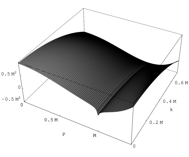
FIG. 4.: Kinetic term $\tilde{\Sigma}_{k}$ in $d=4$ dimensions as a function of ${\rm p}\equiv|p|$ and the cutoff $k$.

The behaviour of the various kinetic terms is illustrated in figures 3 and 4 by means of two different kinds of plots. In the 3D-plot the kinetic term is presented as a function of the two variables $|p|$ and $k$ whereas the 2D-plots show certain slices of the corresponding 3D-plots at distinct $k$-values. (We have displayed only one of the 3D-plots here.) Since for $k\geq M/\sqrt{2}$ the kinetic term is not renormalized and thus does not flow at all, each plot starts at $k=M/\sqrt{2}\equiv k_{\rm cr}$.

Obviously the plots reflect the same qualitative behaviour for the values of $d$ considered here. At $k=k_{\rm cr}$ the kinetic term is given by $\Omega(p^{2})$ which is characterized by the features discussed above. As we move on towards smaller scales $k$ the whole function is lifted so that the $p$-region where the kinetic term $\tilde{\Sigma}_{k}(|p|)$ takes negative values shrinks more and more. Finally, at $k=0$, $\tilde{\Sigma}_{k}(|p|)$ has become completely nonnegative rendering the theory stable. In the course of this evolution the kinetic term builds up a downward peak at $|p|=M$ which grows sharper while the theory is evolved towards smaller values of $k$. At the point $|p|=M$, $\tilde{\Sigma}_{k=0}(|p|)$ has a cusp-type singularity at which it is nondifferentiable but still continuous. It is the shape of this cusp that makes up the main difference between the results for $d=2$ (which we have determined but not displayed here), $d=3$ and $d=4$. Obviously it turns sharper as we increase the dimensionality. The dressed inverse propagator $\Omega_{\rm eff}\equiv\Sigma_{k=0}$ had been presented in the introduction already (FIG. 1).

VIII Regions in field space without classical renormalization

The results for the effective average action derived so far concentrated on the structure of its kinetic term for small $\phi$. In the following sections we discuss the essential features of the complete effective average action and of the potential for our model.

In section IV it was pointed out that there are regions in $\phi$-space where no classical renormalization occurs and thus

$$\Gamma_{k}\left[\phi\right]=S[\phi]=\int d^{d}x\left\{\phi^{*}\,\Omega(-\Box)\,\phi+\frac{\lambda}{2}\left|\phi\right|^{4}\right\}\,.$$ (113)

Obviously we obtain $\Gamma_{k}=S$ for the whole $\phi$-space if $k\geq k_{\rm cr}$, since then $\hat{S}_{k}^{(2)}[\chi]$ is positive definite for any $\chi$.

Let us now consider the case $k<k_{\rm cr}$. It follows immediately from the discussion in section IV that no classical renormalization is expected for those $\phi$ which differ only slightly from $\chi_{\rm min}$. Furthermore, it is easy to see that as long as $|\phi|$ is sufficiently large we have $\chi_{\rm min}=\phi$ in leading order and thus $\Gamma_{k}=S$. To show this we assume that

$$J=\lambda\,\left|\chi_{\rm min}\right|^{2}\,\chi_{\rm min}$$ (114)

provides a good approximation to the e.o.m. (49) which means that $\chi_{\rm min}$, and thus $J$, are large enough to render the $\omega_{k}(-\Box)$-term negligible. For sources leading to (114) the generating functional $W_{k}$ is then approximately given by

$$W_{k}[J]=-S_{k}^{J}\left[\chi_{\rm min};J\right]=-\int d^{d}x\left\{\frac{\lambda}{2}\,\left|\chi_{\rm min}\right|^{4}-J\,\chi_{\rm min}^{*}-J^{*}\,\chi_{\rm min}\right\}$$ (115)

which coincides with the Legendre-transform of

$$\widetilde{\Gamma}_{k}[\phi]=\int d^{d}x\,\frac{\lambda}{2}\left|\phi\right|^{4}=S[\phi]$$ (116)

where $\phi=\chi_{\rm min}$. If $\int d^{d}x\,\phi^{*}\omega_{k}(-\Box)\phi$ is at least of the same order of magnitude as $\int d^{d}x\,k^{2}|\phi|^{2}$ this implies $\Gamma_{k}=S$. Otherwise we have to assume in addition that $k^{2}|\phi|^{2}<<\lambda|\phi|^{4}$ in order to obtain the same result $\Gamma_{k}=S$. Obviously, in both cases it is the large field $\phi=\chi_{\rm min}$ which causes the Hessian $\hat{S}_{k}^{(2)}[\chi_{\rm min}]$ to be positive definite, thereby acting as a cutoff.

In order to make this argument more precise we restrict our considerations from now on to the subspace of plane-wave fields

$$\phi(x)=A\,\exp(ip_{\mu}x_{\mu}+i\beta)$$ (117)

where $A$ is a real, positive amplitude. We start from the assumption that indeed

$$\Gamma_{k}\left[A\,\exp(ip_{\mu}x_{\mu}+i\beta)\right]=S\left[A\,\exp(ip_{\mu}x_{\mu}+i\beta)\right]\,.$$ (118)

Then the results obtained in appendix A 1 may be applied to (118) in order to determine conditions on the parameter $A$ which tell us when $\Gamma_{k}=S$ is satisfied.

Inserting (117) into (113) and adding the cutoff term $k^{2}\int d^{d}x\,|\phi|^{2}$ leads to

$$\widetilde{\Gamma}_{k}\left[A\,\exp(ip_{\mu}x_{\mu}+i\beta)\right]\equiv{\cal V}\left[U_{k}(A;p^{2})+k^{2}\,A^{2}\right]={\cal V}\left[\omega_{k}(p^{2})\,A^{2}+\frac{\lambda}{2}\,A^{4}\right]$$ (119)

from which we obtain

$$J=\frac{\delta\widetilde{\Gamma}_{k}}{\delta\phi^{*}}\left[A\,\exp\left(ip_{\mu}x_{\mu}+i\beta\right)\right]=\left[\omega_{k}(p^{2})\,A+\lambda\,A^{3}\right]\,\exp\left(ip_{\mu}x_{\mu}+i\beta\right)$$ (120)

By setting $J=\varepsilon\,\exp(ip_{\mu}x_{\mu}+i\beta)$ this equation takes the form

$$\omega_{k}(p^{2})\,A+\lambda\,A^{3}=\varepsilon$$ (121)

which is equivalent to eq. (A5) with $\hat{\chi}_{0}$ replaced with $A$. Thus we can read off the solution of (121) from appendix A 1 which is given by

$$A(\varepsilon;p)=\left\{\begin{array}[]{ll}\chi_{0}(\varepsilon;p)\,,&\omega_{k}(p^{2})\geq 0\\ \tilde{\chi}_{0}(\varepsilon;p)\,,&\omega_{k}(p^{2})<0\end{array}\right.$$ (124)

where $\chi_{0}(\varepsilon;p)$ and $\tilde{\chi}_{0}(\varepsilon;p)$ are defined by eqs. (A6), (A13), respectively. Eqs. (121), (124) may now be used to perform the Legendre-transformation from $\widetilde{\Gamma}_{k}$ to $W_{k}$ which yields

$$W_{k}\left[J=\varepsilon\,\exp(ip_{\mu}x_{\mu}+i\beta)\right] = -{\cal V}\left[\omega_{k}(p^{2})\,A^{2}(\varepsilon;p)+\frac{\lambda}{2}\,A^{4}(\varepsilon;p)-2\varepsilon\,A(\varepsilon;p)\right]$$ (125)

$$= -S_{k}^{J}\left[A(\varepsilon;p)\,\exp(ip_{\mu}x_{\mu}+i\beta);\varepsilon\,\exp(ip_{\mu}x_{\mu}+i\beta)\right]\,.$$ (126)

According to appendices A 1, A 2 this expression equals $-S_{k}^{J}[\chi_{\rm min};J]$ if and only if either (I): $k\geq k_{\rm cr}$ or (II): $k<k_{\rm cr}$ and $A(\varepsilon;p)\geq A_{\rm triv}$. Here

$$A_{\rm triv}\equiv\hat{\chi}_{0}=\sqrt{\frac{1}{2\lambda}(M^{2}-2k^{2})}$$ (127)

denotes the critical value of the amplitude beyond which $\Gamma_{k}$ becomes trivial, i.e. equal to $S$. It depends on $k$ but is independent of the momentum $p$. At the initial point $k=k_{\rm cr}$ we have $A_{\rm triv}=0$, but when we lower $k$ $A_{\rm triv}$ grows and the $A$-interval with nontrivial renormalization effects expands.

In terms of the effective potentials $U_{k}(A;p^{2})$ for plane-wave fields which we defined in eq. (41) the statement $\Gamma_{k}=S$ means that $U_{k}(A;p^{2})$ equals the classical potential

$$U^{(\rm cl)}(A;p^{2})\equiv\Omega(p^{2})\,A^{2}+\frac{\lambda}{2}\,A^{4}\,.$$ (128)

Its minimum is located at

$$A_{\rm min}^{(\rm cl)}(p)=\sqrt{-\frac{1}{\lambda}\Omega(p^{2})}$$ (129)

where it assumes the value

$$U^{(\rm cl)}(A_{\rm min}^{(\rm cl)}(p);p^{2})=-\frac{\Omega^{2}(p^{2})}{2\lambda}$$ (130)

For $k$ not too far below $k_{\rm cr}$, the classical minimum lies in the region with no renormalization ($A_{\rm triv}<A_{\rm min}^{(\rm cl)}$). But, at $k=0$, $A_{\rm triv}$ is always larger than $A_{\rm min}^{(\rm cl)}$, except for $p^{2}=M^{2}$ where $A_{\rm triv}=A_{\rm min}^{(\rm cl)}$.

IX Structure of the effective average action

In the previous section it was shown that the effective average action for plane-wave fields equals $S$ as long as $A\geq A_{\rm triv}(k)$, which will be refered to as the “outer region” of the effective potential. The inner region for $A<A_{\rm triv}(k)$ is characterized by nontrivial instability induced classical renormalization. For $k\geq k_{\rm cr}$ no inner region occurs. For $k<k_{\rm cr}$ the determination of $U_{k}(A;p^{2})$ in the inner region is more involved. Depending on the momentum $p$ several cases are to be distinguished.

A $|p|\neq M$

First of all let us consider the case $|p|\neq M$. The definition of the effective potential

$$\Gamma_{k}\left[A\,\exp(ip_{\mu}x_{\mu}+i\beta)\right]\equiv{\cal V}\,U_{k}(A;p^{2})$$ (131)

corresponds to sources which are plane waves of the form $J=\varepsilon\,\exp\left(ip_{\mu}x_{\mu}+i\beta\right)$. Here $\varepsilon$ is related to $A$, $p$ and $k$ via the source-field relation

$$\varepsilon=\frac{1}{2}\frac{\partial U_{k}(A;p^{2})}{\partial A}+k^{2}\,A\,.$$ (132)

Since according to section VIII and appendix A 1 the outer region $A\geq A_{\rm triv}$ is already parametrized by the $\varepsilon$-values lying in the interval $[\varepsilon_{k}(p^{2}),\infty)$ the inner region of $U_{k}$ must correspond to $\varepsilon$-values in $[0,\varepsilon_{k}(p^{2}))$. The problem is that, in case of $\varepsilon<\varepsilon_{k}(p^{2})$, we do not have an exact expression for the field configurations $\chi_{\rm min}$ which minimize the action $S_{k}^{J}$ globally. Thus we are not able to determine the inner region of the potential $U_{k}(A;p^{2})$ exactly. However, it is still possible to deduce the qualitative structure of $U_{k}(A;p^{2})$ for $A<A_{\rm triv}$ by patching up the available pieces of information.

As in section VII we assume that, at least for sufficiently small $|\phi|$, $\Gamma_{k}$ is analytic in $\phi$ and $\phi^{*}$. Then it follows from U(1)-invariance that $U_{k}(A;p^{2})$ is an even function of $A$ and may be expanded about $A=0$ according to

$$U_{k}(A;p^{2})=-\frac{1}{8\lambda}\left(M^{2}-2k^{2}\right)^{2}+\sum\limits_{n=1}^{\infty}u^{(2n)}_{k}(p)\,A^{2n}\,.$$ (133)

In section VII we already calculated the first coefficient of this expansion $u^{(2)}_{k}(p)=\Sigma_{k}(p^{2})$. In addition, an expression for $u^{(4)}_{k}$ is derived in appendix D. It is given by

$$u^{(4)}_{k}(p)=-\left(\Sigma_{k}(p^{2})+k^{2}\right)^{4}\,G^{(4)}_{k}(p^{2})\,.$$ (134)

The 4-point function $G^{(4)}_{k}(p^{2})$ has an extremely complicated structure; it has been evaluated numerically for some special values of $p$ and $k$ only. Thus we know the behaviour of $U_{k}(A;p^{2})$ for small values of $A$.

On the other hand, we know that $U_{k}(A;p^{2})=\Omega(p^{2})\,A^{2}+(\lambda/2)\,A^{4}$ for $A\geq A_{\rm triv}$.

For the intermediate range of $A$-values where (133) is not applicable any more but $A$ is still below $A_{\rm triv}$ we have to find an interpolation which connects the small-$A$ region to the outer region $A\geq A_{\rm triv}$ in a qualitatively correct manner. We make the most natural assumption that this interpolation is a minimal one in the sense that it leads to as few as possible extrema of $U_{k}$. For instance, if $U_{k}(0;p^{2})<U^{(\rm cl)}(A_{\rm triv};p^{2})$ and if the slope at $A=0$, i.e. $\Sigma_{k}$, is positive we interpolate with a monotonically increasing function from the small-$A$ region up to $A_{\rm triv}$. Likewise, if the slope at $A=0$ is negative the interpolating function is assumed to have a single minimum in the intermediate region.

The justification for this scheme comes from three sources:

• The inclusion of the $A^{4}$-term confirms this picture in a part of the parameter space.

• In the limit $k\rightarrow 0$ it leads to the expected convexity of $U_{0}(A;p^{2})$.

• The resulting $U_{k}(A;p^{2})$ connects smoothly to $U_{k}(A;M^{2})$ which can be evaluated exactly.

We shall discuss momenta $p$ with $\Omega(p^{2})\geq 0$ and $\Omega(p^{2})<0$ separately.

1 The case $\Omega(p^{2})\geq 0$

The case $\Omega(p^{2})\geq 0$ corresponds to $p^{2}$-values lying in $\{0\}\cup[2M^{2},\infty)$. In particular it includes the standard effective potential for $p=0$. Since in this case $\Sigma_{k}>0$ for all $k<k_{\rm cr}$ the minimal interpolation leads to the monotonically increasing function shown in FIG. 5. The shape of this curve changes only insignificantly in the course of the evolution. The only change is a decrease of $C_{k}$ compensated by an increase of the slope of the curve for $A<A_{\rm triv}$ such that (a) the inner and the outer region join smoothly at $A=A_{\rm triv}$ and (b) $U_{k_{2}}(A;p^{2})<U_{k_{1}}(A;p^{2})$ is valid for all $A<A_{\rm triv}$, if $k_{2}<k_{1}\leq k_{\rm cr}$.

FIG. 5.: Qualitative scaling behaviour of $U_{k}(A;p^{2})$ for $p^{2}\in\{0\}\cup[2M^{2},\infty)$, illustrated by three curves corresponding to the $k$-values $k=k_{\rm cr}$ (upper curve), $k=k_{l}$ where $0<k_{l}<k_{\rm cr}$ (curve in the middle) and $k=0$.

The inclusion of the $A^{4}$-term gives additional support to this picture. It turns out that the $A^{2}$-term dominates the behaviour of $U_{k}$ for all $A\leq A_{\rm triv}$ if the difference between $|p|$ and $M$ is large enough. Then higher order terms like $u_{k}^{(4)}$ yield only minor corrections.

(a)

(b)

FIG. 6.: $U^{(\rm cl)}$, $U_{k=0}^{(2)}$ and $U_{k=0}^{(4)}$ (in units of $M^{4}/\lambda$) as functions of $A$ (in units of $M/\sqrt{\lambda}$). (a): Case $p=0$. The curves for $U_{k=0}^{(2)}$ and $U_{k=0}^{(4)}$ are those which coincide at $A=0$, where $U_{k=0}^{(4)}$ corresponds to the curve that develops a negative slope for large $A$. The remaining curve corresponds to $U^{(\rm cl)}$. (b): Case $|p|=3M$. The difference between the three curves is hardly visible. Near $A_{\rm triv}=M/\sqrt{2\lambda}$ we have $U_{k=0}^{(4)}<U^{(\rm cl)}<U_{k=0}^{(2)}$.

In FIG. 6 we plotted $U^{(\rm cl)}(A;p^{2})$ (which coincides with the true $U_{k}$ for $k\geq k_{\rm cr}$, $A$ arbitrary and for $k<k_{\rm cr}$, $A\geq A_{\rm triv}$) and the approximations

$$U_{k}^{(2)}(A;p^{2}) \equiv C_{k}+\Sigma_{k}(p^{2})\,A^{2}$$ (135)

$$U_{k}^{(4)}(A;p^{2}) \equiv C_{k}+\Sigma_{k}(p^{2})\,A^{2}-\left(\Sigma_{k}(p^{2})+k^{2}\right)^{4}G_{k}^{(4)}(p^{2})\,A^{4}$$ (136)

for $p=0$, $k=0$ and for $|p|=3M$, $k=0$. Obviously $p=0$ is not sufficiently far away from $M$ because $U_{0}^{(2)}$ is a good approximation only for very small $A$-values and then grows too fast to be able to merge with $U^{(\rm cl)}$ at $A_{\rm triv}$. The effect of the $A^{4}$-term is to bend this curve downward. Hence $U_{0}^{(4)}$ is already fairly accurate for a larger range of $A$-values and it gets closer to the $U^{(\rm cl)}$-curve. For $A$ approaching $A_{\rm triv}$ also the $A^{4}$-approximation breaks down and it is clear that higher orders are needed in order to hit the $U^{(\rm cl)}$-curve at $A_{\rm triv}$.

For $|p|=3M$ the situation is much better. $U^{(\rm cl)}$, $U_{0}^{(2)}$ and $U_{0}^{(4)}$ are virtually identical for all $A\leq A_{\rm triv}=M/\sqrt{2\lambda}$. (This is because $\Sigma_{k=0}(p^{2})\approx\Omega(p^{2})$ for large $p$.) Due to the corrections coming from the $A^{4}$-term we expect that $U_{0}^{(4)}$ agrees better with the exact $U_{0}$ than $U_{0}^{(2)}$ but the difference between the two approximations is too tiny to be visible. However, we surely can infer from FIG. 6 that both $U_{0}^{(2)}$ and $U_{0}^{(4)}$ are convex. For even larger momenta the quality of the approximation (133) increases.

From the general properties of Legendre transforms we expect $\lim_{k\rightarrow 0}U_{k}(A;p^{2})$ to be a convex function of $A$, for all values of $p$. For the momenta considered here this convexity is indeed achieved, albeit in a somewhat trivial fashion since the potential was convex from the outset.

2 The case $\Omega(p^{2})<0$

Let us now turn to the case $\Omega(p^{2})<0$, $|p|\neq M$, which is satisfied by all values of $p^{2}$ contained in $(0,2M^{2})\setminus\{M^{2}\}$. For such momenta the $A^{2}$-expansion (133) yields no reliable results because the higher order terms begin to dominate already at small values of $A<A_{\rm triv}$. Those results are at most as reliable as the one for $p=0$, $k=0$ and they become increasingly worse as $|p|$ approaches $M$. Hence we have to apply a different method to determine the properties of $U_{k}$ in the inner region.

First of all it should be noted that in the course of the evolution $\Sigma_{k}(p^{2})$ changes its sign which is obvious from the FIGS. 3 and 4. There exists a scale $\hat{k}(p)<k_{\rm cr}$ at which $\Sigma_{\hat{k}}(p^{2})=0$; we have $\Sigma_{k}<0$ for $k>\hat{k}$ and $\Sigma_{k}>0$ for $k<\hat{k}$.

Along with the evolution of $\Sigma_{k}$, i.e. the slope of $U_{k}$ at $A=0$, the constant term $U_{k}(A=0;p^{2})=C_{k}$ drops from $C_{k}=0$ at $k=k_{\rm cr}$ to $C_{k}=-M^{4}/(8\lambda)$ at $k=0$. If one minimally interpolates between this small-$A$ behaviour and $U^{(\rm cl)}$ one obtains the curves shown in FIG. 7. Note that the change of sign of $\Sigma_{k}$ is crucial for achieving convexity in the limit $k\rightarrow 0$. As long as $k>\hat{k}(p)$, $U_{k}$ is not convex since the negative kinetic term $\Sigma_{k}$ causes $U_{k}$ to decrease for very small values of $A$.

FIG. 7.: Qualitative scaling behaviour of $U_{k}(A;p^{2})$ for $p^{2}\in(0,2M^{2})\setminus\{M^{2}\}$, illustrated by three curves corresponding to the $k$-values $k=k_{\rm cr}$ (upper curve), $k=k_{0}$ where $0<k_{0}<k_{\rm cr}$ (curve in the middle) and $k=0$.

In FIG. 7 we included an additional piece of information which is easy to obtain. There exists a certain scale $k_{0}(p)\in(0,k_{\rm cr})$ at which the value of the potential at $A=0$ equals its value at $A_{\rm triv}$: $U_{k_{0}(p)}(0;p^{2})=U_{k_{0}(p)}(A_{\rm triv};p^{2})$. This means that $C_{k_{0}(p)}=U^{(\rm cl)}(A_{\rm triv};p)$, and by eq. (98) this condition is equivalent to $\Omega(p^{2})=k_{0}^{2}-M^{2}/2$. Hence

$$k_{0}(p)=\frac{1}{\sqrt{2}M}\left|M^{2}-p^{2}\right|\,.$$ (137)

Numerically we find that $k_{0}(p)<\hat{k}(p)$ for any value of $p$ considered here. Therefore the slope at the origin is positive for $k=k_{0}$. Since, at $A_{\rm triv}$, $U^{(\rm cl)}$ has a positive slope too this means that $U_{k}$ has (at least) one maximum and one minimum in the inner region. (The minimum is the expected one, of course, essentially the minimum of $U^{(\rm cl)}$, corrected by the renormalization effects.) In order to obtain a convex potential in the limit $k\rightarrow 0$ this local maximum must shrink as the theory is evolved towards smaller $k$ until it vanishes at some scale between $k_{0}(p)$ and zero.

The results derived so far are sufficient to give a qualitative discription of $U_{k}$ in the inner region. FIG. 7 illustrates its essential features as well as the exact structure of the effective potential in the outer region. Again, the effective average potential becomes convex in the limit $k\rightarrow 0$, this time in a less trivial fashion though.

B $|p|=M$

Let us finally come to the “resonant” case $|p|=M$. It will turn out that an exact expression for $U_{k}$ can be derived in this case.

As in the case before we obtain from U(1)-invariance

$$\Gamma_{k}\left[A\,\exp\left(iQ_{0\mu}x_{\mu}+i\beta\right)\right]\equiv{\cal V}\,U_{k}(A;M^{2})$$ (138)

where the corresponding sources are plane waves satisfying the source-field relation (132) with $p$ replaced with $Q_{0}$. From section VIII and appendix A 1 we know that any source-amplitude $\varepsilon>0$ is related to a field-amplitude $A\in(A_{\rm triv},\infty)$ via eq. (132) and that $\varepsilon=0$ yields $A_{\rm triv}$. Actually $\varepsilon=0$ corresponds to the complete inner region $A<A_{\rm triv}$ as well. To see this we have to look at the generating functional $W_{k}$ evaluated at $J=\varrho\,\exp(iQ_{0\mu}x_{\mu})$ where $\varrho\equiv\varepsilon\,\exp(i\beta)$ is complex. Inserting the global minimum $\chi_{\rm min}$ in presence of plane-wave sources, eq. (A10), into $W_{k}[J]=-S_{k}^{J}[\chi_{\min}(J);J]$ and expanding this expression with respect to $|\varrho|\equiv\varepsilon$ about $|\varrho|=0$ yields

$$W_{k}\left[J=\varrho\,\exp(iQ_{0\mu}x_{\mu})\right]$$ (139)

$$= {\cal V}\,\left[\frac{\omega_{k}^{2}(M^{2})}{2\lambda}+2\,|\varrho|\,\sqrt{-\frac{1}{\lambda}\omega_{k}(M^{2})}-\frac{|\varrho|^{2}}{2\,\omega_{k}(M^{2})}\right]+{\cal O}(|\varrho|^{3})\,.$$ (140)

The crucial point is that the term linear in $|\varrho|$ causes $dW_{k}/d\varrho$ to be discontinuous at $\varrho=0$. In fact we obtain from (139)

$$\lim\limits_{|\varrho|\rightarrow 0}\left[\frac{d}{d\varrho}W_{k}\left[\varrho\,\exp(iQ_{0\mu}x_{\mu})\right]\right]_{\varrho=|\varrho|\exp(i\beta)}=\sqrt{-\frac{1}{\lambda}\omega_{k}(M^{2})}\,\exp(-i\beta)\equiv A_{\rm triv}\,\exp(-i\beta)$$ (141)

which shows that this derivative depends on $\beta$, i.e. on the direction in the complex plane from which $\rho=0$ is approached.

This singular behaviour has the effect that the conventional Legendre-transformation is not applicable. In such cases one has to refer to the more general supremum-definition of the Legendre-transformation, see e.g. [10]. In our case it amounts to

$$U_{k}(A;M^{2})=-k^{2}\,A^{2}+\sup\limits_{\varepsilon\geq 0}\left\{2A\,\varepsilon-F_{k}(\varepsilon;Q_{0})\right\}$$ (142)

where

$$F_{k}(\varepsilon;Q_{0}) \equiv \frac{1}{{\cal V}}W_{k}\left[\varepsilon\,\exp(iQ_{0\mu}x_{\mu}+i\beta)\right]$$ (143)

$$= 2\varepsilon\,\tilde{\chi}_{0}(\varepsilon;Q_{0})-\omega_{k}(M^{2})\,\tilde{\chi}_{0}^{2}(\varepsilon;Q_{0})-\frac{\lambda}{2}\,\tilde{\chi}_{0}^{4}(\varepsilon;Q_{0})$$ (144)

with $\tilde{\chi}_{0}$ defined in (A13). Using eq. (A5) $F_{k}$ may be rewritten as

$$F_{k}(\varepsilon;Q_{0})=\frac{3}{2}\varepsilon\,\tilde{\chi}_{0}(\varepsilon;Q_{0})-\frac{1}{2}\omega_{k}(M^{2})\,\tilde{\chi}_{0}^{2}(\varepsilon;Q_{0})\,.$$ (145)

Since $\tilde{\chi}_{0}(\varepsilon;Q_{0})$ is a strictly monotonically increasing function of $\varepsilon$ we can infer from eq. (145) that $F_{k}$ is strictly convex. (This is of course as it should be because in our classical approximation $W_{k}$ is related to $S_{k}$ via a Legendre-transformation.) Therefore the strict inequality

$$\frac{\partial F_{k}}{\partial\varepsilon}(\varepsilon)>\frac{\partial F_{k}}{\partial\varepsilon}(\varepsilon=0)\equiv 2\sqrt{-\frac{1}{\lambda}\omega_{k}(M^{2})}\equiv 2\,A_{\rm triv}$$ (146)

is satisfied for all $\varepsilon>0$. It implies that as long as we have $A<A_{\rm triv}$ the supremum of $2A\,\varepsilon-F_{k}(\varepsilon;Q_{0})$ is always achieved for $\varepsilon=0$ where it has the value $C_{k}$. As a consequence the complete inner region $[0,A_{\rm triv}]$ corresponds to $\varepsilon=0$ and the length of this interval is determined by the linear term of $F_{k}$. For $A>A_{\rm triv}$ the supremum-definition coincides with the familiar definition of the Legendre-transformation so that eq. (142) leads to

$$U_{k}(A;M^{2})=\left\{\begin{array}[]{ll}C_{k}-k^{2}\,A^{2}&{\rm if}\;A\leq A_{\rm triv}\\ U^{(\rm cl)}(A;M^{2})&{\rm if}\;A>A_{\rm triv}\end{array}\right.\,.$$ (149)

The behaviour of $U_{k}$ is illustrated in FIG. 8 which contains several curves obtained from eq. (149) for distinct values of $k$. The case $|p|=M$ is special in that $C_{k=0}$ equals exactly the value of $U^{(\rm cl)}$ at its minimum $A_{\rm min}^{(\rm cl)}$, and also because it is precisely $A_{\rm min}^{(\rm cl)}$ which separates the inner from the outer region, i.e. $A_{\rm triv}=A_{\rm min}^{(\rm cl)}$. As a consequence the inner region of $U_{k}$ approaches a constant value as the cutoff is lowered from $k=k_{\rm cr}$ towards $k=0$. At $k=0$ the inner region is entirely flat and thus $U_{k=0}$ is found to be convex.

FIG. 8.: Scaling behaviour of $U_{k}(A;M^{2})$, illustrated by six curves corresponding to different values of $k$. With decreasing $k$ the inner region appoaches a constant value.

Note that, as it should be, the functional $\widetilde{\Gamma}_{k}$ is always convex even in situations where $U_{k}$, i.e. $\Gamma_{k}$ is not. Comparing (41) to (119) we see that $\widetilde{\Gamma}_{k}$ yields $\widetilde{U}_{k}\equiv U_{k}+k^{2}A^{2}$ when evaluated for plane waves. For instance, from eq. (149) it follows that $\widetilde{U}_{k}=C_{k}$ if $A\leq A_{\rm triv}$ and $\widetilde{U}_{k}=U^{(\rm cl)}+k^{2}A^{2}$ if $A>A_{\rm triv}$, which is perfectly convex for any value of $k$.

The physical interpretation of this behaviour of $W_{k}$ and $\Gamma_{k}$ is as follows. Eq. (141) is nothing but the standard formula

$$\left.\frac{\delta W_{k}}{\delta J^{*}}\right|_{J=0}=\left.\left<\chi\right>\right|_{J=0}\equiv\left<\chi\right>$$ (150)

evaluated for plane waves. Let us look at this equation for $k=0$. The nonvanishing r.h.s. of eq. (141) shows that the modes with $|p|=M$ acquire a vacuum expectation value. After the source $J$ has been switched off adiabatically the expectation value

$$\left<\chi(x)\right>=\frac{M}{\sqrt{2\lambda}}\,\exp\left(iMn_{\mu}x_{\mu}+i\beta\right)$$ (151)

“remembers” both the direction $n_{\mu}$ and the phase $\beta$ of the source. This singles out a point $(n,\beta)$ of the vacuum manifold and leads to a spontaneous breaking of both the ISO($d$) symmetry of spacetime rotations and of the U(1) phase symmetry.

This formation of a vacuum condensate happens only for the modes with $|p|=M$ but not for $|p|\neq M$. The difference of the two cases is nicely illustrated by the plots of the various effective potentials. Let us look at FIG. 7 for $|p|\neq M$, say, and let us put a “ball” into the minimum of the potential $U_{k}$ at $k=k_{\rm cr}$. Then, when we lower $k$, at a certain point the ball rolls down from the local minimum at $A\neq 0$ to the minimum at $A=0$. Thus, for $k=0$, the corresponding field mode has no expectation value. The situation is different in FIG. 8 for $|p|=M$. Until the very last moment of the evolution the ball always sits at the global minimum of the potential and has no tendency to roll towards $A=0$. Only for a strictly vanishing cutoff $k$, $U_{k}(A=0;M^{2})$ is as low as $U_{k}$ at the minimum. This means that the corresponding mode acquires an expectation value. In fact, our discussion here is remarkably similar to the analogous treatment of the familiar spontaneous symmetry breaking by a Mexican-hat potential. In the latter case it is the $(p=0)$-modes which condense, but in the language of the generalized effective average potentials $U_{k}$ for arbitrary momenta this makes no conceptual difference.

Within the present approximation the true vacuum consists of a single plane wave. Therefore this field configuration serves as a “master field” from which the expectation value of any composite operator can be computed by simply inserting the r.h.s. of eq. (151). For $\partial_{\mu}\chi^{*}\,\partial_{\mu}\chi$, say, this leads to the kinetic condensate (11) announced in the introduction.

X Conclusion

In this paper we investigated a scalar model with a nonstandard inverse propagator consisting of a destabilizing $-p^{2}$-term and a stabilizing $+p^{4}$-term. We find that this model exhibits both spontaneous breaking of translation symmetry and of a global U(1) phase symmetry. The ground state respects, nevertheless, a modified combined translation symmetry which also involves phase rotations. The rotation symmetry is broken from SO($d$) to SO($d-1$). In classical or quantum statistical systems our model describes the spontaneous formation of layers in an otherwise homogeneous and isotropic setting. For such models already a tiny perturbation leads to the formation of a geometrical structure.

In order to gain a detailed understanding how the instabilities are removed from the effective action by including the effects of fluctuations we have performed a renormalization group analysis. In particular, we have calculated the renormalization group flow of the dressed inverse propagator $\Sigma_{k}(p^{2})$ for zero fields and of the finite-momentum effective potentials $U_{k}(A;p^{2})$ in leading order of the semiclassical expansion. We found strong renormalization effects which are “instability induced” rather than “fluctuation induced”. They are driven by the classical instability of the trivial saddle point in certain regions in the space of field configurations. This is related to the fact that the global minimum of the Euclidean action $S[\chi]$ is not at $\chi=0$. Instead, it is realized by nontrivial spin-wave configurations which form a space $S^{1}\times S^{d-1}$ of classical vacua. At the level of the effective theory, we found that the theory stabilizes itself in a dynamical way. The dressed kinetic operator $\Omega_{\rm eff}\equiv\Sigma_{k=0}$ gives a strictly positive action to all field modes with momenta $|p|\neq M$. For modes with $|p|=M$ it vanishes. These modes are stabilized by a “shift to the true vacuum” which is similar to what happens in standard spontaneous symmetry breaking with a Mexican-hat potential. The modes with $|p|=M$ form a spatially nonuniform, Poincaré- and phase-symmetry breaking condensate. Within the semiclassical approximation, the true vacuum consists of a single spin wave of momentum $M$ and amplitude $M/(2\lambda)$, and is of an obviously nonperturbative nature therefore. The fixed phase and direction of this spin wave lead to a spontaneous breaking of the classical U(1)$\times$ISO($d$) symmetry.

In this paper we only have considered a model without a classical mass term. Due to our particular choice of the infrared cutoff ${\cal R}_{k}=k^{2}$ generalized results for models with a mass term can easily be infered from our results for nonvanishing $k$.

In the introduction we mentioned that a strong motivation for studying this model is its similarity with Euclidean quantum gravity based upon actions such as $\int d^{d}x\,\sqrt{g}\left\{\alpha\,R+\beta\,R^{2}\right\}$. For the conformal factor of the metric such an action contains a negative contribution to the kinetic energy, coming from $\sqrt{g}R$ and dominating at momenta small compared to the Planck mass. At large momenta the action becomes positive and all modes are stable because of the manifestly positive contribution arising from $\sqrt{g}R^{2}$. In view of this analogy it is plausible to speculate that also quantum gravity dynamically stabilizes the conformal factor by developing a nontrivial vacuum structure, with nonzero condensates such as $\left<(\bar{D}_{\mu}\phi)^{2}\right>$, so that all excitations about this ground state are stable.

In the scalar model the semiclassical expansion about $\chi_{\rm min}$, the global minimum of $S_{k}^{J}$, has led to an effective kinetic operator $\Omega_{\rm eff}(p^{2})$ which has stabilized (almost) all modes which were unstable with respect to the classical $\Omega(p^{2})$. In gravity we might expect a similar mechanism to be at work when we expand about the global minimum of $\int d^{d}x\,\sqrt{g}\left\{\alpha\,R+\beta\,R^{2}\right\}$. Roughly speaking, leaving finer details of the momentum dependence aside, the $\Omega_{\rm eff}(p^{2})$-curve is obtained from $\Omega(p^{2})$ by shifting it upward by a constant $(\rm mass)^{2}$-term $M^{2}/2$, see FIG. 1. So the dynamical stabilization of the scalar model is essentially a “mass generation”.

This mass generation also provides the justification for our loop expansion and retaining the lowest order contribution only. Contrary to the case of massless models with an ordinary kinetic term where the loop expansion does not lead to reliable results [11], in our model the mass generation cuts off loops so that the loop correction to $\lambda$, for instance, is negligible.

It is an important question how a similar mass generation would manifest itself in the effective average action for gravity, $\Gamma_{k}[g_{\mu\nu}]$, and which type of truncations should be used in order to obtain it from the flow equation [12]. It is clear that a naive mass term for the conformal factor is forbidden by general coordinate invariance. But also local curvature invariants $R^{2}$, $R_{\mu\nu}R^{\mu\nu}$ etc. are of no help because they vanish for flat space and will not lead to an effective action whose minimum is at $g_{\mu\nu}=\delta_{\mu\nu}$ [13]. This suggests that the relevant terms in $\Gamma$ and $\Gamma_{k}$ must be nonlocal if expressed in a gauge invariant way. (After gauge fixing, they may be local, nevertheless.) For instance, a higher dimensional analogue of the $2d$ induced gravity action $\int d^{d}x\,\sqrt{g}\,R\,\Box^{-1}\,R$, added to the Einstein-Hilbert term, is known to have flat space as its global minimum [13]. Hence all fluctuations about this ground state, including those of the conformal factor, are stable. Therefore it would be very interesting to study the renormalization group flow of $\Gamma_{k}[g_{\mu\nu}]$ using a truncation of the space of actions which includes nonlocal invariants. Work along these lines is in progress.

One may wonder if the analogy between our model and gravity can be put even further. In a gauge fixed version of gravity the local symmetry of general coordinate transformations may be “spontaneously broken”, similar to the Higgs-picture for local gauge theories. This language is usually employed in order to describe spontaneous compactification of higher dimensional theories. The fact that the minimum of the Euclidean action occurs for a non-translationally invariant field configuration then strongly suggests the existence of additional space dimensions, $d>4$. Otherwise, for $d=4$, the spectrum of excitations may not exhibit the full four-dimensional Poincaré symmetry, similar to the spectrum shown in FIG. 2. In higher dimensions, the $d$-dimensional Poincaré symmetry may be reduced to a four-dimensional Poincaré symmetry, again similar to our example. Actually, classical solutions with spontaneous compactification which have a lower Euclidean action than flat $d$-dimensional space have been discussed a long time ago [14]. In view of the present paper it would be very interesting to find realistic classical solutions corresponding to the absolute minimum of the Euclidean action.

A Global minimum for plane-wave sources

In this part of the appendix we concentrate on determining the global minimum of the action $S_{k}^{J}$ for plane-wave sources $J=\varepsilon\,\exp\left(ip_{\mu}x_{\mu}+i\beta\right)$. In the first subsection we discuss two kinds of solutions, each of them yielding the global minimum in a certain range of the $(\varepsilon,p,k)$-parameter space. In the second subsection the function $\varepsilon_{k}(p^{2})$, which describes the region in the parameter space separating these ranges, is exactly derived. The third subsection of this appendix contains additional calculational details needed for obtaining some of the results given in the first subsection.

1 Solutions of the e.o.m.

For the calculation of the effective average action for plane-wave average fields (see section IX) it is necessary to find out some properties of the solutions corresponding to nonvanishing sources which are plane waves of the form

$$J(x)=\varepsilon\,\exp\left(ip_{\mu}x_{\mu}+i\beta\right)$$ (A1)

with a real “amplitude” $\varepsilon\geq 0$ and $\beta\in[0,2\pi)$. This restriction allows us to calculate the minimizing field configurations either exactly (for $k^{2}\geq M^{2}/2$) or at least approximately for small values of $\varepsilon$ (for $k^{2}\leq M^{2}/2$).

For the source (A1), the e.o.m. we have to solve takes the form

$$\left[\Omega(-\Box)+k^{2}+\lambda\,\left|\chi\right|^{2}\right]\chi=\varepsilon\,\exp\left(ip_{\mu}x_{\mu}+i\beta\right).$$ (A2)

a The solution $\chi\propto\exp(ipx+i\beta)$

The simplest solution one can think of is a field $\chi$ which does not “know” about the existence of the nontrivial, degenerate minimum found for $J=0$ and oscillates with the same frequency and phase as the source. If we insert the corresponding ansatz

$$\chi(x)=\chi_{0}\,\exp\left(ip_{\mu}x_{\mu}+i\beta\right)$$ (A3)

into the e.o.m., the result is the $x$-independent equation

$$\omega_{k}(p^{2})\,\chi_{0}+\lambda\,\left|\chi_{0}\right|^{2}\,\chi_{0}=\varepsilon\,.$$ (A4)

As we chose $\varepsilon$ to be real, $\chi_{0}$ must also be real, so that eq. (A4) boils down to a simple cubic equation in the real variable $\chi_{0}$:

$$\chi_{0}^{3}+\frac{\omega_{k}(p^{2})}{\lambda}\,\chi_{0}-\frac{\varepsilon}{\lambda}=0$$ (A5)

The general solution of this equation is given by

$$\chi_{0}(\varepsilon;p)=\left(\frac{\varepsilon}{2\lambda}+\sqrt{\frac{\varepsilon^{2}}{4\lambda^{2}}+\frac{\omega_{k}^{3}(p^{2})}{27\lambda^{3}}}\right)^{1/3}+\left(\frac{\varepsilon}{2\lambda}-\sqrt{\frac{\varepsilon^{2}}{4\lambda^{2}}+\frac{\omega_{k}^{3}(p^{2})}{27\lambda^{3}}}\right)^{1/3}\,.$$ (A6)

We have to distinguish the two cases where

$$\Delta\equiv\frac{\varepsilon^{2}}{4\lambda^{2}}+\frac{\omega_{k}^{3}(p^{2})}{27\lambda^{3}}$$ (A7)

is either positive or negative. If it is positive, the above amplitude $\chi_{0}(\varepsilon;p)$ represents a single real solution of eq. (A5). But if it is negative, the square root of $\Delta$ becomes imaginary, so that $\chi_{0}(\varepsilon;p)$ comprises three different real solutions. Those can be rewritten in the manifestly real form

$$\chi_{0}^{(n)}(\varepsilon;p)=2\sqrt{-\frac{\omega_{k}(p^{2})}{3\lambda}}\,\cos\left[\frac{1}{3}\arccos\left(\frac{\varepsilon}{2}\sqrt{-\frac{27\lambda}{\omega_{k}^{3}(p^{2})}}\right)+\frac{2\pi n}{3}\right]\;,\;\;n=0,1,2.$$ (A8)

However, one can check easily that the only candidate for the global minimum is $\chi_{0}^{(n=0)}$, because the action corresponding to this branch is lower than the action corresponding to the other two branches. Taking into account that the branch $\chi_{0}^{(n=0)}$ is the only one that coincides with eq. (A6) at $\Delta=0$, this result is not very surprising.

Combining the above expressions, which describe potential minima in the two complementary regions of $\Delta$, we can formulate solutions for the whole range of $\Delta$ and thus also of $\varepsilon$. We have to consider two distinct cases. For $\omega_{k}(p^{2})\geq 0$, $\Delta$ is always nonnegative, so the candidate for the global minimum reads

$$\chi_{\rm min}(x)=\left[\left(\frac{\varepsilon}{2\lambda}+\sqrt{\Delta}\right)^{1/3}+\left(\frac{\varepsilon}{2\lambda}-\sqrt{\Delta}\right)^{1/3}\right]\,\exp\left(ip_{\mu}x_{\mu}+i\beta\right).$$ (A9)

For $\omega_{k}(p^{2})<0$, we have to fit together the two relevant solutions for $\Delta\geq 0$ and $\Delta<0$, so that

$$\chi_{\rm min}(x)=\tilde{\chi}_{0}(\varepsilon;p)\,\exp\left(ip_{\mu}x_{\mu}+i\beta\right)$$ (A10)

where

$$\tilde{\chi}_{0}(\varepsilon;p)=\left\{\begin{array}[]{c}\left(\frac{\varepsilon}{2\lambda}+\sqrt{\Delta}\right)^{1/3}+\left(\frac{\varepsilon}{2\lambda}-\sqrt{\Delta}\right)^{1/3}\;,\;\;\Delta\geq 0\\ 2\sqrt{-\frac{\omega_{k}(p^{2})}{3\lambda}}\,\cos\left[\frac{1}{3}\arccos\left(\frac{\varepsilon}{2}\sqrt{-\frac{27\lambda}{\omega_{k}^{3}(p^{2})}}\right)\right]\;,\;\;\Delta<0\end{array}\right.\,.$$ (A13)

b Is $\chi\propto\exp(ipx+i\beta)$ the global minimum?

What remains to be dealt with is the question whether the solutions (A9), (A10) constitute absolute minima or just saddle points. First we check this for large values of $k$, $k^{2}\geq M^{2}/2$:
In this region the relation $\omega_{k}(p^{2})\geq 0$ is always satisfied which means that $\Delta$ cannot become negative. If we take the corresponding solution, eq. (A9), and send $\varepsilon$ to zero, we end up with $\chi_{\rm min}=0$, which was already shown to be the minimizing field configuration for $J=0$. In addition, it is clear that the integral

$$\int\frac{d^{d}q}{(2\pi)^{d}}\,\left|\widetilde{\delta\chi}(q)\right|^{2}\,\left\{\Omega(q^{2})+k^{2}+\lambda\,\left[\left(\frac{\varepsilon}{2\lambda}+\sqrt{\Delta}\right)^{1/3}+\left(\frac{\varepsilon}{2\lambda}-\sqrt{\Delta}\right)^{1/3}\right]^{2}\right\}$$ (A14)

is always nonnegative (remember that $\omega_{k}(q^{2})=\Omega(q^{2})+k^{2}\geq 0$ for $k^{2}\geq M^{2}/2$) and thus $\Delta S_{k}\geq 0$ is satisfied. Consequently we can identify (A9) as the field that corresponds to the absolute minimum for $k^{2}\geq M^{2}/2$; it coincides with the result of section V if we set $\varepsilon=0$.

Next we investigate the case $k^{2}<M^{2}/2$. The amplitudes of the solutions corresponding to both $\omega_{k}(p^{2})\geq 0$ and $\omega_{k}(p^{2})<0$ grow monotonically, as we increase $\varepsilon$, without approaching any finite bound. This means that, for sufficiently large values of $\varepsilon$, $\lambda|\chi_{\rm min}|^{2}$ will always compensate any possible negative value of $\omega_{k}(q^{2})\geq-M^{2}/2$, rendering the integrals (A14) or

$$\int\frac{d^{d}q}{(2\pi)^{d}}\,\left|\widetilde{\delta\chi}(q)\right|^{2}\,\left[\Omega(q^{2})+k^{2}+\lambda\,\tilde{\chi}_{0}^{2}(\varepsilon;p)\right]$$ (A15)

and thus $\Delta S_{k}$ positive. On the other hand the solutions (A9), (A10) do not approach the nontrivial, degenerate solution (64) as we send $\varepsilon$ to zero. (Even for momenta $p_{\mu}=Mn_{\mu}$, $|n|=1$, the limit $\varepsilon\rightarrow 0$ produces only a unique solution of the form (64), with the unit vector $n$ and the phase $\beta$ fixed.) In view of this behaviour we can state that for any momentum $p$ with $|p|\neq M$ there exists a certain value $\varepsilon_{k}(p^{2})>0$, so that for all $\varepsilon\geq\varepsilon_{k}(p^{2})$ one of the solutions (A9) or (A10) yields the absolute minimum; it depends on the value of $\omega_{k}(p^{2})$ whether (A9) or (A10) is the right one. This implies that for $\varepsilon$-values below the corresponding boundary value $\varepsilon_{k}(p^{2})$ any of the above solutions becomes unstable under certain deformations and therefore is a saddle point or a local extremum. For sufficiently small $\varepsilon$-values the true global minimum must be a generalization of the nontrivial minimum we calculated for the case of vanishing sources.

An upper bound for $\varepsilon_{k}$: Due to the condition (53) we can find an upper bound $\tilde{\varepsilon}_{k}(p^{2})$ for the amplitude $\varepsilon_{k}(p^{2})$, where the transition from one $\varepsilon$-region to the other takes place. All we have to do is to insert $\chi_{0}=\hat{\chi}_{0}$ - this is the lowest value for $\chi_{0}$, for which the first integral of eq. (55) is manifestly positive (or zero) - into eq. (A5) and calculate the corresponding amplitude $\varepsilon$. The result is

$$\tilde{\varepsilon}_{k}(p^{2})=\frac{1}{2M^{2}}\,\sqrt{-\omega_{k}(M^{2})/\lambda}\left(p^{2}-M^{2}\right)^{2}.$$ (A16)

We can turn the above condition on $\varepsilon$ into a condition on the momentum of the source $p$. It follows immediately that for all $\varepsilon$ there exists a momentum $p_{k}(\varepsilon)$, so that for all $p^{2}$ satisfying the relation

$$\max(0,M^{2}-p_{k}^{2}(\varepsilon))\leq p^{2}\leq M^{2}+p_{k}^{2}(\varepsilon)$$ (A17)

the solutions (A9) and (A10) represent absolute minima. A lower bound $\tilde{p}_{k}^{2}(\varepsilon)$ for $p_{k}^{2}(\varepsilon)$ is given by the expression

$$\tilde{p}_{k}^{2}(\varepsilon)=\sqrt{\frac{2M^{2}\,\varepsilon}{\sqrt{-\omega_{k}(M^{2})/\lambda}}}\leq p_{k}^{2}(\varepsilon).$$ (A18)

(In appendix A 2 we proof that indeed $\tilde{\varepsilon}_{k}(p^{2})=\varepsilon_{k}(p^{2})$ and thus $\tilde{p}_{k}^{2}(\varepsilon)=p_{k}^{2}(\varepsilon)$.)

The exceptional case $|p|=M$: For momenta $p_{\mu}=Q_{0\mu}=Mn_{\mu}$, $|n|=1$, the situation is more subtle. For all $\varepsilon>0$ we have $\tilde{\chi}_{0}(\varepsilon;Q_{0})>\hat{\chi}_{0}$. Hence, if $\varepsilon>0$, the corresponding solution (A10) represents the absolute minimum. The phase and the direction of the momentum vector of this solution are uniquely determined by the corresponding parameters of the source. This is still the case for $\varepsilon\rightarrow 0$, where the solution takes the form $\hat{\chi}_{0}\,\exp(iMn_{\mu}x_{\mu}+i\beta)$ with $n_{\mu}$, $\beta$ fixed. Despite of the fact that the integral (A15) is nonnegative for this solution, it does not really yield the true vacuum for vanishing sources, which is degenerate with respect to the phase and the direction of the momentum $Q_{0}$. Thus we recognize a discontinous behaviour concerning the degeneracy of the true vacuum when we switch on sources of the form $\varepsilon\,\exp(iQ_{0\mu}x_{\mu}+i\beta)$. This is analogous to the “tilting” of a Mexican-hat potential caused by a symmetry breaking source.

c Perturbative expansion about $\chi_{\rm min}(J=0)$

Let us now return to the case $p_{\mu}\neq Mn_{\mu}$. As mentioned before, the solution for sufficiently small $\varepsilon$ has to depend on $\varepsilon$ in such a way that it approaches the degenerate solution (64) for $\varepsilon\rightarrow 0$. As we show below it is a function of the same free parameters as (64) and is degenerate as well, with the vacuum manifold given by $S^{1}\times S^{d-1}$.

There are two important points concerning this solution that we do not really know. Neither do we know if the transition “degenerate $\leftrightarrow$ nondegenerate” is discontinuous as in the case above (a smoothly vanishing dependence on the free parameters would be conceivable as well), nor do we know the point where this transition takes place, since we have no proof that there are no intermediate solutions connecting the degenerate solution to the solution which is valid for $\varepsilon\geq\varepsilon_{k}(p^{2})$. It is natural to assume that no such intermediate solutions exist and that the transition point is given by $\varepsilon_{k}(p^{2})$. This would mean that, contrary to the case $p_{\mu}=Mn_{\mu}$, the degeneration occurs below and not at a certain boundary value of $\varepsilon$, since the source is nonzero at $\varepsilon_{k}(p^{2})$ and still dictates the phase and the direction of the momentum.

From now on we will identify the domain of validity of this solution for small values of $\varepsilon$ with the region $\varepsilon<\varepsilon_{k}(p^{2})$. One should bear in mind that in principle there could be additional, intermediate solutions in this region. However, the numerical evidence which we present in section IX strongly supports the assumption that those intermediate solutions do not exist.

Let us have a closer look at the structure of the solution for $\varepsilon<\varepsilon_{k}(p^{2})$. Due to the information we have about this solution we may expand it in a power series of the form

$$\chi_{\rm min}(x)=\hat{\chi}_{0}\,\exp\left(iQ_{0\mu}x_{\mu}+i\alpha\right)+\sum\limits_{n=1}^{\infty}\varepsilon^{n}\,\varphi^{(n)}(x)\,.$$ (A19)

In order to calculate the first order term $\varphi^{(1)}$, we insert the ansatz

$$\chi_{\rm min}(x)=\hat{\chi}_{0}\,\exp\left(iQ_{0\mu}x_{\mu}+i\alpha\right)+\varepsilon\,\varphi^{(1)}(x)+{\cal O}(\varepsilon^{2})$$ (A20)

into the e.o.m. and obtain at order $\varepsilon$

$$\left[\omega_{k}(-D^{2})-2\omega_{k}(M^{2})\right]\,\varphi^{(1)}\,\exp\left(-iQ_{0\mu}x_{\mu}-i\alpha\right)-\omega_{k}(M^{2})\,\varphi^{(1)*}\,\exp\left(iQ_{0\mu}x_{\mu}+i\alpha\right)$$ (A21)

$$=\exp\left(i(p_{\mu}-Q_{0\mu})x_{\mu}+i(\beta-\alpha)\right)$$ (A22)

where

$$D_{\mu}\equiv\partial_{\mu}+iQ_{0\mu}\,.$$ (A23)

It is convenient to introduce the field

$$\psi(x)\equiv\varphi^{(1)}(x)\,\exp\left(-iQ_{0\mu}x_{\mu}-i\alpha\right)$$ (A24)

in terms of which equation (A21) looks more transparent:

$$\left[\omega_{k}(-D^{2})-2\omega_{k}(M^{2})\right]\,\psi-\omega_{k}(M^{2})\,\psi^{*}=\exp\left(i(p_{\mu}-Q_{0\mu})x_{\mu}+i(\beta-\alpha)\right)$$ (A25)

Obviously the most general solution to this equation can be obtained from the ansatz

$$\psi(x)=f\,\exp\left(i(p_{\mu}-Q_{0\mu})x_{\mu}+i(\beta-\alpha)\right)+g\,\exp\left(-i(p_{\mu}-Q_{0\mu})x_{\mu}-i(\beta-\alpha)\right)\,.$$ (A26)

After some simple manipulations we find the following expressions for the parameters $f$ and $g$:

$$f=\frac{\omega_{k}\left((2Q_{0}-p)^{2}\right)-2\omega_{k}(M^{2})}{\left[\omega_{k}\left((2Q_{0}-p)^{2}\right)-2\omega_{k}(M^{2})\right]\left[\omega_{k}(p^{2})-2\omega_{k}(M^{2})\right]-\omega_{k}^{2}(M^{2})}$$ (A27)

$$g=\frac{\omega_{k}(M^{2})}{\left[\omega_{k}\left((2Q_{0}-p)^{2}\right)-2\omega_{k}(M^{2})\right]\left[\omega_{k}(p^{2})-2\omega_{k}(M^{2})\right]-\omega_{k}^{2}(M^{2})}$$ (A28)

By inserting the above expressions into eq. (A26) and multiplying the result by $\exp(iQ_{0\mu}x_{\mu}+i\alpha)$ we obtain the desired expression for $\varphi^{(1)}$. Thus, in the region $k^{2}\leq M^{2}/2$, the absolute minimum of the action $S_{k}^{J}$, containing sources with sufficiently small amplitudes $\varepsilon$, reads

$$\chi_{\rm min}(x)=\hat{\chi}_{0}\,\exp\left(iQ_{0\mu}x_{\mu}+i\alpha\right)$$ (A31)

$$+\varepsilon\,\frac{\left[\omega_{k}\left((2Q_{0}-p)^{2}\right)-2\omega_{k}(M^{2})\right]\,+\omega_{k}(M^{2})\,\exp\left(2i(Q_{0\mu}-p_{\mu})x_{\mu}+2i(\alpha-\beta)\right)}{\left[\omega_{k}\left((2Q_{0}-p)^{2}\right)-2\omega_{k}(M^{2})\right]\left[\omega_{k}(p^{2})-2\omega_{k}(M^{2})\right]-\omega_{k}^{2}(M^{2})}$$

$$\times\exp\left(ip_{\mu}x_{\mu}+i\beta\right)+{\cal O}(\varepsilon^{2})$$

which is of course equivalent to eq. (68) combined with (73). Like the free one, the minimum (A31) is parametrized by the directions of $Q_{0}$ and the phase $\alpha$. At the “resonance” $|p|=M$ the expansion (A31) is not well defined for all directions of $p_{\mu}$ which, again, illustrates why this case is special; see the discussion following eq. (A18).

2 A necessary condition for the absolute minimum

A given field configuration $\chi_{\rm min}$ minimizes the action $S_{k}^{J}$ globally if and only if $\Delta S_{k}[\chi_{\rm min},\delta\chi]$, defined by eq. (52), is nonnegative for all deformations $\delta\chi$. In section V we decomposed $\Delta S_{k}$ appropriately and derived a sufficient condition, eq. (56), which tells us that $\Delta S_{k}$ is always nonnegative for plane waves $\chi_{\rm min}=\chi_{0}\,\exp(ip_{\mu}x_{\mu}+i\alpha)$ provided that $k^{2}\geq M^{2}/2$ or $\chi_{0}\geq\hat{\chi}_{0}$ if $k^{2}<M^{2}/2$. In this section we proof that, for plane-wave sources, this condition is also necessary, i.e. that, for $k^{2}<M^{2}/2$, the solutions (A9) and (A10) represent saddle points rather than absolute minima if $\chi_{0}(\varepsilon;p)<\hat{\chi}_{0}$, $\tilde{\chi}_{0}(\varepsilon;p)<\hat{\chi}_{0}$. We show that there always exist certain (infinitesimal) deformations which render $\Delta S_{k}$ negative.

We start our proof by writing down $\Delta S_{k}$ in the form

$$\Delta S_{k}\left[\chi_{\rm min},\delta\chi\right] = \frac{1}{2}\int d^{d}x\,\left(\delta\chi^{*},\delta\chi\right)\,\hat{S}_{k}^{(2)}\left[\chi_{\rm min},\delta\chi\right]\,\left(\begin{array}[]{c}\delta\chi\\ \delta\chi^{*}\end{array}\right)$$ (A35)

$$+\frac{\lambda}{2}\int d^{d}x\,\left\{2\left(\chi_{\rm min}^{*}\,\delta\chi+\chi_{\rm min}\,\delta\chi^{*}\right)|\delta\chi|^{2}+|\delta\chi|^{4}\right\}.$$

After inserting $\chi_{\rm min}=\chi_{0}\,\exp(ip_{\mu}x_{\mu}+i\beta)$ into (A35) we diagonalize the matrix operator $\hat{S}_{k}^{(2)}$ and obtain in analogy with appendix B for the part of $\Delta S_{k}$ which is quadratic in the deformations

$$\Delta S_{k}^{\rm quad}\left[\chi_{0}\,\exp(ip_{\mu}x_{\mu}+i\beta),\delta\chi\right]$$ (A36)

$$= \frac{1}{2}\int d^{d}x\left\{\Psi_{1}(\delta\chi)\,\tilde{\Lambda}_{k,1}(-D_{p}^{2})\,\Psi_{1}(\delta\chi)+\Psi_{2}(\delta\chi)\,\tilde{\Lambda}_{k,2}(-D_{p}^{2})\,\Psi_{2}(\delta\chi)\right\}$$ (A37)

where

$$\tilde{\Lambda}_{k,1/2}(-D_{p}^{2}) \equiv \omega_{k}(D_{p}^{2})+\omega_{k}(D_{p}^{*2})+4\lambda\,\chi_{0}^{2}\mp\sqrt{4\lambda^{2}\,\chi_{0}^{4}+\left(\Omega(-D_{p}^{*2})-\Omega(-D_{p}^{2})\right)^{2}}$$ (A38)

$$D_{p\mu} \equiv \partial_{\mu}+ip_{\mu}\,;\;\;D_{p\mu}^{*}\equiv\partial_{\mu}-ip_{\mu}\,.$$ (A39)

The real fields $\Psi_{1}$ and $\Psi_{2}$ depend on $\delta\chi$ by relations similar to those between $K_{1/2}$ and $J$ given by eq. (B17). They may be treated as new, independent variables.

It is important to note that the operator $\tilde{\Lambda}_{k,1}(-D_{p}^{2})$, when applied to $\exp(\pm iq_{\mu}x_{\mu})$ with $q_{\mu}$ perpendicular to $p_{\mu}$ $(q_{\mu}p_{\mu}=0)$, yields the expression

$$\tilde{\Lambda}_{k,1}((q_{\mu}\pm p_{\mu})^{2})=-2(q^{2}+p^{2})+\frac{1}{M^{2}}\left(q^{2}+p^{2}\right)^{2}+2k^{2}+2\lambda\,\chi_{0}^{2}\,.$$ (A40)

For $q^{2}=M^{2}-p^{2}$ we obtain

$$\tilde{\Lambda}_{k,1}((q_{\mu}\pm p_{\mu})^{2})=2k^{2}-M^{2}+2\lambda\,\chi_{0}^{2}$$ (A41)

which is obviously negative for all $\chi_{0}<\hat{\chi}_{0}\equiv\sqrt{(M^{2}-2k^{2})/(2\lambda)}$. This implies that (for all $\chi_{0}<\hat{\chi}_{0}$) $\Delta S_{k}^{\rm quad}<0$ can be achieved by any deformation of the form

$$(\Psi_{1},\Psi_{2})=A\left\{\begin{array}[]{ll}\left(\cos(\sqrt{M^{2}-p^{2}}\,m_{\mu}x_{\mu}),0\right)&{\rm if}\;p^{2}<M^{2}\\ \left(\exp(-\sqrt{p^{2}-M^{2}}\,m_{\mu}x_{\mu}),0\right)&{\rm if}\;p^{2}>M^{2}\end{array}\right.$$ (A44)

where $A$ represents a nonvanishing, real parameter and $m_{\mu}$ is a unit vector perpendicular to $p_{\mu}$. It is not difficult to show that the above deformations (A44) are related to our original deformations $\delta\chi$ via

$$\delta\chi(x)=\Psi_{1}(x)\,\exp(ip_{\mu}x_{\mu}+i\beta)\,.$$ (A45)

Thus inserting eqs. (A44), (A45) into $\Delta S_{k}$ leads to

$$\Delta S_{k}\left[\chi_{0}\,\exp(ip_{\mu}x_{\mu}+i\beta),\Psi_{1}(x)\,\exp(ip_{\mu}x_{\mu}+i\beta)\right]$$ (A46)

$$= \frac{1}{2}\int d^{d}x\left\{\left(2k^{2}-M^{2}+2\lambda\,\chi_{0}^{2}\right)\,\Psi_{1}^{2}(x)+4\lambda\,\chi_{0}\,\Psi_{1}^{3}(x)+\lambda\,\Psi_{1}^{4}(x)\right\}$$ (A47)

By putting the system in a box with a finite volume ${\cal V}\equiv\int d^{d}x$, we may now introduce an appropriate ${\cal V}$-dependent amplitude $\delta/{\cal N}({\cal V})$ instead of the parameter $A$ such that, in the limit ${\cal V}\rightarrow\infty$, the integral $\int d^{d}x\,\Psi^{n}_{1}(x)$ remains finite for $n=2,3,4$ and is $\neq 0$ for $n=2$. This means that for all sufficiently small values of the (${\cal V}$-independent) parameter $\delta>0$ the terms of third and fourth order in $\Psi_{1}$ are negligible, which leads to $\Delta S_{k}<0$ if $\chi_{0}<\hat{\chi}_{0}$.

A possible choice for ${\cal N}({\cal V})$ is given by

$${\cal N}({\cal V})=\left\{\begin{array}[]{ll}\sqrt{{\cal V}}&{\rm if}\;p^{2}<M^{2}\\ C({\cal V}_{\nu})\int d^{d}x\,\exp(-\sqrt{p^{2}-M^{2}}\,m_{\mu}x_{\mu})&{\rm if}\;p^{2}>M^{2}\end{array}\right.$$ (A50)

where ${\cal V}_{\nu}\equiv\int dx_{\nu}$ and $C({\cal V}_{\mu})=1$ if $m_{\nu}\neq 0$ for all $\nu$, $C({\cal V}_{\mu})=1/(\prod\limits_{\nu:m_{\nu}=0}\sqrt{{\cal V}_{\nu}})$ otherwise.

From the above result we deduce that, in case of $k<k_{\rm cr}$, $\hat{\chi}_{0}$ equals the boundary value for $\chi_{0}(\varepsilon;p)$ and $\tilde{\chi}_{0}(\varepsilon;p)$ which separates the region where the plane wave solutions (A9) and (A10) represent the absolute minimum from the region where the absolute minimum is given by the degenerate solution (A19). This implies that $\tilde{\varepsilon}_{k}(p^{2})=\varepsilon_{k}(p^{2})$.

3 How to choose the correct $\chi_{0}^{(n)}$

In this part of the appendix we present the still missing prove that only one of the three solutions

$$\chi_{0}^{(n)}(\varepsilon;p)\,\exp\left(ip_{\mu}x_{\mu}+i\beta\right)\;,\;\;n=0,1,2\;,$$ (A51)

that we found in the region, where $\omega_{k}(p^{2})<0$ is satisfied, constitutes a genuine candidate for the global minimum of $S_{k}^{J}$, and that is the solution for $n=0$. What we have to do here is to show that this solution produces a lower action than the other two. We start the proof by recalling the expression for the amplitude $\chi_{0}^{(n)}(\varepsilon;p)$, which takes the form

$$\chi_{0}^{(n)}(\varepsilon;p)=2\sqrt{-\frac{\omega_{k}(p^{2})}{3\lambda}}\,\cos\left(\frac{\theta+2\pi n}{3}\right)\;,\;\;n=0,1,2\;,$$ (A52)

where $\theta$ is defined as

$$\theta=\arccos\left(\frac{\varepsilon}{2}\,\sqrt{-\frac{27\,\lambda}{\omega_{k}^{3}(p^{2})}}\right).$$ (A53)

Inserting (A51) into $S_{k}^{J}$ leads to

$$S_{k}^{J}\left[\chi_{0}^{(n)}(\varepsilon;p)\,\exp(ip_{\mu}x_{\mu}+i\beta);J\right]={\cal V}\,\frac{4\omega_{k}^{2}(p^{2})}{3\,\lambda}\,\left[-2z^{4}+z^{2}\right].$$ (A54)

where we introduced the parameter

$$z\equiv\cos\left(\frac{\theta+2\pi n}{3}\right),$$ (A55)

and used the relation

$$\cos\theta=4z^{3}-3z\;.$$ (A56)

The function $f(z)=-2z^{4}+z^{2}$ has zeros at $z=-1/\sqrt{2}$, $z=0$ and $z=1/\sqrt{2}$ and exhibits a local minimum at $z=0$ and two absolute maxima at $z=\pm 1/2$. This means that $f(z)$ describes a reverse double well. If we know the range of values, which $z$ covers for $n=1,2,3$, we can use this information concerning the behaviour of $f(z)$ to show that the solution for $n=0$ always yields the least action. For the $z$-intervals we need to know we find:

$$\begin{array}[]{lll}n=0\;:&\arccos z\in\left[0,\frac{\pi}{6}\right]\;\Rightarrow&z\in\left[\frac{\sqrt{3}}{2},1\right]\\ n=1\;:&\arccos z\in\left[\frac{2\pi}{3},\frac{5\pi}{6}\right]\;\Rightarrow&z\in\left[-\frac{\sqrt{3}}{2},-\frac{1}{2}\right]\\ n=3\;:&\arccos z\in\left[\frac{4\pi}{3},\frac{3\pi}{2}\right]\;\Rightarrow&z\in\left[\frac{-1}{2},0\right]\end{array}$$ (A60)

Since the symmetric function $f(z)$ grows monotonically for $z\in(-\infty,-1/2]$, decreases monotonically for $z\in[1/2,\infty)$ and is smaller than zero only for $z\in(-\infty,-1/\sqrt{2})\cup(1/\sqrt{2},\infty)$ one realizes immediately that the solution corresponding to $n=0$ always produces the least action, except for the $z$-values belonging to the angle $\theta=\pi/2$, where the action for $n=0$ is identical with the one for $n=1$. Thus we have proved that our statement is correct.

B Symmetry breaking by a fixed spin-wave configuration

In this appendix we diagonalize the matrix differential operator $\hat{S}^{(2)}_{k}[\varphi^{(0)}]^{-1}$ for $\varphi^{(0)}\equiv\chi_{\rm min}(J=0)$ given by (64). From the technical point of view this amounts to the computation of $W_{k}$ or $\Gamma_{k}$ with the integration over the vacuum manifold omitted, i.e. we consider a plane wave $\varphi^{(0)}$ with a fixed direction $n_{\mu}$ and phase $\alpha$.

We start from the definition

$$W_{k}^{n,\alpha}\left[J\right]\equiv\frac{1}{2}\int d^{d}x\left(J^{*},J\right)\,\hat{S}^{(2)}_{k}\left[\varphi^{(0)}\right]^{-1}\,\left(\begin{array}[]{c}J\\ J^{*}\end{array}\right)+{\cal O}(J^{2}J^{*2})$$ (B3)

which is analogous to (101) but does not include an integration over $n_{\mu}$ and $\alpha$. Then, diagonalizing the operator $\hat{S}_{k}^{(2)}[\varphi^{(0)}]^{-1}$ via the unitary transformation

$$\hat{S}_{k}^{(2)}[\varphi^{(0)}]^{-1} \rightarrow VU\,\hat{S}_{k}^{(2)}[\varphi^{(0)}]^{-1}\,U^{\dagger}V^{\dagger}$$ (B4)

where

$$U = \frac{1}{\sqrt{2}}\left(\begin{array}[]{cc}e^{-iMn_{\mu}x_{\mu}-i\alpha}&e^{iMn_{\mu}x_{\mu}+i\alpha}\\ -e^{-iMn_{\mu}x_{\mu}-i\alpha}&e^{iMn_{\mu}x_{\mu}+i\alpha}\end{array}\right)$$ (B7)

$$V = \left[A_{k}^{2}(-D^{2})+B^{2}(-D^{2})\right]^{-1/2}\left(\begin{array}[]{cc}A_{k}(-D^{2})&-B(-D^{2})\\ B(-D^{2})&A_{k}(-D^{2})\end{array}\right)$$ (B10)

with

$$A_{k}(-D^{2})\equiv 2\omega_{k}(M^{2})+\sqrt{4\omega_{k}^{2}(M^{2})+B^{2}(-D^{2})}\;,\;\;B(-D^{2})\equiv\Omega(-D^{*2})-\Omega(-D^{2})\;,$$ (B11)

$$D_{\mu}\equiv\partial_{\mu}+iMn_{\mu}\;,\;\;D_{\mu}^{*}\equiv\partial_{\mu}-iMn_{\mu}\,,$$ (B12)

we find

$$W_{k}^{n,\alpha}[J] \equiv \frac{1}{2}\,\int d^{d}x\,\Big{\{}K_{1}(J;x,n,\alpha)\,\Lambda_{k,1}(-D^{2})^{-1}\,K_{1}(J;x,n,\alpha)$$ (B14)

$$+K_{2}(J;x,n,\alpha)\,\Lambda_{k,2}(-D^{2})^{-1}\,K_{2}(J;x,n,\alpha)\Big{\}}+{\cal O}(J^{2}J^{*2})\,.$$

Here the operators

$$\Lambda_{k,1/2}(-D^{2})\equiv\omega_{k}(-D^{2})+\omega_{k}(-D^{*2})-4\omega_{k}(M^{2})\mp\sqrt{4\omega_{k}^{2}(M^{2})+B^{2}(-D^{2})}$$ (B15)

represent the inverse propagators for the real fields $K_{1}$ and $K_{2}$ which are defined as

$$K_{1}(J;x,n,\alpha) \equiv \left[A_{k}^{2}(-D^{2})+B^{2}(-D^{2})\right]^{-1/2}\bigg{\{}A_{k}(-D^{2})\,{\rm Re}\left(J(x)e^{-iMn_{\mu}x_{\mu}-i\alpha}\right)$$ (B17)

$$+iB(-D^{2})\,{\rm Im}\left(J(x)e^{-iMn_{\mu}x_{\mu}-i\alpha}\right)\bigg{\}}$$

$$K_{2}(J;x,n,\alpha) \equiv \left[A_{k}^{2}(-D^{2})+B^{2}(-D^{2})\right]^{-1/2}\bigg{\{}A_{k}(-D^{2})\,{\rm Im}\left(J(x)e^{-iMn_{\mu}x_{\mu}-i\alpha}\right)$$ (B19)

$$+iB(-D^{2})\,{\rm Re}\left(J(x)e^{-iMn_{\mu}x_{\mu}-i\alpha}\right)\bigg{\}}\,.$$

Since we dropped the integration over the vacuum manifold, we can now perform the Legendre-transformation directly on (B14) so that the analogue of the effective average action takes the form

$$\Gamma_{k}^{n,\alpha}[\phi] = \frac{1}{2}\,\int d^{d}x\,\Big{\{}\Phi_{1}(\phi;x,n,\alpha)\,\left[\Lambda_{k,1}(-D^{2})-2k^{2}\right]\,\Phi_{1}(\phi;x,n,\alpha)$$ (B21)

$$+\Phi_{2}(\phi;x,n,\alpha)\,\left[\Lambda_{k,2}(-D^{2})-2k^{2}\right]\,\Phi_{2}(\phi;x,n,\alpha)\Big{\}}+{\cal O}(\phi^{2}\phi^{*2})\,.$$

The relations between the real average fields $\Phi_{1}$ and $\Phi_{2}$ and the complex average field $\phi\equiv\delta W_{k}^{n,\alpha}/\delta J$ can be read off from eq. (B17) if one replaces $J$ with $\phi$ and $K_{i}$ with $\Phi_{i}$.

Obviously the effective kinetic terms for the fields $\Phi_{1}$, $\Phi_{2}$ are given by $\sigma_{k,1/2}(-D^{2})\equiv\Lambda_{k,1/2}(-D^{2})-2k^{2}$. After going over to momentum space it is easy to see that the kinetic terms yield nonnegative expressions for $k=0$. In fact, $\sigma_{0,2}((p+Mn)^{2})=\Lambda_{0,2}((p+Mn)^{2})>0$ for all $p$. Furthermore, $\sigma_{0,1}((p+Mn)^{2})=\Lambda_{0,1}((p+Mn)^{2})>0$ for all $p\neq 0$, while $\sigma_{0,1}(M^{2})=\Lambda_{0,1}(M^{2})=0$. Thus, for the vacuum consisting of a single plane wave, all modes of the theory at $k=0$ are found to be stable.

For $k=0$, $\Gamma_{k}^{n,\alpha}$ coincides with the action $S_{\rm fluct}$ discussed in section II. In momentum space we have

$${\cal K}_{j}(p^{2},\theta)=\Lambda_{k=0,j}\left(\left(p_{\mu}+Mn_{\mu}\right)^{2}\right)$$ (B22)

with $\cos\theta=p_{\mu}n_{\mu}/|p|$.

C Effective kinetic term in three and four dimensions

$d=3$:

$$\tilde{\Sigma}_{k\rightarrow 0}(|p|=Mq)$$ (C1)

$$= M^{2}\left\{\frac{4\left(q^{10}-4q^{8}+7q^{6}-6q^{4}+2q^{2}\right)^{1/2}-\arctan\left[\frac{q\left(q^{6}-4q^{5}+q^{4}+8q^{3}-4q^{2}-8q+6\right)}{\left(q^{10}-4q^{8}+7q^{6}-6q^{4}+2q^{2}\right)^{1/2}}\right]}{4\left(q^{4}-2q^{2}+2\right)\left(q^{10}-4q^{8}+7q^{6}-6q^{4}+2q^{2}\right)^{1/2}}\right.$$ (C3)

$$+\left.\frac{4\left(q^{10}-4q^{8}+7q^{6}-6q^{4}+2q^{2}\right)^{1/2}+\arctan\left[\frac{q\left(q^{6}+4q^{5}+q^{4}-8q^{3}-4q^{2}+8q+6\right)}{\left(q^{10}-4q^{8}+7q^{6}-6q^{4}+2q^{2}\right)^{1/2}}\right]}{4\left(q^{4}-2q^{2}+2\right)\left(q^{10}-4q^{8}+7q^{6}-6q^{4}+2q^{2}\right)^{1/2}}\right\}^{-1}$$

$d=4$:

$$\tilde{\Sigma}_{k\rightarrow 0}(|p|=Mq)=8M^{2}q^{2}\left\{\frac{16q^{6}-32q^{4}+32q^{2}-2}{\left(q^{4}-2q^{2}+2\right)^{2}}+2(q-1)^{-1}\left(q^{4}-2q^{2}+2\right)^{-5/2}\right.$$ (C11)

$$\times\left(\frac{\left(q^{7}-7q^{6}+13q^{5}+5q^{4}-27q^{3}+5q^{2}+29q-19\right)^{2}}{(q+1)^{2}\left(q^{12}-22q^{10}+163q^{8}-436q^{6}+731q^{4}-670q^{2}+361\right)}\right)^{1/2}$$

$$\times\left\{(q-1)\left(q^{4}-2q^{2}+2\right)^{1/2}\left[\frac{1}{2}\frac{(q+1)(q^{6}-11q^{4}+21q^{2}-19)}{q^{7}-7q^{6}+13q^{5}+5q^{4}-27q^{3}+5q^{2}+29q-19}\right.\right.$$

$$\left.+\frac{1}{2}\left(\frac{(q+1)^{2}\left(q^{12}-22q^{10}+163q^{8}-436q^{6}+731q^{4}-670q^{2}+361\right)}{\left(q^{7}-7q^{6}+13q^{5}+5q^{4}-27q^{3}+5q^{2}+29q-19\right)^{2}}\right)^{1/2}\right]^{1/2}$$

$$+{\rm sign}\left(\frac{q\left(q^{4}-2q^{2}+2\right)^{1/2}}{q^{7}-7q^{6}+13q^{5}+5q^{4}-27q^{3}+5q^{2}+29q-19}\right)$$

$$\times\left(q^{5}+3q^{4}-2q^{3}-6q^{2}+2q+6\right)$$

$$\times\left[-\frac{1}{2}\frac{(q+1)(q^{6}-11q^{4}+21q^{2}-19)}{q^{7}-7q^{6}+13q^{5}+5q^{4}-27q^{3}+5q^{2}+29q-19}\right.$$

$$\left.\left.\left.+\frac{1}{2}\left(\frac{(q+1)^{2}\left(q^{12}-22q^{10}+163q^{8}-436q^{6}+731q^{4}-670q^{2}+361\right)}{\left(q^{7}-7q^{6}+13q^{5}+5q^{4}-27q^{3}+5q^{2}+29q-19\right)^{2}}\right)^{1/2}\right]^{1/2}\right\}\right\}^{-1}$$

D The four-point function

In this part of the appendix we calculate the coefficient $u^{(4)}_{k}(p)$ which represents the fourth-order contribution to the expansion (133) of the effective potential $U_{k}$, valid for $A<A_{\rm triv}$.

We start from the assumptions that $k<k_{\rm cr}$ and that the sources are plane waves $J=\varepsilon\,\exp(ip_{\mu}x_{\mu}+i\beta)$ satisfying $|p|\neq M$, $\varepsilon<\varepsilon_{k}(p^{2})$. This implies that the global minimum is degenerate and corresponds to the field $\chi_{\rm min}$ given by the expansion (A19) of appendix A 1. Then it follows from section VII that, in the classical approximation, the generating functional $W_{k}$ is obtained from

$$\exp\left\{W_{k}[J]\right\}=N_{k}\,\int\limits_{0}^{2\pi}d\alpha\int d\mu(n)\,\exp\left\{-S_{k}^{J}\left[\chi_{\rm min};J\right]\right\}\,.$$ (D1)

Let us consider the l.h.s. of this equation first. Because of U(1)-invariance and analyticity in $J$ and $J^{*}$, which we assume for sufficiently small $|J|$, $W_{k}$ has an expansion of the form

$$W_{k}\left[J=\varepsilon\,\exp(ip_{\mu}x_{\mu}+i\beta)\right]={\cal V}\left[-C_{k}+\left(\Sigma_{k}(p^{2})+k^{2}\right)^{-1}\,\varepsilon^{2}+G_{k}^{(4)}(p^{2})\,\varepsilon^{4}+{\cal O}(\varepsilon^{6})\right]$$ (D2)

where the first two coefficients were already determined in section VII. We will deal with the four-point function $G_{k}^{(4)}(p^{2})$ for the rest of this section. Note that it depends here only on one single momentum, $p$, which is due to the fact that we have inserted plane-wave sources.

Next we also expand the exponent on the r.h.s. of eq. (D1) up to the fourth order in $\varepsilon$. By a lengthy calculation (which we omit here for the sake of simplicity, except for $n=4$, see below) one finds that the corresponding coefficients consist of terms proportional to ${\cal V}$ and terms containing $\delta$-functions of momenta. Since the latter terms do not contribute we obtain

$$\left.\frac{\partial^{m}}{\partial\varepsilon^{m}}S_{k}^{J}\left[\chi_{\rm min};J=\varepsilon\,\exp(ip_{\mu}x_{\mu}+i\beta)\right]\right|_{\varepsilon=0}\equiv{\cal V}\,s_{k}^{(m)}(p,n;\alpha,\beta)$$ (D3)

at least for $m=0,\ldots,4$. Thus eq. (D1) takes the form

$$\exp\left\{{\cal V}\left[-C_{k}+\left(\Sigma_{k}(p^{2})+k^{2}\right)\,\varepsilon^{2}+G_{k}^{(4)}(p^{2})\,\varepsilon^{4}+{\cal O}(\varepsilon^{6})\right]\right\}$$ (D4)

$$= N_{k}\,\int\limits_{0}^{2\pi}d\alpha\int d\mu(n)\exp\left\{-{\cal V}\sum\limits_{m=0}^{4}\frac{1}{m!}\,s_{k}^{(m)}(p,n;\alpha,\beta)\,\varepsilon^{m}+{\cal O}(\varepsilon^{5})\right\}$$ (D5)

Expanding both sides of (D4) with respect to $\varepsilon$ and ${\cal V}$ and comparing the coefficients of ${\cal V}\varepsilon^{4}$ then leads to

$$G_{k}^{(4)}(p^{2})=-\frac{N_{k}}{4!\,{\cal V}}\,\int\limits_{0}^{2\pi}d\alpha\int d\mu(n)\,\left.\frac{\partial^{4}}{\partial\varepsilon^{4}}S_{k}^{J}\left[\chi_{\rm min};J=\varepsilon\,\exp(ip_{\mu}x_{\mu}+i\beta)\right]\right|_{\varepsilon=0}\,.$$ (D6)

In order to deduce an explicit expression for the integrand of (D6) we insert the expansion for the nontrivial, degenerate minimum (A19) into $S_{k}^{J}$ and find

$$\left.\left.\frac{\partial^{4}}{\partial\varepsilon^{4}}S_{k}^{J}\left[\chi_{\rm min};J=\varepsilon\,\exp(ip_{\mu}x_{\mu}+i\beta)\right]\right|_{\varepsilon=0}=12\lambda\int d^{d}x\right\{\left|\varphi^{(1)}\right|^{4}$$ (D12)

$$\left.+2\,\left|\varphi^{(1)}\right|^{2}\,\left(\varphi^{(2)*},\varphi^{(2)}\right)\left(\begin{array}[]{c}\varphi^{(0)}\\ \varphi^{(0)*}\end{array}\right)+\left(\varphi^{(2)*},\varphi^{(2)}\right)\left(\begin{array}[]{c}(\varphi^{(1)})^{2}\,\varphi^{(0)*}\\ (\varphi^{(1)*})^{2}\varphi^{(0)}\end{array}\right)\right\}$$

where $\varphi^{(0)}$ and $\varphi^{(1)}$ are determined by (A31). $\varphi^{(2)}$ can be derived from

$$\left.\frac{\partial^{2}}{\partial\varepsilon^{2}}\frac{\delta S_{k}[\chi_{\rm min}]}{\delta\chi^{*}}\right|_{\varepsilon=0}=0$$ (D13)

which represents the quadratic part of the e.o.m. (A2) and leads to

$$\left(\begin{array}[]{c}\varphi^{(2)}\\ \varphi^{(2)*}\end{array}\right)=-\lambda\,\hat{S}_{k}^{(2)}\left[\varphi^{(0)}\right]^{-1}\left[2\left|\,\varphi^{(1)}\right|^{2}\,\left(\begin{array}[]{c}\varphi^{(0)}\\ \varphi^{(0)*}\end{array}\right)+\left(\begin{array}[]{c}(\varphi^{(1)})^{2}\,\varphi^{(0)*}\\ (\varphi^{(1)*})^{2}\varphi^{(0)}\end{array}\right)\right]\,.$$ (D20)

After inserting (D20) into (D12) the resulting expression just depends on the fields $\varphi^{(0)}$ and $\varphi^{(1)}$. Using the explicit expressions for these fields, (D6) eventually yields

$$\widetilde{G}_{k=M\kappa}^{(4)}(|p|=Mq)$$ (D21)

$$= \frac{\lambda}{2M^{8}}\frac{\Omega_{d-2}}{\Omega_{d-1}}\int\limits_{0}^{(1+\delta_{d,2})\pi}d\theta\,\sin^{d-2}\theta\Bigg{\{}\left[\left(\frac{1}{2}-\kappa^{2}+\frac{1}{2}\left(q^{2}-1\right)^{2}\right)\,h(q,\theta,\kappa)-\left(\kappa^{2}-\frac{1}{2}\right)^{2}\right]^{-4}$$ (D32)

$$\times\Bigg{\{}3\,h(q,\theta,\kappa)^{4}+8\left(\kappa^{2}-\frac{1}{2}\right)\,h(q,\theta,\kappa)^{3}+8\left(\kappa^{2}-\frac{1}{2}\right)^{2}\,h(q,\theta,\kappa)^{2}$$

$$+8\left(\kappa^{2}-\frac{1}{2}\right)^{3}\,h(q,\theta,\kappa)+3\left(\kappa^{2}-\frac{1}{2}\right)^{4}$$

$$-\left(\kappa^{2}-\frac{1}{2}\right)\bigg{[}-\left(\kappa^{2}-\frac{1}{2}\right)^{2}+\left(\frac{1}{2}-\kappa^{2}+8q^{2}\cos^{2}\theta-16q^{3}\cos\theta+8q^{4}\right)$$

$$\times\left(\frac{65}{2}-\kappa^{2}-96q\cos\theta+\left(32+72\cos^{2}\theta\right)q^{2}-48q^{3}\cos\theta+8q^{4}\right)\bigg{]}^{-1}$$

$$\times\Bigg{[}2\left(\frac{65}{2}-\kappa^{2}-96q\cos\theta+\left(32+72\cos^{2}\theta\right)q^{2}-48q^{3}\cos\theta+8q^{4}\right)\,h(q,\theta,\kappa)^{4}$$

$$+8\left(\kappa^{2}-\frac{1}{2}\right)\,\left(32-96q\cos\theta+\left(32+72\cos^{2}\theta\right)q^{2}-48q^{3}\cos\theta+8q^{4}\right)\,h(q,\theta,\kappa)^{3}$$

$$+8\left(\kappa^{2}-\frac{1}{2}\right)^{2}\,\Bigg{(}\frac{127}{4}+\frac{\kappa^{2}}{2}-96q\cos\theta+\left(32+80\cos^{2}\theta\right)q^{2}$$

$$-64q^{3}\cos\theta+16q^{4}\Bigg{)}\,h(q,\theta,\kappa)^{2}$$

$$+8\left(\kappa^{2}-\frac{1}{2}\right)^{3}\,\left(8q^{2}\cos^{2}\theta-16q^{3}\cos\theta+8q^{4}\right)\,h(q,\theta,\kappa)$$

$$+2\left(\kappa^{2}-\frac{1}{2}\right)^{4}\left(\frac{1}{2}-\kappa^{2}+8q^{2}\cos^{2}\theta-16q^{3}\cos\theta+8q^{4}\right)\Bigg{]}\Bigg{\}}\Bigg{\}}$$

where $G_{k}^{(4)}(p^{2})\equiv\widetilde{G}_{k}^{(4)}(|p|)$ and

$$h(q,\theta,\kappa)\equiv 5-\kappa^{2}-12q\cos\theta+\left(3+8\cos^{2}\theta\right)q^{2}-4q^{3}\cos\theta+\frac{q^{4}}{2}\,.$$ (D33)

Since the integral over $\theta$ can be evaluated numerically for fixed values of $p$ and $k$ an explicit expression for $G_{k}^{(4)}(p^{2})$ is at our disposal and therefore also for the expansion of $W_{k}$ given by eq. (D2).

Introducing $\phi=A\,\exp(ip_{\mu}x_{\mu}+i\beta)$ and applying the definition

$${\cal V}\,U_{k}(A;p^{2}) = \Gamma_{k}\left[\phi=A\,\exp(ip_{\mu}x_{\mu}+i\beta)\right]$$ (D34)

$$= {\cal V}\left[2A\,\varepsilon(A)-k^{2}\,A^{2}\right]-W_{k}\left[J=\varepsilon(A)\,\exp(ip_{\mu}x_{\mu}+i\beta)\right]$$ (D35)

we may now determine the corresponding approximate effective potential $U_{k}$ as described in section IX. The relation $\varepsilon(A)$ appearing in (D34) is obtained by inverting

$$A = \frac{1}{2{\cal V}}\frac{\partial}{\partial\varepsilon}W_{k}\left[J=\varepsilon\,\exp(ip_{\mu}x_{\mu}+i\beta)\right]$$ (D36)

$$= \left[\left(\Sigma_{k}(p^{2})+k^{2}\right)^{-1}\,\varepsilon+2\,G_{k}^{(4)}(p^{2})\,\varepsilon^{3}+{\cal O}(\varepsilon^{5})\right]$$ (D37)

which yields

$$\varepsilon(A)=\left(\Sigma_{k}(p^{2})+k^{2}\right)\,A-2\left(\Sigma_{k}(p^{2})+k^{2}\right)^{4}\,G_{k}^{(4)}(p^{2})\,A^{3}+{\cal O}(A^{5})\,.$$ (D38)

Inserting this expression into (D34) finally leads to

$$U_{k}(A;p^{2})=C_{k}+\Sigma_{k}(p^{2})\,A^{2}-\left(\Sigma_{k}(p^{2})+k^{2}\right)^{4}G_{k}^{(4)}(p^{2})\,A^{4}+{\cal O}(A^{6})\,.$$ (D39)

Thus we can identify the coefficient $u_{k}^{(4)}(p)$ as

$$u_{k}^{(4)}(p)=-\left(\Sigma_{k}(p^{2})+k^{2}\right)^{4}G_{k}^{(4)}(p^{2})\,.$$ (D40)

REFERENCES

- [1] G. K. Savvidy, Infrared instability of the vacuum state of gauge theories and asymptotic freedom, Phys. Lett. B 71 (1977), 133-134
- [2] See, for instance, S. W. Hawking in Relativity, Groups and Topology II, Proceedings of the Les Houches Summer School 1983, B. S. DeWitt, R. Stora, Eds., North Holland, Amsterdam, 1984
- [3] E. D’Hoker, R. Jackiw, Classical and quantal Liouville field theory, Phys. Rev. D 26 (1982), 3517-3542; Space-Translation Breaking and Compactification in the Liouville Theory, Phys. Rev. Lett. 50 (1983), 1719-1722
-
[4]
A. H. Chamseddine, M. Reuter, Induced two-dimensional
quantum gravity and SL(2,R) Kac-Moody current algebra, Nucl. Phys. B 317
(1989), 757-771;
M. Reuter, C. Wetterich, Quantum Liouville field theory as solution of a flow equation, Nucl. Phys. B 506 (1997), 483-520, hep-th/9605039 -
[5]
C. Wetterich, Exact evolution equation for the effective
potential, Phys. Lett. B 301 (1993), 90-94;
M. Reuter, C. Wetterich, Effective average action for gauge theories and exact evolution equations, Nucl.Phys. B 417 (1994), 181-214;
M. Reuter, C. Wetterich, Exact evolution equation for scalar electrodynamics, Nucl. Phys. B 427 (1994), 291-324;
for an introduction see: M. Reuter, Effective Average Actions and Nonperturbative Evolution Equations, hep-th/9602012, to appear in the Proceedings of the 5th Hellenic School and Workshops on Elementary Particle Physics, Corfu, Greece, 1995 - [6] A. Ringwald, C. Wetterich, Average Action for the N Component Theory, Nucl. Phys. B 334 (1990), 506-526
- [7] J. Alexandre, V. Branchina, J. Polonyi, Instability Induced Renormalization, Phys. Lett. B 445 (1999), 351-356, cond-mat/9803007
-
[8]
N. Tetradis, C. Wetterich, Scale dependence of the average
potential around the maximum in -theories, Nucl. Phys. B 383
(1992), 197-217;
J. Berges, N. Tetradis, C. Wetterich, Nonperturbative renormalization flow in quantum field theory and statistical physics, hep-ph/0005122 -
[9]
J. Polonyi, The antiferromagnetic vacuum, hep-lat/9610030;
V. Branchina, H. Mohrbach, J. Polonyi, The antiferromagnetic Model, I. The Mean-field solution, Phys. Rev. D 60 (1999), 045006, hep-th/9612110;
V. Branchina, H. Mohrbach, J. Polonyi, The antiferromagnetic Model, II. The one-loop renormalization, Phys. Rev. D 60 (1999), 045007, hep-th/9612111 - [10] L. O’Raifeartaigh, A. Wipf, H. Yoneyama, The constraint effective potential, Nucl. Phys. B 271 (1986), 653-680
- [11] S. Coleman, E. Weinberg, Radiative corrections as the origin of spontaneous symmetry breaking, Phys. Rev. D 7 (1973), 1888-1910
- [12] M. Reuter, Nonperturbative Evolution Equation for Quantum Gravity, Phys. Rev. D 57 (1998), 971-985, hep-th/9605030
- [13] C. Wetterich, Effective Nonlocal Euclidean Gravity, Gen. Rel. Grav. 30 (1998), 159-172, gr-qc/9704052
-
[14]
C. Wetterich, Spontaneous compactification in higher
dimensional gravity, Phys. Lett. B 113 (1982), 377-381;
M. Reuter, C. Wetterich, Classical stability for spontaneous compactification in higher derivative gravity, Nucl. Phys. B 289 (1987), 757-786