TPI-MINN-00/29

UMN-TH-1909/00

June 2000

BPS Saturated Domain Walls along a Compact Dimension

R. Hofmann and T. ter Veldhuis

Theoretical Physics Institute, Univ. of Minnesota, Minneapolis, MN 55455

Generalized Wess-Zumino models which admit topologically non-trivial BPS saturated configurations along one compact, spatial dimension are investigated in various dimensions of space-time. We show that, in a representative model and for sufficiently large circumference, there are BPS configurations along the compact dimension containing an arbitrary number of equidistant, well-separated domain walls. We analyze the spectrum of the bosonic and fermionic light and massless modes that are localized on these walls. The masses of the light modes are exponentially suppressed by the ratio of the distance between the walls and their width. States that are initially localized on one wall oscillate in time between all the walls. In (2+1) dimensions the “chirality” of localized, massless fermions is determined. In the (1+1)-dimensional case we show how the mass of certain classically BPS saturated solitons is lifted above the BPS bound by instanton tunneling.

E-mail: rhofman@hep.umn.edu, veldhuis@hep.umn.edu

Introduction

Recently, there have been various proposals entertaining the idea that our $d=3+1$ dimensional world is located on a brane in a higher dimensional space-time. In such scenarios, the standard model fields are confined to the brane, whereas gravity permeates the bulk. The idea of compactification by localization of zero modes on defects of a higher dimensional field theory was first advocated in Ref. [1].

In Refs.[2, 3, 4, 5], the hierarchy problem is addressed through the notion of $n$ compact (large) extra dimensions of size $R\leq 1\,{\rm mm}$. In this scenario the Planck scale $M_{4}$ of our world is not fundamental but can be derived from a higher dimensional scale $M_{4+n}$ of the order of the electroweak scale $M_{W}$ by means of the following power-law conversion:

$$M_{4}^{2}\sim M_{4+n}^{2+n}R^{n}\ .$$ (1)

However, there is still a large hierarchy of the fundamental scales $M_{4+n},1/R$.

In contrast, the authors of Ref. [6] suggest to solve the hierarchy problem in a rather different way. The set-up is a five-dimensional universe consisting of one three-brane constituting our world and another, hidden three-brane, which are separated by a (small) distance $\pi r_{c}$. Assuming a special, non-factorizable metric for the five dimensional space-time, there is practically no conversion between (fundamental) Planck scale $M_{5}$ and the Planck scale $M_{4}$ of our world. Scales $M$ belonging to the electroweak regime are given in terms of $M_{5}$ as

$$M=\mbox{e}^{-2\pi kr_{c}}M_{5}\ ,$$ (2)

where the fundamental scales $k,1/r_{c}$ have no large hierarchy ($kr_{c}\sim 50$).

In addition, in Ref.[7] it was proposed that the fermion hierarchy in the standard model may be generated by localizing different families on spatially separated walls along a compact dimension. Thereby, the localized light modes obtain their masses by coupling to a Higgs condensate which falls off exponentially away from the wall on which the Higgs field is localized.

The purpose of this paper is to study the idea of “brane worlds” in a very simple supersymmetric context, namely Wess-Zumino models. One and the same field is used to create domain walls (which play the role of the branes) and the fermionic and bosonic light modes localized on them. The latter play the role of matter in the lower dimensional universes on the walls. We will assume the geometry of space-time as given, and we do not investigate the issue of radius stabilization, although the model we discuss in fact provides a realization of “brane-lattice-crystallization”, proposed in Ref.[5] as a solution to this problem. The models we consider feature several distinct topological sectors. We do not address the question why a particular sector is selected. Obviously, such a limited approach poses severe restrictions: there is no gravity, no gauge fields, and we have to work in lower dimensions. The advantages are transparency, the ability to look at different issues in isolation, and the potential to perform explicit calculations. We will be able to address issues such as spontaneous supersymmetry breaking, the chirality of the localized fermionic modes, and the spectrum of the localized light modes.

For concreteness, we choose to work with a specific model that has the property that we desire; static configurations of well separated domain walls in a compact space dimension. We stress that it is just a toy model; the conclusions we draw should not, and do not, depend on its specific details.

The model

To be specific, we consider a generalized Wess-Zumino model in $d=3+1$ dimensions with one chiral superfield $\phi$. The superpotential of this model is given by

$$W=\ln\,(\phi+1)+\ln\,(\phi-1)\ ,$$ (3)

and the Kähler potential takes the canonical form. We also consider this model reduced to $d=2+1$ and $d=1+1$ dimensions.

Since the coordinate $z$ is compact, the field $\phi$ obeys periodic boundary conditions $\phi(x)=\phi(x+L)$, where $L$ is the circumference of the compact dimension. In general, static, stable solutions to the second-order equations of motion may or may not be BPS saturated. If a BPS saturated solution is selected as the vacuum of the model, only 1/2 of the SUSY generators is spontaneously broken. We will focus mostly on the BPS saturated solutions, but static, stable, non-BPS solutions also exist, and we will comment on them in passing.

Since the presence of a non-vanishing $(1,0)$ central charge $Z$ in the SUSY algebra is necessary for the existence of BPS domain walls, it was argued in Ref. [14] that, in generalized Wess-Zumino models with a compact dimension, the superpotential must be a multi-branch function and that the manifold $M$ on which the fields are defined must admit non-contractable cycles. The model with the superpotential $W$ of Eq. (3) fulfills these criteria. The manifold $M$ in this case is a plane with two punctures a the branch points $\phi=\pm 1$.

As we also have occasion to consider the model in less than $d=3+1$ dimensions, and as the scalar components of the ${\cal N}=1$ super multiplets in lower dimensions are real, it is convenient to decompose the field $\phi$ according to $\phi=1/\sqrt{2}(\phi_{1}+\imath\phi_{2})$ with real fields $\phi_{1}$ and $\phi_{2}$. By definition, the form of the scalar potential is not altered by the procedure of dimensional reduction. The BPS equation and its solutions are the same in each number of space-time dimensions that we consider. Therefore, we will first characterize all periodic solutions to the BPS equation; armed with this knowledge, we will subsequently investigate various implications in different dimensions. Of course, a solution along a compact dimension is constrained by the requirement that its period $\lambda$ fits an integer $N$ times on the circumference $L$.

The scalar potential of the model is given by

$$V=\frac{dW}{d\phi}\frac{d\bar{W}}{d\bar{\phi}}=\left|\frac{1}{\phi+1}+\frac{1}{\phi-1}\right|^{2}.$$ (4)

This potential is invariant under the transformations $\phi_{1}\rightarrow-\phi_{1}$ and $\phi_{2}\rightarrow-\phi_{2}$. It has a supersymmetric vacuum, $V=0$ at $\phi=0$, and also a run-away vacuum at $|\phi|\rightarrow\infty$. In the vacuum at the origin, the mass of the field is $m=2$. In addition, there are two saddle points at $\phi=\pm\imath$, and two poles at $\phi=\pm 1$. As we will discuss in detail below, the solutions to the BPS equation either wind around one of these poles, or around both.

At this point we briefly pause to discuss radiative corrections to the classical BPS solutions and the spectrum of the localized modes. Obviously, the model with the superpotential Eq.(3) is not renormalizable in $d=3+1$ dimensions. Clearly, it should be regarded as an effective theory, describing the low energy dynamics of a fundamental theory below an energy scale $M$. The field $\phi$ is supposedly the only relevant degree of freedom below this scale.

In fact, in order for an effective theory to be useful, it should be in the weakly coupled regime. To that end, the superpotential in Eq.(3) can be slightly modified by the introduction of a coupling constant $g$,

$$W=\ln\,(g\phi+1)+\ln\,(g\phi-1)\ ,$$ (5)

so that for $g\ll 1$ the model is certainly weakly coupled.

The tension of the domain walls is $T=2\pi$, independent of $g$. The scale $T$ should be much smaller than the scale $M$ for consistency of the effective theory approach. Moreover, the mass in the supersymmetric vacuum at the origin now becomes $m=2g^{2}$, and the mass scale $m_{pzm}$ of the pseudo-zero modes localized on the wall is exponentially suppressed by the ratio of the distance between the walls and their width. We thus find the folowing hierarchy of scales

$$M\gg T\gg m\gg m_{pzm}.$$ (6)

It is the underlying fundamental theory that must create this hierarchy. As a consequence, it is possible to describe the dynamics in different energy ranges by various effective theories.

Radiative corrections to local quantities such as the energy density profile of the domain wall can therefore be calculated in perturbation theory as described in Refs.[17, 18, 13]. The scale $M$ forms a physical ultra-violet cut-off in this calculation, and the size of the corrections is controlled by $g$.

Moreover, the dynamics of the zero modes and pseudo zero modes that are localized on the walls can be described by a weakly coupled, $d=2+1$ dimensional, effective theory. In this case, the scale $m$ forms the physical cut-off. Above this scale, more massive modes become accessible and should be incorporated in the theory. Radiative corrections can be calculated in a perturbative expansion and are controlled by powers of the coupling constant $g$.

As radiative corrections are not the issue we investigate in this paper, we will just take $g=1$ in what follows. Our results can be trivially generalized for other values of $g$. In addition, we will not speculate about the nature of an underlying fundamental theory that could give rise to the superpotential in Eq.(5).

The paper can be outlined as follows: In Section 1 we study and classify all periodic solutions to the BPS equation. We show that there are BPS saturated configurations that contain well separated domain walls. In Section 2 we investigate such configurations with a sequence of equidistant walls in $(3+1)$-dimensions. Apart from the bosonic and fermionic zero modes associated with the spontaneous breaking of translational invariance and half of supersymmetry, there are other light modes with exponentially suppressed masses. The sequence of domain walls can be considered as a crystal, and the spectrum of the pseudo-zero modes is analyzed using tight binding methods. We then study to what extend the domain walls can be considered as parallel universes. After integrating out the heavy modes, the $(2+1)$-dimensional theory of the light modes has ${\cal N}=1$ supersymmetry. In the multi-wall background, light states that are localized on one particular wall are no longer mass eigenstates. This leads to oscillation phenomena. Section 3 investigates the same model in $(2+1)$ dimensions. The interesting new feature is that we are now able to study the “chirality” (whether they are left or right moving) of the fermionic zero modes localized on the domain walls (there are no chiral fermions in $d=2+1$ dimensions). We show that in the BPS saturated background there are always one left moving and one right moving fermion. We argue that this continues to be the case even if the ${\cal N}=2$ supersymmetry is explicitly broken to ${\cal N}=1$, in which case only one SUSY generator is spontaneously broken. In Section 4 we study the model in $d=1+1$ dimensions. What is different here is that the domain walls with infinite mass in the higher dimensions now become solitons with a finite mass. We show that in particular topological sectors, and for sufficiently large circumference of the compact dimension, the classical ground state is BPS saturated, but non-perturbatively the ground state energy is lifted above the BPS bound. This phenomenon was first observed in Ref. [20]. The ground states are connected by instanton tunneling. The tunneling probability and the energy shift of the ground state are obtained as a function of the circumference of the compact dimension. The Appendix contains technicalities concerning the fermionic zero modes.

1 Periodic solutions to the BPS equation

In this section we study periodic solution to the BPS equation,

$$\frac{d\phi}{dx}=e^{\imath\delta}\frac{d\bar{W}}{d\bar{\phi}},$$ (7)

where the phase $e^{\imath\delta}$ takes the value $\pm\imath$ for periodic solutions. The two possible choices for the phase correspond to whether the solutions wrap around the poles clockwise or counter clockwise in the complex $\phi$ plane. Solutions for one choice can be obtained from solutions with the opposite choice of the sign by the transformation $x\rightarrow-x$, mapping walls into anti-walls and vice versa. For definiteness, we will from here on consider the BPS equation with $e^{i\delta}=+i$. It is well known that solutions of the BPS equation have a “constant of the motion” $I={\rm Im}[e^{-i\delta}W]$. This constant of the motion can in principle be used to mark the individual solutions. Here, instead of $I$, we use the related quantity

$$k=e^{-2I}=\frac{1}{4}(\phi_{1}^{2}+2+\phi_{2}^{2})^{2}-2\phi_{1}^{2},$$ (8)

to label the solutions, which takes a simpler form. The “constant of the motion” $k$ is positive semi-definite. It only vanishes at the poles $\phi=\pm 1$. Therefore, there are solutions for each value $k>0$. Since the BPS equation is a first order differential equation, solutions, when viewed as trajectories in the complex $\phi$ plane, do not intersect each other or themselves, except possibly at the supersymmetric vacuum $\phi=0$.

The target space is a plane with two punctures at the location of the poles of the scalar potential. The trajectories of solutions to the BPS equation fall into three homotopy classes of non-contractable cycles in the complex $\phi$ plane. For any given value of $k$ in the range $0<k<1$ there are two distinct solutions to the BPS equation. These two solutions are mapped onto each other by the transformation $\phi_{1}\rightarrow-\phi_{1}$, which is a symmetry of the scalar potential. One solutions winds around the pole at $\phi=1$, whereas the other winds around the pole at $\phi=-1$. We will denote these two homotopy classes as Class IA and Class IB, respectively. Solutions in a third homotopy class, which we refer to as Class II, are obtained for $k>1$. For each value of $k>1$ there is only one solution, which winds around both poles of the scalar potential and is invariant under the transformation $\phi_{1}\rightarrow-\phi_{1}$.

There is a critical solution for $k=k_{c}=1$ which separates solutions in the three homotopy classes in the complex $\phi$ plane. This critical solution contains the point $\phi=0$, where the scalar potential has a minimum. The wavelength of this solution is therefore infinite. It represents a domain wall that interpolates between the same supersymmetric vacuum at $x\rightarrow-\infty$ and $x\rightarrow+\infty$, winding either around the pole at $\phi=-1$ or the pole at $\phi=+1$. We will refer to these walls as “left” and “right” walls respectively. Examples of solutions in each of the homotopy classes are shown in Fig.(1).

Figure 1: BPS solutions in the complex $\phi$ plane. The critical solution is denoted by the dashed line. The dotted line indicates the Class II solution with minimum wavelength. Inside the critical solution, a Class IA and a Class IB solution wind around their respective poles. Also shown is a Class II solution passing through $\phi=1$, where the scalar potential has a saddle point. Two other Class II solutions, one with a value of $k$ near one (encompassing the critical solution), the other with a larger value of $k$ (outermost cycle) are indicated.

At $k=4$ the cycle passes through the two saddle points at $\phi\pm 1$. For the cycles in Class II, the wavelength tends to infinity both in the limit $k\downarrow 1$ and $k\rightarrow\infty$. In between, the wavelength reaches a minimum which we numerically determined to take the value $\lambda_{m}=4.96$ for $k_{m}=1.42$.

For very small values of $k$, $k\ll 1$, the cycles are small circles centered around the poles in the complex $\phi$ plane. The wavelength of such solutions is approximately $\lambda=\pi k/2$, and the energy density is approximately constant. For large $k$, $k\gg 1$, the cycles are approximately large circles centered around the origin. In this limit the wavelength is approximately given by $\lambda=\pi\sqrt{k}$, and again, the energy density is approximately constant.

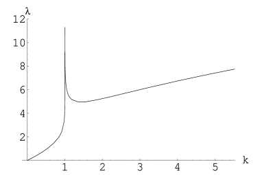
Figure 2: Wavelength $\lambda$ of the solutions as a function of $k$.

1.1 Domain wall solutions

For $k$ close to the critical value $k_{c}=1$ the solutions exhibit well separated wall-like structures. To illustrate this, we show in Fig.(3) a numerical solution $\phi(x)$ of Class IA subject to the initial condition ${\rm Re}\left[\phi(0)\right]=0.0001$ and ${\rm Im}\left[\phi(0)\right]=0$. The value of the “constant of the motion” $k$ that is associated with this solution is $k\approx 1-10^{-8}$. The corresponding energy-density $\varepsilon(x)$ is also indicated. It is clear that if the trajectory of the solution in the complex $\phi$ plane passes the supersymmetric vacuum at the origin, the ratio of the width of the walls to distance between them is small since the force driving the trajectory away from the minimum is small. In Fig.(4) a numerical solution, belonging to Class II and subject to the initial condition ${\rm Re}\left[\phi(0)\right]=0$ and ${\rm Im}\left[\phi(0)\right]=0.0001$, is shown. The value of the “constant of the motion” $k$ that is associated with this solution is $k\approx 1+10^{-8}$. For $k\uparrow 1$ the solution consists of equally spaced “right” walls (Class IA) or equally spaced “left” walls (Class IB), and for $k\downarrow 1$ the solution consists of equally spaced, alternating “left” and “right” walls. As the critical value $k_{c}=1$ is approached, the distance between the walls increases, but the width and the shape of the walls converge.

Figure 3: Numerical solution to the BPS equation of Class IA subject to the initial condition ${\rm Re}\left[\phi(0)\right]=0.0001$ and ${\rm Im}\left[\phi(0)\right]=0$. Depicted are (a) the real part of $\phi(x)$, (b) the imaginary part of $\phi(x)$, and (c) the energy density $\epsilon(x)$.

Figure 4: Numerical solution to the BPS equation of Class II subject to the initial condition ${\rm Re}\left[\phi(0)\right]=0$ and ${\rm Im}\left[\phi(0)\right]=0.0001$. Depicted are (a) the real part of $\phi(x)$, (b) the imaginary part of $\phi(x)$, and (c) the energy density $\epsilon(x)$.

1.2 Approximate solutions in between the walls

In between the walls, both the real and the imaginary part of $\phi$ are very small. In this region the trajectory is approximately governed by the BPS equation linearized about $\phi=0$

$$\frac{d\phi_{1}}{dx} = -2\phi_{2}\ ,$$

$$\frac{d\phi_{2}}{dx} = -2\phi_{1}\ .$$ (9)

The general solution of Eq. (1.2) is

$$\phi_{1}(x)=C_{+}e^{2x}+C_{-}e^{-2x}\ ,\ \ \ \phi_{2}(x)=-C_{+}e^{2x}+C_{-}e^{-2x}\ .$$ (10)

For Class I cycles, with the initial condition $\phi_{1}(0)=u$ and $\phi_{2}(0)=0$, the solution is

$$\phi_{1}(x)=u\cosh 2x\ ,$$

$$\phi_{2}(x)=-u\sinh 2x\ .$$ (11)

The constant $u$, which is very small for well separated walls, is related to the constant of motion $k$ of the solution by $k=(1-u^{2}/2)^{2}$. The approximation breaks down when $x$ is so large that the magnitude of the fields $\phi_{1}$ and $\phi_{2}$ becomes of the order one. This happens at the location of the walls. The wavelength of the solution is therefore related to the constant $k$ by $\lambda=-1/2\ln(1-k)$ for $k\uparrow 1$.

Similarly, the approximate solution for Class II solutions in between a “left” wall and a “right” wall is given by

$$\phi_{1}(x) = -v\sinh 2x\ ,$$

$$\phi_{2}(x) = v\cosh 2x\ .$$ (12)

The constant $v$, which also has to be very small for well separated walls, is related to the constant of motion by $k=(1+v^{2}/2)^{2}$. From this approximate solution it follows that the wavelength of the Class II solution is related to the constant $k$ by $\lambda=-\ln(k-1)$ in the limit $k\downarrow 1$.

1.3 BPS domain walls on a circle

So far we have discussed generic periodic solutions to the BPS equation. Now we want to determine what BPS saturated configurations are possible on a compact space with given circumference $L$. It is clear that we have to select only those solutions in the total solution space for which the wavelength $\lambda$ fits an integer $N$ times on the circumference $L$. The allowed values of $k$ are thus the solutions of the equation $L=N\lambda(k)$, where the integer $N$ is a winding number that specifies how many times the solution winds around the poles when $x$ varies between $0$ and $L$. In Fig.(2) we show the period function $\lambda(k)$, which gives the wavelength of a solution as a function of $k$.

The simplest BPS configurations have winding number $N=1$; for any value of $L$ there is such a configuration of Class IA and Class IB, but only if $L>\lambda_{m}$ is there such a configuration of Class II. The tension $T\equiv 2\Delta W$ of the Class I configurations is equal to $T=4\pi$ while the tension of the Class II configuration is equal to $T=8\pi$. When $L$ is very large, the Class IA and IB configuration describe just one “right” wall and one “left” wall, respectively. The Class II configuration contains one “right” wall and one “left” wall at a distance of $L/2$.

Similar considerations apply to configurations with higher winding number $N$. The tension of the BPS configurations is proportional to $N$. As long as $L$ is much larger than $N$ times the width of the walls, the configurations contain well separated equidistant domain walls, $N$ “right” (“left”) walls in Class IA (Class IB) configurations, and $N$ “left” walls alternating with $N$ “right” walls in Class II configurations.

1.4 Non-BPS domain walls

As explained in the previous section there is no Class II BPS saturated configuration if the circumference $L$ of the compact dimension is smaller than $\lambda_{m}$. However, there is a stable, static solution to the second order equations of motion with the same topology. Such a solution can not be BPS saturated. It is a non-contractable cycle, so it can not be shrunk to a point. At the same time it has to remain at finite distance of the origin in the complex $\phi$ plane because for fixed circumference $L$ the kinetic energy grows if the length of the trajectory in the complex $\phi$ plane increases.

Following the same argument, it is easy to see that there are stable, static configurations that are not BPS saturated in all other topological sectors. The simplest example is the homotopy class of non-contractable cycles which wind first clockwise around one pole and then counterclockwise around the other pole (”race-track” topology). With obvious notation, we will refer to these topologies as $RL^{-1}$ and $LR^{-1}$.

Summarizing, in any non-trivial topological sector and for any value of $L$ there is at least one static, stable solution to the second order equation of motion with minimal energy in that sector, a classical ground state. In certain topological sectors, those with the topologies $R^{N}$, $L^{N}$, $(R^{-1})^{N}$ and $(L^{-1})^{N}$, the stable solution is BPS saturated for any value of $L$, and only half of supersymmetry is broken in the classical ground state. In other topological sectors, those with the topologies $(RL)^{N}$ and $(R^{-1}L^{-1})^{N}$, there are two stable solutions that are BPS saturated if the circumference $L$ of the compact dimension is larger than a minimum value, $N\lambda_{m}$. If $L$ is smaller than the minimum value, then there is still a static solution to the equation of motion, but it is not BPS saturated.

2 d=3+1; localized light modes

In this section we study the massless and light modes in a BPS saturated background that takes the form of a sequence of equidistant domain walls. We have discussed configurations of this type in Section 1. As only half of supersymmetry is spontaneously broken, the theory of the massless and light modes in $d=2+1$ dimensions has ${\cal N}=1$ supersymmetry. We will therefore focus on the study of bosonic modes; clearly, each bosonic mode is accompanied by a fermionic mode that completes the supersymmetry multiplet.

There is an exact bosonic zero mode originating from the invariance of the action under translations along the compact dimension of the BPS saturated background as a whole. We will now study the spectrum of the bosonic pseudo zero modes corresponding to independent translations of the domain walls.

2.1 Tight binding approach

In oder to get a more quantitative picture of the bosonic pseudo zero modes, we follow Ref. [13] and expand the action in fluctuations of the fields around the classical, BPS saturated background configuration up to quadratic order. In contrast to the case of a real wall background as it was investigated in Ref. [13], we have to keep track of the fact that here the BPS saturated wall $\phi_{w}$ is complex. Writing $\phi=\phi_{w}+\phi^{\prime}$ and $\phi^{\prime}=\frac{1}{\sqrt{2}}(\phi_{1}^{\prime}+\imath\phi_{2}^{\prime})$ with real fields $\phi_{1}^{\prime}$ and $\phi_{2}^{\prime}$, the following equations of motion are obtained

$$\left(\partial_{\mu}\partial^{\mu}+\bar{W}^{\prime\prime}W^{\prime\prime}+\mbox{Re}\left[\bar{W}^{\prime}W^{\prime\prime\prime}\right]\right)\phi_{1}^{\prime}-\mbox{Im}\left[\bar{W}^{\prime}W^{\prime\prime\prime}\right]\phi_{2}^{\prime} = 0\ ,$$

$$\left(\partial_{\mu}\partial^{\mu}+\bar{W}^{\prime\prime}W^{\prime\prime}-\mbox{Re}\left[\bar{W}^{\prime}W^{\prime\prime\prime}\right]\right)\phi_{2}^{\prime}-\mbox{Im}\left[\bar{W}^{\prime}W^{\prime\prime\prime}\right]\phi_{1}^{\prime} = 0\ .$$ (13)

The primes denote derivatives with respect to $\phi$ ($\bar{\phi}$) in the case of $W$ ($\bar{W}$) evaluated at $\phi=\phi_{w}$ ($\bar{\phi}=\bar{\phi}_{w}$). For localized massless and massive modes we make the following decomposition

$$\phi_{1}^{\prime}=\chi_{1}(z)A(t,x,y)\ ,\ \ \ \phi_{2}^{\prime}=\chi_{2}(z)A(t,x,y)\ ,$$ (14)

where $\chi_{i}$ and $A$ are real fields. From the equation of motion, Eq.(2.1), we obtain the following equations of motion for these fields

$$-\frac{\partial_{n}\partial^{n}A}{A}=\frac{\left(-\partial^{2}_{z}+\bar{W}^{\prime\prime}W^{\prime\prime}+\mbox{Re}\left[\bar{W}^{\prime}W^{\prime\prime\prime}\right]\right)\chi_{1}-\mbox{Im}\left[\bar{W}^{\prime}W^{\prime\prime\prime}\right]\chi_{2}}{\chi_{1}}\equiv m^{2}\ ,$$

$$-\frac{\partial_{n}\partial^{n}A}{A}=\frac{\left(-\partial^{2}_{z}+\bar{W}^{\prime\prime}W^{\prime\prime}-\mbox{Re}\left[\bar{W}^{\prime}W^{\prime\prime\prime}\right]\right)\chi_{2}-\mbox{Im}\left[\bar{W}^{\prime}W^{\prime\prime\prime}\right]\chi_{1}}{\chi_{2}}\equiv m^{2}\ ,$$ (15)

where $n=0,1,2$ is a Lorentz index in $d=2+1$ dimensions. Hence, the field $A(t,x,y)$ has a mass $m$ in $d=2+1$ dimensions. The vector

$$\vec{\chi}\equiv\left(\begin{array}[]{c}\chi_{1}\\ \chi_{2}\end{array}\right),$$ (16)

satisfies the eigenvalue equation

$$H\vec{\chi}=m^{2}\vec{\chi}\ ,$$ (17)

where the hermitian operator $H$ is defined as

$$H=\left(\begin{array}[]{cc}-\partial_{z}^{2}+\bar{W}^{\prime\prime}W^{\prime\prime}+\mbox{Re}\left[\bar{W}^{\prime}W^{\prime\prime\prime}\right]&-\mbox{Im}\left[\bar{W}^{\prime}W^{\prime\prime\prime}\right]\\ -\mbox{Im}\left[\bar{W}^{\prime}W^{\prime\prime\prime}\right]&-\partial_{z}^{2}+\bar{W}^{\prime\prime}W^{\prime\prime}-\mbox{Re}\left[\bar{W}^{\prime}W^{\prime\prime\prime}\right]\end{array}\right)\ .$$ (18)

This equation has the form of a one-dimensional Schrödinger equation, and, in analogy, we will refer to $H$ as the Hamiltonian and to $\vec{\chi}$ as the wave function. Using the BPS equation, Eq. (7), it is not difficult to explicitly show that $H$ annihilates $\chi=\partial_{z}\phi_{w}$, which corresponds to the Goldstone boson of spontaneously broken overall translational invariance along the $\hat{z}$ direction.

Since we are not able to solve the eigenvalue problem in Eq.(17) exactly, we resort to the tight binding approximation to study the masses of the pseudo zero modes corresponding to independent translations of the individual walls. For definiteness, we take the $R^{N}$ topological sector, with the background of $N$ walls separated by a distance $\lambda=L/N$. Considerations for the $(RL)^{N}$ sectors are similar, but slightly more complicated due to the sequence of alternating walls and anti-walls. We will uncover the light bosonic modes of the wall lattice by first considering a massless mode bound to a single wall in isolation, just as one can find the electronic levels of a one dimensional crystal from the energy levels of the individual atoms when they are far apart and overlaps are small.

Thus, we consider a single wall, $\phi_{c}^{w}$, along an infinite dimension. In this limit $\chi^{0}\equiv\frac{1}{\sqrt{2\pi}}\partial_{z}\phi_{c}^{w}$ is a normalized eigen function with $m^{2}=0$. In the case of $N$ such walls separated by an infinite distance, there are $N$ localized (bound) wave functions with vanishing mass. However, when the walls are at a large, but finite, distance from each other, the $N$-fold degeneracy is lifted due to the small overlap of potentials and wave functions centered at different wall sites, and a band structure emerges. We will now elucidate this band structure, and we will estimate the width of the band.

To this end we decompose the operator $H^{c}=H^{0}+V^{c}$, where

$$H^{0}=\left(\begin{array}[]{cc}-\partial_{z}^{2}+4&0\\ 0&-\partial_{z}^{2}+4\end{array}\right),$$ (19)

and

$$V^{c}=\left(\begin{array}[]{cc}\bar{W}_{c}^{\prime\prime}W_{c}^{\prime\prime}-4+\mbox{Re}\left[\bar{W}_{c}^{\prime}W_{c}^{\prime\prime\prime}\right]&-\mbox{Im}\left[\bar{W}_{c}^{\prime}W_{c}^{\prime\prime\prime}\right]\\ -\mbox{Im}\left[\bar{W}_{c}^{\prime}W_{c}^{\prime\prime\prime}\right]&\bar{W}_{c}^{\prime\prime}W_{c}^{\prime\prime}-4-\mbox{Re}\left[\bar{W}_{c}^{\prime}W_{c}^{\prime\prime\prime}\right]\end{array}\right).$$ (20)

Here the superscript $c$ indicates that the quantity is evaluated at $\phi=\phi_{c}^{w}$. With this definition, $V^{c}$ vanishes exponentially fast away from the wall. We approximate $H$ in the case of $N$ walls separated by a distance $\lambda$ as

$$H=H^{0}+\sum_{n}V^{c}(z-n\lambda).$$ (21)

This Hamiltonian commutes with the generator of the $R_{N}$ symmetry, the translations over distances $n\lambda$. The (pseudo zero mode) wave functions, the equivalent of Bloch waves, are linear combinations of $\vec{\chi^{0}}$ centered at each of the $N$ wall sites. These linear combinations transform under irreducible representations of $R_{N}$. They take the form

$$\vec{\chi}_{k}=\sum_{n}a_{k}\left[n\right]\vec{\chi}^{0}(z-n\lambda),$$ (22)

where $\vec{a}_{k}$, with $k=1..N$, are the $N$ real, orthonormal eigenvectors of the $N\times N$ matrix

$$\left(\begin{array}[]{ccccccccc}2&-1&0&.&.&.&.&0&-1\\ -1&2&-1&0&.&.&.&.&0\\ 0&-1&2&-1&0&.&.&.&0\\ .&.&.&.&.&.&.&.&.\\ 0&.&.&.&.&0&-1&2&-1\\ -1&0&.&.&.&.&0&-1&2\end{array}\right).$$ (23)

This matrix has a non-degenerate eigenvalue equal to zero for any value of $N$, with eigenvector $\vec{a}_{1}=\frac{1}{\sqrt{N}}(1,1,..,1)$. For even values of $N$ there is a second non-degenerate eigenvalue equal to $4$ with eigen vector $\vec{a}_{2}=\frac{1}{\sqrt{N}}(1,-1,1,..,-1,1)$. All other eigenvalues are between $0$ and $4$ and are doubly degenerate. Therefore, the $N$ dimensional representation of $R_{N}$ is reduced to $2$ one-dimensional and $N/2-1$ two-dimensional irreducible representations in case $N$ is even, and to $1$ one-dimensional and $(N-1)/2$ two-dimensional irreducible representations in case $N$ is odd.

As an aside, the eigenvectors and eigenvalues of the matrix in Eq.(23) also yield the normal modes and frequencies of a closed linear chain of $N$ identical masses and springs. In $d=3+1$ dimensions, the walls extend into two infinite dimensions and have therefore infinite mass. However, for solitons in $d=1+1$ dimensions, which have finite energy, these vibrations are physical. If the distance between the solitons is large as compared to their width, these vibrations are very soft.

Given the wave functions in Eq.(22), the approximate mass eigenvalues are then given by

$$m_{TB}^{2}=\frac{\int_{0}^{L}dz\vec{\chi}^{T}\,H\,\vec{\chi}}{\int_{0}^{L}dz\vec{\chi}^{T}\vec{\chi}}.$$ (24)

In fact, for the wave functions that transform under the two dimensional representation of $R_{N}$, degenerate perturbation theory should be used. Including only overlap integrals from neighboring sites, and using the asymptotic form for $\vec{\chi}^{c}$ far away from the wall, we estimate that the masses are exponentially suppressed,

$$m_{TB}^{2}=Ce^{-2\lambda},$$ (25)

where $C$ is of the order one. We thus see that the $N$ degenerate vanishing masses in the limit where the walls are infinitely far apart evolve into a (mostly double degenerate) band of masses when the distance between the walls becomes finite.

2.2 Oscillations

For an observer who can not resolve the circumference $L$ of the compact dimension, the physics of the light modes is described by an ${\cal N}=1$ supersymmetric theory in $d=2+1$ dimensions with a spectrum as we discussed in the previous section. In such a world there is a hierarchy between the heavy modes, with masses comparable to the wall tension, and the light modes, with masses that are exponentially suppressed by the ratio of the distance between the walls and their width. It is interesting to note that in topological sectors with multi-wall backgrounds that are not BPS saturated the physics of the light modes is described by a ${\cal N}=1$ model with supersymmetry breaking. The scale of the breaking is equal to the scale of the light masses. It seems that under such conditions there are no hierarchy or naturalness problems.

Alternatively, an observer, who is confined to a particular wall and can not resolve its width, experiences a different physical reality. Such an observer does not have the means to do experiments in which the massive bulk modes are excited. Still, due to the BPS saturation of the background, his world has ${\cal N}=1$ supersymmetry. But he will be perplexed by the appearance and disappearance of particles in his world. From the ansatz of Eq. (22) it is clear that a state localized on a particular wall must be a superposition of the wave functions that represent the light modes. This in turn means that such a state is not a mass eigenstate. The implication is oscillation of localized particles between the various walls with frequencies corresponding to the mass differences. In the analogy of a linear crystal, this would correspond to electrons hopping from atom to atom. For example, in the case of the $R^{2}$ sector with two walls, the approximate massless mode is

$$\vec{\chi}_{1}(z)=\vec{\chi}^{0}(z)+\vec{\chi}^{0}(z-\lambda)\ ,\ \$$ (26)

and there is one light mode, approximately given by

$$\vec{\chi}_{2}(z)=\vec{\chi}^{0}(z)-\vec{\chi}^{0}(z-\lambda)\ .$$ (27)

A state localized one of the walls is constructed by the superposition of the mass eigenstates,

$$\vec{\chi}_{0}(z)\pm\vec{\chi}_{1}(z)\ .$$ (28)

3 d=2+1; chiral fermions

When the model is dimensionally reduced to $d=2+1$ dimensions, it has ${\cal N}=2$ supersymmetry. It has inherited four supersymmetry generators, whereas minimal supersymmetry in $d=2+1$ requires only two generators. The scalar potential may be written as

$$V=\sum_{i=1}^{2}\left(\frac{\partial{\cal W}}{\partial\phi_{i}}\right)^{2}.$$ (29)

The object $\cal W$ plays the role of the superpotential in the dimensionally reduced model. It is related to the superpotential $W$ in $d=3+1$ dimensions by

$${\cal W}=2{\rm Im}\left[W\left(\frac{1}{\sqrt{2}}(\phi_{1}+\imath\phi_{2})\right)\right]=2\arctan\frac{\phi_{2}}{\phi_{1}+\sqrt{2}}+2\arctan\frac{\phi_{2}}{\phi_{1}-\sqrt{2}}\,.$$ (30)

The extended supersymmetry manifests itself in the fact that the superpotential $\cal W$ is harmonic. In terms of the scalar components of the ${\cal N}=1$ superfields in $d=2+1$ dimensions, $\phi_{1}$ and $\phi_{2}$, the BPS equations are

$$\frac{d\phi_{1}}{dx} = \alpha\frac{\partial{\cal W}}{\partial\phi_{1}}=2\alpha\left\{-\frac{\phi_{2}}{(\phi_{1}+\sqrt{2})^{2}+\phi_{2}^{2}}-\frac{\phi_{2}}{(\phi_{1}-\sqrt{2})^{2}+\phi_{2}^{2}}\right\},$$

$$\frac{d\phi_{2}}{dx} = \alpha\frac{\partial{\cal W}}{\partial\phi_{2}}=2\alpha\left\{\frac{\phi_{1}+\sqrt{2}}{(\phi_{1}+\sqrt{2})^{2}+\phi_{2}^{2}}+\frac{\phi_{1}-\sqrt{2}}{(\phi_{1}-\sqrt{2})^{2}+\phi_{2}^{2}}\right\},$$ (31)

where $\alpha=\pm 1$. The interesting new feature in $d=2+1$ dimensions is that now “chiral” fermions exist on the $d=1+1$ dimensional worlds of the domain walls. In $d=1+1$ dimensions there is no spin, but massless fermions can be either left or right moving; this is what we will allude to as “chirality”. As outlined in the Appendix, in a BPS saturated background configuration there is always one left moving and one right moving fermionic zero mode, corresponding to the two spontaneously broken supersymmetry generators. Whether a mode that is associated with a particular broken generator is left or right moving depends on the sign $\alpha$ in the BPS equation that provides the background configuration. In other words, it is not important around which pole the background configuration winds in the complex $\phi$ plane, but whether it winds clockwise or counter clockwise.

3.1 Wess-Zumino model

In order to further investigate the issue of the “chirality” of massless fermions on the wall, we discuss in this section the regular Wess-Zumino model reduced to $d=2+1$ dimensions. It is well known that this model allows for real, BPS saturated domain walls (kink or anti-kink). However, these solutions do not exist in a compact dimension, and there are no BPS saturated multi-wall solutions (although almost static configurations with walls at large distances do exist). For the issues we want to discuss here, these differences are irrelevant.

Our analysis is similar to the discussion of fermionic zero modes in Ref.[19], where the same model was investigated in $d=1+1$ dimensions. The superpotential of the dimensionally reduced, regular Wess-Zumino model is

$${\cal W}=\frac{1}{\sqrt{2}}\left(2\phi_{1}-\frac{1}{3}\phi_{1}^{3}+\phi_{1}\phi_{2}^{2}\right).$$ (32)

There are two vacua, $\phi_{1}=\pm\sqrt{2}$ with $\phi_{2}=0$. The BPS saturated domain walls connecting these vacua are determined by

$$\frac{d\phi_{1}}{dy} = \alpha\frac{1}{\sqrt{2}}\left(2-\phi_{1}^{2}+\phi_{2}^{2}\right),$$

$$\frac{d\phi_{2}}{dy} = \alpha\frac{1}{\sqrt{2}}\left(2\phi_{1}\phi_{2}\right),$$ (33)

where $\alpha=\pm 1$. The solutions that interpolate between the two vacua (the well-known kink or anti-kink, depending on the sign $\alpha$), take the form

$$\phi_{1}^{w} = \alpha\sqrt{2}\tanh(x-x_{0})$$

$$\phi_{2}^{w} = 0.$$ (34)

The equation of motion for the fermions in the background is

$$\imath\gamma^{m}\partial_{m}\psi_{i}-{\bf W}_{ij}\psi_{j}=0\ ,$$ (35)

where the “mass” matrix ${\bf W}$ is given as

$${\bf W}=\sqrt{2}\left(\begin{array}[]{cc}-\phi_{1}^{w}&\phi_{2}^{w}\\ \phi_{2}^{w}&\phi_{1}^{w}\end{array}\right)\ .$$ (36)

There are two massless fermions on the wall corresponding to Rebbi–Jackiw zero modes,

$$\psi_{1}(x,y,t) = A(y)\zeta(x,t),$$

$$\psi_{2}(x,y,t) = 0\ ,$$ (37)

with

$$A(y) = e^{\alpha\int_{y_{0}}^{y}{\rm W}_{11}(y^{\prime})dy^{\prime}},$$

$$\imath\gamma^{2}\zeta = \alpha\zeta\ ,$$

and

$$\psi_{1}(x,y,t) = 0,$$

$$\psi_{2}(x,y,t) = B(y)\eta(x,t)\ ,$$ (38)

where

$$B(y) = e^{-\alpha\int_{y_{0}}^{y}{\rm W}_{22}(y^{\prime})dy^{\prime}},$$

$$\imath\gamma^{2}\eta = -\alpha\eta\ .$$

Both $\zeta$ and $\eta$ satisfy the massless Dirac equation in $d=1+1$ dimensions, $\imath\gamma^{a}\partial_{a}\zeta=0$, where $a=0,1$. Note that $\gamma^{2}$ is the chiral projection matrix in $d=1+1$ dimensions, so that one of the massless fermions is right moving and the other one is left moving. These massless fermions are the goldstino fermions associated with the breaking of two out of four generators of the ${\cal N}=2$ supersymmetry, as discussed in the Appendix.

We proceed by addressing the fate of these massless fermions when the ${\cal N}=2$ supersymmetry is explicitly broken to ${\cal N}=1$. In this case, the wall breaks one of the remaining two supersymmetry generators, and therefore only one Goldstone fermion exists. What happens to the second massless fermion when the explicit supersymmetry breaking is switched on? To answer this question we introduce explicit ${\cal N}=2$ breaking terms in the superpotential.

First, we insert a coupling constant $\lambda$ in front of the $\phi_{1}\phi_{2}^{2}$ term in the superpotential, so that the ${\cal N}=2$ supersymmetry is explicitly broken unless $\lambda=1$. The vacuum expectation values and the wall solution do not depend on $\lambda$, but ${\rm W}_{22}$ now is equal to $\lambda\phi_{1}^{w}$. Even though there is only one Goldstino, from the perspective of the Rebbi-Jackiw zero modes in Eqs. (37,38), it is clear that the second massless fermion continues to exist, even if $\lambda\neq 1$. When $\lambda$ changes sign, the second massless fermion changes from right to left moving (or vice versa, depending on the sign $\alpha$), and for $\lambda=0$ the second massless fermionic mode is not normalizable.

Next, we add a term $\frac{1}{2}\,\mu\phi_{2}^{2}$ to the superpotential, so that the ${\cal N}=2$ supersymmetry is explicitly broken to ${\cal N}=1$ for $\mu\neq 0$. Again, the vacuum expectation values and the wall do not depend on $\mu$, but now ${\rm W}_{22}=\phi_{1}^{w}+\mu$. In this case the second massless fermion persists as long as $|\mu|<\sqrt{2}$. For $|\mu|>\sqrt{2}$ the second zero mode becomes non-normalizable.

It is clear that since the fermionic modes on the wall are chiral, they can only become massive in pairs, combining one left moving and with one right moving fermion. Individual massless modes, either left or right moving, can only disappear when they become non-normalizable.

3.2 Complex, multi-wall backgrounds

In the case of a BPS saturated background with one domain wall along a compact dimension, there is one massless scalar localized on the wall corresponding to the spontaneously broken translational symmetry. Moreover, there is one left moving and one right moving massless fermion, corresponding to the two spontaneously broken supersymmetry generators (see the Appendix). These massless modes combine to form a massless superfield in $d=1+1$ dimensions.

The supersymmetry multiplet in $d=1+1$ dimensions contains a real scalar and a Majorana fermion. Therefore, in the case of $N$ walls, there will be a total of $N-1$ light superfields ($d=1+1$, ${\cal N}=1$ supersymmetry) with exponentially suppressed masses, and one massless superfield. In order to make states localized on a particular wall, states with different masses have to be superimposed, just as in the $d=3+1$ dimensional case.

The explicit analysis of the Rebbi–Jackiw modes becomes impossible if the fermion “mass” matrix in the background is not diagonal, as is the case with the type of models we consider in this paper. But the results of the previous section must still be valid. It is therefore expected that if the ${\cal N}=2$ supersymmetry is explicitly broken to ${\cal N}=1$, there will still be a left and a right moving fermion on the wall, at least for a finite range of the breaking parameters. Moreover, in a compact dimension, it seems unlikely that fermionic zero modes can disappear by becoming non-normalizable.

4 d=1+1; solitons

The main new feature in $d=1+1$ dimensions is that the domain walls, which have infinite energy in higher dimensions, now reduce to solitons with a finite mass. Such solitons have a particle interpretation, whereas the domain wall backgrounds in the higher dimensions are interpreted as vacua.

All topological sectors in the $d=1+1$ dimensional theory, whether they have a BPS saturated ground state or not, can be assigned a pair of winding numbers $(N_{l},N_{r})$, where $N_{l}\in{\bf Z}$ is the winding number around the “left” pole at $\phi=-1$ in Fig.(1), and $N_{r}\in{\bf Z}$ is the winding number around the “right” pole at $\phi=+1$. According to our conventions the winding number increases by one if a pole is encircled in the counter clockwise direction. This classification of the sectors according to the pair of winding numbers is not unique; for example, the sectors $RLRL^{-1}$ and $R^{2}$ have the same winding numbers, $(0,2)$, but they are topologically distinct.

The sectors $L^{N_{l}}$ and $R^{N_{r}}$ have a classical ground state in which only half of supersymmetry is broken for any value of $L$. In the $L^{N_{l}}$ sector this ground state corresponds to the solution of the BPS equation which in the large $L$ limit contains $N_{l}$ “left” solitons if $N_{l}$ is positive, or $|N_{l}|$ anti “left” solitons if $N_{l}$ is negative, separated by a distance $L/|N_{l}|$. The situation is analogous for the $R^{N_{r}}$ sectors.

For fixed $L>\lambda_{m}$, the sectors $(RL)^{N}$ have two degenerate classical ground states in which only half of supersymmetry is broken. In the large $L$ limit, and if $N$ is positive, one of these ground states corresponds to the solution of the BPS equation containing $N$ “left” solitons which alternate with $N$ “right” solitons, separated by a distance $L/2N$. Similarly, if $N$ is negative we have the BPS solution with $|N|$ “anti-left” solitons alternating with $|N|$ “anti-right” solitons separated by a distance $L/2N$. The second, degenerated ground state corresponds to the BPS solution that winds around both poles at large distance, $N$ times in the counterclockwise direction if $N$ is positive, and $|N|$ times in the clockwise direction if $N$ is negative. This solution to the BPS equation has approximately constant energy density in the large $L$ limit. There is a tunneling transition with finite action that connects the two ground states and the remaining $1/2$ of supersymmetry is broken non-perturbatively. For $L<N\lambda_{m}$, there is no BPS saturated ground state in the sector $(RL)^{N}$ already at the classical level. There are static, stable solutions to the second order equation of motion which break supersymmetry completely at the classical level.

For the same reason, supersymmetry is broken completely in the groundstate at the classical level in all sectors other than the ones we discussed above. In all sectors, the ground state energy tends to $2\pi(|N_{l}|+|N_{r}|)$ in the large $L$ limit. The theory has two types of solitons, “left” and “right”, and two topologically conserved quantum numbers, $N_{l}$ and $N_{r}$. The solitons interact through a short range force, which decreases exponentially with distance. “Left” and “right” solitons repel each other, and so do “anti-left” and “anti-right” solitons. “Left” and “anti-left” solitons on the other hand attract each other.

4.1 Semi-classical calculation of the tunneling amplitude

In this section we calculate the amount by which the ground state energy is lifted above the BPS bound by the tunneling transition in the sector $(RL)^{N}$, for $N=1$ and $L>\lambda_{m}$. We choose $N=1$ for definiteness; the tunneling action scales linearly with $|N|$, and therefore the result can be trivially generalized for any value of $N$. The two ground states correspond to two solutions of the BPS equation in Class II, one with $k<k_{m}$ and one with $k>k_{m}$, as shown in Fig.(5). At the non-perturbative level the corresponding solitons are not longer BPS saturated because a tunneling process mixes them and lifts their mass above the BPS bound. This phenomenon was first observed in Ref.[20]. In Ref.[21] it was noted that the calculation of the semi-classical instanton action is equivalent to the calculation of the energy of domain wall junctions in $d=2+1$ dimensions. In the same work, the general calculational framework of the action was established and illustrated for a specific model.

We assume that the instanton in the imaginary time saturates the BPS bound in the model we consider; there is no obvious reason why this would not be the case. If the instanton is BPS saturated, it satisfies the equation

$$\frac{\partial\phi}{\partial\zeta}=\frac{1}{2}e^{i\delta}\frac{d\bar{W}}{d\bar{\phi}},$$ (39)

where $\zeta=x+it$, and $t$ is the euclidean time. The field $\phi$ depends both on $\zeta$ and $\bar{\zeta}$. The phase $\delta$ has to be chosen so that it is consistent with the boundary conditions that are imposed on the solution (see below). The tunneling action takes the form

$$A = 2\int dxdt\left\{\frac{\partial\phi}{\partial\zeta}\frac{\partial\bar{\phi}}{\partial\bar{\zeta}}+\frac{\partial\phi}{\partial\bar{\zeta}}\frac{\partial\bar{\phi}}{\partial\zeta}\right\}$$ (40)

$$+\int dxdt\frac{dW}{d\phi}\frac{d\bar{W}}{d\bar{\phi}}.$$

In Figs.(5, 6) we have indicated the boundary conditions that are imposed on the instanton configuration. At $t=-T/2$ the instanton field $\phi(x,t)$ takes the form of the “outer” configuration (see Fig.(5)) and at $t=T/2$ it takes the form of the “inner” configuration. We always have in mind the limit $T\rightarrow\infty$. Periodic boundary conditions apply to the vertical edges in Fig.(6).

Figure 5: The initial (outer) and final (inner) configurations in the complex $\phi$ plane. Both configurations are solutions to the BPS equation with the same wavelength $\lambda$. The instanton interpolates smoothly between the initial and final configuration with finite action.

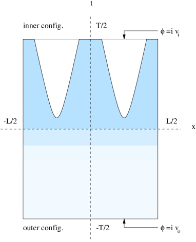
Figure 6: Boundary conditions in the $x$-$t$ plane. The initial and final configuration at the bottom ($-T/2$) and top ($T/2$) of the rectangle are traced counter-clockwise in the complex $\phi$ plane (see Fig.(5)). Periodic boundary conditions apply to the vertical edges. The shading schematically indicates the energy density, with the darker areas indicating higher energy density.

We have chosen the solutions to wind counter-clockwise in the $\phi_{1}$-$\phi_{2}$ plane when followed in the positive $\hat{x}$ direction, which corresponds to $\delta=\pi/2$ in the BPS equation. The initial and final configuration are positioned such that $\phi(L/2,-T/4)=iv_{0}$ and $\phi(L/2,T/4)=iv_{i}$. Note that in order for the instanton configuration to satisfy the BPS equation, it has to connect the solution with the larger value of $k$ as the initial configuration with the solution with the smaller value of $k$ as the final configuration. The anti-instanton that interpolates in the reverse situation satisfies an anti-BPS equation. The action can now be written as

$$A_{BPS}=\int dxdt\,\left[2\vec{\nabla}\cdot\vec{S}-(\vec{\nabla}\times\vec{a})_{z}\right],$$ (41)

where

$$\vec{S}=\left(\begin{array}[]{c}\cos\delta\,{\rm Re}\left[W\right]+\sin\delta\,{\rm Im}\left[W\right]\\ \cos\delta\,{\rm Im}\left[W\right]-\sin\delta\,{\rm Re}\left[W\right]\\ \end{array}\right),$$ (42)

and

$$\vec{a}=\left(\begin{array}[]{c}{\rm Im}\left[\phi\frac{\partial\bar{\phi}}{\partial x}\right]\\ {\rm Im}\left[\phi\frac{\partial\bar{\phi}}{\partial t}\right]\\ \end{array}\right).$$ (43)

With the application of Gauss’ and Stoke’s theorems the surface integrals can be converted into line integrals over the boundaries of the surface,

$$A_{BPS}=2\oint\vec{S}\cdot d\vec{n}-\oint\vec{a}\cdot d\vec{x},$$ (44)

where the boundaries are the edges of the rectangle in Fig.(6). Due to the periodic boundary conditions only the integrals of $\vec{S}$ contribute over the vertical edges of the contour, as the superpotential is multi-valued. Turning now to the explicit calculation of the tunneling action, there are three non-vanishing contributions. First, consider

$$A_{BPS}^{0} = 2\int_{-T/2}^{T/2}\left\{{\rm Im}\left[W\right]_{x=\frac{L}{2}}-{\rm Im}\left[W\right]_{x=-\frac{L}{2}}\right\}dt,$$ (45)

$$= 8\pi T.$$

This contribution is equal to the classical ground state energy times the elapsed time $T$. It is equal to the action in case there is no tunneling, when the initial and final configuration are the same. We define the tunneling probability by subtracting this trivial contribution in the exponent. Next, consider

$$A_{BPS}^{1} = 2\int_{-L/2}^{L/2}\left\{{\rm Re}\left[W\right]_{t=-\frac{T}{2}}-{\rm Re}\left[W\right]_{t=\frac{T}{2}}\right\}dx$$ (46)

$$= \ln\left(\frac{k_{0}}{k_{i}}\right)L,$$

where $k_{o}$ and $k_{i}$ are the two solutions to the equation $\lambda(k)=L$ with $k>k_{c}$. We define $k_{o}$ to be the larger of the two. Note that the integrands are “constants of motion” for the solutions to the BPS equation, and therefore the integrals can be expressed in $k_{o}$ and $k_{i}$, respectively. In the limit $\lambda=L\gg\lambda_{m}$, $k_{i}$ approaches $1$ from above, and $k_{o}$ is related to $L$ by $L=\pi\sqrt{k}$. In this limit, the second contribution to the tunneling action is therefore $A_{BPS}^{1}=2L\ln L/\pi$. Finally, we calculate

$$A_{BPS}^{2} = \int\left\{{\rm Im}\left[\phi\frac{\partial\bar{\phi}}{\partial x}\right]_{t=-\frac{T}{2}}-{\rm Im}\left[\phi\frac{\partial\bar{\phi}}{\partial x}\right]_{t=\frac{T}{2}}\right\}dx$$ (47)

$$= -S(k_{o})+S(k_{i}),$$

where $S(k)$ is the area enclosed in the $\phi_{1}$-$\phi_{2}$ plane by the solution to the BPS equation marked by $k$. $S(k)$ is a monotonically increasing function of $k$. In the limit $k\downarrow k_{c}=1$, $S(k)$ approaches $S(1)=4$ from above. For large values of $k$ on the other hand $S(k)=2\pi\sqrt{k}$. Therefore, in the limit $\lambda=L\gg\lambda_{m}$, the third contribution to the tunneling action is approximately $A_{BPS}^{2}=-2\pi\sqrt{k_{o}}+1$, or, in terms of $L$, $A_{BPS}^{2}=-2L+1$.

We have calculated the tunneling action solely in terms of quantities related to the boundary configurations. An explicit interpolating instanton configuration is not needed, just the existence of a BPS saturated instanton configuration is sufficient. In the large $L$ limit, the semi-classical approximation is valid, and the ground state energy is lifted above the BPS bound by an amount

$$\Delta E\propto 8\pi e^{2A_{BPS}}=8\pi\,e^{-4L\ln L},$$ (48)

to leading order in $L$. The solution to the BPS equation that connects the vacuum at $\phi=0$ to the runaway vacuum at $\phi\rightarrow i\infty$ (this is a solution that is not periodic, obtained with $\delta=0$) has infinite tension. The circumference $L$ in a sense acts like an infra-red regulator. For this reason, the tunneling action is not linear in $L$, but proportional to $L\ln L$. We also note that in this model the instanton mixes a state containing two localized solitons with a state that corresponds to a flat energy density. This is in contrast with the model considered in Ref.[21], where the mixing is between two states with different solitons.

Summary

We have constructed a toy model to study some issues related to the idea of “brane worlds” in a field theoretical context. This toy model is a simple Wess-Zumino model with only one chiral superfield in $d=3+1$ dimensions. Different aspects were studied in various dimensions.

We showed that it is possible to have BPS saturated configurations with multiple, well separated domain walls in a compact space dimension. Generically, in such a background there are light modes with masses exponentially suppressed by the ratio of the distance between the walls and their width. These modes form the “matter” of the “brane world”, wheras the domain walls play the role of branes in our simple picture. We also described how particles can oscillate between walls. We illustrated these issues in our specific model.

We also found that the “chiral” fermions localized on $d=1+1$ dimensional BPS saturated walls embedded in a $d=2+1$ dimensional space-time always come in pairs; one is left moving, and one is right moving.

Finally, we discussed the toy model in $d=1+1$ dimensions. The domain walls then reduce to solitons with a finite mass. We showed that some classically BPS saturated states are lifted non-perturbatively by instanton tunneling.

Appendix A

In this Appendix we establish our notation and discuss the zero modes in a BPS saturated background.

d=3+1 dimensions

We use the conventions outlined in [13]. The signature of the metric $g^{\mu\nu}$ is $(+,-,-,-)$. The component Lagrangian for an ${\cal N}=1$ Wess-Zumino model in $d=3+1$ dimensions with canonical Kähler potential and superpotential $W$ is

$$\cal{L} = \partial_{\mu}\bar{\phi}\partial^{\mu}\phi+\imath\psi^{\alpha}\sigma_{\alpha\dot{\alpha}}^{\mu}\partial_{\mu}\bar{\psi}^{\dot{\alpha}}+F^{\dagger}F$$ (49)

$$+F\frac{dW}{d\phi}-\frac{1}{2}\frac{d^{2}W}{d\phi^{2}}\psi^{\alpha}\psi_{\alpha}$$

$$+\bar{F}\frac{d\bar{W}}{d\bar{\phi}}-\frac{1}{2}\frac{d^{2}\bar{W}}{d^{2}\bar{\phi}}\bar{\psi}_{\dot{\alpha}}\bar{\psi}^{\dot{\alpha}}.$$

The component fields transform under the supersymmetry transformations as

$$\delta\phi = \zeta^{\alpha}\psi_{\alpha},$$

$$\delta\psi_{\alpha} = \imath\sigma_{\alpha\dot{\alpha}}^{\mu}\bar{\zeta}^{\dot{\alpha}}\partial_{\mu}\phi+\zeta_{\alpha}F,$$

$$\delta F = \imath\bar{\zeta}_{\dot{\alpha}}\bar{\sigma}^{\mu\dot{\alpha}\alpha}\partial_{\mu}\psi_{\alpha},$$ (50)

where the transformation parameter $\zeta$ is the two component complex Grassmann variable. The auxiliary field $F$ can be eliminated by the use of its equation of motion $\bar{F}=-\frac{d\bar{W}}{d\bar{\phi}}$ to give the Lagrangian density

$$\cal{L} = \partial_{\mu}\bar{\phi}\partial^{\mu}\phi+\imath\psi^{\alpha}\sigma_{\alpha\dot{\alpha}}^{\mu}\partial_{\mu}\bar{\psi}^{\dot{\alpha}}-\frac{dW}{d\phi}\frac{d\bar{W}}{d\bar{\phi}}$$ (51)

$$-\frac{1}{2}\frac{d^{2}W}{d\phi^{2}}\psi^{\alpha}\psi_{\alpha}-\frac{1}{2}\frac{d^{2}\bar{W}}{d\bar{\phi}^{2}}\bar{\psi}_{\dot{\alpha}}\bar{\psi}^{\dot{\alpha}}.$$

The BPS equation for domain walls reads

$$\frac{d\phi}{dz}=e^{\imath\delta}\frac{d\bar{W}}{d\bar{\phi}},$$ (52)

where in a non-compact direction the phase $\delta$ is determined from the equation

$${\rm Im}\left[e^{-\imath\delta}W(\phi(z=-\infty)\right]={\rm Im}\left[e^{-\imath\delta}W(\phi(z=+\infty)\right].$$ (53)

BPS domain walls in a compact dimension are only possible if the superpotential is not single valued. In the models we consider $e^{\imath\delta}\pm i$.

Let us now expand the Lagrangian of the model about the non-trivial solution $\phi_{w}$ of the BPS equation. Setting $\phi=\phi_{w}+\phi^{\prime}$ and expanding up to quadratic terms in the fluctuations $\phi^{\prime}$, we obtain

$${\cal L} = \partial_{\mu}\bar{\phi}\partial^{\mu}\phi+\imath\psi^{\alpha}\sigma_{\alpha\dot{\alpha}}^{\mu}\partial_{\mu}\bar{\psi}^{\dot{\alpha}}$$ (54)

$$-\frac{1}{2}\left\{W^{\prime\prime\prime}\bar{W}^{\prime}\phi^{\prime 2}+W^{\prime}\bar{W}^{\prime\prime\prime}\bar{\phi}^{\prime 2}+2W^{\prime\prime}\bar{W}^{\prime\prime}\phi^{\prime}\bar{\phi}^{\prime}+W^{\prime\prime}\psi^{\alpha}\psi_{\alpha}+\bar{W}^{\prime\prime}\bar{\psi}_{\dot{\alpha}}\bar{\psi}^{\dot{\alpha}}\right\},$$

where the primes on $W$ ($\bar{W}$) indicate derivatives with respect to $\phi$ ($\bar{\phi}$) evaluated at $\phi=\phi_{w}$ ($\bar{\phi}=\bar{\phi}_{w}$). The equation of motion for the scalar in the wall background is

$$\partial^{2}\phi^{\prime}+\left\{W^{\prime}\bar{W}^{\prime\prime\prime}\bar{\phi}^{\prime}+W^{\prime\prime}\bar{W}^{\prime\prime}\phi^{\prime}\right\}=0,$$ (55)

and the equation of motion for the fermion in the wall background is

$$\imath\sigma_{\alpha\dot{\alpha}}^{\mu}\partial_{\mu}\bar{\psi}^{\dot{\alpha}}-W^{\prime\prime}\psi_{\alpha}=0.$$ (56)

Half of the supersymmetry generators is broken by the wall solution. In order to determine which generators are unbroken, we act with the SUSY generators on the wall and find

$$\delta\psi_{\alpha}=-\frac{1}{\alpha}\frac{d\phi_{w}}{dz}\left(\zeta_{\alpha}+\imath\alpha\sigma_{\alpha\dot{\alpha}}^{3}\bar{\zeta}^{\dot{\alpha}}\right),$$ (57)

where we have used the BPS equation, and $\alpha=\pm 1$. Transformations, for which the parameter satisfies $\zeta_{\alpha}=\imath\alpha\sigma_{\alpha\dot{\alpha}}^{3}\bar{\zeta}^{\dot{\alpha}}$, correspond to unbroken symmetries. The massless fermions localized on the wall which are related to the broken SUSY generators take the form

$$\psi_{\alpha}(x,y,z,t)=-\frac{d\phi_{w}}{dz}(z)\zeta_{\alpha}(x,y,t),$$ (58)

where $\zeta_{\alpha}(x,y,t)$ is constrained by

$$\zeta_{\alpha}=+\imath\alpha\sigma_{\alpha\dot{\alpha}}^{3}\bar{\zeta}^{\dot{\alpha}}.$$ (59)

It can then be verified that $\psi_{\alpha}$ satisfies the fermionic equation of motion in the domain wall background if $\zeta_{\alpha}$ satisfies the equation

$$\imath\sigma_{\alpha\dot{\alpha}}^{m}\bar{\sigma}^{3\dot{\alpha}\beta}\partial_{m}\zeta_{\beta}=0,$$ (60)

where $m$ takes the values $0,1,2$. This is exactly the Dirac equation in $d=2+1$ dimensions,

$$\imath\gamma^{m}\partial_{m}\zeta=0,$$ (61)

with the following representation of the $\gamma$ matrices; $\gamma^{0}=\sigma^{3}$, $\gamma^{1}=-\imath\sigma^{2}$ and $\gamma^{2}=\imath\sigma_{1}$. In this basis the charge conjugation matrix, defined by $C^{T}=-C$ and $C\gamma^{\mu}C^{-1}=-(\gamma^{\mu})^{T}$, takes the form $C=\pm\imath\sigma^{2}$. The Majorana constraint reads

$$\zeta^{T}C=\imath\zeta^{\dagger}\gamma^{0}.$$ (62)

This is identical to the constraint in Eq.(59). We thus find a massless Majorana fermion in the $d=2+1$ dimensional world on the wall. Together with the massless real scalar, this fermion forms a SUSY multiplet in the lower dimensional theory.

d=2+1 dimensions

${\cal N}=1$ SUSY

The Lagrangian of the model with ${\cal N}=1$ supersymmetry and one superfield with canonical kinetic terms and superpotential ${\cal W}$ takes the form

$$\cal{L} = \frac{1}{2}\left\{\partial_{m}\phi\partial^{m}\phi+\imath\bar{\psi}\gamma^{m}\partial_{m}\psi+F^{2}\right.$$ (63)

$$\left.+2F\frac{\partial{\cal W}}{\partial\phi}-\frac{\partial^{2}{\cal W}}{\partial\phi^{2}}\bar{\psi}\psi\right\}.$$

We choose the Majorana basis for the $\gamma$ matrices, $\gamma^{0}=\sigma^{2}$, $\gamma^{1}=\imath\sigma^{3}$ and $\gamma^{2}=\imath\sigma^{1}$. Here $\phi$ is a real scalar field and $\psi$ is a real two component spinor, with the Dirac conjugate defined by $\bar{\psi}=\psi^{T}\gamma^{0}$. The supersymmetry transformations take the form

$$\begin{array}[]{l}\delta\phi=\bar{\zeta}\psi\,,\\ \delta\psi=-\imath\partial_{m}\phi\gamma^{m}\zeta+F\zeta\,,\\ \delta F=-\imath\bar{\zeta}\gamma^{m}\partial_{m}\psi\,,\end{array}$$ (64)

where the transformation parameter $\zeta$ is a two component real Grassmann variable. The BPS equation is

$$\frac{d\phi}{dy}=\alpha\frac{d{\cal W}}{d\phi},$$ (65)

where $\alpha=\pm 1$.

Expanding the Lagrangian about the non-trivial solution $\phi_{w}$ to Eq. (65) up to quadratic terms in the fluctuations, we obtain

$${\cal L}=\frac{1}{2}\left\{\partial_{m}\phi^{\prime}\partial^{m}\phi^{\prime}+\imath\bar{\psi}\gamma^{\mu}\partial_{\mu}\psi-\left({\cal W}^{\prime\prime 2}+{\cal W}^{\prime}{\cal W}^{\prime\prime\prime}\right)\phi^{\prime 2}-{\cal W}^{\prime\prime}\bar{\psi}\psi\right\}.$$ (66)

The equations of motion for the scalar and the fermion are

$$\partial^{2}\phi^{\prime}+\left\{{\cal W}^{\prime\prime 2}+{\cal W}^{\prime}{\cal W}^{\prime\prime\prime}\right\}\phi^{\prime}=0,$$ (67)

and

$$\imath\gamma^{m}\partial_{m}\psi-{\cal W}^{\prime\prime}\psi=0.$$ (68)

The scalar zero mode related to the broken translational symmetry in the $\hat{y}$ direction is

$$\phi^{\prime}(x,y,t)=\frac{d\phi_{w}}{dy}(y)A(x,t),$$ (69)

where $A(x,t)$ satisfies the equation of motion of a massless real scalar, $\partial^{2}A=0$, in $d=1+1$ dimensions. By acting with a supersymmetry generator on $\phi_{w}$ we find

$$\delta\psi=-\alpha\frac{d\phi_{w}}{dy}(1-\alpha\imath\gamma^{2})\zeta.$$ (70)

For the unbroken generator $\zeta=1/2(1+\alpha\imath\gamma^{2})\zeta$, whereas for the broken generator $\zeta=1/2(1-\alpha\imath\gamma^{2})\zeta$. The fermionic zero mode related to the broken supersymmetry generator is

$$\psi(x,y,t)=\frac{d\phi_{w}}{dy}(y)\zeta(x,t),$$ (71)

where $\zeta$ satisfies the massless Dirac equation in $d=1+1$ dimensions $\imath\gamma^{a}\partial_{a}\zeta=0$, with $a=0,1$, satisfies the Majorana constraint and in addition the constraint $\zeta=1/2(1-\alpha\imath\gamma^{2})\zeta$, that is, $\zeta$ is chiral. Consequently, the massless fermion on the wall is either left or right moving depending on the sign of $\alpha$.

${\cal N}=2$ SUSY

The minimal model with ${\cal N}=2$ supersymmetry in $d=2+1$ dimensions contains two ${\cal N}=1$ supermultiplets. The Lagrangian in components is

$$\cal{L} = \frac{1}{2}\left\{\partial_{m}\phi_{i}\partial^{m}\phi_{i}+\imath\bar{\psi}_{i}\gamma^{m}\partial_{m}\psi_{i}+F_{i}F_{i}\right.$$ (72)

$$\left.+2F_{i}\frac{\partial{\cal W}}{\partial\phi_{i}}-\frac{\partial^{2}{\cal W}}{\partial\phi_{i}\partial\phi_{j}}\bar{\psi}_{i}\psi_{j}\right\},$$

where the indices $i$, $j$ are $1,2$ and the superpotential is harmonic, so that

$$\frac{\partial^{2}{\cal W}}{\partial\phi_{1}^{2}}+\frac{\partial^{2}{\cal W}}{\partial\phi_{2}^{2}}=0.$$ (73)

An ${\cal N}=2$ model in $d=2+1$ dimensions can be obtained from an ${\cal N}=1$ model with one chiral superfield in $d=3+1$ dimensions. In this procedure, the fields are assumed to be independent of one of the spatial coordinates. The superpotential in the lower dimensional theory is obtained from the superpotential in the higher dimensional theory by

$${\cal W}(\phi_{1},\phi_{2})=2{\rm Re}\left[W(\frac{1}{\sqrt{2}}(\phi_{1}+\imath\phi_{2}))\right].$$ (74)

The lower dimensional superpotential obtained in this way is automatically harmonic, because the higher dimensional superpotential is holomorphic. The $N=2$ model in $d=2+1$ dimensions has, apart from the regular supersymmetry transformations of $N=1$ models,

$$\begin{array}[]{ll}\delta\phi_{1}=\bar{\zeta}\psi_{1}\,,&\delta\phi_{2}=\bar{\zeta}\psi_{2}\,,\\ \delta\psi_{1}=-\imath\partial_{m}\phi_{1}\gamma^{m}\zeta+F_{1}\zeta\,,&\delta\psi_{2}=-\imath\partial_{m}\phi_{2}\gamma^{m}\zeta+F_{2}\zeta\,,\\ \delta F_{1}=-\imath\bar{\zeta}\gamma^{m}\partial_{m}\psi_{1}\,,&\delta F_{2}=-\imath\bar{\zeta}\gamma^{m}\partial_{m}\psi_{2},\end{array}$$ (75)

additional supersymmetry transformations that take the form:

$$\begin{array}[]{ll}\delta\phi_{1}=-\bar{\eta}\psi_{2}\,,&\delta\phi_{2}=\bar{\eta}\psi_{1}\,,\\ \delta\psi_{1}=-\imath\partial_{\mu}\phi_{2}\gamma^{\mu}\eta-F_{2}\eta\,,&\delta\psi_{2}=\imath\partial_{\mu}\phi_{1}\gamma^{\mu}\eta+F_{1}\eta\,,\\ \delta F_{1}=-\imath\bar{\eta}\gamma^{\mu}\partial_{\mu}\psi_{2}\,,&\delta F_{2}=\imath\bar{\eta}\gamma^{\mu}\partial_{\mu}\psi_{1}.\end{array}$$ (76)

From the perspective of dimensional reduction, these extra transformations arise because the underlying $d=3+1$ dimensional theory has four supersymmetry generators.

The auxiliary fields $F_{i}$ can be eliminated to give the Lagrangian

$${\cal L}=\frac{1}{2}\left\{\partial_{m}\phi_{i}\partial^{m}\phi_{i}+\imath\bar{\psi}_{i}\gamma^{m}\partial_{m}\psi_{i}-\frac{\partial{\cal W}}{\partial\phi_{i}}\frac{\partial{\cal W}}{\partial\phi_{i}}-\frac{\partial^{2}{\cal W}}{\partial\phi_{i}\partial\phi_{j}}\bar{\psi}_{i}\psi_{j}\right\}.$$ (77)

The BPS equation is

$$\frac{d\phi_{i}}{dy}=\alpha\frac{\partial{\cal W}}{\partial\phi_{i}},$$ (78)

with $\alpha=\pm 1$.

Expanding the Lagrangian of Eq. (77) about the solution $\phi_{i}^{w}$ up to quadratic fluctuations, we obtain

$${\cal L}=\frac{1}{2}\left\{\partial_{m}\phi_{i}^{\prime}\partial^{m}\phi_{i}^{\prime}+\imath\bar{\psi}_{i}\gamma^{m}\partial_{m}\psi_{i}-{\cal W}_{i}{\cal W}_{ikl}\phi_{k}^{\prime}\phi_{l}^{\prime}-{\cal W}_{ik}{\cal W}_{il}\phi_{k}^{\prime}\phi_{l}^{\prime}-{\cal W}_{ij}\bar{\psi}_{i}\psi_{j}\right\},$$ (79)

where the subscripts on $\cal W$ indicate derivatives with respect to $\phi_{i}$ evaluated at $\phi_{i}=\phi_{i}^{w}$.

In the domain wall background, the scalar equation of motion is

$$\partial_{m}\partial^{m}\phi_{n}^{\prime}+\left\{{\cal W}_{i}{\cal W}_{inl}+{\cal W}_{in}{\cal W}_{il}\right\}\phi_{l}^{\prime}=0,$$ (80)

and fermions satisfy

$$\imath\gamma^{m}\partial_{m}\psi_{i}-{\cal W}_{ij}\psi_{j}=0.$$ (81)

There is a massless scalar, $A(x,t)$, on the wall which is related to the broken translational symmetry,

$$\phi_{i}^{\prime}(x,y,t)=\frac{d\phi_{i}^{w}}{dy}(y)A(x,t)\,,$$ (82)

and a massless fermion, $\zeta(x,t)$, (either right or left moving, depending on the sign of $\alpha$), due to the broken regular supersymmetry generator,

$$\psi_{i}=\frac{d\phi_{i}^{w}}{dy}\zeta(x,t),$$ (83)

where $\zeta$ is a (real) two component Majorana spinor satisfying the $1+1$ dimensional massless Dirac equation and the constraint $\zeta=1/2(1-\imath\alpha\gamma^{2})\zeta$. In addition, one of the extra SUSY generators is broken, which results in another massless fermion on the wall,

$$\psi_{1}(x,y,t) = \frac{d\phi_{2}^{w}}{dy}\eta(x,t),$$

$$\psi_{2}(x,y,t) = -\frac{d\phi_{1}^{w}}{dy}\eta(x,t),$$ (84)

where $\eta$ is another (real) two component Majorana spinor satisfying the $1+1$ dimensional Dirac equation and the constraint $\zeta=1/2(1+\imath\alpha\gamma^{2})\zeta$. We therefore find in the case of the BPS wall in the $d=2+1$, ${\cal N}=2$ case a massless scalar, a left moving massless fermion and a right moving massless fermion, which together form an ${\cal N}=1$ multiplet in the lower dimensional theory.

References

- [1] V. Rubakov and M. Shaposhnikov, Phys. Lett.B125, (1983) 136.
- [2] N. Arkani-Hamed, S. Dimopoulos, and G. Dvali, Phys. Lett.B57, (1998) 263.
- [3] I. Antoniadis, N. Arkani-Hamed, S. Dimopoulos and G. Dvali, Phys. Lett.BB 436, (1998) 257.
- [4] N. Arkani-Hamed, S. Dimopoulos, and G. Dvali, Phys. Rev.D59, (1999) 086004. (1998).
- [5] N. Arkani-Hamed, S. Dimopoulos, and G. Dvali, hep-th/9809124. (1998).
- [6] L. Randall and R. Sundrum, Phys. Rev. Lett. 83, (1999) 3370, hep-ph/9905221.
- [7] G. Dvali and M. Shifman, Phys. Lett.B475, (2000) 295.
- [8] G. Dvali and M. Shifman, Nucl. Phys.B504, (1997) 127.
- [9] R. Sundrum, Phys. Rev.D59, (1999) 085010.
- [10] E. Witten and D. Olive, Phys. Lett.B78, (1978) 97.
- [11] A. Gorsky and M. Shifman, Phys. Rev.D61, (2000) 08500.
- [12] R. Jackiw and C. Rebbi, Phys. Rev.D13, (1976) 3399.
-
[13]
B. Chibisov and M. Shifman, Phys. Rev.D56, (1997) 7990;
Erratum D58, (1998) 109901. - [14] X. Hou, A. Losev, and M. Shifman, Phys. Rev.D61, (2000) 085005.
- [15] G. Dvali and M. Shifman, Phys. Lett.B454, (1999) 277.
- [16] E. Witten, J. Diff. Geom.17, (1982) 661.
- [17] M. Voloshin, Phys. Rev. D47, (1993) R357.
- [18] B. Hendee Smith, Phys. Rev. D47, (1993) 3518.
- [19] M. Shifman, A. Vainshtein and M. Voloshin, Phys. Rev. D59, (1999) 045016.
- [20] X. Hou, A. Losev, M. Shifman, Phys. Rev. D61, (2000) 085005.
- [21] D. Binosi, M. Shifman and T. ter Veldhuis, “Leaving the BPS bound: Tunneling of classically saturated solitons”, hep-th/0006026.