PUPT-1934

RU00-2-B

Inflationary solutions in the brane-world and their geometrical interpretation

Justin Khoury¹, Paul J. Steinhardt¹ and Daniel Waldram^2,3

¹Joseph Henry Laboratories,
Princeton University, Princeton, NJ 08544

²Theory Division, CERN CH-1211, Geneva 23, Switzerland

³Department of Physics, The Rockefeller University,
1230 York Avenue, New York, NY 10021

Abstract

We consider the cosmology of a pair of domain walls bounding a five-dimensional bulk space-time with negative cosmological constant, in which the distance between the branes is not fixed in time. Although there are strong arguments to suggest that this distance should be stabilized in the present epoch, no such constraints exist for the early universe and thus non-static solutions might provide relevant inflationary scenarios. We find the general solution for the standard ansatz where the bulk is foliated by planar-symmetric hypersurfaces. We show that in all cases the bulk geometry is that of anti-de Sitter (AdS₅). We then present a geometrical interpretation for the solutions as embeddings of two de Sitter (dS₄) surfaces in AdS₅, which provide a simple interpretation of the physical properties of the solutions. A notable feature explained in the analysis is that two-way communication between branes expanding away from one another is possible for a finite amount of time, after which communication can proceed in one direction only. The geometrical picture also shows that our class of solutions (and related solutions in the literature) are not completely general, contrary to some claims. We then derive the most general solution for two walls in AdS₅. This includes novel cosmologies where the brane tensions are not constrained to have opposite signs. The construction naturally generalizes to arbitrary FRW cosmologies on the branes.

1 Introduction

There has been considerable interest over the last few years in space-time geometries where gauge and matter degrees of freedom are confined to a four-dimensional submanifold, while gravity is allowed to propagate in the whole of space-time. The motivation for such geometries comes from Hořava-Witten theory, or M-theory, compactified on $S_{1}/Z_{2}$ [1], or models built from D-branes. For instance, in Hořava–Witten theory, after compactification on a Calabi-Yau three-fold, the five-dimensional vacuum solution is found to consist of two three-branes, each coinciding with an orbifold fixed plane [2]. The brane tensions have opposite sign, and their magnitude is related to the bulk cosmological constant. The existence of a higher-dimensional bulk is likely to have deep implications for the dynamics of the early universe, in particular for inflation.

More recently, Randall and Sundrum [3] proposed that the setup of two domain walls bounding an orbifold could solve the hierarchy problem. Cosmological solutions for similar geometries were presented in Refs. [4, 5, 6], but all assuming some potential that stabilizes the orbifold separation. While a stabilizing potential might be necessary to obtain a realistic picture of our universe today, there is no reason to believe that the extra dimension was static during inflation. In Ref. [7], general inflationary solutions were given for compactified Hořava-Witten theory, where the brane energy density is constant and the bulk cosmological constant is set equal to zero. For the case of negative bulk cosmological constant, a class of solutions was derived in Ref. [8] where the bulk geometry is pure anti-de Sitter (AdS) space. However, the most general solution was not obtained.

In section 2, we find a class of solutions in the case where the bulk geometry is AdS₅, the stress energy on the walls is given by their tensions, and the walls are located at fixed orbifold coordinates. The coordinate system used to find the solutions is not the most general, but has the nice property of making homogeneity and isotropy along the three spatial directions (i.e., planar symmetry) manifest at each point along the orbifold direction and, in particular, on each brane. While our ansatz coincides with that of Ref. [8], our class of solutions (described algebraically in section 2) is obtained by explicitly solving Einstein’s equations, and hence is the most general within the set-up described above. It is parameterized by a few constants and an arbitrary periodic function of one variable, and is very similar in form to that found in Ref. [7] for the case of Minkowskian bulk geometry.

Since we are interested in inflationary solutions, we restrict to the case where the tensions of the branes are greater in magnitude than the bulk cosmological constant. With this minor assumption, our solutions all describe the same cosmology on the boundaries, namely that of a de Sitter (dS) phase. Thus, in order for the branes to generate AdS in the bulk, it is necessary that they follow de Sitter trajectories in AdS. It is therefore natural to interpret our solutions as embeddings of two dS₄ surfaces in AdS₅, and this is the focus of the second half of the paper. As a warm-up, in section 3 we will describe how the solution of Ref. [7] (with zero bulk cosmological constant) describes slices of ${\cal M}_{5}$ (Minkowski space). The generalization to AdS₅ is discussed in section 4. A nice feature of this analysis is that it provides a geometrical interpretation of the various arbitrary parameters describing our class of solutions. It is also a useful tool to describe the time-evolution of the orbifold as well as the causal properties of the solutions (sect. 3 and 4). We find that our solution describes scenarios where the orbifold direction is static, collapses or expands, as seen from an observer living on one of the branes. In solutions with expanding extra dimension, two-way communication between the walls is only possible for a finite amount of time. Afterwards, communication can proceed in one way only: signals emitted from the negative-tension brane do not reach the positive-tension brane in finite affine parameter.

Finally, the geometrical picture allows us to realize that the embeddings of section 2 display an unexpected amount of symmetry, leading us to postulate that our solutions are in fact a subclass of all possible embeddings of two dS₄ in AdS₅. In section 5, we derive the most general solution for two domain walls in AdS₅. In particular, it includes novel scenarios where the brane tensions are not restricted to have opposite signs. The stability of the solutions as well as generalizations to any FRW cosmologies on the walls are discussed in section 6.

2 A class of solutions in five dimensions

We are interested in two four-dimensional hypersurfaces (branes), ${\cal M}_{4}^{(1)}$ and ${\cal M}_{4}^{(2)}$, embedded in a five-dimensional manifold such that $Z_{2}$ symmetry holds across each brane. The stress-energy in the bulk is given by a negative cosmological constant, $\lambda<0$, although, at least for part of this section, the given solution also holds for $\lambda>0$. We shall also assume that the energy density on each wall is dominated by a cosmological constant (tension) denoted by $\rho_{i}$, $i=1,2$. With the metric signature $(-,+,+,+,+)$ and in units where the five-dimensional Newton constant equals unity, the action is given by

$$S=\int_{{\cal M}_{5}}\sqrt{-g_{5}}[{\cal R}_{5}-12\lambda]-\sum_{i=1}^{2}\int_{{\cal M}_{4}^{(i)}}d^{4}x\sqrt{-g_{4}^{(i)}}12\rho_{i},$$ (1)

where $g_{4}^{(i)}$ is the induced metric on the domain walls. Without loss of generality, we can define a coordinate $y$ so that the first domain wall is located at $y=0$. To obtain cosmologically relevant solutions, we must impose (spatial) homogeneity and isotropy (i.e., planar symmetry) on this wall. Assuming that planar symmetry is also a symmetry of the bulk (i.e., we can foliate the space-time with planar-symmetric hypersurfaces), a general ansatz for the bulk metric is

$$ds^{2}_{5}=e^{2\beta}\left(-d\tau^{2}+dy^{2}\right)+e^{2\alpha}d\vec{x}^{2}$$ (2)

where $\alpha=\alpha(\tau,y)$ and $\beta=\beta(\tau,y)$. Note that we have used the freedom of coordinate reparameterization in the $(\tau,y)$ plane to choose conformal gauge for that part of the metric. With the assumption of planar symmetry, we shall see that the bulk geometry must be AdS or AdS-Schwarzschild. For such bulk geometries, the set-up is so far general, that is, one can find coordinates in which the first domain wall is located at $y=0$. If we want to embed a second domain wall, then, in general, its location will be described by a function of the coordinates, $y_{2}=y_{2}(t,\vec{x})$, such that homogeneity and isotropy on that brane might not be manifest. However, for simplicity, we shall assume that the second wall lies at $y=R$ (and is thus aligned with the first). Note that by a simple change of coordinates in the $(\tau,y)$ plane, one can show that our set-up also includes cases where the branes move uniformly according to $y_{i}=y_{i}(\tau)$. Later, we will discuss more general configurations.

Let us first focus our attention on the bulk solutions. One obtains the following (bulk) equations of motion (a dot represents time differentiation while a prime denotes differentiation with respect to $y$)

$$(0,0):\;\;\;\;\;3(\dot{\alpha}^{2}+\dot{\alpha}\dot{\beta}-\alpha^{\prime\prime}+\alpha^{\prime}\beta^{\prime}-2\alpha^{\prime 2})=6\lambda e^{2\beta}$$

$$(5,5):\;\;\;\;\;3(-\ddot{\alpha}+\dot{\alpha}\dot{\beta}-2\dot{\alpha}^{2}+\alpha^{\prime 2}+\alpha^{\prime}\beta^{\prime})=-6\lambda e^{2\beta}$$

$$(i,i):\;\;\;\;\;(2\alpha^{\prime\prime}+\beta^{\prime\prime}+3\alpha^{\prime 2})-(2\ddot{\alpha}+\ddot{\beta}+3\dot{\alpha}^{2})=-6\lambda e^{2\beta}$$

$$(0,5):\;\;\;\;\;\dot{\alpha}^{\prime}+\dot{\alpha}\alpha^{\prime}-\dot{\alpha}\beta^{\prime}-\dot{\beta}\alpha^{\prime}=0.$$ (3)

By taking linear combinations of the equations, one can rewrite them in terms of light-cone coordinates, $x^{\pm}=\tau\pm y$, as

$$\partial_{+}\partial_{-}\alpha+\partial_{+}\partial_{-}\beta=\frac{\lambda}{2}e^{2\beta}$$ (4)

$$\partial_{+}\partial_{-}\alpha+3\partial_{+}\alpha\partial_{-}\alpha=\lambda e^{2\beta}$$ (5)

$$\partial_{+}^{2}\alpha-2\partial_{+}\alpha\partial_{+}\beta+(\partial_{+}\alpha)^{2}=0$$ (6)

$$\partial_{-}^{2}\alpha-2\partial_{-}\alpha\partial_{-}\beta+(\partial_{-}\alpha)^{2}=0.$$ (7)

As shown in Ref. [9], one can derive a first integral of motion by rewriting the $(0,0)$ and $(5,5)$ equations as

$$F^{\prime}(\tau,y)=-4\lambda\alpha^{\prime}e^{4\alpha}$$

$$\dot{F}(\tau,y)=-4\lambda\dot{\alpha}e^{4\alpha},$$ (8)

where $F(\tau,y)\equiv e^{4\alpha}e^{-2\beta}(\alpha^{\prime 2}-\dot{\alpha}^{2})$. Equations (8) can then be integrated to yield a single expression

$$\dot{\alpha}^{2}-\alpha^{\prime 2}=\left[\lambda+Ce^{-4\alpha}\right]e^{2\beta},$$ (9)

where $C$ is an integration constant.

The assumption of planar symmetry has reduced the allowed bulk geometries to a one-parameter family of solutions depending on $C$. From now on we will focus on the the case $C=0$. As we will see in the following sections, the geometry of the corresponding bulk space-times is then particularly simple, namely AdS. However, it is also possible to consider the case $C\neq 0$, which corresponds to a bulk Schwarzschild-AdS geometry [12].

Taking $C=0$, in light-cone coordinates, equation (9) reads

$$\partial_{+}\alpha\partial_{-}\alpha=\frac{\lambda}{4}e^{2\beta}.$$ (10)

We are therefore left with the $(0,5)$ equation and equation (10) (since the $(i,i)$ equation then follows from the Bianchi identity). Combining equations (4) and (5) with equation (10) yields

$$\partial_{+}\partial_{-}\alpha=\partial_{+}\partial_{-}\beta=\frac{\lambda}{4}e^{2\beta}.$$ (11)

The solution to equations (11) and $(0,5)$ can be expressed in terms of two arbitrary functions $f=f(x^{+})$ and $g=g(x^{-})$ as

$$ds^{2}=\frac{1}{(f+g)^{2}}\left(\frac{4}{\lambda}f^{\prime}g^{\prime}(-d\tau^{2}+dy^{2})+d\vec{x}^{2}\right),$$ (12)

where $f^{\prime}\equiv df/dx^{+}$ and $g^{\prime}\equiv dg/dx^{-}$. Although we will be interested in the case $\lambda<0$, this solution is, in fact, valid for any non-zero value of $\lambda$.

Finally, to fix the specific coordinate patch on which we analyze our solutions, let us assume that the range of $\tau$ and $y$ are such that $\tau$ is always time-like, $y$ space-like, and further, that $f+g$ is positive. Given that $\lambda<0$ this means that we will take

$$f(x^{+})+g(x^{-})>0$$ (13)

$$f^{\prime}(x^{+})g^{\prime}(x^{-})<0.$$ (14)

for all $x^{+}$ and $x^{-}$.

Let us now turn to the domain walls. We must supplement the equations of motion with appropriate boundary conditions. Since the branes are localized objects along the transverse direction (delta-function sources), they result in discontinuities in the normal derivative of the metric. Formally, these discontinuities are described by the Israel matching conditions [10, 11], which yield the following boundary conditions (assuming $Z_{2}$ symmetry across each wall)

$$e^{-\beta}\alpha^{\prime}|_{y=0}=-\rho_{1},\qquad e^{-\beta}\alpha^{\prime}|_{y=R}=+\rho_{2},$$ (15)

$$e^{-\beta}\beta^{\prime}|_{y=0}=-\rho_{1},\qquad e^{-\beta}\beta^{\prime}|_{y=R}=+\rho_{2}.$$ (16)

where we note that there is a difference in sign between the two walls.

The Israel junction conditions impose restrictions on the functions $f$ and $g$. From the boundary condition (15) evaluated at $y=0$ and given the conditions (13) and (14), we obtain

$$\qquad g^{\prime}(\tau)-f^{\prime}(\tau)=-\rho_{1}\sqrt{\frac{4}{\lambda}f^{\prime}(\tau)g^{\prime}(\tau)}$$

$$\Longrightarrow\left(-\frac{g^{\prime}(\tau)}{f^{\prime}(\tau)}\right)^{1/2}=\frac{1}{\sqrt{-\lambda}}(\rho_{1}\pm H_{1})\equiv\gamma_{1},$$ (17)

where we have introduced

$$H_{i}=\sqrt{\rho_{i}^{2}+\lambda}.$$ (18)

Since $H_{i}$ should be real we find that solutions will only exist if we have the condition on the tension,

$$|\rho_{i}|\geq\sqrt{-\lambda}.$$ (19)

Note we are using here the condition (14), which implies that $g^{\prime}(x^{-})/f^{\prime}(x^{+})<0$ for all $x^{+}$ and $x^{-}$. It turns out that the relation (17) then implies that the second boundary condition (16) is also satisfied at $y=0$.

At $y=R$, the boundary conditions imply a similar relationship between $g(\tau)$ and $f(\tau+2R)$. One finds that

$$\left(-\frac{g^{\prime}(\tau)}{f^{\prime}(\tau+2R)}\right)^{1/2}=\frac{1}{\sqrt{-\lambda}}(-\rho_{2}\pm H_{2})\equiv\gamma_{2}$$ (20)

satisfies both boundary conditions.

Together, equations (17) and (20) imply that

$$g(\tau)=-\gamma_{1}^{2}f(\tau)-k_{1},$$

$$g(\tau)=-\gamma_{2}^{2}f(\tau+2R)-k_{2},$$ (21)

where $k_{i}$ are constants and

$$\gamma_{1}\equiv\frac{1}{\sqrt{-\lambda}}(\rho_{1}\pm H_{1}),$$

$$\gamma_{2}\equiv\frac{1}{\sqrt{-\lambda}}(-\rho_{2}\pm H_{2}).$$ (22)

Note that, by (17) and (20) both $\gamma_{i}$ must be positive. Since $|\rho_{i}|>H_{i}$ this requires

$$\rho_{1}>0,\qquad\rho_{2}<0,$$ (23)

that is, for solutions of this type, the brane tensions must have opposite sign. As we shall see in section 5, this condition on the brane tensions is a consequence of our particular choice of coordinate system (2). We will later also describe solutions where this condition does not hold.

Together, the relationships (21) imply a periodicity condition on $f$ which can be written as

$$f(x+2R)=\left(\gamma_{1}/\gamma_{2}\right)^{2}f(x)+K,$$ (24)

where the constant $K$ is given by

$$K=(k_{1}-k_{2})/\gamma_{2}^{2}$$ (25)

The general solution of this periodicity condition gives

$$f(x)=e^{-\xi x}p(x)+\frac{e^{-\xi x}-1}{e^{-2\xi R}-1}K,$$ (26)

where

$$\xi\equiv-\frac{1}{R}\ln(\gamma_{1}/\gamma_{2}),$$ (27)

and $p(x)$ is a periodic function $p(x+2R)=p(x)$. One notes that in the limit $\xi\rightarrow 0$ the general expression (26) becomes

$$f(x)=p(x)+\frac{Kx}{2R}.$$ (28)

In the following, we will sometimes find it easier to use $k\equiv-k_{1}$ and $K$ as the independent constants in our solution, and will sometimes stick to $k_{1}$ and $k_{2}$. For completeness let us now give the general expressions for the functions $\alpha$ and $\beta$ in the metric in terms of $f$. We have

$$e^{\alpha}=\frac{1}{f(x^{+})-\gamma_{1}^{2}f(x^{-})+k},$$

$$e^{\beta}=\sqrt{\frac{4\gamma_{1}^{2}f^{\prime}(x^{+})f^{\prime}(x^{-})}{-\lambda}}\;e^{\alpha}.$$ (29)

We see that the general solution is determined by the choice of a periodic function $p(x)$ and some constants, which must be chosen so that equations (13) and (14) are satisfied. While it is difficult at this point to get a feel for what these parameters represent, we will find in sections 3 and 4 a geometrical interpretation for them. Note that our solution reduces to the solution presented in Ref. [8] if we choose $p={\rm constant}$ (as we shall see later, such a choice amounts to a coordinate transformation). Nevertheless, we shall find evidence in section 4 (and show in section 5) that the solution in this section is not the most general.

Let us now consider the induced geometry on the branes. A simple approach is to substitute the boundary conditions (15) and (16) in equation (9) (with $C=0$) to find the Friedmann equation on the domain wall following [9]. Choosing cosmological time on the brane, one finds

$$\dot{\alpha}^{2}=\rho_{i}^{2}+\lambda=H_{i}^{2}.$$ (30)

Given the condition on the tensions (19), equation (30) implies that the induced geometry on each brane is precisely that of de Sitter space with cosmological constant $H_{i}$.

We can also see this more explicitly from our final expression (29). Considering the brane at $y=0$ for instance, we can perform the following time redefinition

$$e^{-H_{1}t}=(1-\gamma_{1}^{2})f(\tau)+k$$ (31)

so that $t$ is cosmological time at $y=0$. In terms of the new time variable $t$, the induced metric on our domain wall is found to be

$$ds_{4}^{2}=-dt^{2}+e^{2H_{1}t}d\vec{x}^{2},$$ (32)

which describes de Sitter space, in agreement with equation (30). A similar analysis holds for the brane at $y=R$.

To conclude this section, let us discuss an important subclass of solutions, namely those with a static orbifold in the coordinates of (2). Starting with the case $\rho_{1}=-\rho_{2}$ (i.e., $\xi=0$), we see from equations (29) that a static bulk is obtained only if $\gamma_{1}^{2}=1$ and $p={\rm constant}$. We will show in section 4 that this solution corresponds to the Randall–Sundrum scenario [3].

In the case $\rho_{1}\neq-\rho_{2}$ (i.e., $\xi\neq 0$), equations (29) tell us that static solutions require $p={\rm constant}$ and $k=\frac{(1-\gamma_{1}^{2})K}{e^{-2\xi R}-1}$. For such choices, one finds the following constraint relating the physical distance between the walls, $R_{static}$, the bulk cosmological constant and the brane tensions

$$\tanh(\sqrt{-\lambda}R_{static})=\frac{\sqrt{-\lambda}(\rho_{1}+\rho_{2})}{-\lambda+\rho_{1}\rho_{2}},$$ (33)

in agreement with Refs.[4] and [5]. Since $\rho_{i}^{2}+\lambda\geq 0$ and $\rho_{1}\rho_{2}<0$, the denominator in equation (33) is negative. In turn, this implies that $-\rho_{2}>\rho_{1}>0$.

3 Geometrical analysis of $\lambda=0$ solution

In this section, we shall discuss the limit $\lambda\rightarrow 0^{-}$ of our solution from a geometrical perspective. In the process, we will find geometrical interpretations for the various parameters describing the general solution (such as $k$, $K$, etc.).

Let us first determine the bulk geometry in this limit. We note that general solutions with a metric in the form (2) with $\lambda=0$ were first discussed (albeit in four dimensions) by Taub [13] (see also [14]). In that paper it was shown that all solutions with $C=0$ were simply different parametrizations of flat space, while all solutions with $C\neq 0$ were simply different parametrizations of the Kasner “rolling radii” solutions [15]. Here we will rederive the $C=0$ case as a limit of our general solution. From equation (12), we note that taking $\lambda\rightarrow 0$ requires letting either $f^{\prime}$ or $g^{\prime}$ go to zero at the same rate. Suppose we let $g^{\prime}\rightarrow 0$. Defining

$$g(x^{-})=\frac{\lambda}{4M^{2}}\tilde{g}(x^{-})+\tilde{k},$$ (34)

where $\tilde{k}$ is a constant and $M$ some energy scale, equation (12) becomes

$$ds^{2}=\frac{1}{(f(x^{+})+\tilde{k})^{2}}\left(-\frac{1}{M^{2}}df(x^{+})d\tilde{g}(x^{-})+d\vec{x}^{2}\right).$$ (35)

To express this metric in a more familiar form, we can perform the coordinate transformation to $(T,Y,\vec{X})$

$$Y+T=\frac{1}{M(f(x^{+})+\tilde{k})}$$

$$Y-T=\frac{1}{M}\tilde{g}(x^{-})-\frac{M\vec{x}^{2}}{f(x^{+})+\tilde{k}}$$

$$\quad\;\;\;\vec{X}=\frac{\vec{x}}{f(x^{+})+\tilde{k}},$$ (36)

which gives

$$ds^{2}=-dT^{2}+dY^{2}+d\vec{X}^{2}.$$ (37)

Thus we have shown that the case $C=0$ case indeed corresponds to five-dimensional Minkowski space (${\cal M}_{5}$) in the limit $\lambda\rightarrow 0$. If we now consider the branes at the orbifold fixed points, this imposes boundary conditions on $f$ and $g$ (see eqns. (21)). For these to be consistent with equation (34), we need to choose the signs in $\gamma_{i}$ (see eq. (22)) such that $\gamma_{i}\rightarrow 0$ as $\lambda\rightarrow 0$ (note also that this yields $\gamma_{1}/\gamma_{2}\rightarrow|\rho_{2}/\rho_{1}|$). Furthermore, we must identify $\tilde{k}$ with the constant $k$ introduced in section 2, $M$ with the tension $\rho_{1}$ of the $y=0$ brane, and $\tilde{g}(x^{-})=f(x^{-})$ (from eq. (21)). Similarly, the above derivation can be repeated for the choice $f^{\prime}\rightarrow 0$. Note that our solution in the limit $\lambda\rightarrow 0$ agrees with the results presented in Ref. [7]. Finally, combining equation (13) with the first of equations (36), we note that our original coordinates are mapped to the range $Y+T>0$.

We saw in the previous section that the induced geometry on each domain wall is that of de Sitter space. We can therefore interpret the solutions obtained in section 2 (for $\lambda\rightarrow 0$) as possible embeddings of two dS₄ surfaces in ${\cal M}_{5}$. As in well-known (e.g., see Ref. [16]), a de Sitter surface can be described as a hyperboloid embedded in ${\cal M}_{5}$. Indeed, evaluating equations (36) at $y=0$ and $y=R$, one finds that the branes are given by

$$-\left(T-\frac{k}{2\rho_{1}}\right)^{2}+\left(Y+\frac{k}{2\rho_{1}}\right)^{2}+\vec{X}^{2}=\frac{1}{\rho_{1}^{2}}\qquad\qquad\qquad\qquad{\rm for}\quad y=0,$$

$$-\left(T-\frac{\rho_{1}(k+K)}{2\rho_{2}^{2}}\right)^{2}+\left(Y+\frac{\rho_{1}(k+K)}{2\rho_{2}^{2}}\right)^{2}+\vec{X}^{2}=\frac{1}{\rho_{2}^{2}}\qquad{\rm for}\quad y=R.$$ (38)

From equations (38), we note that:

• The curvature of the hyperboloids are given by $|\rho_{i}|$.

• The origins of the light cones asymptotic to the hyperboloids are separated by the null vector

  $$D=\left[(\rho_{1}/2\rho_{2}^{2})(K+k)-k/2\rho_{1}\right]\cdot(-1,1,\vec{0}).$$ (39)

• For fixed null separation $D$, the quantity $k$ simply translates the two hyperboloids by the same vector. It therefore describes the invariance of the solution upon translations in the embedding space and corresponds to a change of coordinates in (37).

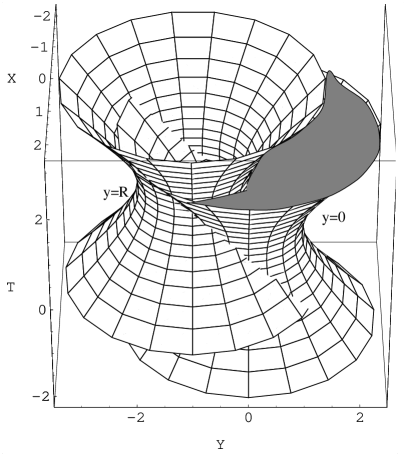
Figure 1: Illustration of the $\rho_{1}=-\rho_{2}$ solution with parameters $k=0$, and $K>0$ (note that two spatial dimensions have been suppressed) in the case where the bulk is flat space. The location of the bulk (indicated by the shaded region) is determined by the curvatures of the boundaries. While the hyperboloids are seen to intersect, they do so on the plane $Y+T=0$, a surface which can never be reached by an observer in the shaded region.

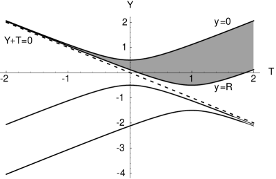
Figure 2: Two-dimensional ($\vec{X}=0$) projection of the previous figure (with $k=0$, and $K>0$). The bulk (as determined by the curvature of the domain walls) is indicated by the shaded region. Note that the bulk region satisfies the requirement that it is above the dotted line $Y+T=0$, as required for it to be within the physically accessible coordinate patch (defined by $Y+T>0$).

While the intrinsic curvature of each hyperboloid is given by $|\rho_{i}|$, the sign of $\rho_{i}$ determines on which side of the hyperboloid the bulk extends. The bulk lies outside (inside) the hyperboloid if $\rho_{i}<0$ ($>0$). As an example, figure 1 shows the solution with $\rho_{1}=-\rho_{2}$ and parameters $k=0$ and $K>0$, (where we have suppressed two spatial dimensions). In accordance with the above discussion, the portion of space-time consistent with $\rho_{1}>0$ and $\rho_{2}<0$ is indicated by the shaded region. From (38) we see that the two hyperboloids intersect in the cylinder $Y+T=0$, $\vec{X}^{2}=1/\rho_{1}^{2}$. Since $Y+T=0$ is a null plane and given our initial coordinate patch, it is easy to show that no observer in the shaded region can ever reach this intersection. Due to the symmetry in the $\vec{X}$ directions, it is sufficient for our purposes to focus on the two-dimensional projection onto the $\vec{X}=0$ plane (shown in fig. 2 for the above example). An important point to notice is that the hyperbolas are separated by a null vector (as mentioned in the second point above), and therefore share a common asymptote.

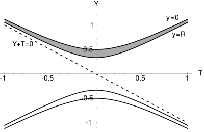
Figure 3: Illustration of the solution with $-\rho_{2}>\rho_{1}>0$ and $K=0$ projected onto the $\vec{X}=0$ plane (corresponding to $B=0$). Once again, the bulk corresponds to the shaded region. While the lower half of the figure could also yield a consistent bulk region, it lies outside the range of our original coordinates.

We can also consider examples where the curvatures of the hyperboloids are not equal, once again focusing on the subspace $\vec{X}=0$. For simplicity, let us set $k=0$. The case $K=0$ with $-\rho_{2}>\rho_{1}>0$ is shown in figure 3, with the bulk indicated by the shaded region. Note that the branes never intersect for $K=0$. Furthermore, it is crucial that $-\rho_{2}>\rho_{1}$ in order to obtain a bulk region that is simultaneously inside one brane and outside the other, which is equivalent to the condition stated below equation (33).

For the case $K\neq 0$, we see from (38) that the hyperboloids now do intersect in the paraboloid

$$Y+T=B\equiv\frac{\rho_{2}^{-2}-\rho_{1}^{-2}}{(\rho_{1}/\rho_{2}^{2})(K+k)-k/\rho_{1}}$$

$$Y-T=-\frac{1}{B}\vec{X}^{2}+\frac{1}{B\rho_{1}^{2}}-\frac{k}{\rho_{1}}.$$ (40)

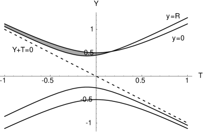
Figure 4: Illustration of the solution with $-\rho_{2}>\rho_{1}>0$ and $K<0$ (and thus, $B>0$).

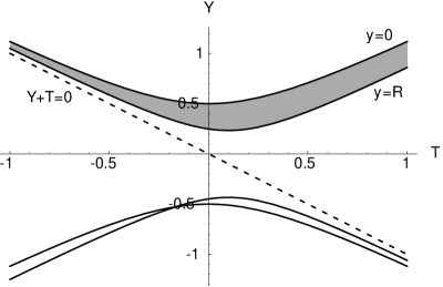
Figure 5: Illustration of the solution with $-\rho_{2}>\rho_{1}>0$ and $K>0$ ($B<0$).

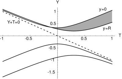
Figure 6: Illustration of the solution with $0<-\rho_{2}<\rho_{1}$ and $K>0$ ($B>0$).

Note that, as above, the intersection lies in a null plane. Furthermore, since our coordinates are restricted to $Y+T>0$, the intersection lies within our coordinate patch only if $B>0$. The solution for $-\rho_{2}>\rho_{1}>0$ with $K<0$ and $K>0$ are illustrated in figures 4 and 5, respectively. These two figures are related by reflections about the $T$ and $Y$ axes, but they should be viewed as distinct solutions in our analysis due to the constraint $Y+T>0$. In particular, the intersection lies in the physically accessible region in figure 4, where $B>0$, but not in figure 5, where $B<0$. Finally, if $\rho_{1}>-\rho_{2}$, the only choice consistent with there being a bulk between the two branes in the region $Y+T>0$ is $K>0$, in which case there is also an intersection in our coordinate patch, as illustrated in figure 6. (For the case $K<0$, the signs of the brane tensions do not allow for a bulk region between them in the region $Y+T>0$.)

We have shown that a broad class of configurations can be embedded in flat space, namely those consisting of null-separated de Sitter surfaces. The fact that we have only encountered cases with null separation is surprising, and leads us to question the generality of the solutions obtained in section 2. Intuitively, one would also expect cases with time-like and space-like separated hyperboloids. We shall confirm this intuition in section 5.

3.1 Dynamics of the orbifold

We next want to investigate the evolution of the orbifold as seen by an observer on the brane at $y=0$. First, let the cosmological time for this observer be denoted by $t^{(1)}$ (i.e., $t^{(1)}$ puts the induced metric at $y=0$ in the form given in eq. (32)). The range $-\infty<t^{(1)}<\infty$ is mapped to the range $-\infty<T<\infty$, with the rule that $t^{(1)}$ increases with $T$ in the region $Y+T>0$. Note that requiring the time coordinate to be cosmological time at $y=0$ does not uniquely fix the surfaces of constant time away from the brane. In this sense, the distance between the branes is not a coordinate-independent notion. However, a natural prescription is the following. First, choose coordinate such that the metric has the form (2). Then recall that we have seen that that neither the function $p(x)$ nor $k$ in the solution encode physical information. Thus it is natural to take the case $p={\rm const}$ and $k=0$. One then denotes the separation as the distance in the $y$-direction with fixed $t$ and $\vec{x}$ in this metric.

As seen in figures 2-6, we have five physically distinct solutions to consider, which we classify into three cases.

• $-\rho_{2}>\rho_{1}$:

  • $K=0$: This solution is shown in figure 3. As mentioned at the end of section 2, it has a static orbifold due to the choice $p=const$. The physical length of the orbifold is given by the $\lambda\rightarrow 0$ limit of equation (33), namely

    $$R_{static}\rightarrow\frac{1}{\rho_{1}}+\frac{1}{\rho_{2}},$$ (41)

    and agrees with the expression found in Ref. [7]. Finally, the curves of constant $t^{(1)}$ are straight lines trough the origin.

  • $K<0$: This solution corresponds to the shaded region in fig. 4. If we denote the physical distance between the branes by $R_{phys}$ in this case, one finds that $R_{phys}\rightarrow R_{static}^{-}$ as $t^{(1)}\rightarrow-\infty$. As $t^{(1)}$ increases, the distance between the domain walls decreases until it reaches zero size (corresponding to the point where the hyperboloids intersect). Hence, if we define the onset of inflation to occur at at some $t^{(1)}_{0}$, where $-\infty<t^{(1)}_{0}<t^{(1)}_{collapse}$, this solution describes an initial condition where the branes are within $R_{static}$ apart, and subsequently move toward each other.

  • $K>0$: In this case (shown in fig. 5), $R_{phys}\rightarrow R_{static}^{+}$ as $t^{(1)}\rightarrow-\infty$. Subsequently, $R_{phys}$ increases forever.

  Hence, for the case $-\rho_{2}>\rho_{1}$, the orbifold remains static if the initial distance is $R_{static}$, collapses if it is less than $R_{static}$, and greater if it is larger than $R_{static}$. This conclusion agrees with the analysis of Ref. [8].

• $-\rho_{2}<\rho_{1}$: This solution was not discussed in Ref. [8]. From figure 6, we see that it describes an orbifold starting from zero size and expanding to infinity. Hence, in this case, any initial distance leads to expansion.

• $-\rho_{2}=\rho_{1}$: By comparing figures 2 and 6, we see that the evolution is the same as in the case $-\rho_{2}<\rho_{1}$.

As mentioned earlier, different choices of $p$ correspond to different observers in the sense that they are associated with diffeomorphisms which leave the bulk metric in the form (2) and the induced metric at $y=0$ in the form (32). The notion of the separation of the branes is coordinate dependent. To see this explicitly suppose, for instance, we allow for a generic choice of $p$. It turns out that an observer at $y=0$ will then see, on top of the average behavior of the extra dimension, an oscillatory component. For instance, in the case $-\rho_{2}<\rho_{1}$, the orbifold would oscillate as it expands. Note that, given the restrictions imposed by equations (13) and (14), the function $p$ must be chosen such that its oscillations will not lead to $R_{phys}$ reaching zero size where it would not in the case $p=const$.

Nonetheless, there is also an observer-independent statement one can make about the various solutions described above. We noted that, in general, the branes intersect in a paraboloid (3). This intersection lies in the coordinate patch $Y+T>0$ if $B>0$. Furthermore, it lies a finite distance in the future of any observer in the bulk (corresponding to an orbifold collapsing to a final singularity) if $-\rho_{2}>\rho_{1}>0$, or in the past (corresponding to an orbifold expanding from an initial singularity) if $\rho_{1}>-\rho_{2}>0$. Finally, let us note that the surface of intersection is formally a singular surface and, thus, our solution breaks down in its neighborhood. A full treatment of brane collisions would require including effects due to the finite thickness of the branes (usually of string size).

3.2 Causal properties

Let us now consider the causal properties of the solution. More precisely, we want to see if the walls are causally-connected during the inflationary period, and whether two-way or one-way communication between the walls is possible.

In the cases where the orbifold collapses or remains static (i.e. $K\leq 0$), two-way communication is possible for all times, as expected.

The remaining solutions involve expanding orbifolds. Since the extra dimension is in fact inflating, one would expect that a signal sent from one brane could never reach the other. However, we must keep in mind that the length of the orbifold is computed along a space-like path, while gravitons propagate along null geodesics. Consequently, the causal properties are not as trivial as one would have guessed. The analysis yields qualitatively the same result for all solutions which describe expanding orbifolds, so, without loss of generality, we can focus on the case $\rho_{1}=-\rho_{2}$ for concreteness. Suppose observer 2 at $y=R$ sends signals to observer 1 at $y=0$. The two dotted lines in figure 7 correspond to two such signals. We see that the first signal reaches $y=0$ in finite affine parameter while the other does not. Hence, from the point of view of observer 2, there exists some time on his clock where his signals stop reaching the $y=0$ brane. We shall say that a causal boundary has appeared for observer 2. Now, consider signals sent from $y=0$ towards $y=R$. It is clear from figure 7 that such signals always reach $y=R$ in finite affine parameter. However, if $t^{(1)}$ is physical time for observer 1, then after a while observer 1 sees his signals taking infinite time $t^{(1)}$ to reach $y=R$. From the point of view of observer 1, we shall say that there is a horizon somewhere in the bulk. Note that this is not a genuine horizon in the five-dimensional space-time, but corresponds to a surface with the following property: once a signal sent by observer 1 has passed through the horizon, it cannot return to observer 1. Note that causality implies that the appearance of a horizon requires the appearance of a causal boundary, and vice versa. To see this, suppose the contrary is true; that is, suppose that there is a horizon for observer 1 but no causal boundary for observer 2. If observer 1 sends a graviton towards $y=R$, because of the horizon he will see his graviton frozen somewhere in the bulk. On the other hand, observer 2 will receive this signal within finite time on his clock. If observer 2 replies to the signal, his reply will be received at $y=0$ in finite time on observer 1’s clock (because we have assumed that there were no causal boundary). From the point of view of observer 1, he received a reply from observer 2 before his initial signal made it to $y=R$, an obvious violation of causality. It is easily seen that the horizon and causal boundary describe the same surface in the bulk, namely the future light cone asymptotic to the $y=0$ hyperboloid. That is, once observer 2 is within this surface, his signals will not reach $y=0$ in finite affine parameter.

To summarize our conclusions for expanding extra dimensions, our solution predicts that two-way communication is only possible for a finite amount of time. Afterwards, only the brane with positive tension can send signals to (and, hence, have influence on) the negative-tension brane.

4 Geometrical analysis of $\lambda<0$ solution

In this section, we generalize the analysis of the previous section to the case of negative bulk cosmological constant. As there, we will find that all the solutions presented in section 2 correspond to the same bulk space-time. In this case it is AdS₅. We can therefore think of our solution as a class of possible ways to embed two dS₄ surfaces in AdS₅. As in the case of flat space discussed in the previous section, we shall find evidence that our solution does not describe the full spectrum of such embeddings.

Recall that the general bulk solution has the form (12)

$$ds^{2}=\frac{1}{(f+g)^{2}}\left(\frac{4}{\lambda}f^{\prime}g^{\prime}(-d\tau^{2}+dy^{2})+d\vec{x}^{2}\right),$$ (42)

With the line element in this form, it is not clear that, in fact, for $\lambda<0$, in all cases the bulk geometry is that of AdS₅. However, upon the coordinate transformation

$$z+t=\frac{2}{\sqrt{-\lambda}}f$$

$$z-t=\frac{2}{\sqrt{-\lambda}}g,$$ (43)

we have

$$ds^{2}=\frac{1}{(-\lambda)z^{2}}(-dt^{2}+d\vec{x}^{2}+dz^{2}),$$ (44)

which is a more familiar form for the line element of AdS₅. We see that the general functions $f$ and $g$ simply represented different choices of conformal coordinates $\tau$ and $y$ in the AdS₅ space.

As is well known, this coordinate system does not cover the whole of AdS space. More generally one can describe AdS as a hyperboloid [16]

$$-X^{2}\equiv T_{1}^{2}+T_{2}^{2}-Y^{2}-\vec{X}^{2}=\frac{1}{-\lambda}$$ (45)

embedded in a flat six-dimensional space $X=(T_{1},T_{2},Y,\vec{X})$ with line element

$$ds^{2}=dX\cdot dX\equiv-dT_{1}^{2}-dT_{2}^{2}+dY^{2}+d\vec{X}^{2}.$$ (46)

We should note here that the space described contains closed time-like curves. The full AdS space is really the universal covering space. This will not enter our analysis here, since in all our solutions the domain walls will lie in the same sheet of the universal cover. In terms of the coordinates in (44) the embedding is given by

$$T_{1}+Y=\frac{1}{(-\lambda)z}$$

$$T_{1}-Y=\frac{\vec{x}^{2}-t^{2}+z^{2}}{z}$$

$$T_{2}=\frac{t}{\sqrt{-\lambda}z}$$

$$\vec{X}=\frac{\vec{x}}{\sqrt{-\lambda}z}.$$ (47)

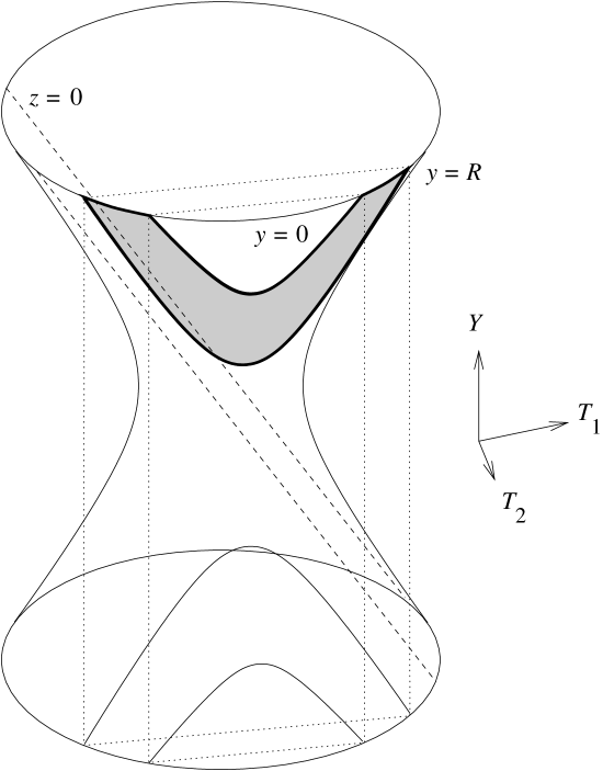
Figure 8: Sketch of the solution with $\lambda<0$, $-\rho_{2}>\rho_{1}>0$, and $K=0$. The resulting space-time (indicated by the shaded region) is obtained by intersecting the AdS₅ hyperboloid with two planes of constant $T_{2}$.

Note that since $z=(f+g)/\sqrt{-\lambda}>0$, our original coordinates are mapped to the range $T_{1}+Y>0$. (The boundary of this region, $z=0$, is shown in figure 8.)

Let us now turn to the description of the domain walls. Recall that in our original coordinates the walls were fixed at $y=0$ and $y=R$, or equivalently $x^{+}=x^{-}$ and $x^{+}=x^{-}+2R$. After the conformal transformation (43) the walls will now be moving in the $z$ direction. Explicitly, from the relations (21), the equations of the walls in terms of $z$ and $t$ are the linear relations

$$\displaystyle t-z=\gamma_{1}^{2}(t+z)+\frac{2k_{1}}{\sqrt{-\lambda}} \qquad\textrm{for $y=0$};$$ (48)

$$\displaystyle t-z=\gamma_{2}^{2}(t+z)+\frac{2k_{2}}{\sqrt{-\lambda}} \qquad\textrm{for $y=R$}.$$

It is easy to see that in these coordinates, the domain walls move in the $z$ direction with constant velocity $H_{i}/|\rho_{i}|$.

Finally we can transform these equations into the flat six-dimensional embedding space. One finds that the walls correspond to planes

$$\displaystyle\pm T_{2}+k_{1}\left(\frac{\rho_{1}}{H_{1}}\mp 1\right)(T_{1}+Y)=\frac{\rho_{1}}{\sqrt{-\lambda}H_{1}} \qquad\textrm{for $y=0$};$$ (49)

$$\displaystyle\pm T_{2}+k_{2}\left(\frac{|\rho_{2}|}{H_{2}}\mp 1\right)(T_{1}+Y)=\frac{|\rho_{2}|}{\sqrt{-\lambda}H_{2}} \qquad\textrm{for $y=R$}.$$

The choice of signs correspond to the choice of sign in the expressions (22) for $\gamma_{1}$ and $\gamma_{2}$.

Note that both these equations have the form, for $i=1,2$,

$$n_{i}\cdot X=c_{i}$$ (50)

where $n_{i}$ is a time-like unit vector and $c_{i}>1/\sqrt{-\lambda}$. Intersecting with the AdS₅ hyperboloid (45), one finds that the domain walls are dS₄ submanifolds of the embedding space of curvature

$$\left(c_{i}^{2}+\frac{1}{\lambda^{2}}\right)^{-1/2}=H_{i},$$ (51)

where we have substituted the particular form of $c_{i}$ from equation (49). (This can be seen explicitly by using the $SO(4,2)$ symmetry of the embedding flat space to put $\vec{n}=(1,0,\dots,0)$ and substituting in eqn. (45)). Thus we see again how the domain walls are indeed dS₄ surfaces in the AdS₅ space with curvatures $H_{i}$.

To get a sense of the global structure of the solution consider the case where $k_{1}=k_{2}=0$ and choose the upper signs in the solution (49). The planes are then simply given by $T_{2}=|\rho_{i}|/(H_{i}\sqrt{-\lambda})$. The intersection is sketched in figure 8. Note that in this case, the branes never intersect. The figure allows to understand how the curves describing the domain walls would turn into the hyperbolas shown in figure 3 if we let $\lambda\to 0$. Intuitively, we can generate the solutions described above by taking the hyperbolas of the previous section and “pasting” them on the hyperboloid as shown in figure 8. We can use this intuition to realize that the various parameters (e.g., $k$, $p$, etc.) describing the solution play a similar role as in the case $\lambda=0$. However, we should also note that, in general, there is a second class of solutions where we make the opposite choice of signs for the two walls in (49). (Actually this choice is not possible for the specific case $k_{1}=k_{2}=0$.) Now the planes are on “opposite sides” of the AdS hyperboloid. This has no natural $\lambda\to 0$ limit. It corresponds to the result of section 3 that we were forced to choose a correlated signs in $\gamma_{i}$ to get the flat-space solution.

As a second example, we can briefly mention that the domain walls in the Randall–Sundrum scenario (taking the $|\rho_{i}|\to\sqrt{-\lambda}$ limit in eqns. (49)) are described by the null planes

$$\displaystyle T_{1}+Y=\frac{1}{k_{1}\sqrt{-\lambda}} \quad\textrm{for $y=0$},$$ (52)

$$\displaystyle T_{1}+Y=\frac{1}{k_{2}\sqrt{-\lambda}} \quad\textrm{for $y=R$},$$

Again these branes will never intersect.

To cast the above discussion in a more general set-up, recall that in the previous section, the relative position of domain walls was characterized in flat space by their Minkowskian distance (more formally, by the distance between their asymptotic light cones). Furthermore, in general this separation was null for the solutions of section 2. Similarly here, the asymptote of each dS in the six-dimensional embedding space is a light cone, whose origin lies at

$$a_{i}=c_{i}n_{i}\qquad\textrm{for $i=1,2$}.$$ (53)

Note that, in general, the vector $a_{i}$ will not lie on the bulk AdS hyperboloid. We can now use the distance between the light cones, given by

$$D\equiv a_{1}-a_{2},$$ (54)

to characterize the relative location of the dS surfaces in a coordinate-independent way. Furthermore, it is easily seen that the quantity $D$ does reduce to the distance between hyperboloids in the limit $\lambda\rightarrow 0$, as defined in section 3. Just as in the case $\lambda=0$ where our solutions all described null separated hyperboloids, similarly, it can be easily verified from equations (49) that all our $\lambda<0$ solutions with a flat limit yield $D^{2}=0$, corresponding to null separation. The size of the separation is controlled by the parameters $k_{1}$ and $k_{2}$.

Once again, we expect that solutions with time-like and space-like separated dS surfaces are also allowed. We shall discuss these more general configurations in section 5.

Finally, we note that the dynamics of the orbifold as well as the causal properties of the solution are qualitatively the same as for the case $\lambda=0$. The nature of the intersection between the walls is controlled by $n_{i}$ and $\rho_{i}$. For general $n_{i}$, the intersection is a null paraboloid. As before there are two cases, one where the space-time has either expands from an initial singularity and one which contracts to a final singularity. For the special case where the $n_{i}$ are parallel or anti-parallel, there is no intersection and the distance between the walls is fixed. For example, in the case $-\rho_{2}>\rho_{1}>0$, we find that the orbifold remains static if the initial distance between the branes equals $R_{static}$ (see eqn. (33)) and expands (collapses) if it is larger (smaller) than $R_{static}$. Furthermore, two-way communication is only possible for a finite amount of time if the extra dimension is expanding.

5 General embedded solutions

In this section we will step back a little and reconsider the solutions given thus far. In doing so we will see that they are in fact special cases of a more general configuration of a pair of branes in bulk AdS space. Note that in this section our solutions will also no longer be confined to a particular coordinate patch of AdS space.

From the discussion of previous section, the solutions we found correspond to a pair of dS surfaces embedded in AdS space. The dS surfaces are not in general position but are null separated in the sense discussed below eqn. (54). Recall that the solutions were found by solving the bulk Einstein equation with negative cosmological constant together with the Israel matching conditions describing the discontinuity in the normal derivative of the metric at the brane.

The important point to note is that once we fix the bulk solution, in this case to be AdS, the solution of the Israel conditions for the two walls are completely independent. Each set of conditions are local equations relating the shape of the brane embedded in the bulk space to the stress energy on that brane, independent of the second brane. From the analysis of the previous two sections, it appears that for pure cosmological constant $\rho$ on the brane, the solution to the Israel conditions is that the brane describe a dS surface embedded in AdS. If this is correct, it is then clear that the general solution corresponds to a pair of dS brane embedded in AdS with arbitrary separation.

To see that this is indeed the case, we can consider the Israel conditions in a coordinate independent form and show that, when the bulk space is AdS₅, they imply that the brane is a dS₄ surface. If we let $t^{\mu}$ be the normal vector to the brane, the induced metric $g^{4}_{\mu\nu}$ is then given by

$$g_{\mu\nu}=g^{4}_{\mu\nu}+t_{\mu}t_{\nu},$$ (55)

where $g_{\mu\nu}$ is the bulk metric. As has been noted in various papers (see e.g., [11]), assuming $Z_{2}$ reflection invariance at the brane, the Israel conditions relate the extrinsic curvature $K_{\mu\nu}$ of the brane to the stress energy $T^{B}_{\mu\nu}=-6\rho g^{4}_{\mu\nu}$ on the brane. One has

$$K_{\mu\nu}=-\frac{1}{2}\left(T^{B}_{\mu\nu}-\frac{1}{3}T^{B}g^{4}_{\mu\nu}\right)=-\rho g^{4}_{\mu\nu},$$ (56)

where the extrinsic curvature is given by

$$K_{\mu\nu}=g_{\ \mu}^{4\ \rho}g_{\ \nu}^{4\ \kappa}\nabla_{\rho}t_{\kappa}.$$ (57)

Since $g^{4}_{\mu\nu}$ and $t_{\mu}$ are functions of the embedding, equation (56) is a local differential equation for the functions describing the embedding of the brane in AdS₅, completely independent of the presence of a second brane.

To show that a dS₄ surface satisfies the Israel conditions, we could evaluate (56) in a particular set of coordinates. This is essentially what was done in section 2. Alternatively, we can argue simply by symmetry that if the brane is dS the extrinsic curvature must be proportional $g^{4}_{\mu\nu}$, since this is the only symmetric tensor on the brane with the correct symmetries. The only question is then what curvature of the dS space must we choose to make the constant of proportionality exactly that in (56). To answer this we recall that there is an expression for the intrinsic curvature $R_{4}$ of $g^{4}_{\mu\nu}$ in terms of the bulk curvature $R$ and $K_{\mu\nu}$. In particular, we have the general expression

$$R^{4}_{\kappa\lambda\mu\nu}=g_{\ \kappa}^{4\ \kappa^{\prime}}g_{\ \lambda}^{4\ \lambda^{\prime}}g_{\ \mu}^{4\ \mu^{\prime}}g_{\ \nu}^{4\ \nu^{\prime}}R_{\kappa^{\prime}\lambda^{\prime}\mu^{\prime}\nu^{\prime}}+K_{\kappa\mu}K_{\lambda\nu}-K_{\kappa\nu}K_{\lambda\mu}.$$ (58)

Substituting the form of $K_{\mu\nu}$ and the bulk AdS space curvature $R_{\kappa\lambda\mu\nu}=\lambda\left(g_{\kappa\mu}g_{\lambda\nu}-g_{\kappa\nu}g_{\lambda\mu}\right)$ gives the intrinsic scalar curvature

$$R_{4}=12\left(\rho^{2}+\lambda\right).$$ (59)

We have reproduced the result we derived in section 2. The curvature of the brane dS space is such that the square of the Hubble constant (see eq. (30)) is $\rho^{2}+\lambda$.

One notes that the curvature (59) of the brane is independent of the sign of the brane tension $\rho$. What then distinguishes the $\rho>0$ case from $\rho<0$? Since the brane is a codimension-one boundary in AdS space, we can either take the bulk space-time to be the space “inside” the dS boundary or “outside” the dS boundary. Consider Figure 9, which shows the intersection of two planes with the AdS hyperboloid. Let us focus on the left-hand plane, corresponding to a single dS submanifold. By “inside” we mean that the bulk space-time includes the throat of the AdS hyperboloid. By “outside” we mean that the bulk space-time is one of the two disconnected regions which do not include the throat. For example, the solid circle in figure 9 lies ”inside” the dS boundary, while the open circle lies ”outside” it. These two regions are distinguished by the direction of the normal vector $t_{\mu}$. Furthermore they have opposite extrinsic curvature $K_{\mu\nu}$. It is then easy to show that one has the following conditions

$$\begin{array}[]{c}\textrm{if $\rho>0$ then the spacetime is ``inside'' the dS boundary}\\ \textrm{if $\rho<0$ then the spacetime is ``outside'' the dS boundary}.\end{array}$$ (60)

We can now give a geometrical description of the general embedding solution. As we argued above, since the Israel conditions are local we can choose the branes to lie on any pair of dS surfaces. As noted in the previous section, in general, these are described by the intersection of an arbitrary pair of planes with the AdS hyperboloid. This is shown in Figure 9. For generic choices of $n_{1}$ and $n_{2}$ the dS spaces will always intersect transversally. This means there are configurations for all values of the signs of $\rho_{1}$ and $\rho_{2}$. However, if $n_{1}$ and $n_{2}$ are either parallel or anti-parallel this is no longer true. In these cases the branes never intersect. As a result, if the vectors are parallel, one only has a solution with a bulk space-time bounded by a pair of branes if $-\rho_{1}>\rho_{2}>0$ or $-\rho_{2}>\rho_{1}>0$. In the case where they are anti-parallel one requires $\rho_{1}>0$ and $\rho_{2}>0$.

The analysis of sections 3 and 4 allowed us to realize that the solutions obtained in section 2 all described de Sitter surfaces separated by a null vector. The above discussion has shown that time-like as well as space-like separation vectors are also allowed. Furthermore, given that two time-like vectors of equal magnitude are related by a boost, the degrees of freedom describing the general solution are: the brane tensions, the magnitude of the separation vector, and whether it is null, space-like, or time-like. In addition, we note that, except for the special case where the planes describing the dS branes are parallel or anti-parallel, there are in general no conditions on the signs of $\rho_{1}$ and $\rho_{2}$ for a solution to exist. The condition we found in section 2 is an artifact of using a particular coordinate system.

The use of a specific coordinate system to analyze the null-separated solutions was useful to describe the dynamics of the extra dimension as viewed by an observer living on either brane (sec. 3.1) as well as the appearance of horizons in the bulk (sec. 3.2). However, we noted that these questions could also be addressed purely geometrically. The same is true for the general embeddings described here. Of course, if one wished, it is possible to describe the general solutions using some global coordinate system adapted to one of the branes. As mentioned in section 2, one way to proceed would be to start with the same ansatz for the metric as equation (2) but allow for a more general location of the second brane.

We end this section by noting that although discussed in the context of negative bulk cosmological constant $\lambda$ and dS branes ($\rho_{i}$ satisfying $\rho_{i}^{2}+\lambda>0$), the derivation of the embedding conditions is completely general. The construction naturally goes over to cases of positive or zero $\lambda$ and arbitrary $\rho_{i}$. For instance, in bulk dS or flat space the intrinsic brane curvature (59) is always positive and we are considering embedded dS branes. In AdS space, the intrinsic curvature can also be zero (the Randall–Sundrum case) or negative. In the latter case we are embedding AdS branes in the AdS bulk. Geometrically these arise from intersecting with planes where $n$ is null (for flat branes) or space-like (for AdS branes).

6 Discussion

All the solutions presented in this work were obtained by assuming (albeit implicitly) that the bulk was AdS. It was then found that a domain wall of uniform energy density can be embedded in this background provided it follows a de Sitter trajectory, and we described the most general configuration with two such trajectories in AdS. Rather than fixing the bulk geometry for all times, a more general approach is to treat the problem as an initial-value problem. Let us assume that the only stress-energy in the problem is a negative cosmological constant $\lambda$ in the bulk and brane tensions $\rho_{i}$ such that $|\rho_{i}|>\sqrt{-\lambda}$. Suppose we choose some space-like hypersurface on which we specify the initial spatial bulk metric and the boundary branes. In general, one could imagine complicated initial conditions, but a natural configuration to consider is one with a space-like slice of anti-de Sitter spatial bulk metric and two (spatially) flat surfaces with arbitrary separation, velocity, and orientation. If one were to solve for the time evolution of this system, one would generically find that the bulk does not remain AdS but that a non-vanishing Weyl tensor is generated. This would mean that our solutions correspond to initial conditions which are tuned so that the bulk remains AdS. Coming back to the general problem, it is not clear whether all bulk evolutions would yield homogeneous and isotropic cosmologies on the branes. It would be essential to know what subclass of initial conditions would be consistent with the usual assumptions of cosmology.

A related issue has to do with the stability of the solutions. Suppose our tuned initial conditions are perturbed, then one should investigate whether the path is only slightly or greatly disturbed by the variation. The brane motion could be perturbed either by moving the brane as a whole away from its initial trajectory without altering its energy density, by moving a region of the brane off the trajectory while keeping the energy density constant, or by perturbing the energy density in a spatially homogeneous or inhomogeneous way. In the first case, we know of at least one example of instability, namely solutions with static orbifolds in the case $\rho_{1}\neq-\rho_{2}$. Indeed, we saw in section 3 that the branes will eventually collide if brought infinitesimally closer than the static distance, or end up infinitely far apart if pulled away from each other. Note that, even though the path is unstable, the cosmological evolution remains de Sitter and the bulk is still AdS. Nevertheless, more general homogeneous perturbations may drive the bulk away from AdS and, thus, drive the cosmological evolution on each brane away from dS. As for inhomogeneous energy density perturbations, it was argued in Ref. [17] that any spatial inhomogeneities on the brane stress-energy will modify the AdS bulk through gravitational radiation. Cosmological energy density perturbations in brane-worlds have recently been investigated in Refs. [19, 20, 21, 22].

To conclude, let us briefly point out that our solutions can be straightforwardly generalized to any type of energy density on the brane (e.g., radiation, matter). Fixing the bulk metric to be AdS for simplicity, one can use the Israel junction condition at the location of the brane to solve for its motion in the bulk [11, 18], which in turn determines its cosmological evolution. If we want to embed two domain walls, each one should be allowed to travel along any trajectory consistent with its energy density.

Acknowledgments
We would like to thank Burt Ovrut, Alexander Polyakov, Andy Strominger, and Herman Verlinde for helpful discussions. J.K. is supported by the Natural Sciences and Engineering Research Council of Canada. P.J.S. is supported in part by US Department of Energy grant DE-FG02-91ER40671. D.W. would like to thank The Rockefeller University and The University of Chicago for hospitality during the completion of this work.

Figure 7: Same case as that of figure 2 except that the dotted lines now represent gravitons sent from $y=R$ towards $y=0$. This shows that after a while, signals sent from $y=R$ do not reach $y=0$ in finite affine parameter.

Figure 9: General dS₄ branes in AdS₅ space formed by the intersection of planes with the AdS hyperboloid. Consider the brane formed by the left-hand plane. The sign of its tension, $\rho$, determines where the bulk lies. If $\rho<0$, the bulk includes the throat region, so that the solid circle lies in the bulk. If $\rho>0$, the bulk excludes the throat and, for example, the open circle lies in the bulk.

References

- [1] P. Hořava and E. Witten, Nucl. Phys. B460, 506 (1996); B475, 94 (1996).
- [2] A. Lukas, B.A. Ovrut, K.S. Stelle and D. Waldram, Phys. Rev. D 59, 086001 (1999).
- [3] L. Randall and R. Sundrum, Phys. Rev. Lett. 83, 3370 (1999).
- [4] N. Kaloper, Phys. Rev. D 60, 123506 (1999).
- [5] T. Nihei, Phys. Lett. B 465, 81 (1999).
- [6] P. Kanti, I.I. Kogan, K.A. Olive and M. Pospelov, Phys. Lett. B 468, 31 (1999).
- [7] A. Lukas, B.A. Ovrut and D. Waldram, Phys. Rev. D 61, 023506 (2000).
- [8] H.B. Kim and H.D. Kim, Phys. Rev. D 61, 064003 (2000).
- [9] P. Binétruy, C. Deffayet, U. Ellwanger and D. Langlois, hep-th/9910219.
- [10] W. Israel, Nuovo Cimento 44B, 1 (1966), erratum: 48B, 463 (1967).
- [11] H.A. Chamblin and H.S. Reall, Nucl. Phys. B562, 133 (1999).
- [12] D. Ida, gr-qc/9912002.
- [13] A.H. Taub, Ann. Math. 53, 472 (1951).
- [14] J. Ipser and P. Sikivie, Phys. Rev. D30, 712 (1984).
- [15] E. Kasner, Trans. Am. Math. Soc. 27, 155 (1925).
- [16] S.W. Hawking and G.F.R. Ellis, The Large Scale Structure of Space-Time (Cambridge University Press, 1973).
- [17] T. Shiromizu, K. Maeda and M. Sasaki, gr-qc/9910076.
- [18] P. Kraus, hep-th/9910149, JHEP 9912 (1999) 011.
- [19] S. Mukohyama, hep-th/0004067.
- [20] H. Kodama, A. Ishibashi and O. Seto, hep-th/0004160.
- [21] D. Langlois, hep-th/0005025.
- [22] C. van de Bruck, M. Dorca, R.H. Branderberger and A. Lukas, hep-th/0005032.